
Machine Learning for Determining Interactions between Air Pollutants and Environmental Parameters in Three Cities of Iran


 ,
,  ,
,
Abstract
:1. Introduction
2. Materials and Methods
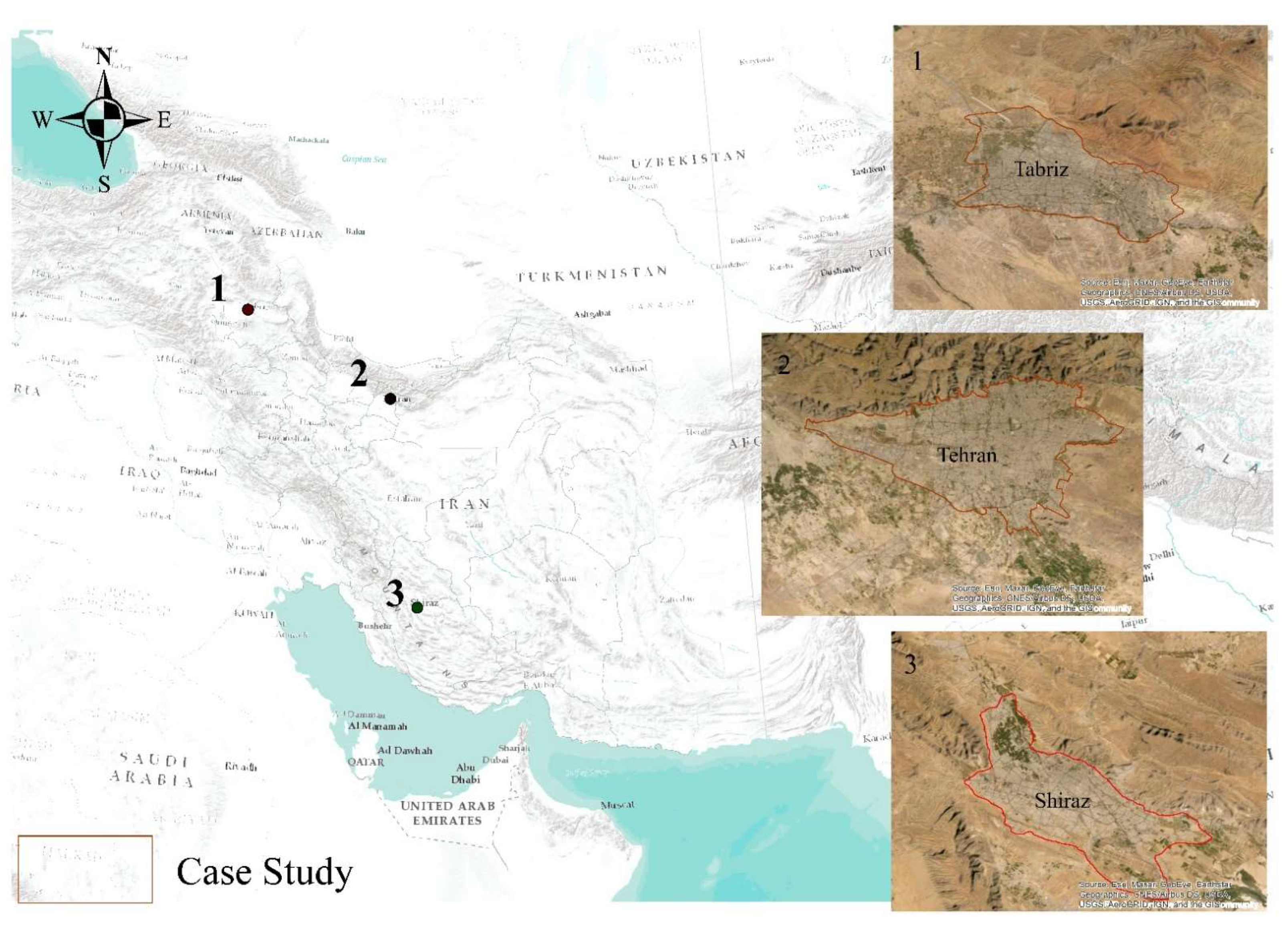
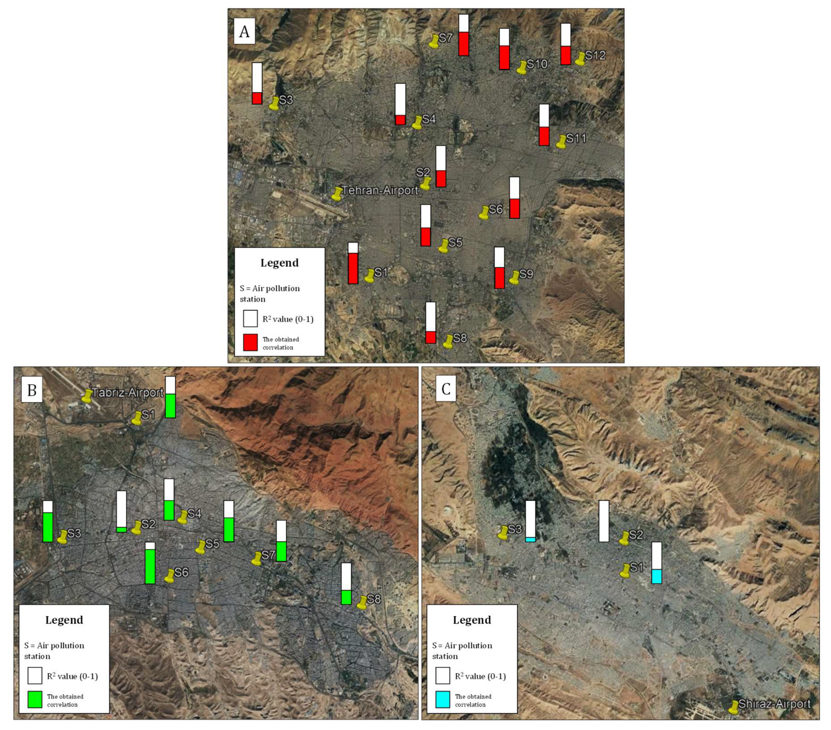
2.1. Case Study
2.2. Data
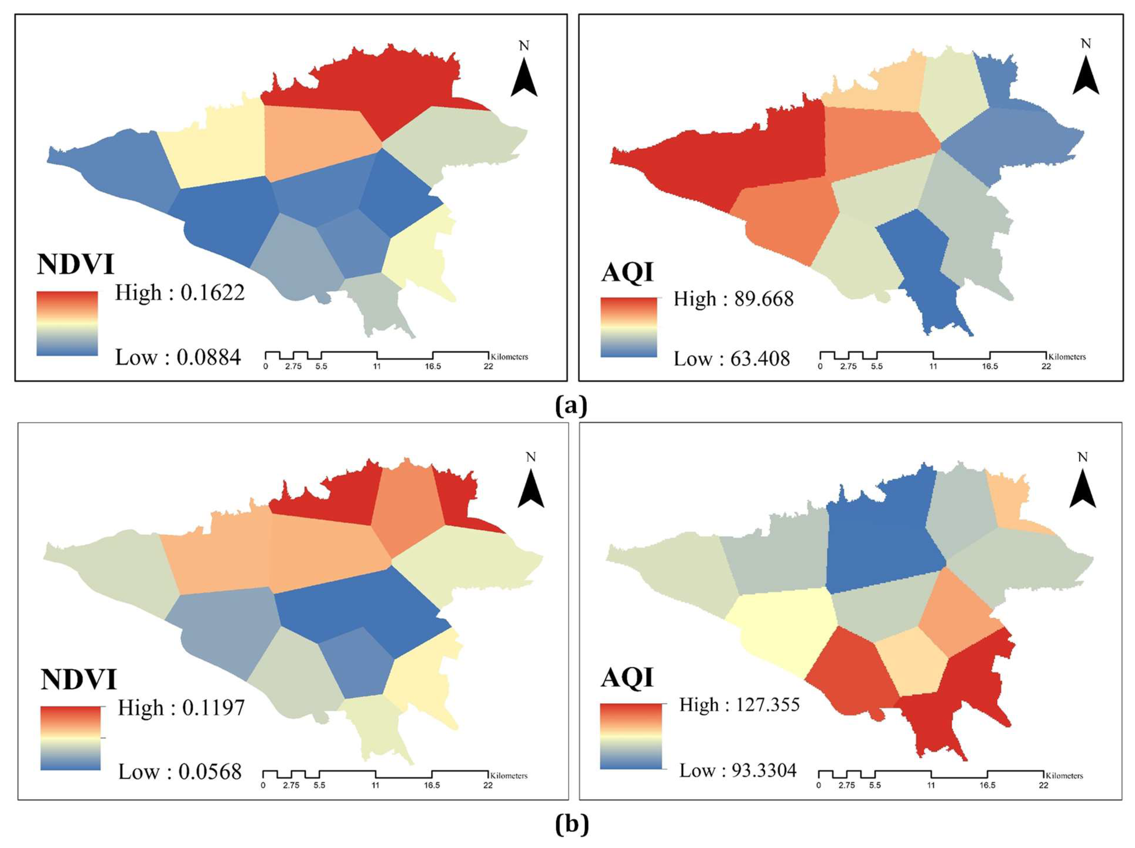
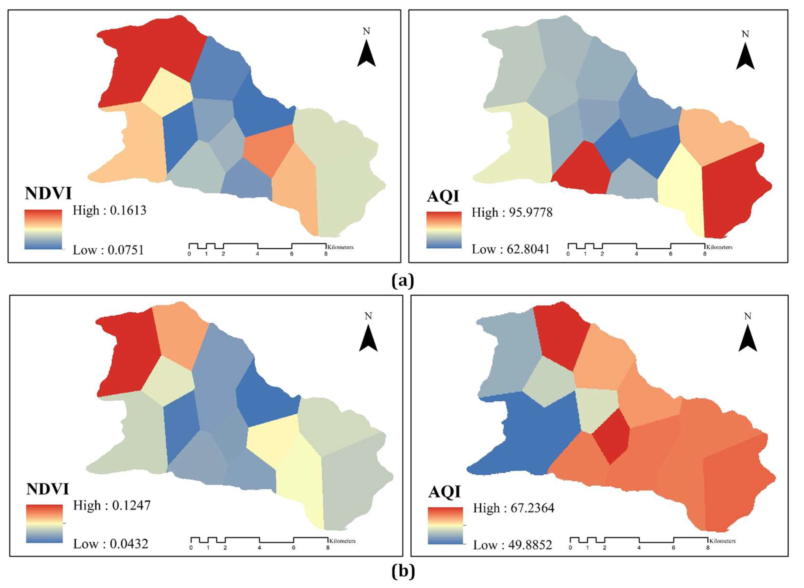
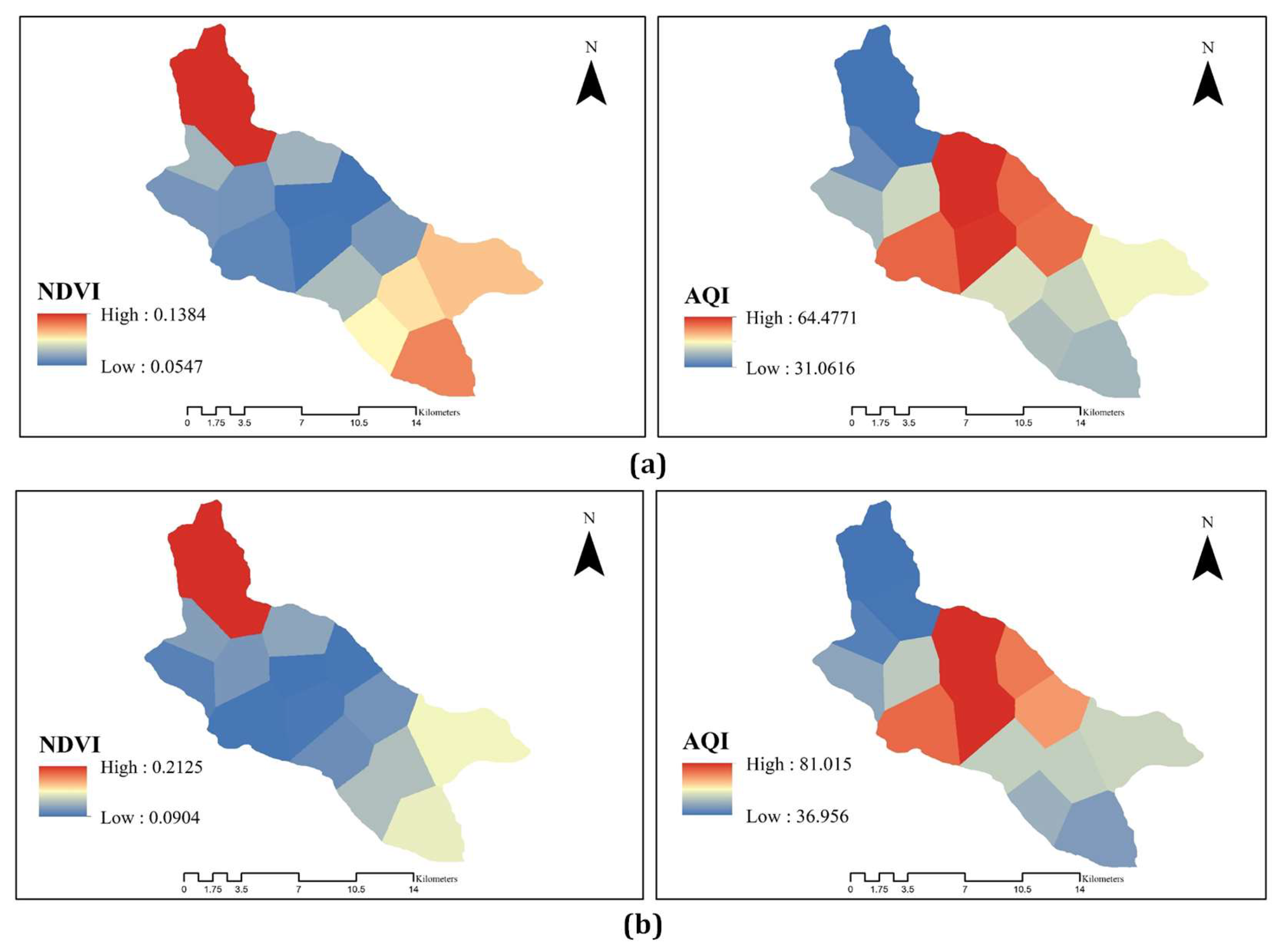
2.3. Mapping
2.4. Statistical Analyzing
2.5. Modeling
2.5.1. Hyperparameters Optimization
2.5.2. Preprocessing Dataset
2.5.3. Xgboost Training and Hyper-Parameter Optimization
2.5.4. Evaluation Metrics
3. Results and Discussion
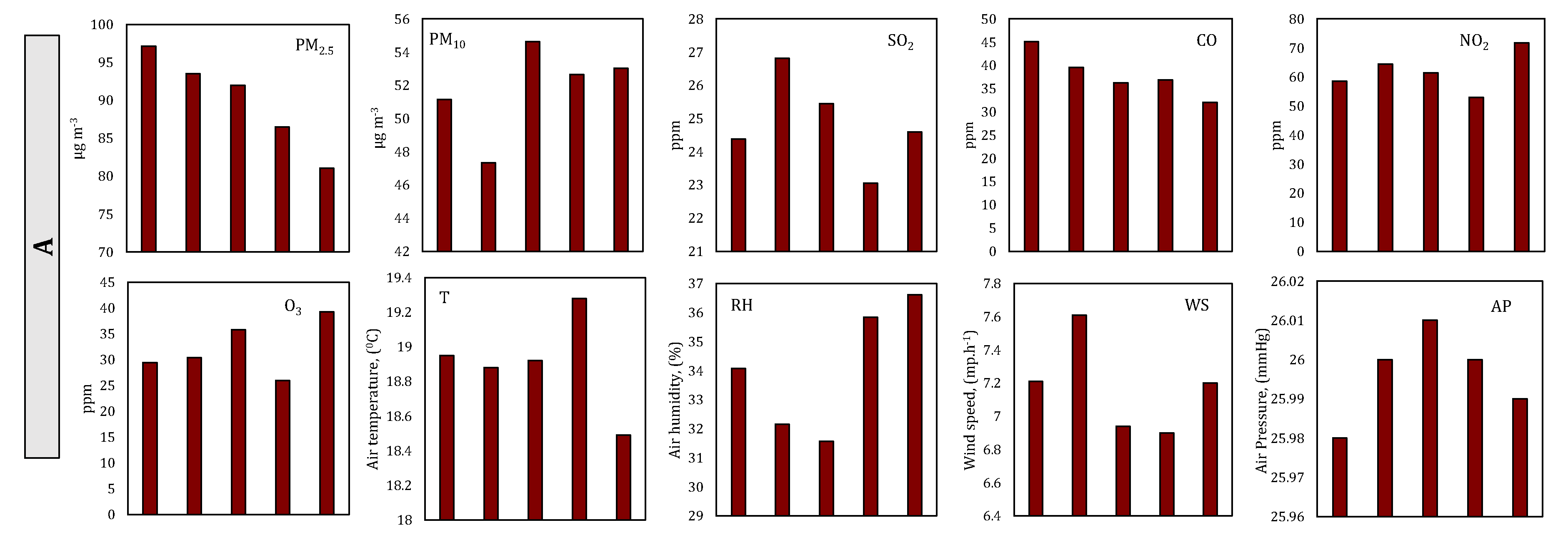
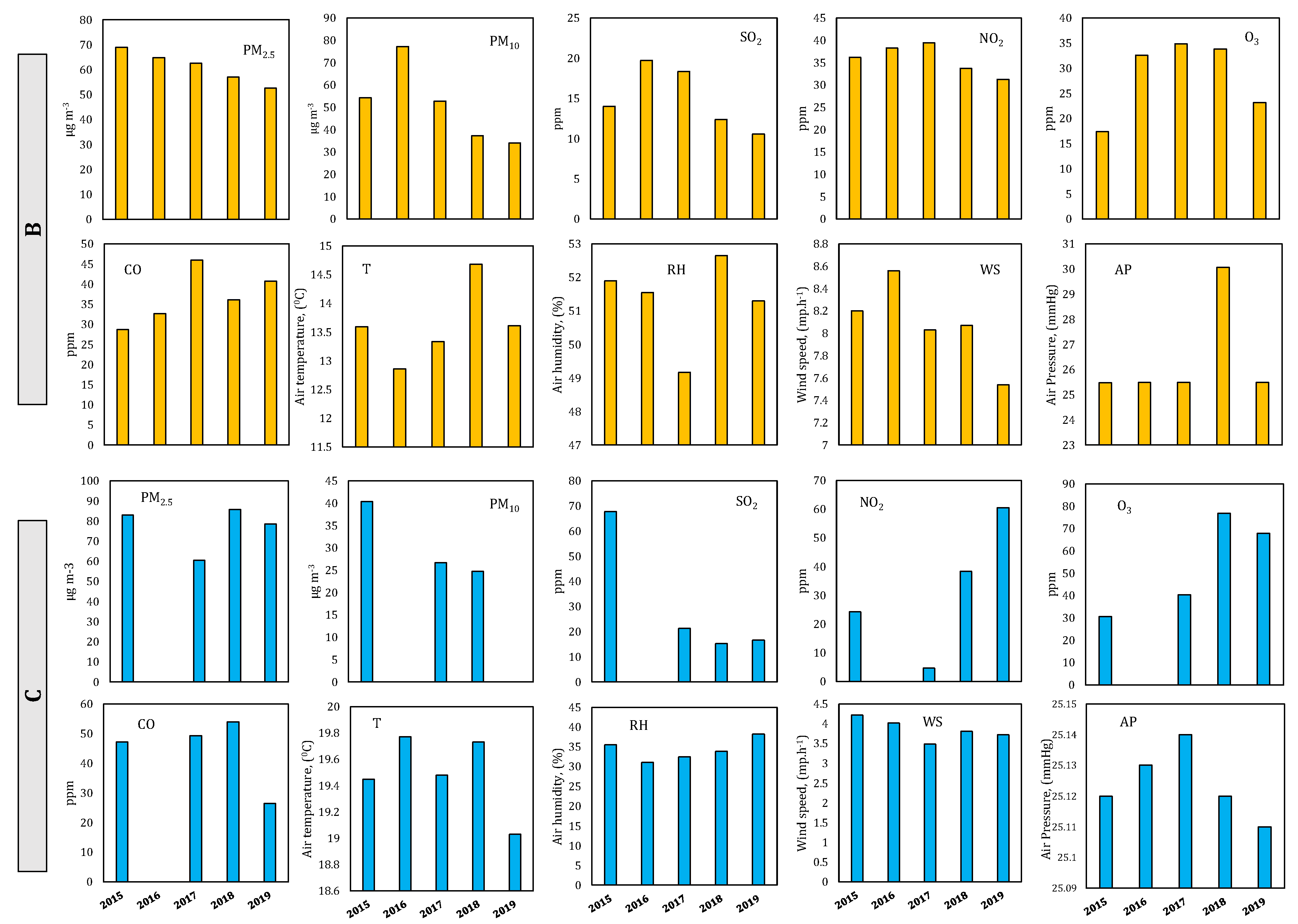
3.1. Changes of Pollutants Emission
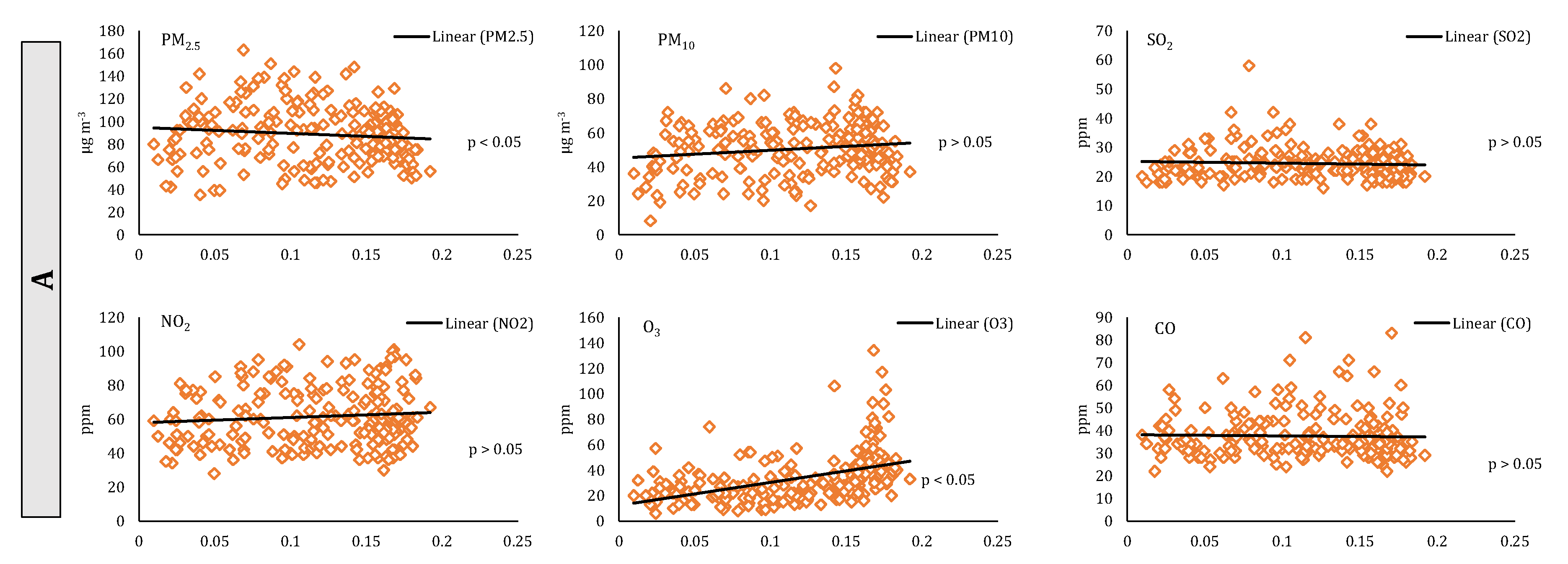
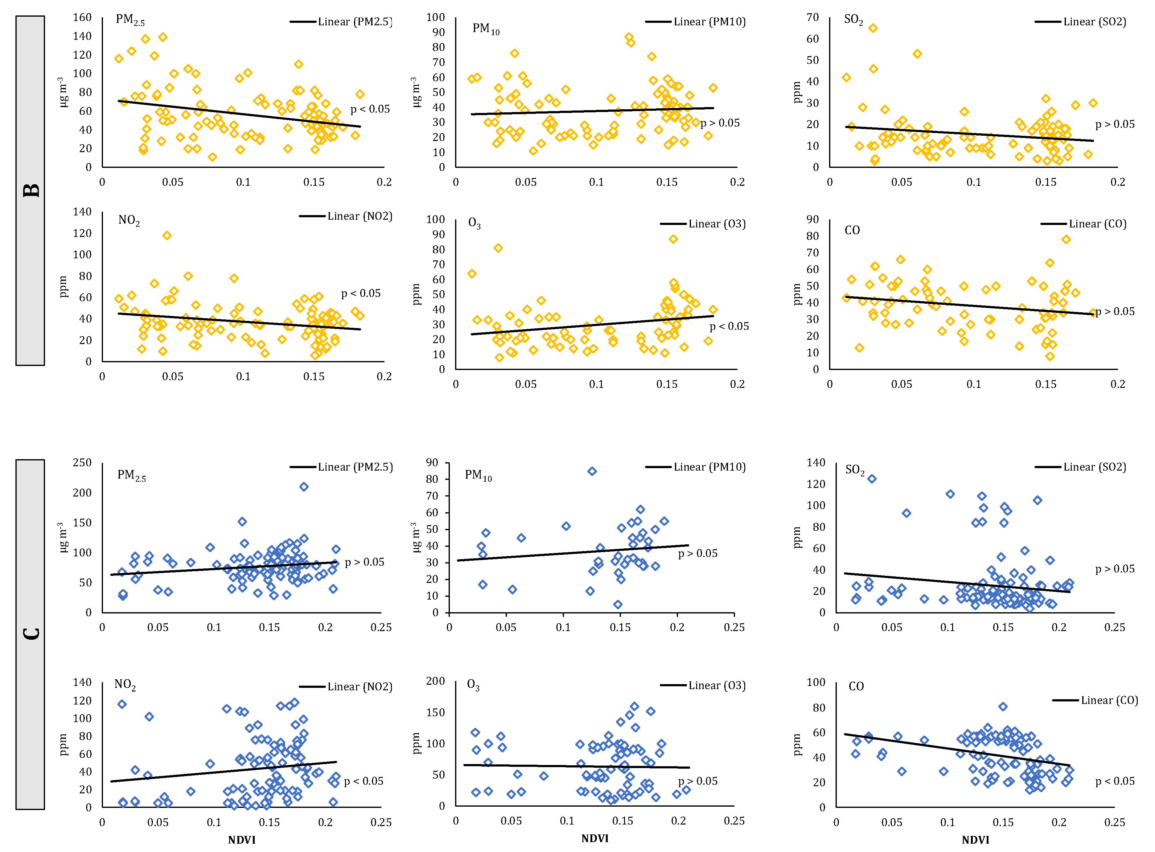
3.2. Interactions between Air Pollutants and Vegetation
3.3. Interactions between Air Pollutants and Meteorological Factors
3.4. Model Evaluation
- This survey did not consider second- and third-order interactions between parameters. Researchers should, therefore, address these interactions in the modeling process;
- It is suggested that in machine learning-based investigations, correlations across weather stations and nearby air quality stations should be explored to improve prediction accuracy [113]. In addition, it is necessary to develop dynamic and integrated air quality models employing hybrid machine learning algorithms [108];
- Modeling the emission from sources, chemical reactions of pollutants, and urban activities is required to improve forecasting accuracy [114], which was not considered in the present investigation. Eventually, clean air may only be restored whenever governments shift their approach toward sustainable environmental strategies [115].
4. Conclusions
Author Contributions
Funding
Institutional Review Board Statement
Informed Consent Statement
Data Availability Statement
Acknowledgments
Conflicts of Interest
Appendix A

| Feature No. | Feature Description | Type |
|---|---|---|
| 1 | Relative Humidity | Numerical |
| 2 | Air Pressure | Numerical |
| 3 | Temperature | Numerical |
| 4 | NDVI | Numerical |
| 5 | Wind Speed | Numerical |
| PM2.5 | PM10 | ||||
|---|---|---|---|---|---|
| Parameter | Value | Description | Parameter | Value | Description |
| Learning rate | 0.02 | Shrink the weights on each step | Learning rate | 0.0095 | Shrink the weights on each step |
| n_estimators | 350 | Number of trees to fit | n_estimators | 500 | Number of trees to fit |
| Reg_lambda | 0.25 | L2 regularization term on weights | Reg_lambda | 0 | L2 regularization term on weights |
| Booster | gbtree | Select the model for each iteration | Booster | gbtree | Select the model for each iteration |
| min_chid_weigth | 1 | Minimum sum of weights | min_chid_weigth | 5 | Minimum sum of weights |
| max_depth | 6 | Maximum depth of a tree | max_depth | 4 | Maximum depth of a tree |
| gamma | 0 | The minimum loss reduction needed for splitting | gamma | 0 | The minimum loss reduction needed for splitting |
| subsample | 0.82 | Control the sample’s proportion | subsample | 0.83 | Control the sample’s proportion |
| NO2 | SO2 | ||||
| Parameter | Value | Description | Parameter | Value | Description |
| Learning rate | 0.1 | Shrink the weights on each step | Learning rate | 0.04 | Shrink the weights on each step |
| n_estimators | 300 | Number of trees to fit | n_estimators | 300 | Number of trees to fit |
| Reg_lambda | 0.2 | L2 regularization term on weights | Reg_lambda | 6 | L2 regularization term on weights |
| Booster | gbtree | Select the model for each iteration | Booster | gbtree | Select the model for each iteration |
| min_chid_weigth | 3 | Minimum sum of weights | min_chid_weigth | 4 | Minimum sum of weights |
| max_depth | 7 | Maximum depth of a tree | max_depth | 6 | Maximum depth of a tree |
| gamma | 0 | The minimum loss reduction needed for splitting | gamma | 0 | The minimum loss reduction needed for splitting |
| subsample | 0.92 | Control the sample’s proportion | subsample | 0.91 | Control the sample’s proportion |
| O3 | CO | ||||
| Parameter | Value | Description | Parameter | Value | Description |
| Learning rate | 0.1 | Shrink the weights on each step | Learning rate | 0.1 | Shrink the weights on each step |
| n_estimators | 300 | Number of trees to fit | n_estimators | 200 | Number of trees to fit |
| Reg_lambda | 0.5 | L2 regularization term on weights | Reg_lambda | 2 | L2 regularization term on weights |
| Booster | gbtree | Select the model for each iteration | Booster | gbtree | Select the model for each iteration |
| min_chid_weigth | 5 | Minimum sum of weights | min_chid_weigth | 5 | Minimum sum of weights |
| max_depth | 6 | Maximum depth of a tree | max_depth | 4 | Maximum depth of a tree |
| gamma | 0 | The minimum loss reduction needed for splitting | gamma | 0 | The minimum loss reduction needed for splitting |
| subsample | 0.92 | Control the sample’s proportion | subsample | 0.97 | Control the sample’s proportion |
| Variable | Total | City 1 | Mean ± SD | City 2 | Mean ± SD | p |
|---|---|---|---|---|---|---|
| Mean ± SD | ||||||
| NDVI | 0.1 ± 0.1 | Tehran | 0.1 ± 0.1 | Shiraz | 0.2 ± 0.1 | 0.001 |
| Tabriz | 0.1 ± 0.2 | 0.031 | ||||
| Shiraz | 0.2 ± 0.1 | Tabriz | 0.1 ± 0.2 | 0.001 |
| Variable | Total | Tehran | Shiraz | Tabriz | ||||
|---|---|---|---|---|---|---|---|---|
| r | p | r | p | r | p | r | p | |
| PM2.5 | −0.03 | 0.565 | −0.15 | 0.024 | 0.12 | 0.218 | −0.25 | 0.010 |
| PM10 | 0.11 | 0.047 | 0.08 | 0.232 | 0.20 | 0.222 | 0.08 | 0.466 |
| SO2 | −0.08 | 0.135 | −0.07 | 0.274 | −0.12 | 0.176 | −0.07 | 0.503 |
| NO2 | 0.05 | 0.287 | 0.06 | 0.358 | 0.23 | 0.022 | −0.20 | 0.044 |
| O3 | 0.40 | 0.001 | 0.54 | 0.001 | −0.03 | 0.801 | 0.34 | 0.002 |
| CO | −0.17 | 0.001 | −0.09 | 0.183 | −0.42 | 0.001 | −0.22 | 0.066 |
| Variable | Total | City 1 | Mean ± SD | City 2 | Mean ± SD | p |
|---|---|---|---|---|---|---|
| Mean ± SD | ||||||
| PM2.5 | 76.3 ± 32.7 | Tehran | 90.2 ± 25.8 | Shiraz | 79.4 ± 31.7 | 0.001 |
| Tabriz | 61.2 ± 32.8 | 0.001 | ||||
| Shiraz | 79.4 ± 31.7 | Tabriz | 61.2 ± 32.8 | 0.001 | ||
| PM10 | 49.7 ± 45.9 | Tehran | 51.7 ± 16.2 | Shiraz | 35.3 ± 14.7 | 0.001 |
| Tabriz | 50.6 ± 66.7 | 0.786 | ||||
| Shiraz | 35.3 ± 14.7 | Tabriz | 50.6 ± 66.7 | 0.001 | ||
| SO2 | 21.6 ± 15.4 | Tehran | 24.9 ± 5.8 | Shiraz | 26.0 ± 27.3 | 0.130 |
| Tabriz | 14.9 ± 8.8 | 0.001 | ||||
| Shiraz | 26.0 ± 27.3 | Tabriz | 14.9 ± 8.8 | 0.001 | ||
| NO2 | 47.7 ± 23.5 | Tehran | 62.3 ± 16.3 | Shiraz | 41.4 ± 29.6 | 0.001 |
| Tabriz | 35.6 ± 18.4 | 0.001 | ||||
| Shiraz | 41.4 ± 29.6 | Tabriz | 35.6 ± 18.4 | 0.001 | ||
| O3 | 36.6 ± 25.1 | Tehran | 32.5 ± 19.4 | Shiraz | 61.5 ± 36.5 | 0.001 |
| Tabriz | 30.2 ± 16.8 | 0.015 | ||||
| Shiraz | 61.5 ± 36.5 | Tabriz | 30.2 ± 16.8 | 0.001 | ||
| CO | 38.3 ± 13.1 | Tehran | 38.0 ± 10.7 | Shiraz | 40.9 ± 15.6 | 0.001 |
| Tabriz | 36.9 ± 14.1 | 0.044 | ||||
| Shiraz | 40.9 ± 15.6 | Tabriz | 36.9 ± 14.1 | 0.001 | ||
| T | 63.2 ± 18.3 | Tehran | 66.0 ± 17.9 | Shiraz | 67.1 ± 16.1 | 0.165 |
| Tabriz | 56.5 ± 19.0 | 0.001 | ||||
| Shiraz | 67.1 ± 16.1 | Tabriz | 56.5 ± 19.0 | 0.001 | ||
| RH | 39.9 ± 20.6 | Tehran | 34.0 ± 17.6 | Shiraz | 34.2 ± 20.0 | 0.957 |
| Tabriz | 51.3 ± 19.2 | 0.001 | ||||
| Shiraz | 34.2 ± 20.0 | Tabriz | 51.3 ± 19.2 | 0.001 | ||
| WS | 6.4 ± 3.3 | Tehran | 7.2 ± 3.0 | Shiraz | 3.8 ± 1.8 | 0.001 |
| Tabriz | 8.1 ± 3.2 | 0.001 | ||||
| Shiraz | 3.8 ± 1.8 | Tabriz | 8.1 ± 3.2 | 0.001 | ||
| AP | 25.8 ± 4.1 | Tehran | 26.0 ± 0.1 | Shiraz | 25.1 ± 6.9 | 0.001 |
| Tabriz | 26.4 ± 6.9 | 0.006 | ||||
| Shiraz | 25.1 ± 6.9 | Tabriz | 26.4 ± 6.9 | 0.001 |
| Variable 1 | Variable 2 | Total | Tehran | Shiraz | Tabriz | ||||
|---|---|---|---|---|---|---|---|---|---|
| r | p | r | p | r | p | r | p | ||
| PM2.5 | T | 0.01 | 0.912 | −0.08 | 0.001 | 0.21 | 0.001 | −0.24 | 0.001 |
| RH | −0.09 | 0.001 | 0.03 | 0.186 | −0.18 | 0.001 | 0.24 | 0.001 | |
| WS | −0.26 | 0.001 | −0.38 | 0.001 | 0.09 | 0.013 | −0.21 | 0.001 | |
| AP | −0.07 | 0.001 | 0.17 | 0.001 | −0.14 | 0.001 | −0.08 | 0.001 | |
| PM10 | T | 0.04 | 0.021 | 0.21 | 0.001 | 0.24 | 0.001 | 0.01 | 0.907 |
| RH | −0.03 | 0.038 | −0.21 | 0.001 | −0.26 | 0.001 | 0.01 | 0.877 | |
| WS | 0.02 | 0.208 | −0.22 | 0.001 | 0.19 | 0.001 | 0.04 | 0.154 | |
| AP | −0.01 | 0.693 | 0.01 | 0.573 | −0.22 | 0.001 | −0.01 | 0.602 | |
| SO2 | T | −0.06 | 0.001 | −0.22 | 0.001 | −0.16 | 0.001 | −0.18 | 0.001 |
| RH | −0.05 | 0.002 | 0.07 | 0.002 | 0.10 | 0.001 | 0.06 | 0.025 | |
| WS | −0.17 | 0.001 | −0.28 | 0.001 | 0.03 | 0.358 | −0.12 | 0.001 | |
| AP | −0.02 | 0.175 | 0.24 | 0.001 | 0.10 | 0.002 | 0.02 | 0.474 | |
| NO2 | T | 0.08 | 0.001 | −0.03 | 0.228 | 0.14 | 0.001 | −0.16 | 0.001 |
| RH | −0.19 | 0.001 | −0.05 | 0.060 | −0.07 | 0.046 | 0.06 | 0.010 | |
| WS | −0.16 | 0.001 | −0.31 | 0.001 | −0.19 | 0.001 | −0.18 | 0.001 | |
| AP | −0.04 | 0.002 | 0.13 | 0.001 | −0.01 | 0.746 | −0.07 | 0.003 | |
| O3 | T | 0.29 | 0.001 | 0.50 | 0.001 | −0.01 | 0.708 | 0.43 | 0.001 |
| RH | −0.24 | 0.001 | −0.42 | 0.001 | −0.02 | 0.605 | −0.39 | 0.001 | |
| WS | −0.09 | 0.001 | 0.14 | 0.001 | −0.04 | 0.313 | 0.29 | 0.001 | |
| AP | 0.05 | 0.002 | −0.33 | 0.001 | 0.05 | 0.207 | 0.24 | 0.001 | |
| CO | T | −0.09 | 0.001 | −0.09 | 0.001 | −0.20 | 0.001 | −0.14 | 0.001 |
| RH | 0.04 | 0.013 | −0.03 | 0.281 | 0.10 | 0.003 | 0.17 | 0.001 | |
| WS | −0.21 | 0.001 | −0.28 | 0.001 | −0.07 | 0.045 | −0.14 | 0.001 | |
| AP | −0.15 | 0.001 | 0.11 | 0.001 | 0.28 | 0.001 | −0.22 | 0.001 | |
| Pollutant | MAE Train | RMSE Train | R2 Train | MAE Test | RMSE Test | R2 Test |
|---|---|---|---|---|---|---|
| PM2.5 | 12.4012 | 16.932 | 0.432 | 14.42 | 19.92 | 0.36 |
| PM10 | 9.2278 | 12.5375 | 0.324 | 10.73 | 14.75 | 0.27 |
| NO2 | 8.0582 | 9.9875 | 0.552 | 9.37 | 11.75 | 0.46 |
| SO2 | 3.0444 | 4.182 | 0.492 | 3.54 | 4.92 | 0.41 |
| O3 | 8.17 | 12.886 | 0.624 | 9.5 | 15.16 | 0.52 |
| CO | 4.6956 | 5.9925 | 0.456 | 5.46 | 7.05 | 0.38 |
References
- Munsif, R.; Zubair, M.; Aziz, A.; Zafar, M.N. Industrial air emission pollution: Potential sources and sustainable mitigation. In Environmental Emissions; IntechOpen: London, UK, 2021. [Google Scholar] [CrossRef]
- Fenger, J. Air pollution in the last 50 years—From local to global. Atmos. Environ. 2009, 43, 13–22. [Google Scholar] [CrossRef]
- Manisalidis, I.; Stavropoulou, E.; Stavropoulos, A.; Bezirtzoglou, E. Environmental and Health Impacts of Air Pollution: A Review. Front. Public Health 2020, 8, 14. [Google Scholar] [CrossRef] [PubMed] [Green Version]
- WHO. Air Pollution in the South-East Asia Region. Available online: https://www.who.int/southeastasia/health-topics/air-pollution (accessed on 13 February 2022).
- WHO. Air Pollution. Available online: https://www.who.int/health-topics/air-pollution#tab=tab_2 (accessed on 13 February 2022).
- WHO. Air Pollution: Overview. Available online: https://www.who.int/health-topics/air-pollution#tab=tab_1 (accessed on 3 January 2022).
- Statista. The Most Polluted Cities in America. Available online: https://www.statista.com/chart/24695/us-cities-by-year-round-pm-pollution/ (accessed on 1 January 2022).
- UNECE. Air Pollution and Health. Available online: https://unece.org/air-pollution-and-health (accessed on 1 January 2022).
- Ghorani-Azam, A.; Riahi-Zanjani, B.; Balali-Mood, M. Effects of air pollution on human health and practical measures for prevention in Iran. J. Res. Med. Sci. 2016, 21, 65. [Google Scholar] [CrossRef] [PubMed]
- Zhang, Y.; Yang, P.; Gao, Y.; Leung, R.L.; Bell, M.L. Health and economic impacts of air pollution induced by weather extremes over the continental U.S. Environ. Int. 2020, 143, 105921. [Google Scholar] [CrossRef] [PubMed]
- Pandey, A.; Brauer, M.; Cropper, M.L.; Balakrishnan, K.; Mathur, P.; Dey, S.; Turkgulu, B.; Kumar, G.A.; Khare, M.; Beig, G.; et al. Health and economic impact of air pollution in the states of India: The Global Burden of Disease Study 2019. Lancet Planet. Health 2021, 5, e25–e38. [Google Scholar] [CrossRef]
- IQAir. World’s Most Polluted Countries 2020 (PM2.5). Available online: https://www.iqair.com/world-most-polluted-countries (accessed on 16 January 2022).
- Rad, A.K.; Naghipour, A. Impacts of subway development on air pollution and vegetation in Tabriz and Shiraz, Iran. J. Air Pollut. Health 2022, 7, 121–130. [Google Scholar] [CrossRef]
- Ito, O.; Okano, K.; Totsuka, T. Effects of NO2 and O3 Exposure Alone or in Combination on Kidney Bean Plants: Amino Acid Content and Composition. Soil Sci. Plant Nutr. 1986, 32, 351–363. [Google Scholar] [CrossRef]
- Hogda, K.A.; Tommervik, H.; Solheim, I.; Lauknes, I. Mapping of Air Pollution Effects on the Vegetation Cover in the Kirkenes-Nikel Area Using Remote Sensing. In Proceedings of the 1995 International Geoscience and Remote Sensing Symposium, IGARSS’95. Quantitative Remote Sensing for Science and Applications, Firenze, Italy, 10–14 July 1995; Volume 2, pp. 1249–1251. [Google Scholar] [CrossRef]
- Bignal, K.L.; Ashmore, M.R.; Headley, A.D.; Stewart, K.; Weigert, K. Ecological impacts of air pollution from road transport on local vegetation. Appl. Geochem. 2007, 22, 1265–1271. [Google Scholar] [CrossRef]
- Winner, W.E.; Atkinson, C.J. Absorption of air pollution by plants, and consequences for growth. Trends Ecol. Evol. 1986, 1, 15–18. [Google Scholar] [CrossRef]
- Gostin, I. Air Pollution Stress and Plant Response. In Plant Responses to Air Pollution; Kulshrestha, U., Saxena, P., Eds.; Springer: Singapore, 2016; pp. 99–117. [Google Scholar] [CrossRef]
- Weber, J.D.; Tingey, D.; Andersen, C. Plant Response to Air Pollution. U.S. Environmental Protection Agency, Washington, DC, EPA/600/A-93/050 (NTIS PB93167260). Available online: https://cfpub.epa.gov/si/si_public_record_Report.cfm?Lab=NHEERL&dirEntryId=50437 (accessed on 3 October 2021).
- UNECE. Air Pollution and Food Production. Available online: https://unece.org/air-pollution-and-food-production (accessed on 10 January 2022).
- Vlachokostas, C.; Nastis, S.A.; Achillas, C.; Kalogeropoulos, K.; Karmiris, I.; Moussiopoulos, N.; Chourdakis, E.; Banias, G.; Limperi, N. Economic damages of ozone air pollution to crops using combined air quality and GIS modelling. Atmos. Environ. 2010, 44, 3352–3361. [Google Scholar] [CrossRef]
- Narita, D.; Oanh, N.; Sato, K.; Huo, M.; Permadi, D.; Chi, N.; Ratanajaratroj, T.; Pawarmart, I. Pollution Characteristics and Policy Actions on Fine Particulate Matter in a Growing Asian Economy: The Case of Bangkok Metropolitan Region. Atmosphere 2019, 10, 227. [Google Scholar] [CrossRef] [Green Version]
- United Nations Environment Programme. Restoring Clean Air. Available online: https://www.unep.org/regions/asia-and-pacific/regional-initiatives/restoring-clean-air (accessed on 10 January 2022).
- United Nations Environment Programme. Why Does Air Matter? Available online: https://www.unep.org/explore-topics/air/why-does-air-matter (accessed on 10 January 2022).
- United Nations. UN Iran Country Results Report 2019. Available online: https://iran.un.org/en/97918-un-iran-country-results-report-2019 (accessed on 28 October 2020).
- United Nations Development Programme. About Iran. Available online: https://www.ir.undp.org/content/iran/en/home/countryinfo.html (accessed on 10 January 2022).
- Rad, A.K.; Shamshiri, R.R.; Azarm, H.; Balasundram, S.K.; Sultan, M. Effects of the COVID-19 Pandemic on Food Security and Agriculture in Iran: A Survey. Sustainability 2021, 13, 10103. [Google Scholar] [CrossRef]
- IQAir. Air Quality in Iran. Available online: https://www.iqair.com/iran (accessed on 13 February 2022).
- Hosseini, V.; Shahbazi, H. Urban Air Pollution in Iran. Iran. Stud. 2016, 49, 1029–1046. [Google Scholar] [CrossRef]
- Mousavi, S.; Mozaffari, Z.; Motamed, M. The effect of higher fuel price on pollutants emission in Iran. Casp. J. Environ. Sci. 2018, 16, 1–11. [Google Scholar] [CrossRef]
- Economy. Iran—Economic Indicators. Available online: https://www.economy.com/iran/indicators#ECONOMY (accessed on 21 January 2022).
- World Bank. Adjusted Savings: Carbon Dioxide Damage (Current US$)—Iran, Islamic Rep. Available online: https://data.worldbank.org/indicator/NY.ADJ.DCO2.CD?end=2019&locations=IR&start=1970&view=chart (accessed on 21 January 2022).
- Weiner, R.; Matthews, R.; Vesilind, P.A. Environmental Engineering; Butterworth-Heinemann: Oxford, UK, 2003. [Google Scholar] [CrossRef] [Green Version]
- Alvarez-Mendoza, C.I.; Teodoro, A.C.; Torres, N.; Vivanco, V. Assessment of Remote Sensing Data to Model PM10 Estimation in Cities with a Low Number of Air Quality Stations: A Case of Study in Quito, Ecuador. Environments 2019, 6, 85. [Google Scholar] [CrossRef] [Green Version]
- Vallero, D. Air Pollution Monitoring Changes to Accompany the Transition from a Control to a Systems Focus. Sustainability 2016, 8, 1216. [Google Scholar] [CrossRef] [Green Version]
- Shih, H.C.; Chen, L.H.; Shih, X.H.; Ma, H.W. Twice the effort: Ineffectiveness of selecting air pollution control targets with emission quantity for risk reduction. Environ. Int. 2019, 125, 489–496. [Google Scholar] [CrossRef]
- Li, Y.; Chen, K. A Review of Air Pollution Control Policy Development and Effectiveness in China. In Energy Management for Sustainable Development; IntechOpen: London, UK, 2018. [Google Scholar] [CrossRef] [Green Version]
- Zhang, H.; Wang, Y.; Hu, J.; Ying, Q.; Hu, X.M. Relationships between meteorological parameters and criteria air pollutants in three megacities in China. Environ. Res. 2015, 140, 242–254. [Google Scholar] [CrossRef]
- Liu, Y.; Zhou, Y.; Lu, J. Exploring the relationship between air pollution and meteorological conditions in China under environmental governance. Sci. Rep. 2020, 10, 14518. [Google Scholar] [CrossRef]
- Jayamurugan, R.; Kumaravel, B.; Palanivelraja, S.; Chockalingam, M.P. Influence of Temperature, Relative Humidity and Seasonal Variability on Ambient Air Quality in a Coastal Urban Area. Int. J. Atmos. Sci. 2013, 2013, 264046. [Google Scholar] [CrossRef] [Green Version]
- Zhang, L.; Cheng, Y.; Zhang, Y.; He, Y.; Gu, Z.; Yu, C. Impact of Air Humidity Fluctuation on the Rise of PM Mass Concentration Based on the High-Resolution Monitoring Data. Aerosol Air Qual. Res. 2017, 17, 543–552. [Google Scholar] [CrossRef] [Green Version]
- Yang, Q.; Yuan, Q.; Li, T.; Shen, H.; Zhang, L. The Relationships between PM2.5 and Meteorological Factors in China: Seasonal and Regional Variations. Int. J. Environ. Res Public Health 2017, 14, 1510. [Google Scholar] [CrossRef] [PubMed] [Green Version]
- Lou, C.; Liu, H.; Li, Y.; Peng, Y.; Wang, J.; Dai, L. Relationships of relative humidity with PM2.5 and PM10 in the Yangtze River Delta, China. Environ. Monit. Assess. 2017, 189, 582. [Google Scholar] [CrossRef] [PubMed]
- Zhou, H.; Yu, Y.; Gu, X.; Wu, Y.; Wang, M.; Yue, H.; Gao, J.; Lei, R.; Ge, X. Characteristics of Air Pollution and Their Relationship with Meteorological Parameters: Northern Versus Southern Cities of China. Atmosphere 2020, 11, 253. [Google Scholar] [CrossRef] [Green Version]
- Ahmadi, H.; Ahmadi, T.; Shahmoradi, B.; Mohammadi, S.; Kohzadi, S. The effect of climatic parameters on air pollution in Sanandaj, Iran. J. Adv. Environ. Health Res. 2015, 3, 49–61. [Google Scholar] [CrossRef]
- Fan, H.; Zhao, C.; Yang, Y. A comprehensive analysis of the spatio-temporal variation of urban air pollution in China during 2014–2018. Atmos. Environ. 2020, 220, 117066. [Google Scholar] [CrossRef]
- Sunday, O.; Haruna, A. Correlation between air pollutants concentration and meteorological factors on seasonal air quality variation. J. Air Pollut. Health 2020, 5, 11–32. [Google Scholar] [CrossRef]
- Brilli, F.; Fares, S.; Ghirardo, A.; de Visser, P.; Calatayud, V.; Munoz, A.; Annesi-Maesano, I.; Sebastiani, F.; Alivernini, A.; Varriale, V.; et al. Plants for Sustainable Improvement of Indoor Air Quality. Trends Plant Sci. 2018, 23, 507–512. [Google Scholar] [CrossRef]
- Gawronski, S.W.; Gawronska, H.; Lomnicki, S.; Sæbo, A.; Vangronsveld, J. Chapter Eight—Plants in Air Phytoremediation. In Advances in Botanical Research; Cuypers, A., Vangronsveld, J., Eds.; Academic Press: Cambridge, MA, USA, 2017; Volume 83, pp. 319–346. [Google Scholar] [CrossRef]
- De Carvalho, R.M.; Szlafsztein, C.F. Urban vegetation loss and ecosystem services: The influence on climate regulation and noise and air pollution. Environ. Pollut. 2019, 245, 844–852. [Google Scholar] [CrossRef]
- Barwise, Y.; Kumar, P. Designing vegetation barriers for urban air pollution abatement: A practical review for appropriate plant species selection. Npj Clim. Atmos. Sci. 2020, 3, 12. [Google Scholar] [CrossRef] [Green Version]
- Klingberg, J.; Broberg, M.; Strandberg, B.; Thorsson, P.; Pleijel, H. Influence of urban vegetation on air pollution and noise exposure—A case study in Gothenburg, Sweden. Sci. Total Environ. 2017, 599–600, 1728–1739. [Google Scholar] [CrossRef] [PubMed]
- Setala, H.; Viippola, V.; Rantalainen, A.L.; Pennanen, A.; Yli-Pelkonen, V. Does urban vegetation mitigate air pollution in northern conditions? Environ. Pollut. 2013, 183, 104–112. [Google Scholar] [CrossRef] [PubMed]
- Jeanjean, A.P.R.; Buccolieri, R.; Eddy, J.; Monks, P.S.; Leigh, R.J. Air quality affected by trees in real street canyons: The case of Marylebone neighbourhood in central London. Urban For. Urban Green. 2017, 22, 41–53. [Google Scholar] [CrossRef]
- Nowak, D.J.; Hirabayashi, S.; Bodine, A.; Greenfield, E. Tree and forest effects on air quality and human health in the United States. Environ. Pollut. 2014, 193, 119–129. [Google Scholar] [CrossRef] [Green Version]
- Wu, J.; Wang, Y.; Qiu, S.; Peng, J. Using the modified i-Tree Eco model to quantify air pollution removal by urban vegetation. Sci. Total Environ. 2019, 688, 673–683. [Google Scholar] [CrossRef]
- Alonso, R.; Vivanco, M.G.; Gonzalez-Fernandez, I.; Bermejo, V.; Palomino, I.; Garrido, J.L.; Elvira, S.; Salvador, P.; Artinano, B. Modelling the influence of peri-urban trees in the air quality of Madrid region (Spain). Environ. Pollut. 2011, 159, 2138–2147. [Google Scholar] [CrossRef]
- Mirsanjari, M.M.; Zarandian, A.; Mohammadyari, F.; Visockiene, J.S. Investigation of the impacts of urban vegetation loss on the ecosystem service of air pollution mitigation in Karaj metropolis, Iran. Environ. Monit. Assess. 2020, 192, 501. [Google Scholar] [CrossRef]
- Xing, Y.; Brimblecombe, P. Role of vegetation in deposition and dispersion of air pollution in urban parks. Atmos. Environ. 2019, 201, 73–83. [Google Scholar] [CrossRef]
- Nemitz, E.; Vieno, M.; Carnell, E.; Fitch, A.; Steadman, C.; Cryle, P.; Holland, M.; Morton, R.D.; Hall, J.; Mills, G.; et al. Potential and limitation of air pollution mitigation by vegetation and uncertainties of deposition-based evaluations. Philos. Trans. A Math. Phys. Eng. Sci. 2020, 378, 20190320. [Google Scholar] [CrossRef]
- Viippola, V.; Whitlow, T.H.; Zhao, W.; Yli-Pelkonen, V.; Mikola, J.; Pouyat, R.; Setälä, H. The effects of trees on air pollutant levels in peri-urban near-road environments. Urban For. Urban Green. 2018, 30, 62–71. [Google Scholar] [CrossRef]
- Wang, J.; Bai, L.; Wang, S.; Wang, C. Research and application of the hybrid forecasting model based on secondary denoising and multi-objective optimization for air pollution early warning system. J. Clean. Prod. 2019, 234, 54–70. [Google Scholar] [CrossRef]
- Chang, Y.-S.; Chiao, H.-T.; Abimannan, S.; Huang, Y.-P.; Tsai, Y.-T.; Lin, K.-M. An LSTM-based aggregated model for air pollution forecasting. Atmos. Pollut. Res. 2020, 11, 1451–1463. [Google Scholar] [CrossRef]
- Sultanbekov, I.R.; Myshkina, I.Y.; Gruditsyna, L.Y. Development of an application for creation and learning of neural networks to utilize in environmental sciences. Casp. J. Environ. Sci. 2020, 18, 595–601. [Google Scholar] [CrossRef]
- Karami, M.; Ahmadi, H.; Karami, K. Environmental impacts assessment of construction and utilization phases of tourism projects in Karun Dam IV, Iran. Casp. J. Environ. Sci. 2016, 14, 165–175. Available online: https://cjes.guilan.ac.ir/article_1772.html (accessed on 13 May 2021).
- Kavyanifar, B.; Tavakoli, B.; Torkaman, J.; Mohammad Taheri, A.; Ahmadi Orkomi, A. Coastal solid waste prediction by applying machine learning approaches (Case study: Noor, Mazandaran Province, Iran). Casp. J. Environ. Sci. 2020, 18, 227–236. [Google Scholar] [CrossRef]
- Bai, L.; Wang, J.; Ma, X.; Lu, H. Air Pollution Forecasts: An Overview. Int. J. Environ. Res. Public Health 2018, 15, 780. [Google Scholar] [CrossRef] [Green Version]
- Sharma, N.; Taneja, S.; Sagar, V.; Bhatt, A. Forecasting air pollution load in Delhi using data analysis tools. Procedia Comput. Sci. 2018, 132, 1077–1085. [Google Scholar] [CrossRef]
- Kaya, K.; Gunduz Oguducu, S. Deep Flexible Sequential (DFS) Model for Air Pollution Forecasting. Sci. Rep. 2020, 10, 3346. [Google Scholar] [CrossRef]
- Gocheva-Ilieva, S.G.; Voynikova, D.S.; Stoimenova, M.P.; Ivanov, A.V.; Iliev, I.P. Regression trees modeling of time series for air pollution analysis and forecasting. Neural Comput. Appl. 2019, 31, 9023–9039. [Google Scholar] [CrossRef]
- Madan, T.; Sagar, S.; Virmani, D. Air Quality Prediction using Machine Learning Algorithms—A Review. In Proceedings of the 2020 2nd International Conference on Advances in Computing, Communication Control and Networking (ICACCCN), Greater Noida, India, 18–19 December 2020; pp. 140–145. [Google Scholar] [CrossRef]
- Mahalingam, U.; Elangovan, K.; Dobhal, H.; Valliappa, C.; Shrestha, S.; Kedam, G. A machine learning model for air quality prediction for smart cities. In Proceedings of the 2019 International Conference on Wireless Communications Signal Processing and Networking (WiSPNET), Chennai, India, 21–23 March 2019; pp. 452–457. [Google Scholar] [CrossRef]
- Pasupuleti, V.R.; Kalyan, P.; Reddy, H.K. Air quality prediction of data log by machine learning. In Proceedings of the 2020 6th International Conference on Advanced Computing and Communication Systems (ICACCS), Coimbatore, India, 6–7 March 2020; pp. 1395–1399. [Google Scholar] [CrossRef]
- Pan, B. Application of XGBoost algorithm in hourly PM2.5 concentration prediction. In IOP Conference Series: Earth and Environmental Science; IOP publishing: Bristol, UK, 2018; p. 012127. [Google Scholar] [CrossRef] [Green Version]
- Ma, J.; Cheng, J.C.P.; Xu, Z.; Chen, K.; Lin, C.; Jiang, F. Identification of the most influential areas for air pollution control using XGBoost and Grid Importance Rank. J. Clean. Prod. 2020, 274, 64–71. [Google Scholar] [CrossRef]
- Liu, B.; Tan, X.; Jin, Y.; Yu, W.; Li, C. Application of RR-XGBoost combined model in data calibration of micro air quality detector. Sci. Rep. 2021, 11, 15662. [Google Scholar] [CrossRef] [PubMed]
- Kumar, K.; Pande, B.P. Air pollution prediction with machine learning: A case study of Indian cities. Int. J. Environ. Sci. Technol. 2022, 1–16. [Google Scholar] [CrossRef] [PubMed]
- Oliveri Conti, G.; Heibati, B.; Kloog, I.; Fiore, M.; Ferrante, M. A review of AirQ Models and their applications for forecasting the air pollution health outcomes. Environ. Sci. Pollut. Res. Int. 2017, 24, 6426–6445. [Google Scholar] [CrossRef]
- Russo, A.; Soares, A.O. Hybrid Model for Urban Air Pollution Forecasting: A Stochastic Spatio-Temporal Approach. Math. Geosci. 2013, 46, 75–93. [Google Scholar] [CrossRef]
- Madanipour, A. “Tehrān”. Encyclopedia Britannica. Available online: https://www.britannica.com/place/Tehran (accessed on 13 February 2022).
- Rad, A.K.; Shariati, M.; Naghipour, A. Analyzing relationships between air pollutants and COVID-19 cases during lockdowns in Iran using Sentinel-5 data. J. Air Pollut. Health 2022, 6, 209–224. [Google Scholar] [CrossRef]
- Rad, A.K.; Shariati, M.; Zarei, M. The impact of COVID-19 on air pollution in Iran in the first and second waves with emphasis on the city of Tehran. J. Air Pollut. Health 2021, 5, 181–192. [Google Scholar] [CrossRef]
- World Data. Iran. Available online: https://www.worlddata.info/asia/iran/index.php (accessed on 21 January 2022).
- Carreño-Conde, F.; Sipols, A.E.; de Blas, C.S.; Mostaza-Colado, D. A Forecast Model Applied to Monitor Crops Dynamics Using Vegetation Indices (NDVI). Appl. Sci. 2021, 11, 1859. [Google Scholar] [CrossRef]
- EOS. NDVI. Available online: https://eos.com/make-an-analysis/ndvi/ (accessed on 21 January 2022).
- Huete, A.; Didan, K.; Miura, T.; Rodriguez, E.P.; Gao, X.; Ferreira, L.G. Overview of the radiometric and biophysical performance of the MODIS vegetation indices. Remote Sens. Environ. 2002, 83, 195–213. [Google Scholar] [CrossRef]
- Oliver, M.A.; Webster, R. Kriging: A method of interpolation for geographical information systems. Int. J. Geogr. Inf. Syst. 1990, 4, 313–332. [Google Scholar] [CrossRef]
- Hyndman, R.J.; Fan, Y. Sample Quantiles in Statistical Packages. Am. Stat. 1996, 50, 361–365. [Google Scholar] [CrossRef]
- Budholiya, K.; Shrivastava, S.K.; Sharma, V. An optimized XGBoost based diagnostic system for effective prediction of heart disease. J. King Saud Univ.—Comput. Inf. Sci. 2020, 34, 4514–4523. [Google Scholar] [CrossRef]
- Chen, T.; Guestrin, C. XGBoost. In Proceedings of the 22nd ACM SIGKDD International Conference on Knowledge Discovery and Data Mining, San Francisco, CA, USA, 13–17 August 2016; pp. 785–794. [Google Scholar] [CrossRef] [Green Version]
- Friedman, H.F. Greedy function approximation: A gradient boosting machine. Ann. Stat. 2001, 29, 1189–1232. [Google Scholar] [CrossRef]
- Bergstra, J.; Bengio, Y. Random search for hyper-parameter optimization. J. Mach. Learn. Res. 2012, 13, 281–305. Available online: https://www.jmlr.org/papers/v13/bergstra12a.html (accessed on 13 May 2021).
- Yli-Pelkonen, V.; Setälä, H.; Viippola, V. Urban forests near roads do not reduce gaseous air pollutant concentrations but have an impact on particles levels. Landsc. Urban Plan. 2017, 158, 39–47. [Google Scholar] [CrossRef] [Green Version]
- Zhou, M.; Huang, Y.; Li, G. Changes in the concentration of air pollutants before and after the COVID-19 blockade period and their correlation with vegetation coverage. Environ. Sci. Pollut. Res. Int. 2021, 28, 23405–23419. [Google Scholar] [CrossRef] [PubMed]
- Zheng, S.; Zhou, X.; Singh, R.; Wu, Y.; Ye, Y.; Wu, C. The Spatiotemporal Distribution of Air Pollutants and Their Relationship with Land-Use Patterns in Hangzhou City, China. Atmosphere 2017, 8, 110. [Google Scholar] [CrossRef] [Green Version]
- Prakasam, C.; Aravinth, R.; Nagarajan, B. Estimating NDVI and LAI as a precursor for monitoring air pollution along the BBN industrial corridor of Himachal Pradesh, India. Mater. Today Proc. 2022, 61, 593–603. [Google Scholar] [CrossRef]
- Sun, S.; Li, L.-J.; Zhao, W.-J.; Qi, M.-X.; Tian, X.; Li, S.-S. Variation in Pollutant Concentrations and Correlation Analysis with the Vegetation Index in Beijing-Tianjin-Hebei. Huan Jing Ke Xue Huanjing Kexue 2019, 40, 1585–1593. [Google Scholar] [CrossRef]
- Qiao, Z.; Wu, F.; Xu, X.; Yang, J.; Liu, L. Mechanism of Spatiotemporal Air Quality Response to Meteorological Parameters: A National-Scale Analysis in China. Sustainability 2019, 11, 3957. [Google Scholar] [CrossRef] [Green Version]
- Kayes, I.; Shahriar, S.A.; Hasan, K.; Akhter, M.; Kabir, M.M.; Salam, M.A. The relationships between meteorological parameters and air pollutants in an urban environment. Glob. J. Environ. Sci. Manag. 2019, 5, 265–278. [Google Scholar] [CrossRef]
- Sezer Turalioglu, F.; Nuhoglu, A.; Bayraktar, H. Impacts of some meteorological parameters on SO2 and TSP concentrations in Erzurum, Turkey. Chemosphere 2005, 59, 1633–1642. [Google Scholar] [CrossRef] [PubMed]
- Akpinar, S.; Oztop, H.F.; Kavak Akpinar, E. Evaluation of relationship between meteorological parameters and air pollutant concentrations during winter season in Elazig, Turkey. Environ. Monit. Assess. 2008, 146, 211–224. [Google Scholar] [CrossRef] [PubMed]
- Ilten, N.; Selici, A.T. Investigating the impacts of some meteorological parameters on air pollution in Balikesir, Turkey. Environ. Monit. Assess. 2008, 140, 267–277. [Google Scholar] [CrossRef]
- Kliengchuay, W.; Cooper Meeyai, A.; Worakhunpiset, S.; Tantrakarnapa, K. Relationships between Meteorological Parameters and Particulate Matter in Mae Hong Son Province, Thailand. Int. J. Environ. Res. Public Health 2018, 15, 2801. [Google Scholar] [CrossRef] [Green Version]
- Jassim, M.S.; Coskuner, G.; Munir, S. Temporal analysis of air pollution and its relationship with meteorological parameters in Bahrain, 2006–2012. Arab. J. Geosci. 2018, 11, 62. [Google Scholar] [CrossRef]
- Iskandaryan, D.; Ramos, F.; Trilles, S. Air Quality Prediction in Smart Cities Using Machine Learning Technologies based on Sensor Data: A Review. Appl. Sci. 2020, 10, 2401. [Google Scholar] [CrossRef] [Green Version]
- Tao, Q.; Liu, F.; Li, Y.; Sidorov, D. Air Pollution Forecasting Using a Deep Learning Model Based on 1D Convnets and Bidirectional GRU. IEEE Access 2019, 7, 76690–76698. [Google Scholar] [CrossRef]
- Niska, H.; Hiltunen, T.; Karppinen, A.; Ruuskanen, J.; Kolehmainen, M. Evolving the neural network model for forecasting air pollution time series. Eng. Appl. Artif. Intell. 2004, 17, 159–167. [Google Scholar] [CrossRef]
- Kang, G.K.; Gao, J.Z.; Chiao, S.; Lu, S.; Xie, G. Air Quality Prediction: Big Data and Machine Learning Approaches. Int. J. Environ. Sci. Dev. 2018, 9, 8–16. [Google Scholar] [CrossRef] [Green Version]
- Samal, K.K.R.; Babu, K.S.; Das, S.K.; Acharaya, A. Time Series based Air Pollution Forecasting using SARIMA and Prophet Model. In Proceedings of the 2019 International Conference on Information Technology and Computer Communications—ITCC 2019, Singapore, 16–18 August 2019; pp. 80–85. [Google Scholar] [CrossRef]
- Dua, R.D.; Madaan, D.M.; Mukherjee, P.M.; Lall, B.L. Real Time Attention Based Bidirectional Long Short-Term Memory Networks for Air Pollution Forecasting. In Proceedings of the 2019 IEEE Fifth International Conference on Big Data Computing Service and Applications (BigDataService), Newark, CA, USA, 4–9 April 2019; pp. 151–158. [Google Scholar] [CrossRef]
- Liao, Q.; Zhu, M.; Wu, L.; Pan, X.; Tang, X.; Wang, Z. Deep Learning for Air Quality Forecasts: A Review. Curr. Pollut. Rep. 2020, 6, 399–409. [Google Scholar] [CrossRef]
- Bellinger, C.; Mohomed Jabbar, M.S.; Zaiane, O.; Osornio-Vargas, A. A systematic review of data mining and machine learning for air pollution epidemiology. BMC Public Health 2017, 17, 907. [Google Scholar] [CrossRef] [PubMed] [Green Version]
- Zhu, D.; Cai, C.; Yang, T.; Zhou, X. A Machine Learning Approach for Air Quality Prediction: Model Regularization and Optimization. Big Data Cogn. Comput. 2018, 2, 5. [Google Scholar] [CrossRef] [Green Version]
- Baklanov, A.; Hänninen, O.; Slørdal, L.H.; Kukkonen, J.; Bjergene, N.; Fay, B.; Finardi, S.; Hoe, S.C.; Jantunen, M.; Karppinen, A.; et al. Integrated systems for forecasting urban meteorology, air pollution and population exposure. Atmos. Chem. Phys. 2007, 7, 855–874. [Google Scholar] [CrossRef] [Green Version]
- Rad, A.K.; Zarei, M.; Pourghasemi, H.R.; Tiefenbacher, J.P. Chapter 27—The COVID-19 crisis and its consequences for global warming and climate change. In Computers in Earth and Environmental Sciences; Pourghasemi, H.R., Ed.; Elsevier: Amsterdam, The Netherlands, 2022; pp. 377–385. [Google Scholar] [CrossRef]


Publisher’s Note: MDPI stays neutral with regard to jurisdictional claims in published maps and institutional affiliations. |
© 2022 by the authors. Licensee MDPI, Basel, Switzerland. This article is an open access article distributed under the terms and conditions of the Creative Commons Attribution (CC BY) license (https://creativecommons.org/licenses/by/4.0/).
Share and Cite
Rad, A.K.; Shamshiri, R.R.; Naghipour, A.; Razmi, S.-O.; Shariati, M.; Golkar, F.; Balasundram, S.K. Machine Learning for Determining Interactions between Air Pollutants and Environmental Parameters in Three Cities of Iran. Sustainability 2022, 14, 8027. https://doi.org/10.3390/su14138027
Rad AK, Shamshiri RR, Naghipour A, Razmi S-O, Shariati M, Golkar F, Balasundram SK. Machine Learning for Determining Interactions between Air Pollutants and Environmental Parameters in Three Cities of Iran. Sustainability. 2022; 14(13):8027. https://doi.org/10.3390/su14138027
Chicago/Turabian StyleRad, Abdullah Kaviani, Redmond R. Shamshiri, Armin Naghipour, Seraj-Odeen Razmi, Mohsen Shariati, Foroogh Golkar, and Siva K. Balasundram. 2022. "Machine Learning for Determining Interactions between Air Pollutants and Environmental Parameters in Three Cities of Iran" Sustainability 14, no. 13: 8027. https://doi.org/10.3390/su14138027