Soybean Cultivars Identification Using Remotely Sensed Image and Machine Learning Models

Abstract

Using remote sensing combined with machine learning (ML) techniques is a promising approach to classify soybean cultivars. Therefore, the objectives of this study are (i) to verify which input dataset configuration (using only spectral bands, only vegetation indices, or both) is more accurate in the identification of soybean cultivars, and (ii) to verify which ML technique is more accurate in the identification of soybean cultivars. Information was extracted from five central irrigation pivots in the same region and with the same sowing date in the 2015/2016 crop year, in which each pivot was cultivated with a different cultivar, in which the cultivars used were: CV1—P98y12 RR, CV2—Desafio RR, CV3—M6410 IPRO, CV4—M7110 IPRO, and CV5—NA5909 RR. A cloud-free orbital image of the site was acquired from the Google Earth Engine platform. In addition to the spectral bands alone, a total of 13 vegetation indices were calculated. The models tested were: artificial neural networks (ANN), radial basis function network (RBF), decision tree algorithms J48 (DT) and reduced error pruning tree (REP), random forest (RF), and support vector machine (SVM). The five soybean cultivars were classified by the six-machine learning (ML) models in stratified randomized cross-validation with k-fold = 10 and 10 repetitions (100 runs for each model). After obtaining the r and MAE statistics, analysis of variance was performed considering a 6 × 3 factorial scheme (models versus inputs) with 10 repetitions (folds). The means were grouped by the Scott–Knott test at 5% probability. The spectral bands were the most accurate among the tested inputs in the identification of soybean cultivars. ANN was the most accurate model in identifying soybean cultivars.

1. Introduction

Soybean (Glycine max L.) is the major Brazilian agricultural commodity. The estimated national production in the 2020/21 harvest was 135.91 million tons, which represents an increase of 8.9% over the previous harvest [1]. In the international market, Brazilian production represents 37% of the 363.19 million tons produced globally [2], thus placing it in a position of international prominence [3,4].

The increase in soybean production worldwide is due to several factors, among which we highlight the genetic improvement, which has contributed to providing a diversity of cultivars with suitable characteristics for the growing location and the management carried out on farms. Assessing phenotypic plant traits is a crucial step in the soybean genetic breeding programs, and thanks to advances in remote sensing and data analysis techniques, this process is becoming faster and more accurate [5]. The enhanced characterization achieved by remote sensing and evidenced by statistical modeling allows the understanding of several plant traits, even the most complex ones, assisting breeding programs in high-throughput phenotyping (HTP) [6].

Silva Junior et al. [7] finds satisfactory results in differentiating soybean varieties using vegetation indices (VIs) and wavelengths obtained from UAV-based imagery. Spectral bands and VIs are positively correlated with several plant traits, such as leaf nitrogen content in corn, regardless of the variety analyzed [8]. HTP has assisted in monitoring the development of plants and their relationship with their environment [9].

Combining machine learning (ML) with remote sensing becomes a prosperous approach in extracting information from agronomic traits, making data processing automated and more accurate [10]. This is because the use of ML enables the development of algorithms to be used in large datasets and with complex information (such as spectral imagery data) that requires integration among them [11].

Marques Ramos et al. [12], when using ML techniques combined with different VIs, achieved satisfactory results in predicting maize yields, with Random Forest (RF) standing out. Schwalbert et al. [13] used ML models applied to remote sensing data for soybean yield, in which Artificial Neural Networks (ANN) outperformed other algorithms.

The hypothesis of our study is that using satellite imagery in data collection and ML in data processing can assist in the identification of soybean cultivars, making this process more accurate and faster. Therefore, the objectives were: (i) to verify which dataset input configuration (only spectral bands, only vegetation indices, or both) is most accurate in soybean cultivar discrimination, and (ii) to verify which ML technique is most accurate in this classification modeling.

2. Materials and Methods

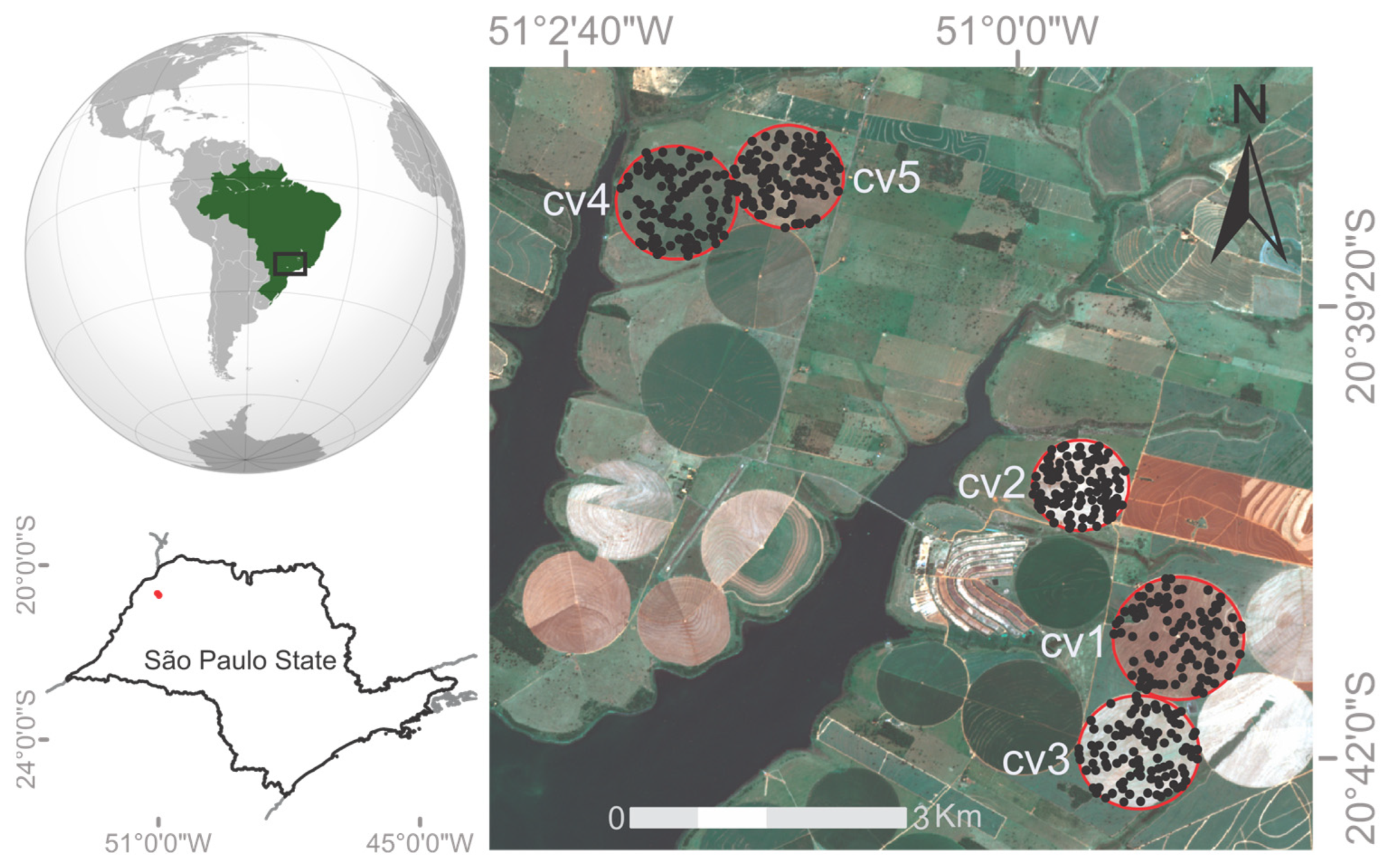
2.1. Experimental Area and Treatments Evaluated

The study area is located in the municipality of Pereira Barreto in the State of São Paulo at the mouth of the Tietê River. According to the Köppen classification, the region climate is tropical rain forest with summer rainfall and winter drought (Aw) [14]. Average temperatures are between 26.8 and 21.2 °C, average annual rainfall is 1128 mm, and the average altitude of the region is 347 m.

Aiming to set water availability parameters so that there is no influence of water deficit on the VIs, in view of the differentiation only of soybean cultivars and not of other external factors, data from irrigated areas were used, in which irrigation management allowed the supply of water necessary for the proper crop development over the cycle (Figure 1).

Data were collected from five irrigated central pivots and with the same sowing date in the 2015/2016 crop season. Each pivot was grown with a different cultivar, which consisted of the following materials: CV1—P98y12 RR, CV2—Desafio RR, CV3—M6410 IPRO, CV4—M7110 IPRO, and CV5—NA5909 RR (Figure 1).

2.2. Image Acquisition and Multispectral Models

A cloudless orbital image of the site was acquired from the Google Earth Engine platform. The image is already corrected at the top of the atmosphere, where the conversion from digital numbers to sensor radiation was applied to the linear transformation conversion, the solar elevation and the Earth-Sun distance [15] for 2015/2016. The image used was from the Landsat-8 satellite with the OLI sensor (USGS Landsat 8 Collection 1 Tier 1 and Real-Time data TOA Reflectance) available in the LANDSAT/LC08/C01/T1_RT_TOA catalog for 18 January 2016, on path/row 222/074. The spectral bands used in this study were B1 (0.43–0.45 µm), B2 (0.45–0.51 µm), B3 (0.53–0.59 µm), B4 (0.64–0.67 µm), B5 (0.85–0.88 µm), B6 (1.57–1.65 µm), B7 (2.11–2.29 µm), and B9 (1.36–1.38 µm), all with a spatial resolution of 30 m. Besides the isolated spectral bands, a total of 13 VIs were calculated, as described by

Table 1. Vegetation spectral models calculated from spectral bands obtained via Landsat 8 Collection 1 Tier 1 and real-time data TOA reflectance.

Vegetation Indices	Equations
AFRI1600 (Aerosol Free Vegetation Index 1600)	$\left(R{\lambda }_{nir}-0.66\ast \frac{R{\lambda }_{SWIR1}}{R{\lambda }_{nir}+0.66\ast R{\lambda }_{SWIR1}}\right)$
ARVI2 (Atmospherically Resistant Vegetation Index 2)	$-0.18+1.17\ast \left(\left(R{\lambda }_{nir}-R{\lambda }_{red}\right)/\left(R{\lambda }_{nir}+R{\lambda }_{red}\right)\right)$
ATSAVI (Ajusted Transformed Soil-Ajusted VI)	$1.22\ast \left[\frac{\left(R{\lambda }_{nir}-1.22\ast R{\lambda }_{red}-0.03\right)}{\left(1.22\ast R{\lambda }_{nir}+R{\lambda }_{red}-1.22\ast 0.03+0.08(1+{1.22}^2\right)}\right]$
EVI (Enhanced Vegetation Index)	$2.5\ast \left(\frac{R{\lambda }_{nir}-R{\lambda }_{red}}{\left(R{\lambda }_{nir}+6\ast R{\lambda }_{red}-7.5\ast R{\lambda }_{blue}\right)+1}\right)$
EVI2 (Enhanced Vegetation Index 2)	$2.5\ast \left(R{\lambda }_{nir}-R{\lambda }_{red}\right)/\left(R{\lambda }_{nir}+2.4\ast R{\lambda }_{red}+1\right)$
GNDVI (Green Normalized Difference Vegetation Index)	$\frac{\left(R{\lambda }_{nir}-R{\lambda }_{red}\right)}{\left(R{\lambda }_{nir}+R{\lambda }_{red}\right)}$
GRNDVI (Green-Red NDVI)	$[R{\lambda }_{nir}-\left(R{\lambda }_{green}+R{\lambda }_{red}\right)]/[R{\lambda }_{nir}+\left(R{\lambda }_{green}+R{\lambda }_{red}\right)$
GVI (Tasselled Capvegetation)	$-0.2848\ast R{\lambda }_{blue}-0.2435\ast R{\lambda }_{green}-0.5436\ast R{\lambda }_{red}+0.7243\ast R{\lambda }_{nir}+0.0840\ast R{\lambda }_{SWIR1}-0.1800\ast R{\lambda }_{SWIR2}$
GVMI (Global Vegetation Moisture Index)	$\frac{\left(R{\lambda }_{nir}+0.1\right)-\left(R{\lambda }_{SWIR2}+0.02\right)}{\left(R{\lambda }_{nir}+0.1\right)-\left(R{\lambda }_{SWIR2}+0.02\right)}$
MNDVI (Modified Normalized Difference Vegetation Index)	$\frac{\left(R{\lambda }_{nir}-R{\lambda }_{SWIR2}\right)}{\left(R{\lambda }_{nir}+R{\lambda }_{SWIR2}\right)}$
NDVI (Normalized Difference Vegetation Index)	$\frac{\left(R{\lambda }_{nir}-R{\lambda }_{red}\right)}{\left(R{\lambda }_{nir}+R{\lambda }_{red}\right)}$
SBI (Tasselled Cap—brightness)	$0.3037\ast R{\lambda }_{blue}+0.2793\ast R{\lambda }_{green}+0.4743\ast R{\lambda }_{red}+0.5585\ast R{\lambda }_{nir}+0.5082\ast R{\lambda }_{Cirrus}+0.1863\ast R{\lambda }_{SWIR2}$
SIWSI (Normalized Difference 860/1640)	$\frac{\left(R{\lambda }_{nir}-R{\lambda }_{SWIR1}\right)}{\left(R{\lambda }_{nir}+R{\lambda }_{SWIR1}\right)}$

.

For data acquisition from the 100 random repetitions (pixel by pixel) per cultivar on the orbital image, the Google Colab platform was used in Python language through the packages ee, os, and geemap [16].

2.3. Using Machine Learning Models

The models tested were: artificial neural networks (ANN), radial basis function (RBF) network, the decision tree algorithms J48 (DT) and reduced error pruning (REPTree), random forest (RF), and support vector machine (SVM). The ANN tested consists of a single hidden layer formed by a number of neurons that is equal to the number of attributes, plus the number of classes, all divided by 2. The J48 algorithm (DT) is a classifier for generating a C4.5 decision tree with an additional pruning step based on reduced-error strategy [17,18]. RBF is a feed-forwarded network in which training is performed in a hidden layer, implementing a normalized Gaussian radial basis function and the k-means clustering algorithm for the basis function of this hidden layer, and supervised learning is used for the output layer [19]. REPTree uses the decision tree logic and creates several trees in different iterations. Afterwards, it selects the best tree using the information gain and performs the reduced-error pruning as splitting criterion [20]. The RF model is able to produce multiple decision trees for the same dataset and uses a voting scheme among all these learned trees to classify new instances [21]. SVM performs classification tasks by building hyperplanes in multidimensional space to distinguish different classes [22].

The classification of the five soybean cultivars was performed by the six ML models in a 10-fold stratified randomized cross-validation with ten repetitions (100 runs for each model). Different inputs were considered for each classification model: spectral bands only (SBs), vegetation indices only (VIs), and SBs + VIs. The parameters obtained for performance evaluation of the models and inputs were correct classification (CC, %) and Kappa coefficient. ML analyses were performed on Weka 3.9.4 software using the default setting for all tested models [23] using a CPU Intel^® CoreTM i5 with 6 Gb RAM.

2.4. Statistical Analysis

After obtaining the r and MAE parameters, analysis of variance was performed considering a 6 × 3 factorial scheme (models versus inputs) with ten repetitions (folds). The means were grouped by the Scott-Knott test at 5% probability. Bar graphs were generated for each parameter (r and MAE) considering the models and inputs tested. Based on these statistics, the best ML technique was identified, and a confusion matrix was developed for this technique and the different inputs evaluated. These analyses were performed on R software [24] using the packages ExpDes.pt and ggplot2.

3. Results

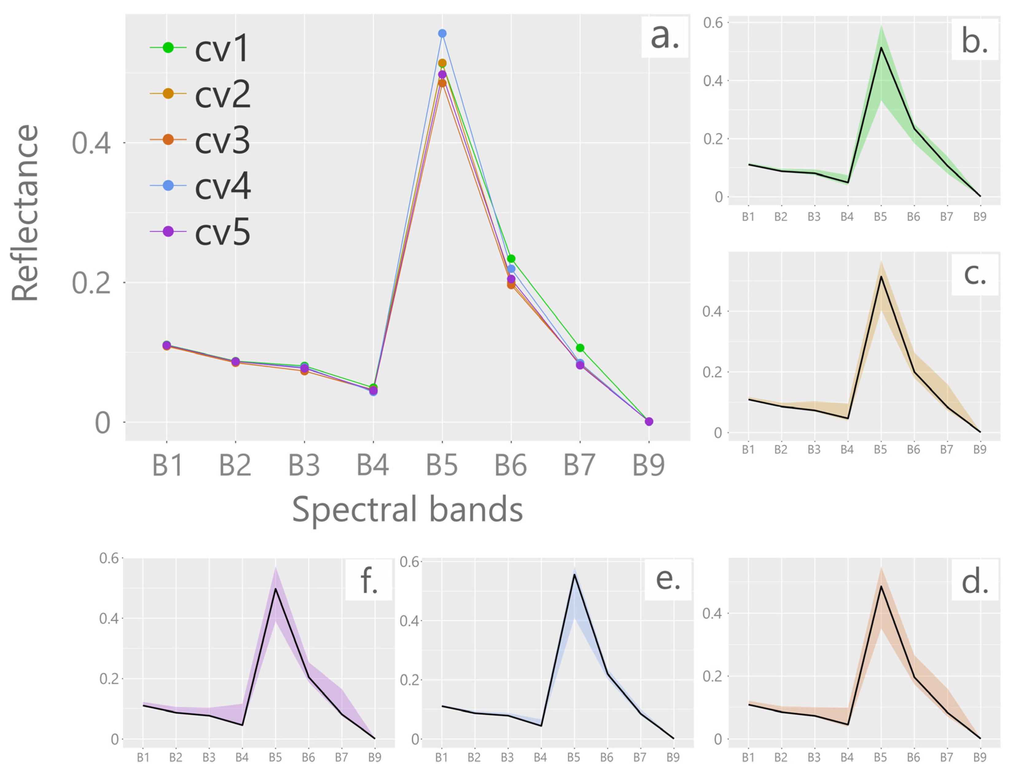
3.1. Spectral Signature of Cultivars

The result of the spectral curves extracted from the corrected Landsat-8/OLI TOA image for the 100 repetitions of each cultivar is represented in Figure 2. Visually, there is a slight difference between the spectral signatures for the five cultivars, considering the eight spectral bands analyzed. The variations occur more intensely when isolating each variety cultivar’s maximum and minimum values (Figure 2a–f).

The physiological appearance of the analyzed soybean cultivars (cv1 … cv5) as a function of the mean spectral curves (Figure 3a) is shown to be healthy, and can be noticed mainly by the high reflectance for B5 (~0.865 µm) and absorptions by B4 (~0.655 µm), B6 (~1.61 µm), and B7 (~2.2 µm).

The OLI sensor’s reflectance values for all cultivars were consistent compared to the target healthy green vegetation behavior. It is considered as collection data of the curves the day of the scene passage in January, which refers to the vegetative vigor of the soybean crop in the site studied, clearly in the phenological stage R5 (Figure 3).

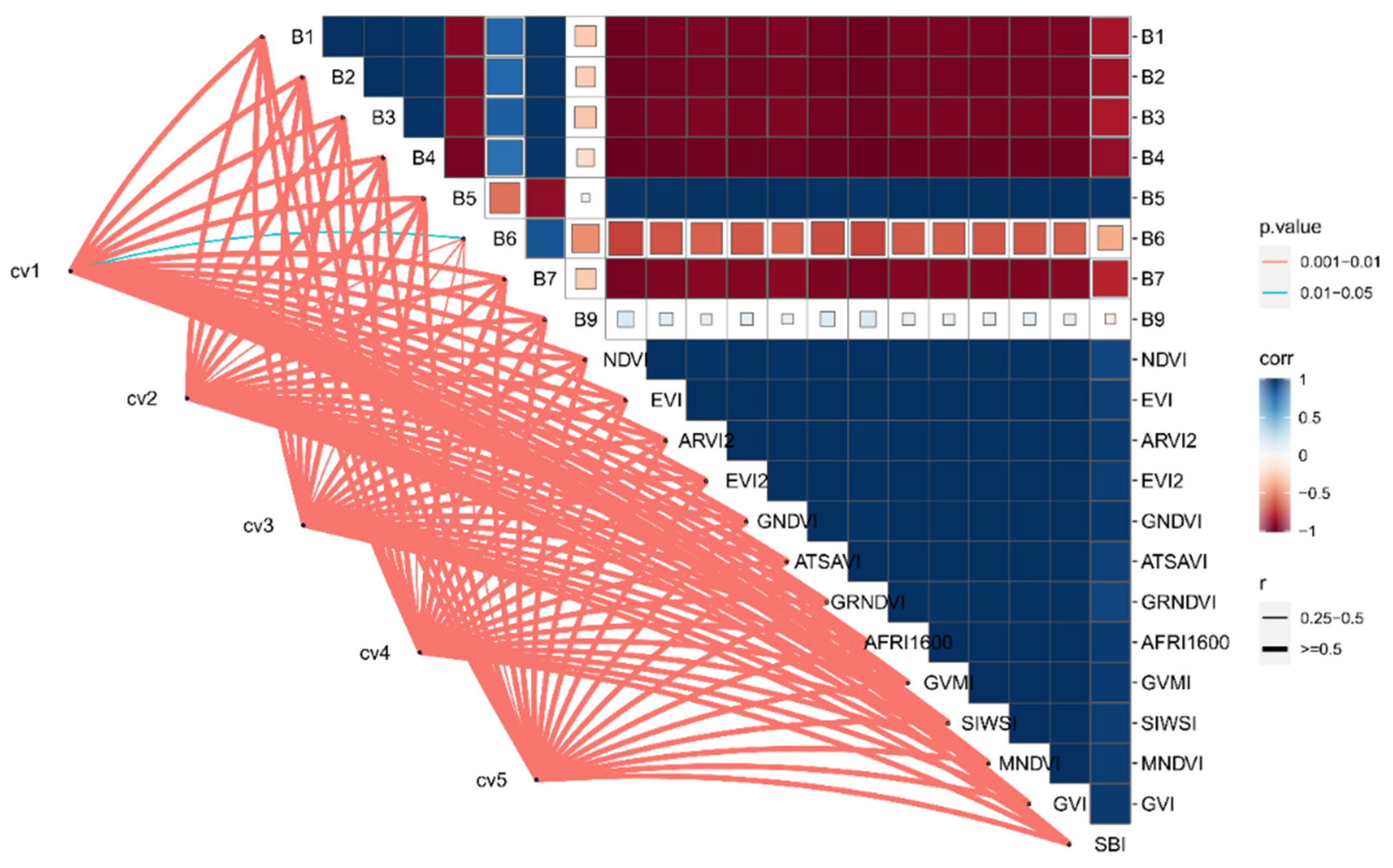
3.2. Correlation between Variables

Figure 4 demonstrates the correlogram between soybean cultivars and the spectral variables (SB and VIs) evaluated. It is possible to see that all variables were significantly related to the SB and VIs. The VIs showed a positive and high-magnitude correlation with each other. Bands B1, B2, B3, B4, B6, and B7 correlated positively with each other and negatively with all VIs. Band B5 correlated negatively with bands B1, B2, B3, B4, B6, and B7, and positively with all VIs. Band B9 showed negative low-magnitude correlations with the other bands and no correlation with the VIs.

3.3. Scattering between Variables

A scatterplot of the correct classification (%) and kappa coefficient for discrimination of five soybean cultivars using ML models and different inputs is shown in Figure 5. It can be seen that using ANNs with the inputs SB and SB + VIs gives the highest values of correct classification (%) and kappa coefficient for discriminating soybean cultivars. Using these same inputs, the random forest (RF) algorithm obtained values close to the ANNs but slightly inferior. It is important to highlight that regardless of the model and input tested, there was low variability between folds, occurring just one outlier in some cases.

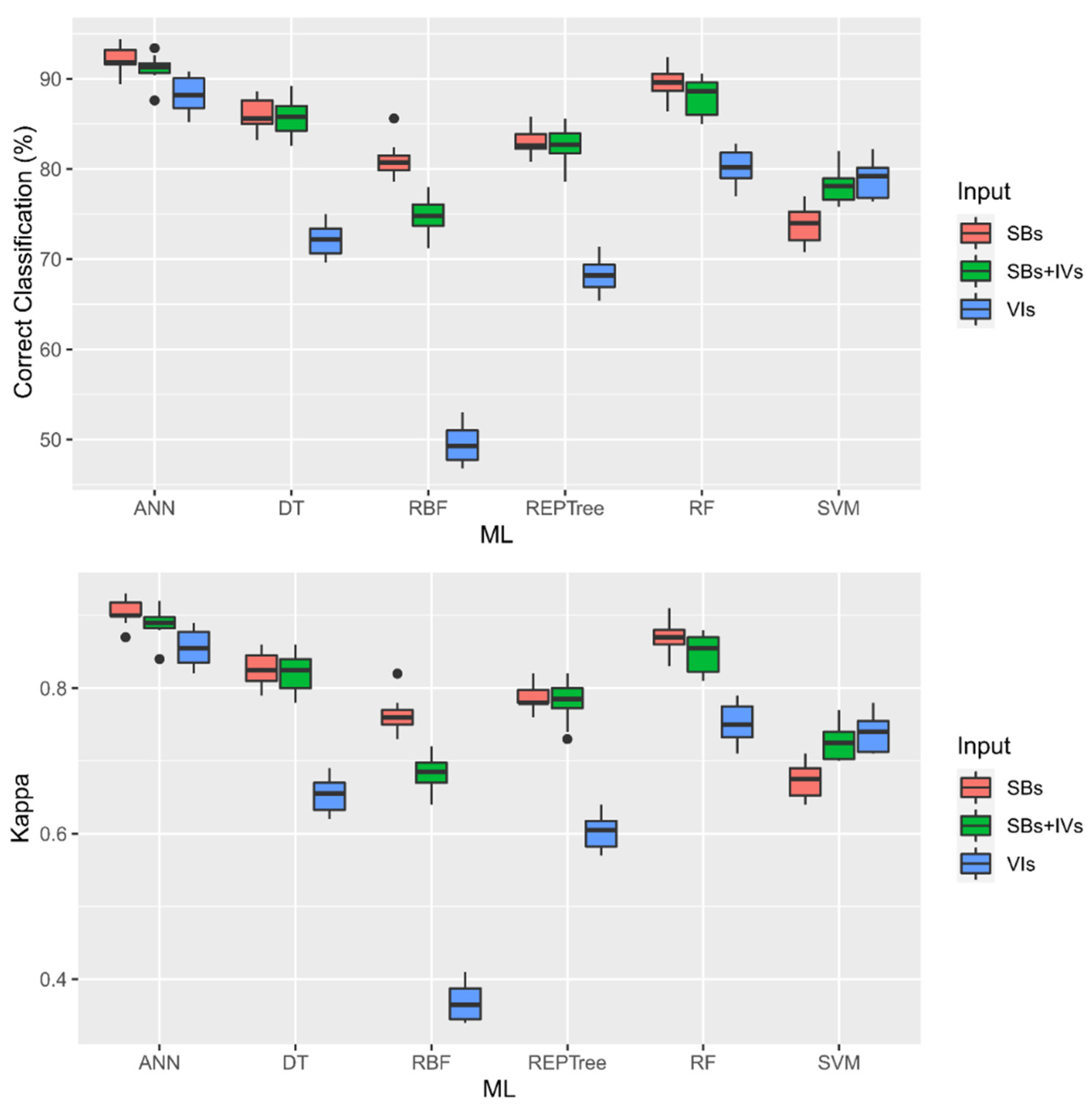
3.4. Choosing the Best Model and Best Input

The unfolding of the significant interaction between model x input for correct classification (%) and Kappa coefficient for discrimination of five soybean cultivars are shown in

Table 2. Unfolding of the significant model x input interaction for the correct classification (%) of five soybean cultivars using machine learning (ML) models and different inputs (vegetation indices—VIs, spectral bands—SBs, and SBs + VIs).

Model	SBs *	VIs	SBs + VIs
ANN	92.18 Aa	88.30 Ba	91.12 Aa
DT	85.88 Ac	72.24 Bc	85.72 Ac
RBF	80.94 Ab	49.50 Be	74.88 Af
REPTree	82.92 Ad	68.32 Bd	82.46 Ad
RF	89.62 Ae	80.22 Bb	87.94 Ab
SVM	73.82 Bf	78.86 Ab	78.24 Ae

* Means followed by equal lowercase letters in the same column and equal uppercase letters in the same row do not differ by the Scott–Knott test at 5% probability.

and

Table 3. Unfolding of the significant model × input interaction for the Kappa coefficient for discrimination of five soybean cultivars using machine learning (ML) models and different inputs (vegetation indices—VIs, spectral bands—SBs, and SBs + VIs).

Model	SBs *	VIs	SBs + VIs
ANN	0.91 Aa	0.86 Ba	0.89 Aa
DT	0.82 Ac	0.66 Bc	0.82 Ac
RBF	0.76 Ae	0.37 Ce	0.68 Bf
REPTree	0.79 Ad	0.60 Bd	0.78 Ad
RF	0.87 Ab	0.75 Bb	0.85 Ab
SVM	0.67 Bf	0.73 Ab	0.74 Ae

* Means followed by equal lowercase letters in the same column and equal uppercase letters in the same row do not differ by the Scott–Knott test at 5% probability.

, respectively. By analyzing the unfolding of models within input, ANNs presented the highest mean correct classification and Kappa coefficient regardless of the input used. For the input within model splitting, the spectral bands (SBs) and spectral bands + vegetation indices (SBs + VIs) inputs had the highest mean correct classifications and Kappa coefficients and did not differ for ANNs, DT, REPTree, and RF models.

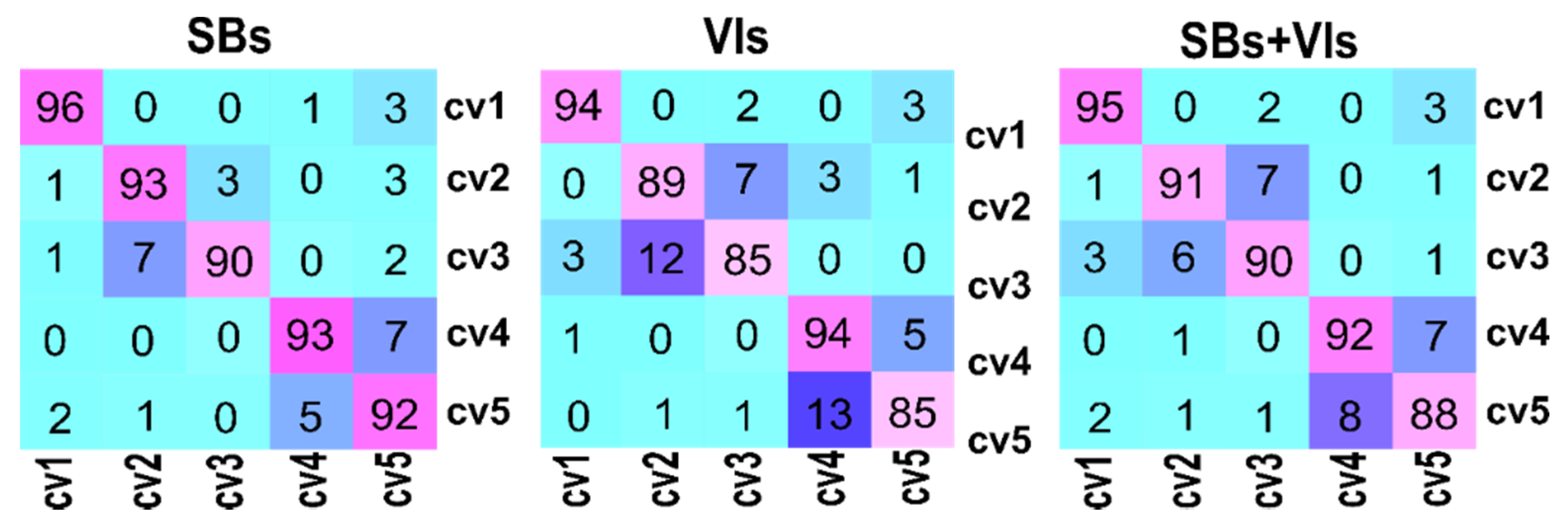
3.5. Confusion Matrix Using ANN’s

Based on the results contained in Table 2 and Table 3, the ANNs showed a better ability to discriminate soybean cultivars. Thus, Figure 6 shows the confusion matrix obtained with this model for each evaluated input. The diagonal (pink-scale values) shows the number of correct classifications obtained for each cultivar. It can be seen that using SBs and SBs + VIs as inputs provides the highest number of correct classifications. These inputs showed no statistical difference between them (see Table 2 and Table 3) and were superior to using VIs as input.

4. Discussion

4.1. Tested Models

Using machine learning has innovative potential in any area of science. The basic requirement is that there must be enough data to train and validate the tested models, making a considerable amount of data necessary [25]. Among the models tested, the ANNs stood out for achieving higher means of correct classification and Kappa coefficient, being the most accurate among the evaluated models in identifying soybean cultivars. Using data derived from spectral images, Eugenio et al. [26] reached an adequate adjustment and generalization capacity using ANNs to predict soybean yield. The modeling used by ANNs can achieve high accuracy, leading to answers to cover several situations [27].

In some studies, the use of ANN has provided more reliable results than other modeling techniques [28], such as Stepwise Multiple Linear Regression (MLR) and Principal Component Regression (PCR) [29]. The ANNs are also a more accurate alternative in predicting crop yields than traditional regression models [30].

Taratuhin et al. [31] found high accuracy using ANNs in predicting the earliness of the soybean accesses. Taratuhin et al. [32] found high accuracy in modeling using ANN in predicting several traits of soybeans under different climatic conditions. In eucalyptus, it is widely used to estimate yield since adopting traditional methods is difficult due to the number of independent variables and the complex relationship between them and the dependent variable [33].

Using ANNs together with spectral bands and/or vegetation indices generates accurate results in providing information about forest inventories with time and labor savings, since they have the ability to learn and present information about non-linear data [34]. These coupled techniques successfully improve accuracy, speed, and reliability in several research lines, as well as to farmers [35].

4.2. Tested Inputs

The use of remote sensing for measuring soybean agronomic traits has great potential to revolutionize genetic breeding programs and production systems, especially because this technology allows the quantification of phenotypic variables by combining images [10]. Traditional genotype selection programs are limited to costly and imprecise field analyses, which can be improved using remote sensing technologies [5]. This technology demonstrates efficiency in classifying soybean varieties, as previously reported by Silva Junior et al. [7,36].

When evaluating the inputs within each model, SBs and SBs + VIs obtained the highest means for correct classification and Kappa coefficient. Even though both inputs have achieved similar results, in a practical way, using the SBs would be more feasible since to obtain them, it is not necessary to perform calculations such as those used in the acquisition of the VIs.

Spectral bands are a reliable source for spatial and temporal detailing, making estimates on variables such as chlorophyll and leaf area index in agricultural crops [37]. Silva Junior et al. [38] have achieved accurate responses using spectral bands in discriminating eucalyptus plants for different levels of boron fertilization.

In addition to the results exposed in the breakdowns for correct classification and Kappa coefficient, the correlogram showed a significant relationship between spectral bands and variables. These results demonstrate the efficiency of using the spectral bands B1, B2, B3, B4, B6, and B7 to identify soybean cultivars. Using more than one spectral band when processing the analyses, a detailed exploration of what is being evaluated is possible, providing relevant information about the differentiation of soybean varieties [7,39].

Table 2 and Table 3 show the efficiency of using spectral bands with artificial neural networks, which is highlighted by the results presented by the confusion matrix (Figure 5). Using methodologies that evaluate the plant phenotype associated with computational intelligence is an accurate and reliable way to measure characteristics when the crop is still in the field [40].

Our findings demonstrate that it is possible to distinguish soybean genotypes more accurately using spectral bands as input in the tested machine learning models. This represents an important scientific advance for mapping soybean areas in world. For example, in Brazil, a large number of soybean cultivars are used annually, which have several different characteristics from each other, especially regarding the cycle. As in Brazil, soybean is grown in the crop season, being able to distinguish soybean cultivars demonstrates the possibility of introducing public policies for the prevention of end-of-cycle diseases, harvest planning and off-season planting.

However, it is also necessary that more orbital data be evaluated in the discrimination of plant species, seeking to achieve the absence of clouds, either through data with better spatial resolution (Sentinel-2/MSI) or even via satellite constellations (PlanetScope). Possibly the application of machine learning techniques can bring new results with the different characteristics of the various orbital sensors, even those that are equivalent, as is the case of the new Landsat-9 platform [41].

5. Conclusions

Spectral bands were the most accurate among the tested inputs in identifying soybean cultivars. Artificial neural networks provided the highest accuracy in identifying soybean cultivars. These findings demonstrate that it is possible to distinguish soybean genotypes more accurately using spectral bands using public images (Landsat-8 satellite) as input in the tested machine learning models. This represents an advance in soybean mapping, allowing us to accurately identify the most planted cultivars in a given region. However, it is also necessary that more orbital data be evaluated in the discrimination of plant species, seeking to achieve the absence of clouds, either through data with better spatial resolution (Sentinel-2/MSI) or even via satellite constellations (PlanetScope).

References

1. Maher, T.M.; Spagnolo, P. Perspectives for the Future. ERS Monogr. 2016, 2016, 260–274. [Google Scholar] [CrossRef]
2. Dukhnytskyi, B. World Agricultural Production. Ekon. APK 2019, 7, 59–65. [Google Scholar] [CrossRef]
3. SojaMaps: Monitoring of Soybean Areas through Satellite Imagery. Available online: https://pesquisa.unemat.br/gaaf/plataformas/sojamaps (accessed on 15 May 2022).
4. da Silva Junior, C.A.; Leonel-Junior, A.H.S.; Rossi, F.S.; Correia Filho, W.L.F.; de Barros Santiago, D.; de Oliveira-Júnior, J.F.; Teodoro, P.E.; Lima, M.; Capristo-Silva, G.F. Mapping Soybean Planting Area in Midwest Brazil with Remotely Sensed Images and Phenology-Based Algorithm Using the Google Earth Engine Platform. Comput. Electron. Agric. 2020, 169, 105194. [Google Scholar] [CrossRef]
5. Zhou, S.; Mou, H.; Zhou, J.; Zhou, J.; Ye, H.; Nguyen, H.T. Development of an Automated Plant Phenotyping System for Evaluation of Salt Tolerance in Soybean. Comput. Electron. Agric. 2021, 182, 106001. [Google Scholar] [CrossRef]
6. Diao, C. Remote Sensing Phenological Monitoring Framework to Characterize Corn and Soybean Physiological Growing Stages. Remote Sens. Environ. 2020, 248, 111960. [Google Scholar] [CrossRef]
7. da Silva Junior, C.A.; Nanni, M.R.; Shakir, M.; Teodoro, P.E.; de Oliveira-Júnior, J.F.; Cezar, E.; de Gois, G.; Lima, M.; Wojciechowski, J.C.; Shiratsuchi, L.S. Soybean Varieties Discrimination Using Non-Imaging Hyperspectral Sensor. Infrared Phys. Technol. 2018, 89, 338–350. [Google Scholar] [CrossRef]
8. Santana, D.C.; Cotrim, M.F.; Flores, M.S.; Rojo Baio, F.H.; Shiratsuchi, L.S.; da Silva Junior, C.A.; Teodoro, L.P.R.; Teodoro, P.E. UAV-Based Multispectral Sensor to Measure Variations in Corn as a Function of Nitrogen Topdressing. Remote Sens. Appl. Soc. Environ. 2021, 23, 100534. [Google Scholar] [CrossRef]
9. Feng, L.; Chen, S.; Zhang, C.; Zhang, Y.; He, Y. A Comprehensive Review on Recent Applications of Unmanned Aerial Vehicle Remote Sensing with Various Sensors for High-Throughput Plant Phenotyping. Comput. Electron. Agric. 2021, 182, 106033. [Google Scholar] [CrossRef]
10. Zhou, J.; Zhou, J.; Ye, H.; Ali, M.L.; Chen, P.; Nguyen, H.T. Yield Estimation of Soybean Breeding Lines under Drought Stress Using Unmanned Aerial Vehicle-Based Imagery and Convolutional Neural Network. Biosyst. Eng. 2021, 204, 90–103. [Google Scholar] [CrossRef]
11. van Dijk, A.D.J.; Kootstra, G.; Kruijer, W.; de Ridder, D. Machine Learning in Plant Science and Plant Breeding. iScience 2021, 24, 101890. [Google Scholar] [CrossRef]
12. Marques Ramos, A.P.; Prado Osco, L.; Elis Garcia Furuya, D.; Nunes Gonçalves, W.; Cordeiro Santana, D.; Pereira Ribeiro Teodoro, L.; Antonio da Silva Junior, C.; Fernando Capristo-Silva, G.; Li, J.; Henrique Rojo Baio, F.; et al. A Random Forest Ranking Approach to Predict Yield in Maize with Uav-Based Vegetation Spectral Indices. Comput. Electron. Agric. 2020, 178, 105791. [Google Scholar] [CrossRef]
13. Schwalbert, R.A.; Amado, T.; Corassa, G.; Pott, L.P.; Prasad, P.V.V.; Ciampitti, I.A. Satellite-Based Soybean Yield Forecast: Integrating Machine Learning and Weather Data for Improving Crop Yield Prediction in Southern Brazil. Agric. For. Meteorol. 2020, 284, 107886. [Google Scholar] [CrossRef]
14. Alvares, C.A.; Stape, J.L.; Sentelhas, P.C.; De Moraes Gonçalves, J.L.; Sparovek, G. Köppen’s Climate Classification Map for Brazil. Meteorol. Z. 2013, 22, 711–728. [Google Scholar] [CrossRef]
15. Chander, G.; Markham, B.L.; Helder, D.L. Summary of Current Radiometric Calibration Coefficients for Landsat MSS, TM, ETM+, and EO-1 ALI Sensors. Remote Sens. Environ. 2009, 113, 893–903. [Google Scholar] [CrossRef]
16. Wu, Q. Geemap: A Python Package for Interactive Mapping with Google Earth Engine. J. Open Source Softw. 2020, 5, 2305. [Google Scholar] [CrossRef]
17. Al Snousy, M.B.; El-Deeb, H.M.; Badran, K.; Khlil, I.A. Al Suite of Decision Tree-Based Classification Algorithms on Cancer Gene Expression Data. Egypt. Inform. J. 2011, 12, 73–82. [Google Scholar] [CrossRef] [Green Version]
18. da Silva, C.A., Jr.; Nanni, M.R.; de Oliveira-Júnior, J.F.; Cezar, E.; Teodoro, P.E.; Delgado, R.C.; Shiratsuchi, L.S.; Shakir, M.; Chicati, M.L. Object-Based Image Analysis Supported by Data Mining to Discriminate Large Areas of Soybean. Int. J. Digit. Earth 2018, 12, 270–292. [Google Scholar] [CrossRef]
19. Soni, R.; Kumar, B.; Chand, S. Optimal Feature and Classifier Selection for Text Region Classification in Natural Scene Images Using Weka Tool. Multimed. Tools Appl. 2019, 78, 31757–31791. [Google Scholar] [CrossRef]
20. Kalmegh, S.R. Analysis of WEKA Data Mining Algorithm REPTree, Simple Cart and RandomTree for Classification of Indian News. Int. J. Innov. Sci. Eng. Technol. 2015, 2, 438–446. [Google Scholar]
21. Belgiu, M.; Drăguţ, L. Random Forest in Remote Sensing: A Review of Applications and Future Directions. ISPRS J. Photogramm. Remote Sens. 2016, 114, 24–31. [Google Scholar] [CrossRef]
22. Nitin Rajvanshi, K.R. Chowdhary, Comparison of SVM and Naïve Bayes Text Classification Algorithms Using WEKA. Int. J. Eng. Res. 2017, V6, 141–143. [Google Scholar] [CrossRef]
23. Bouckaert, R.R.; Frank, E.; Hall, M.A.; Holmes, G.; Pfahringer, B.; Reutemann, P.; Witten, I.H. WEKA—Experiences with a Java Open-Source Project. J. Mach. Learn. Res. 2010, 11, 2533–2541. [Google Scholar]
24. R Core Team. R: A Language and Environment for Statistical Computing. Available online: http://softlibre.unizar.es/manuales/aplicaciones/r/fullrefman.pdf (accessed on 16 May 2022).
25. Montesinos-López, O.A.; Montesinos-López, A.; Pérez-Rodríguez, P.; Barrón-López, J.A.; Martini, J.W.R.; Fajardo-Flores, S.B.; Gaytan-Lugo, L.S.; Santana-Mancilla, P.C.; Crossa, J. A Review of Deep Learning Applications for Genomic Selection. BMC Genom. 2021, 22, 19. [Google Scholar] [CrossRef] [PubMed]
26. Eugenio, F.C.; Grohs, M.; Venancio, L.P.; Schuh, M.; Bottega, E.L.; Ruoso, R.; Schons, C.; Mallmann, C.L.; Badin, T.L.; Fernandes, P. Estimation of Soybean Yield from Machine Learning Techniques and Multispectral RPAS Imagery. Remote Sens. Appl. Soc. Environ. 2020, 20, 100397. [Google Scholar] [CrossRef]
27. Moradi, G.R.; Dehghani, S.; Khosravian, F.; Arjmandzadeh, A. The Optimized Operational Conditions for Biodiesel Production from Soybean Oil and Application of Artificial Neural Networks for Estimation of the Biodiesel Yield. Renew. Energy 2013, 50, 915–920. [Google Scholar] [CrossRef]
28. Badura, A.; Krysiński, J.; Nowaczyk, A.; Buciński, A. Prediction of the Antimicrobial Activity of Quaternary Ammonium Salts against Staphylococcus Aureus Using Artificial Neural Networks. Arab. J. Chem. 2021, 14, 103233. [Google Scholar] [CrossRef]
29. Ghasemi, G.; Nemati-Rashtehroodi, A. QSAR Modellemesi Ile Benzimidazole Türevlerinin Trikomoniasis Için Etkili Inhibitörler Olarak Kullanılması. Turk. J. Biochem. 2015, 40, 492–499. [Google Scholar] [CrossRef]
30. Basir, M.S.; Chowdhury, M.; Islam, M.N.; Ashik-E-Rabbani, M. Artificial Neural Network Model in Predicting Yield of Mechanically Transplanted Rice from Transplanting Parameters in Bangladesh. J. Agric. Food Res. 2021, 5, 100186. [Google Scholar] [CrossRef]
31. Taratuhin, O.D.; Novikova, L.Y.; Seferova, I.V.; Kozlov, K.N. Simulation of Soybean Phenology with the Use of Artificial Neural Networks. Biophysics 2019, 64, 440–447. [Google Scholar] [CrossRef]
32. Taratuhin, O.D.; Novikova, L.Y.; Seferova, I.V.; Gerasimova, T.V.; Nuzhdin, S.V.; Samsonova, M.G.; Kozlov, K.N. An Artificial Neural Network Model to Predict the Phenology of Early-Maturing Soybean Varieties from Climatic Factors. Biophysics 2020, 65, 106–117. [Google Scholar] [CrossRef]
33. de Freitas, E.C.S.; de Paiva, H.N.; Neves, J.C.L.; Marcatti, G.E.; Leite, H.G. Modeling of Eucalyptus Productivity with Artificial Neural Networks. Ind. Crops Prod. 2020, 146, 112149. [Google Scholar] [CrossRef]
34. Borges, M.V.V.; de Oliveira Garcia, J.; Batista, T.S.; Silva, A.N.M.; Baio, F.H.R.; da Silva Junior, C.A.; de Azevedo, G.B.; de Oliveira Sousa Azevedo, G.T.; Teodoro, L.P.R.; Teodoro, P.E. High-Throughput Phenotyping of Two Plant-Size Traits of Eucalyptus Species Using Neural Networks. J. For. Res. 2022, 33, 591–599. [Google Scholar] [CrossRef]
35. Singh, A.; Jones, S.; Ganapathysubramanian, B.; Sarkar, S.; Mueller, D.; Sandhu, K.; Nagasubramanian, K. Challenges and Opportunities in Machine-Augmented Plant Stress Phenotyping. Trends Plant Sci. 2021, 26, 53–69. [Google Scholar] [CrossRef] [PubMed]
36. da Silva Junior, C.A.; Teodoro, L.P.R.; Teodoro, P.E.; Baio, F.H.R.; de Andrea Pantaleão, A.; Capristo-Silva, G.F.; Facco, C.U.; de Oliveira-Júnior, J.F.; Shiratsuchi, L.S.; Skripachev, V.; et al. Simulating Multispectral MSI Bandsets (Sentinel-2) from Hyperspectral Observations via Spectroradiometer for Identifying Soybean Cultivars. Remote Sens. Appl. Soc. Environ. 2020, 19, 100328. [Google Scholar] [CrossRef]
37. Houborg, R.; Boegh, E. Mapping Leaf Chlorophyll and Leaf Area Index Using Inverse and Forward Canopy Reflectance Modeling and SPOT Reflectance Data. Remote Sens. Environ. 2008, 112, 186–202. [Google Scholar] [CrossRef]
38. da Silva Junior, C.A.; Teodoro, P.E.; Teodoro, L.P.R.; Della-Silva, J.L.; Shiratsuchi, L.S.; Baio, F.H.R.; Boechat, C.L.; Capristo-Silva, G.F. Is It Possible to Detect Boron Deficiency in Eucalyptus Using Hyper and Multispectral Sensors? Infrared Phys. Technol. 2021, 116, 103810. [Google Scholar] [CrossRef]
39. Ravikanth, L.; Jayas, D.S.; White, N.D.G.; Fields, P.G.; Sun, D.-W. Extraction of Spectral Information from Hyperspectral Data and Application of Hyperspectral Imaging for Food and Agricultural Products. Food Bioprocess Technol. 2017, 10, 1–33. [Google Scholar] [CrossRef]
40. Jung, J.; Maeda, M.; Chang, A.; Bhandari, M.; Ashapure, A.; Landivar-Bowles, J. The Potential of Remote Sensing and Artificial Intelligence as Tools to Improve the Resilience of Agriculture Production Systems. Curr. Opin. Biotechnol. 2021, 70, 15–22. [Google Scholar] [CrossRef]
41. USGS. Landsat 9 Data Users Handbook. Landsat 9 Data Users Handb. 2022, 107, 102689. [Google Scholar]
Figure 1. Location of areas cultivated with soybean cultivars in central pivot systems in southeastern Brazil. Each point represents the repetitions used (pixel by pixel).
Sustainability 14 07125 g001
Figure 2. Average spectral behavior of the five soybean cultivars (a) and their isolated minimum and maximum reflectances (P98y12 RR—cv1 (b), Desafio RR—cv2 (c), M6410 IPRO—cv3 (d), M7110 IPRO—cv4 (e), and NA5909 RR—cv5 (f)).
Sustainability 14 07125 g002
Figure 3. Vegetation indices calculated for the five cultivars (cv) evaluated using monotemporal OLI/Landsat-8 images.
Sustainability 14 07125 g003
Figure 4. Correlogram between different spectral bands and vegetation indices evaluated on five soybean cultivars (P98y12 RR—cv1; Desafio RR—cv2; M6410 IPRO—cv3; M7110 IPRO—cv4; NA5909 RR—cv5).
Sustainability 14 07125 g004
Figure 5. Boxplot for the variables correct classification (%) and Kappa coefficient for discrimination of five soybean cultivars using machine learning (ML) models and different inputs (vegetation indices—VIs, Spectral bands—SBs and SBs + VIs).
Sustainability 14 07125 g005
Figure 6. Confusion matrix for discrimination of five soybean cultivars using artificial neural networks (ANNs) and different inputs (vegetation indices—VIs, spectral bands—SBs, and SBs + VIs).
Sustainability 14 07125 g006