Can Water Price Improve Water Productivity? A Water-Economic-Model-Based Study in Heihe River Basin, China

Abstract

Water demand management through price and market mechanisms is crucial for agricultural water management. However, how to set an appropriate agricultural water price remains unclear due to the uncertainty regarding the response of water demand to price changes and the complexity of the hydro-economic system. Thus, this study developed a water-economic model to examine both issues in the Heihe River Basin. The empirical results revealed that the basin’s agricultural water is currently price-inelastic, with a value of −0.26, but that at 0.27 yuan/m³, elasticity is gained. At this tipping point, water demand and economic output decline by up to 10.2% and 1.6%, respectively, while water productivity increases by 7.2%. It is noteworthy that the reallocation of water and land resources from agricultural sectors to non-agricultural sectors facilitated by a water price change is the main contributor towards water productivity improvement. This signifies the importance of managing water and land resources in an integrated framework to improve water productivity in the future. Our study contributes to the literature by suggesting that future policies for water-demand management should consider pricing that encourages water saving and the reallocation of water resources to high-value uses in order to increase water productivity.

1. Introduction

Most endorheic basins around the world have seriously deteriorated watershed ecosystems caused by the fiercer competition for water use between human and natural habitats [1]. Increasing water productivity is essential for harmonising human and ecological water use by mitigating water competition between different stakeholders [2,3]. Defined as the economic value generated by unilateral water application, the concept of water productivity links water resources with the economic system; it endows water with economic attributes by considering the allocation efficiency and opportunity cost of water resource utilisation [4,5]. With an improvement in water productivity, more water can be reclaimed from human society and restored to nature, leading to a more harmonious relationship between humans, water, and the ecosystem [6,7]. Therefore, it is essential to find a way to improve water productivity in endorheic river basins to realise the optimal allocation of water resources.

The lack of economic incentives is considered the major cause of low water productivity in agriculture. In fact, the underpricing of irrigation water is constantly cited as the primary cause of the overexploitation of water resources in endorheic river basins [8,9]. Although water price instruments based on market mechanisms have recently been prioritised, and there is agreement that reasonable price signals help regulate extensive water consumption and promote water conservation, previous studies on the effectiveness of irrigation water price leveraging are inconsistent [10,11,12]. There are conflicting opinions regarding the effectiveness of water price instruments for water saving in practice. Research has shown that a reasonable water price encourages farmers to adopt advanced irrigation technologies and adjust their planting structure to pursue higher economic returns [13,14,15]. In contrast, others argue that this water-saving effect is not obvious and that, instead, it leads to a loss of income for farmers and a lack of initiative in agricultural production [16,17,18]. These conflicting views reflect the complexity of the factors associated with the effectiveness of water price instruments and their subsequent economic influences. That is, there is still much uncertainty regarding the reaction of water demand to a change in water price.

Moreover, knowledge of the interactive mechanism of the water–human system guarantees the setting of an appropriate agricultural water price instrument. Together with labour and capital, water is an important primary factor of economic activities, and changes in water price can cause a chain effect within the economic system [19,20,21]. It is therefore essential to comprehensively evaluate the economic impact caused by water price changes, since such changes will not only affect water demand in the agricultural sector but will also further influence economic output, consumption, and income. Explaining the interactive mechanism between water allocation and economic development remains a significant challenge. Previous studies have examined the coupling relationship between water and the economic system through hydro-economic models such as linear programming models, input–output models, partial general equilibrium models, and computable general equilibrium (CGE) models [22,23,24]. These studies have quantitatively evaluated how water has been optimised in the process of economic production, allocation, and consumption [25,26]. As a powerful tool in socio-economic system analysis, the CGE model has been widely used in water resource management. By coupling water resources with the economic system, the CGE model can systematically and comprehensively evaluate the participation of water resources in the production, consumption, distribution and flow processes of the economic system. The prevalent and widely used models include the ORANI-G model, the global scale GTAP-W model, and the multi-regional TERM-H2O model [27,28,29]. The research scope includes but is not limited to water price reform, water resource reallocation schemes, water-use efficiency improvement, and industrialisation processes for water resource utilisation [30,31,32].

A major problem with the application of the CGE model in agricultural water management is the neglect of the difference in water demand elasticity between the agricultural and non-agricultural sectors. In fact, the price elasticity of water demand in the agricultural sector is generally lower than that in non-agricultural sectors [33]. Water is usually considered as a product or primary production factor in the CGE and PE models. Furthermore, water and land are essential production elements for generating economic development. The level of socio-economic development is restricted by how much land and water resources are available both locally and regionally. Determining the right level of agricultural water demand and the substitution elasticity of water and land are therefore critical to achieving more reliable simulation results. However, these issues are not taken seriously in most hydro-economic models. Therefore, we first innovatively considered and estimated the key parameters and then integrated them into the model.

Considering that the evidence for the effectiveness of agricultural water prices is inconclusive and that how to set an appropriate water price is still an unresolved research problem, this research focuses on the coupling relationship between water and the economic system and uses a water-economic model (WEM) to evaluate the impact of agricultural water price on water productivity. To fill the gaps mentioned above, this study (1) quantitatively illustrates the relationship between agricultural water price and price elasticity to determine the key turning point from inelastic to elastic; (2) proposes and develops a WEM to represent the integrated water–economy system by combining economic development and water management issues in a comprehensive framework based on a case study of the Heihe River Basin (HRB); and (3) uses the WEM to evaluate the impact of agricultural water price reform on regional water productivity so as to provide a theoretical basis for water price reform.

2. Study Area

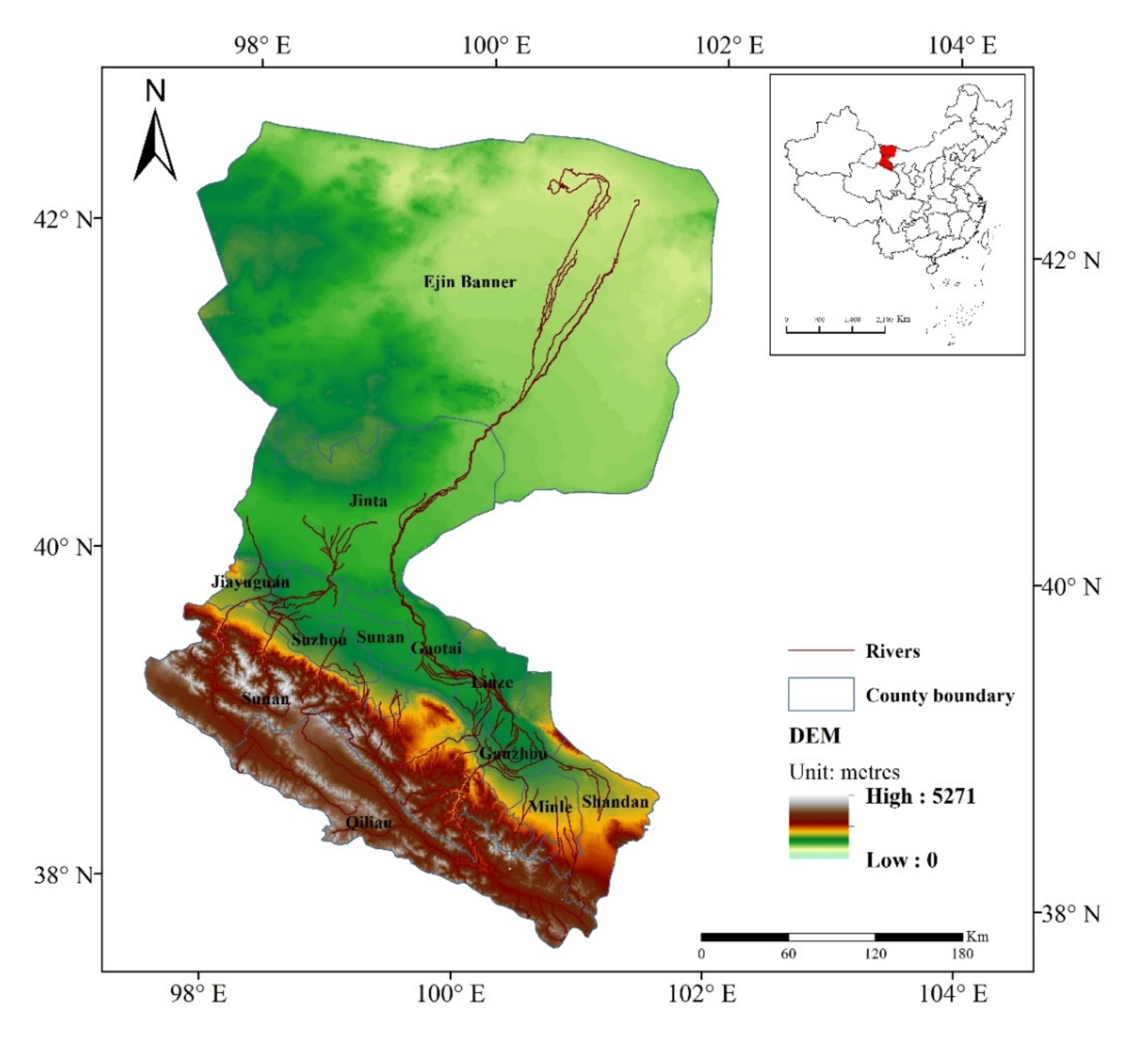
The HRB, a typical endorheic river basin in Northwest China (Figure 1), faces multiple difficulties, such as an undeveloped economy, water shortages, and a fragile eco-environment [1,34]. Economic development is seriously hampered by the scarcity of water resources, especially in the middle reaches of the basin, where the mismatch between water supply and water demand is prominent. There are five counties located in the middle reaches of HRB, which are Ganzhou District, Gaotai County, Linze County, Minle County, and Shandan County. The middle reach occupies 80% of the artificial oases and contributes 83% of the GDP of the basin. It also accounts for 95% of the cultivated land and 92% of the population in the basin. At present, the water resource utilisation in the middle reach is about 2.3 × 10⁹ m³, accounting for 61% of the total water consumption in the HRB, of which 94% is used in the agricultural sector. The utilisation efficiency of water resources is comparatively low, with a water consumption per CNY 10,000 GDP of 1736 m³, which is 1.85 times higher than the national average [35]. Due to the expansion of the oasis area, ecological water is increasingly being taken up by agricultural and industrial activities, thus causing a fragile ecological environment.

Notably, the agricultural water price is still low in the HRB, covering only 65% of the full operating cost of the conveyance system. Low water prices, on the one hand, lead to inefficient water supply services, and on the other hand, reduce the efficiency of water utilisation. Both academics and policymakers have realised that water price reform is one of the key management strategies for solving water disputes among different stakeholders. Therefore, in 2015, a pilot for an irrigation water price reform was launched in Gaotai County. However, the reform caused discontent among farmers. Some researchers have also expressed reservations about the water conservation effects and the economic influences of water price reform [16,36]. These negative attitudes necessitate the determination of the real effect and the underlying determinants of water price changes through a more comprehensive assessment. This study will also serve as a valuable reference for other endorheic river basins.

3. Model and Methodology

3.1. Framework of the Water-Economic Model

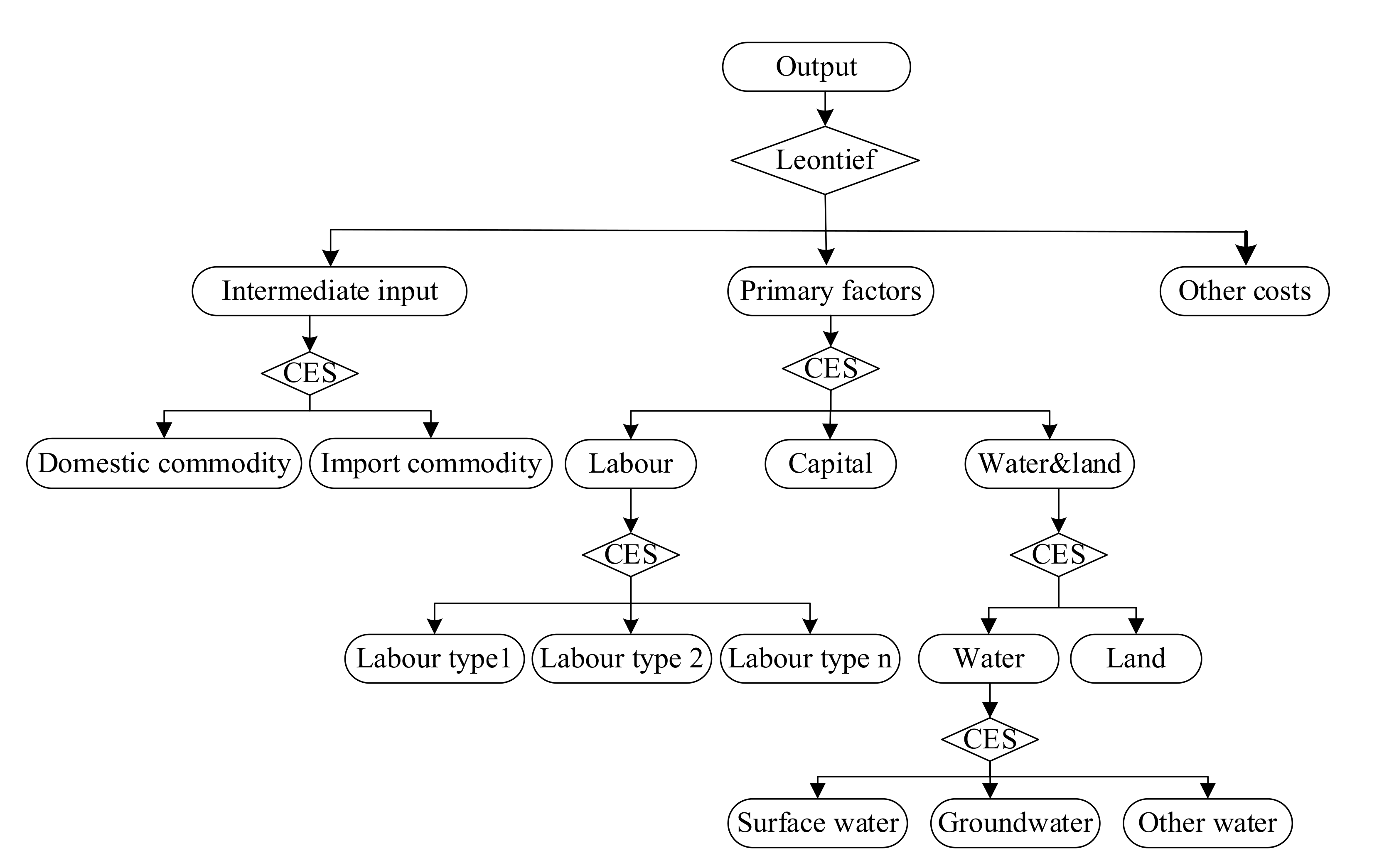
To systematically and comprehensively analyse the mutual feedback relationships between water resources and economic systems in the basin, this study develops a WEM that couples water resources with an economic system based on the computable general equilibrium (CGE) framework. The WEM is an economic system model based on the 2012 input/output table of Gaotai County [37,38]. It focuses on the interactions between water resources and economic elements. The WEM inherits all the functions of the CGE model and enhances the representations of the involvement of water and land in production processes, which plays a critical role in determining water allocations and land uses in the economic system [33]. The model includes 48 industrial sectors (

Table A1. Water used by different sectors in Gaotai county ($\times {10}^4{ \mathrm{m}}^3$ ).

Abbreviation	Sectors	Surface Water	Groundwater	“Other” Water
WHEAT	Wheat	3777.56	1834.66	44.20
CORN	Corn	12,540.53	5242.57	545.72
Oilseed	Oilseed	162.60	62.61	1.05
Cotton	Cotton	1360.41	679.67	4.15
Fruits	Fruits	4071.27	1397.99	158.00
Vegetables	Vegetables	6479.26	2699.53	224.08
OtherAg	“Other” agriculture	562.30	177.51	3.83
CoalMineProc	Coal mining and washing	0	0	0
CrudeOilGas	Oil and gas extraction	0	0	0
FerrOre	Metal mining and dressing	0	0	0
NFerrOre	Non-metallic mining and dressing	0	123.58	2.23
FoodTobacco	Food manufacturing and tobacco processing	0	111.46	14.01
Textil	Textiles	0	0	0
ClothesShoes	Clothing, leather, and its products	0	0	0
Furniture	Wood processing and furniture manufacturing	0	2.69	0.11
CultureGoods	Paper printing and stationery manufacturing	0	0	0
PetrolRef	Petroleum processing, coking, and nuclear fuel processing	0	0	39.30
Chemistry	Chemical industry	0	0.57	0.15
NMtlMinPr	Non-metallic mineral products	0	7.76	0.44
MSmeltProc	Metal smelting and calendering	0	0	0
Mprod	Metal products	0	0	0
GeSplEqpNEC	General and special equipment manufacturing	0	0	0
TransEqp	Transportation equipment manufacturing	0	0	0
ElctronEqp	Electrical, mechanical, and equipment manufacturing	0	0	0
OthElecEqp	Computer and communication equipment manufacturing	0	0	0
OfficeEqp	Instrument and machinery manufacturing	0	0	0
ArtsCrafts	Other manufacturing	0	0	0
Scrap	Scrap products	0	0	0
ElecSteam	Production and supply of electricity and steam	0	3.02	17.18
GasSupply	Gas production and supply	0	0	0
WaterSupply	Water production and supply	76.25	284.44	0.74
Construction	Construction	0	0.50	4.10
TransWare	Transportation and warehousing	0	0.12	0.27
Post	Postal industry	0	0	0
ComputSrvc	Information transmission, computer services, and software	0	0	0.10
Trade	Wholesale and retail trade	0	0	0.11
Hotels	Accommodation and catering	0	0.19	3.44
Finance	Finance and insurance	0	0	0.24
RealEstate	Real estate	0	0	0.01
Leasing	Leasing and business services	0	0	0.32
Tourism	Tourism	0	0	0
TechSrvc	Scientific research	0	0.04	0.01
PublicSrvc	Public service	0	1.36	5.44
ResidentSrvc	Other social services	0	0	0.14
Education	Education	0	6.33	5.54
SocWelfare	Health, social security, and social welfare	0	10.69	4.12
ArtsFilmTV	Culture, sports, and entertainment	0	0	0.13
PublicAdmin	Public administration and social organisation	0	0.04	0.89

); 4 primary input factors (labour, capital, land, and water); and 6 economic entities (production, investment, residents, government, inventory, and other regions). According to the planting structure of the HRB, the agricultural sector is divided into seven sub-sectors: wheat, maize, oil seed, cotton, fruit, vegetable, and ‘other’ agriculture. Water resources are also divided into three categories: surface water, groundwater, and ‘other’ water. These are introduced into the CGE model as primary factors. Similar to other CGE models, the WEM model has three main modules (production, consumption, and market equilibrium) and an additional module referred to as the land and water resource allocation module.

In contrast to previous CGE models, along with labour and capital, water and land in the WEM are considered primary factors in the production process. Since several previous papers have systematically explained the economic theory and introduced the operational mechanism of the CGE modelling framework in environmental issues [27,28,33], this study focuses on the land and water resources module in water-economic modelling, which represents the allocation mechanism of water and land in economic activities. The production technology is represented by a quadruple-nested production function that is structured by a series of Leontief assumptions and constant elasticity of substitution (CES) nesting assumptions (Figure 2). At the top level, producers combine intermediate commodities, primary factors, and other costs to produce final products via the Leontief production function. At the second level, domestic and imported products are combined to form intermediate commodities, and the four main primary factors—water, land, capital, and labour—are aggregated. At the third level, a composite of different types of labour via CES production and a combination of land and water is determined by its substitution elasticity. At the bottom level, water is composed of different sources, including surface water, groundwater, and other water. Theoretically, producers combine land and water via a CES production function to produce a land and water aggregate that is further combined with labour and capital to form the economic output. The production process can be depicted with CES production functions in Equations (1)–(4):

$$\frac{XLA{B}_{i,d}}{XPRI{M}_{i,d}}=ala{b}_{i,d}\cdot {[\frac{PPRI{M}_{i,d}\cdot ala{b}_{i,d}}{PLA{B}_{i,d}}]}^{\sigma pri{m}_i}$$

(1)

$$\frac{XLW{T}_{i,d}}{XPRI{M}_{i,d}}=alw{t}_{i,d}\cdot {[\frac{PPRI{M}_{i,d}\cdot alw{t}_{i,d}}{PLN{D}_{i,d}}]}^{\sigma pri{m}_i}$$

(2)

$$\frac{XCA{P}_{i,d}}{XPRI{M}_{i,d}}=aca{p}_{i,d}\cdot {[\frac{PPRI{M}_{i,d}\cdot aca{p}_{i,d}}{PCA{P}_{i,d}}]}^{\sigma pri{m}_i}$$

(3)

$$\begin{array}{c}XPRI{M}_{i,d}\cdot PRI{M}_{i,d}=PLW{T}_{i,d}\cdot XLW{T}_{i,d}+\\ \hspace{1em}\hspace{1em}\hspace{1em}\hspace{1em}\hspace{1em}\hspace{1em}\hspace{1em}\hspace{1em}\hspace{1em}\hspace{1em}\hspace{1em}\hspace{1em}\hspace{1em}\hspace{1em}\hspace{1em}\hspace{1em}PLA{B}_{i,d}\cdot XLA{B}_{i,d}+XCA{P}_{i,d}\cdot PCA{P}_{i,d}\end{array}$$

(4)

where XLAB_i,d, XLWT_i,d, XCAP_i,d, and XPRIM_i,d are the number of primary input factors of labour, land and water aggregate, capital, and the aggregate of the three input factors in sector i of region d, respectively; PLAB_i,d, PLWT_i,d, PCAP_i,d, and PPRIM_i,d are the prices of the factors; and alab_i,d, alwt_i,d, and acap_i,d are the technical coefficients of the production function.

Water and land are primary factors in the production structure, and they are nested based on the constant elasticity of substitution (CES) function. The equation is as follows:

$$\left\{\begin{array}{c}Min{{\displaystyle \sum }}_{i=1}^{48}\left(PWA{T}_i*XWA{T}_i+PLN{D}_i*XLN{D}_i\right)\\ s.t.{{\displaystyle \sum }}_{i=1}^{48}{\left(XWA{T}_i^{{\mu }_{wl}}+XLN{D}_i^{d{\mu }_{wl}}\right)}^{1/{\mu }_{wl}}=XLWT\end{array}\right..$$

(5)

where $PWA{T}_i$ is the water price of sector i,$PLN{D}_i$ is the land rental rate of sector i,$XWA{T}_i$ and $XLN{D}_i$ are the demand for water and land of sector i, ${\mu }_{wl}$ is the substitution elasticity, and $XLWT$ is the composited demand for land and water.

Therefore, water and land allocation can be analysed under this framework. For example, a water price increase will lead to less water demand in agricultural production. Furthermore, given the CES relationships between land, water, capital, and labour, rising water prices will lead to a substitution in the factor market.

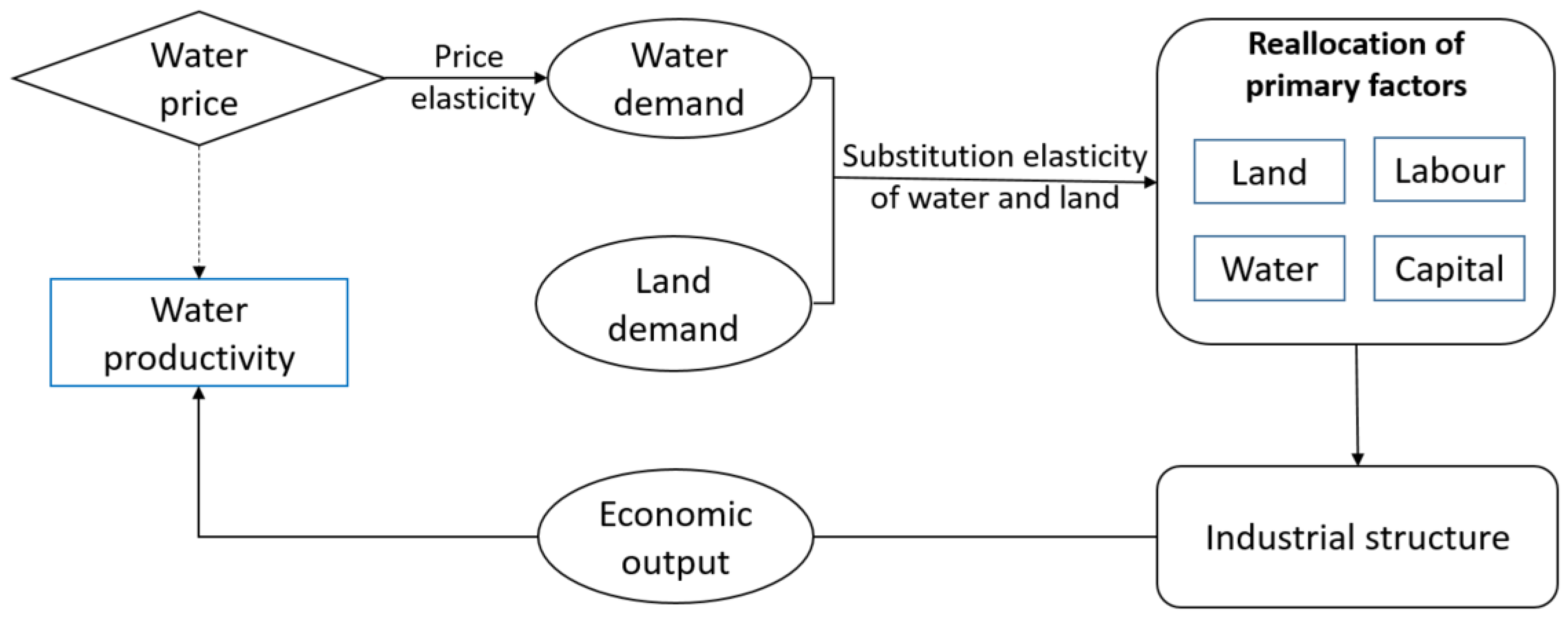
The WEM is a highly efficient tool for water resource management and policy decision support because it can explore the economic structure, feedback mechanism, and water flows among different sectors [19]. It can be used to simulate the chain effects among different sectors under different agricultural water price scenarios. The main interactive mechanism between water price and water productivity through the WEM is briefly expressed in Figure 3. A water price change will lead to water demand change, which will induce the reallocation of land and other input factors among industries. This will finally result in an economic output change and a change in water productivity. Two important parameters affect the entire process: water price elasticity and the substitution elasticity between water and land. The two parameters will be introduced in detail in Section 3.2 and Section 3.3, respectively.

The WEM was built based on the 2012 input–output table as the starting equilibrium point [33,37]. Water and land are incorporated in the input–output table as two different entities. The water entity is composed of two factors, the volume of water used by each sector and the price of water for each sector. The amount and price of water resources used by different industries were collected from the Water Resources Bulletin of Gansu Province and the General Survey of Water Resources. Combined with the field survey, the water resources utilisation data matched with the input–output table of 48 industries were calculated. Referring to the System of Environmental-Economic Accounting 2012 (SEEA 2012), this paper uses the net present value method and the market value method to calculate the value of land resources. Industrial land and residential land were calculated by the market price according to the average price of land bidding divided by its service life, with the service life of industrial land being 40 years and residential 70 years. Other non-agricultural land values were derived from the net present value method, which is the area multiplied by the land rent. The land area for each industry was obtained from a high-spatial-resolution remote-sensing land-use map combined with statistical data. The value of water resources and land resources are therefore embedded in the input–output table, which is the main database for the WEM. Under the condition of zero profit in a fully competitive market, the solution of the model equation system is based on the principle of supply balance, considering minimum cost and maximum utility.

3.2. Substitution Elasticity between Water and Land

In the WEM, a key parameter is the elasticity of substitution between water and land, which reflects the land and water allocation mechanism in the economic system [34]. It also reflects the possibility of dealing with water scarcity through economic transformation. The elasticity of substitution refers to the relative change in the input ratio caused by a relative change in the marginal technical substitution (MTS) rate under the condition that the technology level and input price remain unchanged [34]. Here, the elasticity of substitution between water and land can be represented as the ratio of marginal change of the input ratio of water and land resources and the marginal product of water and land. The principle of the elasticity parameter for water and land resources can be expressed as Equation (6):

$${\mu }_{WL}=\frac{\partial (WAT/LND)}{(WAT/LND)}/\frac{\partial (M{P}_{WAT}/M{P}_{LND})}{(M{P}_{WAT}/M{P}_{LND})}$$

(6)

The elasticity of water and land substitution is derived from the translog production function (TFP) model. Based on the TFP model, the elasticity of water and land substitution at each sample point can be calculated. The estimation process regarding the substitution elasticity of water and land resources based on the TFP model was detailed in [39]. When the elasticity is smaller than 1, it indicates that the change in the proportion of irrigation water and land is smaller than the change in the marginal product rate.

3.3. Price Elasticity of Agricultural Water Demand

The demand elasticity of the water price is used to measure the sensitivity degree of agricultural water demand to water prices. This is an important factor in guiding water price reform. The disparity between the elasticity of agricultural water demand and that of non-agricultural water demand is highly significant due to the price gap. To measure the elasticity of agricultural water demand, a quadratic production function was chosen to characterise the response of crop yield to irrigation, which was found to provide the best fit among irrigation decisions [40]. The water demand for crop i can be represented as:

$$w_i={\mu }^i+{\nu }^i{p}_i+{\displaystyle \sum _{v=1}^z{\omega }_v^i{r}_v+{\phi }^{i}wp+}{\vartheta }^i{n}_i+{\displaystyle \sum _{s=1}^{\iota }{\iota }_s^i{x}_s},i=1,\mathrm{\dots },m$$

(7)

where p_i is the sales price for crop i; r_v is the price of input factors except for water; wp is the price for irrigation water; n_i is the planting area of crop i; and x_s is other exogenous control variables including climate conditions, plot characteristics, soil conditions, irrigation technology, and household characteristics such as non-agricultural household income.

Therefore, the ratio of marginal crop water demand to marginal water price can be expressed as:

$$\frac{d{w}_i}{db}=\frac{\partial w_i}{\partial b}+\frac{\partial w_i}{\partial n_i^{*}}\cdot \frac{\partial n_i^{*}}{\partial wp}$$

(8)

Accordingly, the price elasticity of water demand can be obtained based on the transformation of the equation to the double-logarithm function. The price elasticity of irrigation water demand is, then, the regression coefficient of water price, which can be expressed as:

$${\xi }_i=(\frac{\partial w_i}{\partial wp}+\frac{\partial w_i}{\partial n_i^{*}}\cdot \frac{\partial n_i^{*}}{\partial wp})\cdot \frac{wp}{w_i}=[{\phi }^i+{\theta }^i({\delta }^i+{\lambda }_s^i{x}_s)]\cdot \frac{wp}{w_i},i=1,\mathrm{\dots },m$$

(9)

This represents the ratio of the percentage change in quantity demanded to the percentage change in the price of goods. When price elasticity is greater than 1, it indicates that water price is elastic and that an increasing water price will lead to significantly diminished water demand. The opposite is also true.

To analyse the relationship between elasticity and price, the marginal water-saving effect $\frac{\partial w_i}{\partial w{p}_i}$ of water price on crop i can be calculated according to the sample mean value of water price and water consumption. Then, the point elasticity ${\xi }_{ij}$ of crop i in plot j can be obtained based on the water price and water consumption of each sample plot:

$${\xi }_{ij}=\frac{\partial w_i}{\partial w{p}_i}\cdot \frac{w{p}_{ij}}{w_i}={\phi }^i\cdot \frac{w{p}_{ij}}{w_{ij}}$$

(10)

Site-specific agricultural production information including input and output data were collected through field survey in the middle reaches of the HRB [41]. Additionally, soil characteristics, climatic variables, and typical agronomic management practices were controlled in the model.

4. Results and Discussion

4.1. Estimation of Agricultural Water Price Elasticity

Table 1. Descriptive statistics of irrigation water demand and irrigation water price.

Price Interval	Surface Water		Groundwater		Irrigated with Both Surface Water and Groundwater
	Water Price	Amount	Water Price	Amount	Water Price	Amount
	(CNY/m³)	(m³/Mu)	(CNY/m³)	(m³/Mu)	(CNY/m³)	(m³/Mu)
Seed maize
Mean	0.12	724	0.11	430	0.12	810
1–25%	0.07	702	0.07	350	0.06	880
26–50%	0.1	790	0.12	560	0.11	838
51–75%	0.14	744	0.33	540	0.14	761
76–100%	0.21	551	0.5	240	0.22	630
Wheat
Mean	0.19	445	0.29	389	0.21	508
1–25%	0.08	610	0.08	540	0.08	696
26–50%	0.11	516	0.1	480	0.11	671
51–75%	0.14	500	0.22	400	0.14	483
76–100%	0.36	253	0.5	294	0.36	343
All crops
Mean	0.15	580	0.22	570	0.16	667
1–25%	0.08	666	0.08	515	0.07	783
26–50%	0.1	681	0.12	791	0.11	796
51–75%	0.14	625	0.18	605	0.15	621
76–100%	0.3	345	0.55	397	0.31	469

summarises the quartile statistics of irrigation water demand and prices. According to the range of irrigation water prices—that is, from low to high—the samples were divided into four equal parts, and the average irrigation water consumption in each price range was compared. The samples were separated into three categories (irrigated with surface water only, irrigated with groundwater only, and irrigated with both surface water and groundwater) based on different crop types, including maize, wheat, and ‘all crop’ samples. With a rise in water price, the consumption of surface irrigation water and groundwater shows a trend of first rising and then falling. The amount of water consumption decreases significantly from the third to the fourth price interval. The mean irrigation water used by all crops was 667 m³ per mu. The mean price for all samples was CNY 0.15 per m³ for surface water and CNY 0.22 per m³ for groundwater. A convexity relationship between irrigation water demand and irrigation water price can be found based on the sample statistics.

From the perspective of crops, on average, the water consumption of seed maize is higher than that of wheat, whereas the water cost per cubic metre of seed maize is lower than that of wheat. The mean total water fee for seed maize is CNY 0.12 per m³ with 810 m³ water applied and CNY 0.21 per m³ with 508 m³ water applied for wheat. Wheat is also more sensitive to water price change than seed maize. From the lowest to the highest price interval, water consumption by wheat decreased by 51%, while that by seed maize decreased by only 28%.

Water price elasticity, which measures the sensitivity of water demand to water price change, is an important indicator of how water demand responds to water price changes. The regression results of the irrigation water demand function showed the price elasticity of irrigation water demand to be fairly inelastic at −0.26 with a p-value of 0.009, which suggests that the estimate is reliable according to the irrigation water demand function (

Table 2. Estimation of irrigation water demand function.

Independent Variables	Dependent Variables
	Ln Water
Ln water_price	−0.260 ***
	(0.00996)
Ln seed	−0.215 ***
	(0.0717)
Ln seed_price	0.190 *
	(0.121)
Ln fertilizer_price	−0.146
	(0.177)
Ln dist_water	0.000160 *
	(8.57 × 10−5)
Ln area	0.00365 **
	(0.00524)
Affected by natural disaster or not	−0.00462
	(0.0707)
Drought resistant or not	0.0652
	(0.125)
Canal lining or not	0.211 *
	(0.110)
Constant	6.395 ***
	(0.424)
Samples	204
R-squared	0.306

Note: *, **, and *** represent significance levels at 1%, 5% and 10%, respectively.

). In other words, for every 1% increase in the value of the marginal products of water, the quantity of irrigation water demanded would decline by 0.26%. It should be mentioned that this result is in line with classical economic theories that demand for essential goods such as water can be categorised into inelastic or relatively inelastic demands.

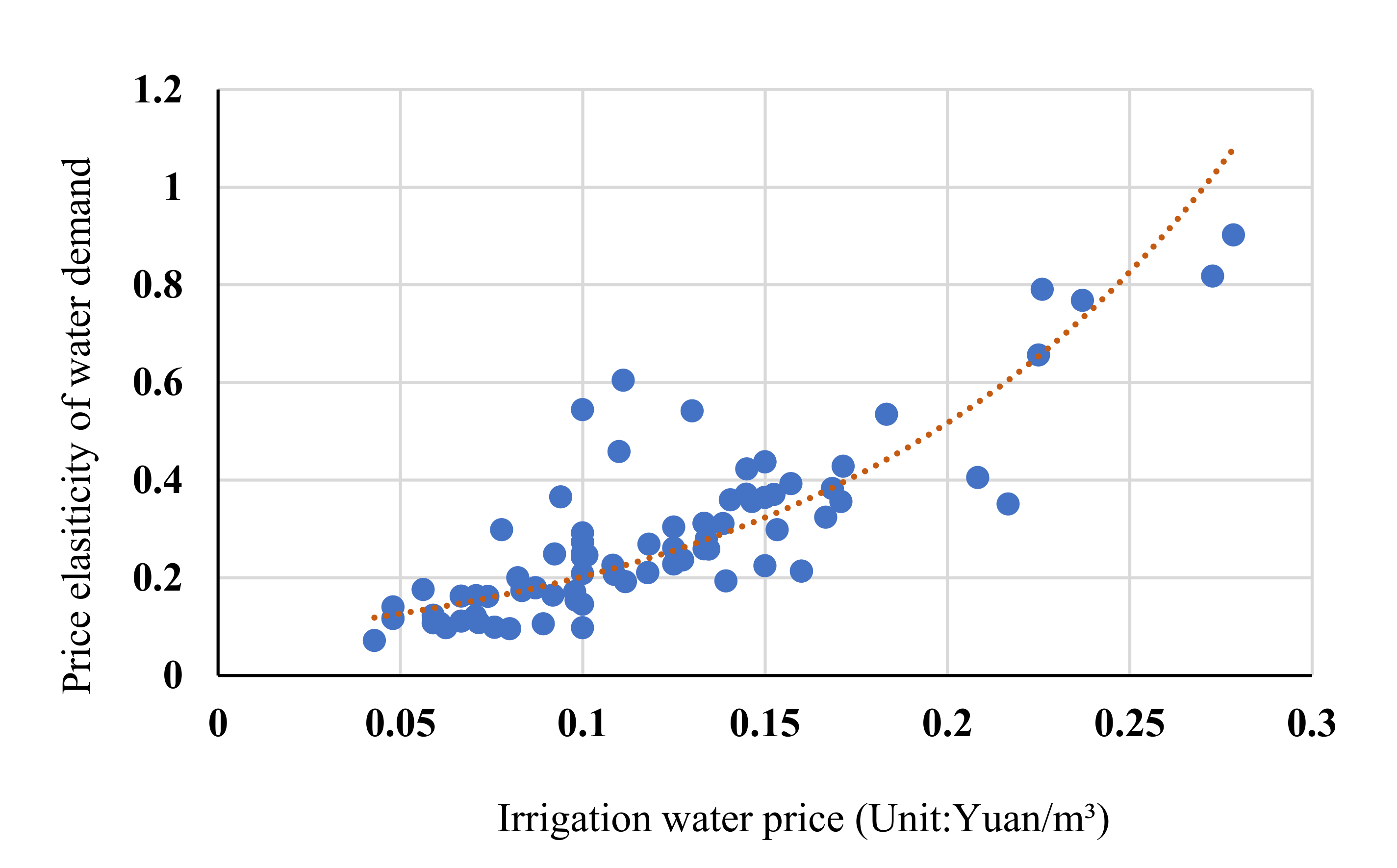
Finally, the inelastic feature is widely considered the main reason for the failure of the price tool in agricultural water management. Previous studies based on different methods, including mathematical programming methods, econometric methods, and experimental research methods, show that irrigation water price elasticity lies between −1.97 and −0.002, with an average of −0.51, revealing that the irrigation water price is inelastic in most areas [8,42]. Other research shows that the price elasticity of agricultural water demand in China is between −0.13 and −0.72, which is much lower than that in developed countries, which ranges between −0.5 and −1.4 [14]. The elastic range determines whether water prices can play a role in regulating irrigation water use. The price elasticity of irrigation water demand is closely related to water prices [43]. Figure 4 shows a logarithmic fitting between the irrigation water price and price elasticity. We can see that price elasticity increases as water price increases. The water demand was found to become elastic at the tipping point of CNY 0.27 per m³, when the price elasticity is close to 1. Therefore, the current low agricultural water price in the HRB is the main impediment to the effective functioning of the price mechanism. The relationship between water price and water demand can also guide future irrigation water price reforms—such as ladder-like water prices and different water price ladders—in reasonably setting prices through the corresponding elasticity of different water prices.

4.2. Estimation of the Elasticity of Substitution of Water and Land

The elasticity of substitution reflects the matching and substitution relationship between different factors. High elasticity between input factors indicates that the substitution between different kinds of resources is relatively flexible. It also indicates that the impact on the economic system is relatively small, since producers can easily adjust various inputs in the production. Water and land resources are the two primary factors for agricultural activities. The elasticity of water and land substitution measures the substitutability between the sown area of irrigated crops and the water used for irrigation [36]. Extensive research has used econometric models to estimate the production function and elasticity of substitution between different input factors such as labour, land, and capital. However, there is a lack of quantitative estimation of the elasticity of substitution between irrigation water and land, which is an important indicator in our WEM.

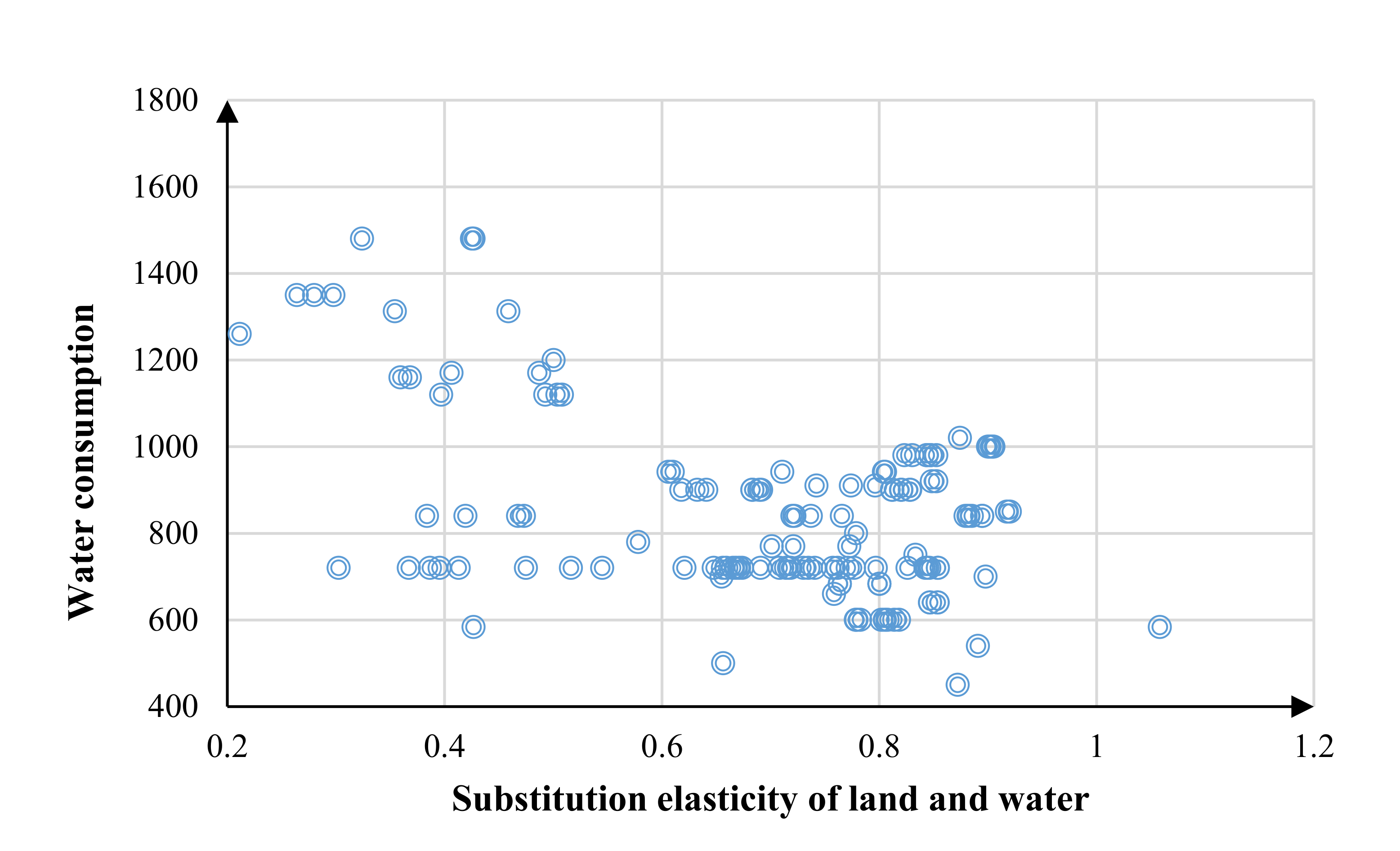
The average elasticity of water and land substitution obtained in this study was 0.43. Previous studies have shown that the substitution elasticity of water and land is generally between 0.04 and 0.7 [33,44]. This indicates that, in our study area, the substitution elasticity of water and land is low in agricultural production. Next, we derived the relationship between irrigation water demand and the substitution elasticity of land and water (Figure 5). The greater the substitution elasticity of land and water, the lower the irrigation water consumption. This explains why the reallocation of water and land will further promote water productivity. Simulations from Sun show that when the substitution elasticity of land and water increases from 0 to 0.7, the water productivity of maize increases from CNY 1.83 per m³ to CNY 2.21 per m³, and the comprehensive water productivity increases from CNY 1.31 per m³ to CNY 1.59 per m³ [44]. The elasticity of water and land substitution rate denotes how water and land will be allocated under different external economic shocks in the WEM.

4.3. Simulation of the Impact of Water Price Change on Economic Development

Irrigation water, as an important primary input for a production process, has the dual attributes of a commodity and a public good; accordingly, a price change of irrigation water will cause a chain reaction in the regional economic system, including aspects such as economic output, employment, income, and the consumption of goods. Therefore, the analysis of the economic impact of water price change on different economic entities is of great significance to water pricing strategies. Taking Gaotai County as an example, a simulation of a water price change from 0.15 to 0.27 was conducted after the calibration of the WEM.

Table 3. Impacts of irrigation water price change on the main economic and production indicators in Gaotai County.

Main Economic Indicators	Change (%)	Main Input Factors	Change (%)
GDP	−1.66	Total water demand	−10.2
Investment	0.07	Surface water demand	−7.11
Consumption of goods	−1.45	Groundwater demand	−16.34
Exports to other regions	−0.66	Other water demand	−5.23
Imports from other regions	−0.11	Nominal wage	−0.073
Consumer purchase index(CPI)	0.008	Price of Capital	0.06
Employment	−0.73	Land rent	−13.10

summarises the changes in the key macroeconomic variables relating to the irrigation water price reform in Gaotai County. It is worth highlighting that the water price increase leads to a 1.66% and 0.73% decline in regional GDP and employment, respectively. The main mechanism behind this is that increments in irrigation water price lead to elevated agricultural costs, which are then transmitted to other industries through the ripple effect of the economy. Further, the increasing cost leads to a 1.45% decrease in the consumer consumption of goods, and exports to other regions diminish by 0.66%. A slight increase in the regional consumer price index (CPI) by 0.008% was also observed in our simulation.

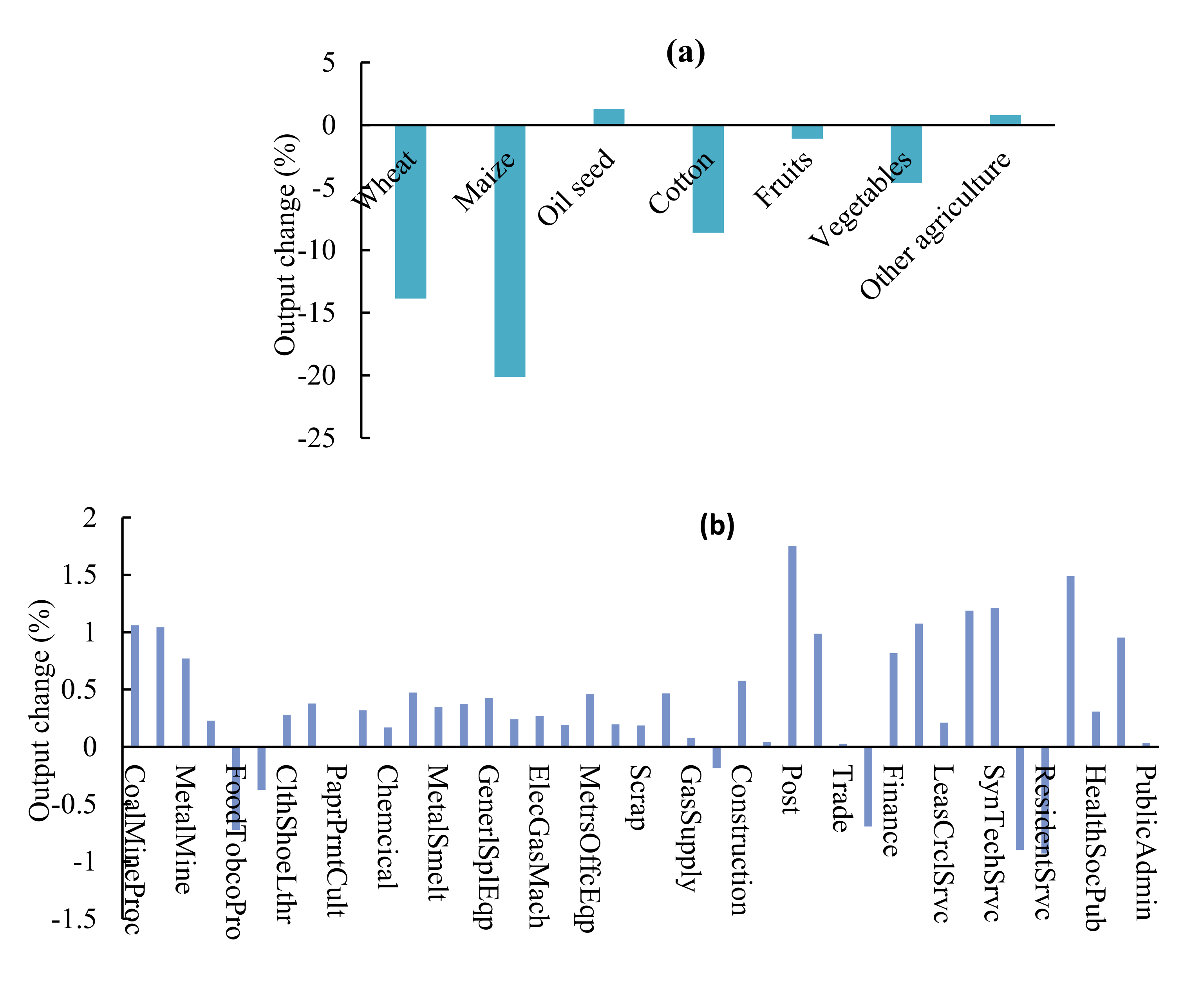
In terms of sectoral outputs, we find that an increase in irrigation water price leads to a reduction in output by major agricultural sectors in the study area. Among these agricultural sectors, the most affected is maize, with the output diminished by 20%, followed by wheat, cotton, and vegetables. The underlying differences in the output change may be attributed to the cost variance of water per unit of output for different crops. The costs of water per unit of output for maize, wheat, and vegetables are relatively high and will be more susceptible to irrigation water price change, which directly leads to contracted output and demand. On the contrary, the output of oilseed and other crops increases slightly. Part of the reason for this is that they need less water during the growing season, and farmers tend to expand their planting area when faced with a higher irrigation cost.

It is worth highlighting that the output of most non-agricultural sectors increases consistently with increasing irrigation price, except for those closely related to the agricultural sectors, including food manufacturing, textiles, residential services, accommodation, and catering, which are downstream sectors of the agricultural sectors (Figure 6). One possible explanation for the reduction in the output of these sectors could be the transmission effects of higher agricultural costs induced by increases in irrigation water prices. However, most non-agricultural sectors will benefit from an increase in irrigation water prices. On the one hand, an increase in irrigation water prices will lead to a demand abatement for land for agriculture; thus, more land will be released from agricultural sectors to non-agricultural sectors. On the other hand, a greater land supply will lead to a decrease in land rent (−13.1%), which will bring a cost advantage for the non-agricultural sectors.

4.4. Impact of Water Price Change on Water Productivity

Focussing on the water demand changes, the results show that the total amount of water used in the economic system decreases significantly, with a 10.2% total decline in water consumption, including a 7.11% and 16.34% decline in surface water and groundwater consumption, respectively. That is, about 0.11 × 10⁹ m³ of surface water and 0.06 × 10⁹ m³ of groundwater can be saved based on the 2012 water-use data. The largest contributor to water saving is the agricultural sector, which contributes 94% of the total water conservation. Water-saving effects vary among different crops. As the main crop in the study area, water consumption by maize decreased by 0.115 × 10⁹ m³. For other crops—wheat, vegetables, and fruits—water consumption decreased by 0.018 × 10⁹ m³, 0.017 × 10⁹ m³, and 0.01 × 10⁹ m³, respectively. Oilseeds and other agricultural sectors are less sensitive to water price changes than the other agricultural sectors. Their output expanded in our simulation. This may imply that the government can change the crop structure to plant more oilseeds and Chinese herbal medicines. In terms of non-agricultural sectors, the total water demand decline is about 0.01 × 10⁹ m³, which mainly comes from the food manufacturing, textiles, residential services, accommodation, and catering sectors. The water demand for other non-agricultural sectors increased slightly.

The change in water demand for surface water and groundwater varies among different industrial sectors. For agricultural sectors, surface water demand decreases more than groundwater demand. This is the opposite of the non-agricultural sectors, where groundwater demand declines more than surface water demand. This is decided by the water-use structure, since agricultural sectors utilise more surface water, whereas non-agricultural sectors use more groundwater. Although groundwater use prevails in non-agricultural sectors, water-intensive agricultural sectors remain the main contributors to groundwater conservation. This is in line with our perception that irrigation water prices will play an important role in regulating agricultural water demand.

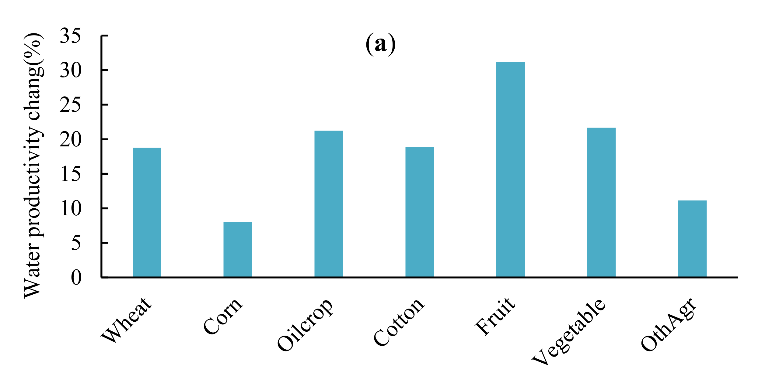
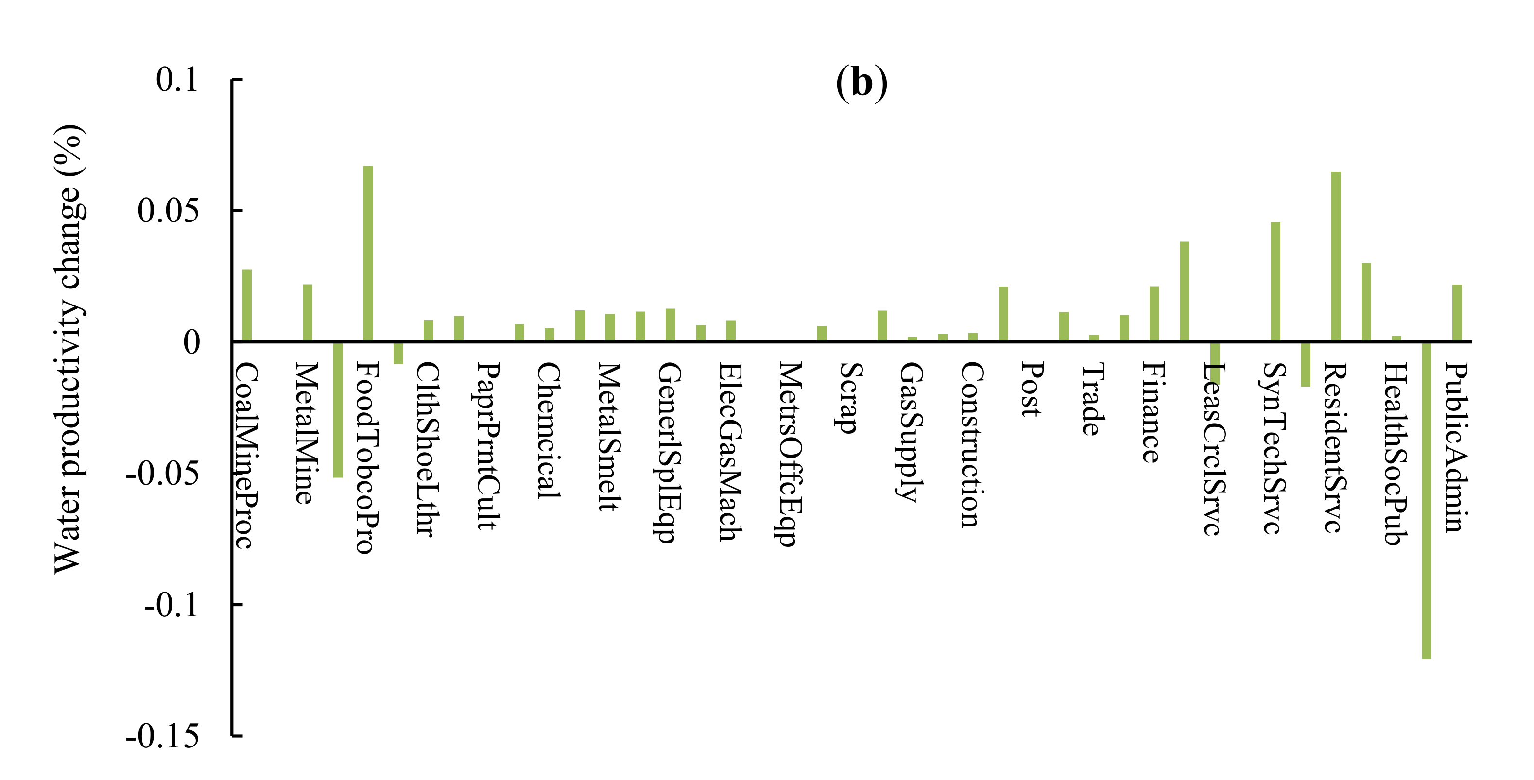
As expected, the water price reform leads to a water productivity improvement in most industries and sectors (Figure 7). Among all sectors, the agricultural sector achieves the greatest improvement in water productivity. However, there is still a gap between different agricultural sectors. For example, water productivity for fruit increases by 30%, changing from CNY 9.7 per m³ to CNY 12 per m³. However, with the largest planting area, water productivity for maize increased by only 6%. There were no significant improvements in water productivity for non-agricultural sectors. Overall, water productivity in the economic system increased by 7.2% and reached CNY 20.5 per m³.

Combined with the above analysis, we find that the water price reform caused the reallocation of water and land resources among industries, which was mainly manifested in the transfer of water and land resources from agricultural to non-agricultural sectors. With an increase in water price, higher production costs will not only lead to the shrinkage of water demand but also of land demand in agricultural sectors. In general, more land will become available for non-agricultural sectors. The greater availability of land resources will eventually induce a fall in land rent, which will further lead to the reallocation of economic factors such as labour and capital among industries. That is to say, a change in water price sparks a chain of events in the economic system. Therefore, it has been proven that water productivity can be improved through these chain effects. It should be noted that raising agricultural water prices will increase the chances of more land being diverted to non-agricultural water use. This shift may cause food shortages and increase food prices. However, the impact is limited, and the benefits are greater in saving water resources and improving water-use efficiency in our case study. On the other hand, we need to be cautious about food security problems when implementing water price reforms in the future. This study is also an attempt to discuss water price problems in the water–land nexus. It highlights the importance of managing water and land resources in an integrated framework to improve water productivity in the future.

In contrast to previous studies focusing on the influence of water price changes on agricultural production, this paper offers an evaluation framework of how to set an appropriate agricultural water price from a water-economic system viewpoint. However, farmers’ responses to water price changes and the welfare loss caused by water price increases need to be considered in future water price reforms. Studies have shown that if prices are beyond farmers’ affordability, they will damage agricultural production [17]. Considering the double-edged sword effect of agricultural water prices, many governments have backtracked from such reforms to ensure food security. For example, water resource fees are not levied, and agricultural water use is charged according to the size of the irrigated area in Japan. In India, the government stipulates that the agricultural water expense must be less than half of the net income of farmers, generally between 5% and 12%, and water is charged based on the irrigation area and crop species. However, the full recovery of agricultural water price costs has been adopted in countries such as France and Australia, where the governmental financial subsidy is relatively low. The optimal prices rely on the objectives of the water agency, and there is no best practice that can be suggested for every country.

Furthermore, considering the increasing water prices, farmers may choose to plant more profitable crops. The economic WP for the main crops in the study area such as maize, wheat, and barley are CNY 4.2 per m³, 3.0 per m³, and 2.8 per m³, respectively. They are far below the WP of fruits, vegetables, and oilseeds. In recent years, economic crops such as oilseeds, vegetables, and Chinese herbal medicines have developed rapidly in the study area, which accounts for almost 80% of the economic crop. This indicates that water pricing policy plays a part in motivating farmers to change their cropping pattern and thus leads to the higher productivity of water. In this research, we could only provide a broad analysis of the crop structure based on the model results, whereas a deeper analysis of cropping patterns is needed in the future involving not only water price but also land-use conditions, farmers’ conceptions, and the market. However, attention should be paid to the impact of water price reform on maize and vegetables, which are competitive agricultural sectors in the study area but also highly dependent on water resources and sensitive to changes in water prices.

4.5. System Sensitivity Analysis

The substitution elasticity of water and land, δlw, in the production function was selected for sensitivity analysis. The system sensitivity analysis (SSA) method was applied, whereby a uniform distribution series obeying [−100%, 100%] is generated with the change of the δlw parameter under the condition that the other parameters remain unchanged. Assuming a 10% increase in water prices, the results are shown in

Table 4. Sensitivity analysis of the model.

Variable	Household Consumption	Investment	Exports	Imports	CPI	RealGDP	Stock of the Capital
Average change (%)	−0.06	−0.08	−0.44	0.11	0.07	−0.20	−0.18
Standard error	0.004	0.003	0.005	0.003	0.001	0.008	0.002

. We can see that the average resident consumption increased by 0.06%, and the standard deviation of each variable index did not exceed 0.008, indicating that the model was stable.

5. Conclusions and Policy Implications

Ensuring high levels of water productivity is of key concern in integrated water resource management in arid and semiarid inland river basins. Thus, this study explores the pricing mechanisms used in regulating the simple and extensive growth mode of water demand and strengthening the connotative development of water saving for water productivity improvement. Previous studies have pointed out that the low elasticity of agricultural water prices is the main reason behind the failure of agricultural water demand management. However, they ignore the fact that water price elasticity is strongly dependent on the price range. This study innovatively examines the relationship between agricultural water price and price elasticity and the elastic range of water prices. The empirical results show that the HRB’s current agricultural water price is inelastic, with a value of −0.26. This is also the case in most developing countries, where water prices are very low and have been subsidized to avoid a negative impact on agricultural production. However, the price elasticity of water demand increases as the price increases. The water demand becomes elastic when the price rises to CNY 0.27 per m³ based on the estimation of the irrigation water demand function. It needs to be mentioned that the optimal price here is based on a simulation. The literature demonstrates that optimal prices rely on the objectives of the water agency and there is no best practice that can be suggested to all countries. However, this paper provides theoretical support and a design reference for the implementation of price means in water resources management, especially in future ladder-like water price reforms; different water price ladders can be reasonably set through the corresponding elasticity of different water prices.

In addition to the above, this study also seeks to better understand the complicated implementation effects of water price reforms on water allocation, water productivity, and economic development. To achieve this, a water-economic model coupled with a water-economic system was built. The simulation results indicated that when raising the water price to the elastic range, the water-saving effects become obvious. The total water consumption in Gaotai County declines by 10.2%, including a 7.11% decline in surface water consumption and a 16.34% decline in groundwater consumption. The overall water productivity increases by 7.2% at the cost of a 1.6% reduction in economic output. It should be noted that the local government should pay attention to and mitigate the impact of the water price reform on maize and vegetables, which are competitive agricultural sectors in the study area, since they are highly dependent on water resources and are sensitive to changes in water prices.

Water price reforms facilitate the reallocation of water and land among industries. The shift in water and land resources from agricultural sectors to non-agricultural sectors is the reform’s main contribution to the improvement of water productivity. On the one hand, due to the increase in agricultural water price, agricultural production shrinks and the demand for water and land decreases. On the other hand, water price increases will accelerate the substitution between water and land in agricultural production, which means less water will be used for the same crop area. Additionally, considering that there are relatively abundant land resources and scarce water resources in the HRB, water and land resources should be managed in an integrated framework.

We conclude that water pricing policies can be expected to help improve water productivity based on the modelling framework this study proposes. However, many unsettled issues still need to be discussed, such as farmers’ responses to water price changes, the welfare loss caused by water price increases, and the guarantee that water resources will flow successfully from agricultural to non-agricultural sectors. In the future, it is imperative to innovate the water resources management system in arid areas by establishing a reasonable water market. This will ensure appropriate price formation mechanisms and promote the buyback of water resources to realise the effective allocation of water resources.

References

- Cheng, G.; Li, X.; Zhao, W.; Xu, Z.; Feng, Q.; Xiao, S.; Xiao, H. Integrated Study of the Water–Ecosystem–Economy in the Heihe River Basin. Natl. Sci. Rev. 2014, 1, 413–428. [Google Scholar] [CrossRef] [Green Version]
- Bakker, K. Water Security: Research Challenges and Opportunities. Science 2012, 337, 914. [Google Scholar] [CrossRef] [PubMed]
- Gleick, P.H. Transitions to Freshwater Sustainability. Proc. Natl. Acad. Sci. USA 2018, 115, 8863–8871. [Google Scholar] [CrossRef] [PubMed] [Green Version]
- Cai, X.; Wallington, K.; Shafiee-Jood, M.; Marston, L. Understanding and Managing the Food-Energy-Water Nexus—Opportunities for Water Resources Research. Adv. Water Resour. 2018, 111, 259–273. [Google Scholar] [CrossRef]
- Chouchane, H.; Hoekstra, A.Y.; Krol, M.S.; Mekonnen, M.M. The Water Footprint of Tunisia from an Economic Perspective. Ecol. Indic. 2015, 52, 311–319. [Google Scholar] [CrossRef] [Green Version]
- Schyns, J.F.; Hoekstra, A.Y.; Booij, M.J.; Hogeboom, R.J.; Mekonnen, M.M. Limits to the World’s Green Water Resources for Food, Feed, Fiber, Timber, and Bioenergy. Proc. Natl. Acad. Sci. USA 2019, 116, 4893–4898. [Google Scholar] [CrossRef] [PubMed] [Green Version]
- Wichelns, D. Water Productivity and Food Security: Considering More Carefully the Farm-Level Perspective. Food Secur. 2015, 7, 247–260. [Google Scholar] [CrossRef]
- Davidson, B.; Hellegers, P. Estimating the Own-Price Elasticity of Demand for Irrigation Water in the Musi Catchment of India. J. Hydrol. 2011, 408, 226–234. [Google Scholar] [CrossRef]
- Speelman, S.; Buysse, J.; Farolfi, S.; Frija, A.; D’Haese, M.; D’Haese, L. Estimating the Impacts of Water Pricing on Smallholder Irrigators in North West Province, South Africa. Agric. Water Manag. 2009, 96, 1560–1566. [Google Scholar] [CrossRef]
- Momeni, M.; Zakeri, Z.; Esfandiari, M.; Behzadian, K.; Zahedi, S.; Razavi, V. Comparative Analysis of Agricultural Water Pricing between Azarbaijan Provinces in Iran and the State of California in the US: A Hydro-Economic Approach. Agric. Water Manag. 2019, 223, 105724. [Google Scholar] [CrossRef]
- Tsur, Y. Optimal Water Pricing: Accounting for Environmental Externalities. Ecol. Econ. 2020, 170, 106429. [Google Scholar] [CrossRef]
- Yudhistira, M.H.; Sastiono, P.; Meliyawati, M. Exploiting Unanticipated Change in Block Rate Pricing for Water Demand Elasticities Estimation: Evidence from Indonesian Suburban Area. Water Resour. Econ. 2020, 32, 100161. [Google Scholar] [CrossRef]
- Schoengold, K.; Sunding, D.L. The Impact of Water Price Uncertainty on the Adoption of Precision Irrigation Systems. Available online: https://onlinelibrary.wiley.com/doi/full/10.1111/agec.12118 (accessed on 7 September 2020).
- Sun, T.; Huang, Q.; Wang, J. Estimation of Irrigation Water Demand and Economic Returns of Water in Zhangye Basin. Available online: https://www.mdpi.com/2073-4441/10/1/19 (accessed on 7 September 2020).
- Zhu, X.; Zhang, G.; Yuan, K.; Ling, H.; Xu, H. Evaluation of Agricultural Water Pricing in an Irrigation District Based on a Bayesian Network. Water 2018, 10, 768. [Google Scholar] [CrossRef] [Green Version]
- Kampas, A.; Petsakos, A.; Rozakis, S. Price Induced Irrigation Water Saving: Unraveling Conflicts and Synergies between European Agricultural and Water Policies for a Greek Water District. Agric. Syst. 2012, 113, 28–38. [Google Scholar] [CrossRef]
- Molle, F.; Venot, J.-P.; Hassan, Y. Irrigation in the Jordan Valley: Are Water Pricing Policies Overly Optimistic? Agric. Water Manag. 2008, 95, 427–438. [Google Scholar] [CrossRef]
- Vasileiou, K.; Mitropoulos, P.; Mitropoulos, I. Optimizing the Performance of Irrigated Agriculture in Eastern England under Different Water Pricing and Regulation Strategies. Nat. Resour. Model. 2014, 27, 128–150. [Google Scholar] [CrossRef]
- Calzadilla, A.; Rehdanz, K.; Tol, R.S.J. Water Scarcity and the Impact of Improved Irrigation Management: A Computable General Equilibrium Analysis. Agric. Econ. 2011, 42, 305–323. [Google Scholar] [CrossRef]
- Reimer, J.J.; Babbar-Sebens, M.; Rivera, S.J. WEST: Water Economy Simulation Tool to Predict Impacts of Economic and Environmental Shocks. Adv. Water Resour. 2020, 142, 103648. [Google Scholar] [CrossRef]
- Sapino, F.; Pérez-Blanco, C.D.; Gutiérrez-Martín, C.; Frontuto, V. An Ensemble Experiment of Mathematical Programming Models to Assess Socio-Economic Effects of Agricultural Water Pricing Reform in the Piedmont Region, Italy. J. Environ. Manag. 2020, 267, 110645. [Google Scholar] [CrossRef]
- Do, P.; Tian, F.; Zhu, T.; Zohidov, B.; Ni, G.; Lu, H.; Liu, H. Exploring Synergies in the Water-Food-Energy Nexus by Using an Integrated Hydro-Economic Optimization Model for the Lancang-Mekong River Basin. Sci. Total Environ. 2020, 728, 137996. [Google Scholar] [CrossRef]
- Gallego-Ayala, J. Selecting Irrigation Water Pricing Alternatives Using a Multi-Methodological Approach. Math. Comput. Model. 2012, 55, 861–883. [Google Scholar] [CrossRef]
- Torres, M.d.O.; Howitt, R.; Rodrigues, L.N. Modeling the Economic Benefits and Distributional Impacts of Supplemental Irrigation. Water Resour. Econ. 2016, 14, 1–12. [Google Scholar] [CrossRef]
- Berglund, E.Z.; Pesantez, J.E.; Rasekh, A.; Shafiee, M.E.; Sela, L.; Haxton, T. Review of Modeling Methodologies for Managing Water Distribution Security. J. Water Resour. Plan. Manag. 2020, 146, 03120001. [Google Scholar] [CrossRef]
- Haavisto, R.; Santos, D.; Perrels, A. Determining Payments for Watershed Services by Hydro-Economic Modeling for Optimal Water Allocation between Agricultural and Municipal Water Use. Water Resour. Econ. 2019, 26, 100127. [Google Scholar] [CrossRef]
- Horridge, M.; Wittwer, G. SinoTERM, a Multi-Regional CGE Model of China. China Econ. Rev. 2008, 19, 628–634. [Google Scholar] [CrossRef]
- Calzadilla, A.; Rehdanz, K.; Tol, R.S.J. The Economic Impact of More Sustainable Water Use in Agriculture: A Computable General Equilibrium Analysis. J. Hydrol. 2010, 384, 292–305. [Google Scholar] [CrossRef]
- Wittwer, G.; Griffith, M. Modelling Drought and Recovery in the Southern Murray-Darling Basin. Aust. J. Agric. Resour. Econ. 2011, 55, 342–359. [Google Scholar] [CrossRef]
- Philip, J.-M.; Sanchez-Choliz, J.; Sarasa, C. Technological Change in Irrigated Agriculture in a Semiarid Region of Spain. Water Resour. Res. 2014, 50, 9221–9235. [Google Scholar] [CrossRef]
- Palatnik, R.R.; Roson, R. Climate Change and Agriculture in Computable General Equilibrium Models: Alternative Modeling Strategies and Data Needs. Clim. Change 2012, 112, 1085–1100. [Google Scholar] [CrossRef]
- Wu, F.; Zhan, J.; Zhang, Q.; Sun, Z.; Wang, Z. Evaluating Impacts of Industrial Transformation on Water Consumption in the Heihe River Basin of Northwest China. Sustainability 2014, 6, 8283. [Google Scholar] [CrossRef] [Green Version]
- Liu, Y.; Hu, X.; Zhang, Q.; Zheng, M. Improving Agricultural Water Use Efficiency: A Quantitative Study of Zhangye City Using the Static CGE Model with a CES Water-Land Resources Account. Sustainability 2017, 9, 308. [Google Scholar] [CrossRef] [Green Version]
- Li, X.; Zhang, Q.; Liu, Y.; Song, J.; Wu, F. Modeling Social–Economic Water Cycling and the Water–Land Nexus: A Framework and an Application. Ecol. Model. 2018, 390, 40–50. [Google Scholar] [CrossRef]
- Shi, M.; Wang, X.; Yang, H.; Wang, T. Pricing or Quota? A Solution to Water Scarcity in Oasis Regions in China: A Case Study in the Heihe River Basin. Sustainability 2014, 6, 7601. [Google Scholar] [CrossRef] [Green Version]
- Kidane, T.T.; Wei, S.; Sibhatu, K.T. Smallholder Farmers’ Willingness to Pay for Irrigation Water: Insights from Eritrea. Agric. Water Manag. 2019, 222, 30–37. [Google Scholar] [CrossRef]
- Wu, F.; Sun, Z.; Wang, F.; Zhang, Q. Identification of the Critical Transmission Sectors and Typology of Industrial Water Use for Supply-Chain Water Pressure Mitigation. Resour. Conserv. Recycl. 2018, 131, 305–312. [Google Scholar] [CrossRef]
- Zhou, Q.; Deng, X.; Wu, F. Impacts of Water Scarcity on Socio-Economic Development: A Case Study of Gaotai County, China. Phys. Chem. Earth Parts ABC 2017, 101, 204–213. [Google Scholar] [CrossRef]
- Kant, S.; Nautiyal, J.C. Production Structure, Factor Substitution, Technical Change, and Total Factor Productivity in the Canadian Logging Industry. Can. J. For. Res. 1997, 27, 701–710. [Google Scholar] [CrossRef]
- Schoengold, K.; Sunding, D.L.; Moreno, G. Price Elasticity Reconsidered: Panel Estimation of an Agricultural Water Demand Function. Water Resour. Res. 2006, 42, W09411. [Google Scholar] [CrossRef] [Green Version]
- Zhou, Q.; Deng, X.; Wu, F.; Li, Z.; Song, W. Participatory Irrigation Management and Irrigation Water Use Efficiency in Maize Production: Evidence from Zhangye City, Northwestern China. Water 2017, 9, 822. [Google Scholar] [CrossRef] [Green Version]
- Sahin, O.; Bertone, E.; Beal, C.D. A Systems Approach for Assessing Water Conservation Potential through Demand-Based Water Tariffs. J. Clean. Prod. 2017, 148, 773–784. [Google Scholar] [CrossRef] [Green Version]
- Liu, X.; Chen, X.; Wang, S. Evaluating and Predicting Shadow Prices of Water Resources in China and Its Nine Major River Basins. Water Resour. Manag. 2009, 23, 1467–1478. [Google Scholar] [CrossRef]
- Sun, Z.; Wu, F.; Shi, C.; Zhan, J. The Impact of Land Use Change on Water Balance in Zhangye City, China. Phys. Chem. Earth Parts ABC 2016, 96, 64–73. [Google Scholar] [CrossRef]
Figure 1.
Heihe River Basin and its location in Northwest China.
Figure 2.
The nested production structure of the WEM.
Figure 3.
The interactive mechanism of water price and water productivity in the WEM.
Figure 4.
Relationship between irrigation water price and the price elasticity of irrigation water demand.
Figure 5.
Relationship between irrigation water and the substitution elasticity of land and water.
Figure 6.
Changes in sectoral output: (a) agricultural sectors; (b) non-agricultural sectors.
Figure 7.
Changes in water productivity: (a) agricultural sectors; (b) non-agricultural sectors.