
Integrating the Strength of Multi-Date Sentinel-1 and -2 Datasets for Detecting Mango (Mangifera indica L.) Orchards in a Semi-Arid Environment in Zimbabwe

 , ,
, ,  , , and
Abstract
:1. Introduction
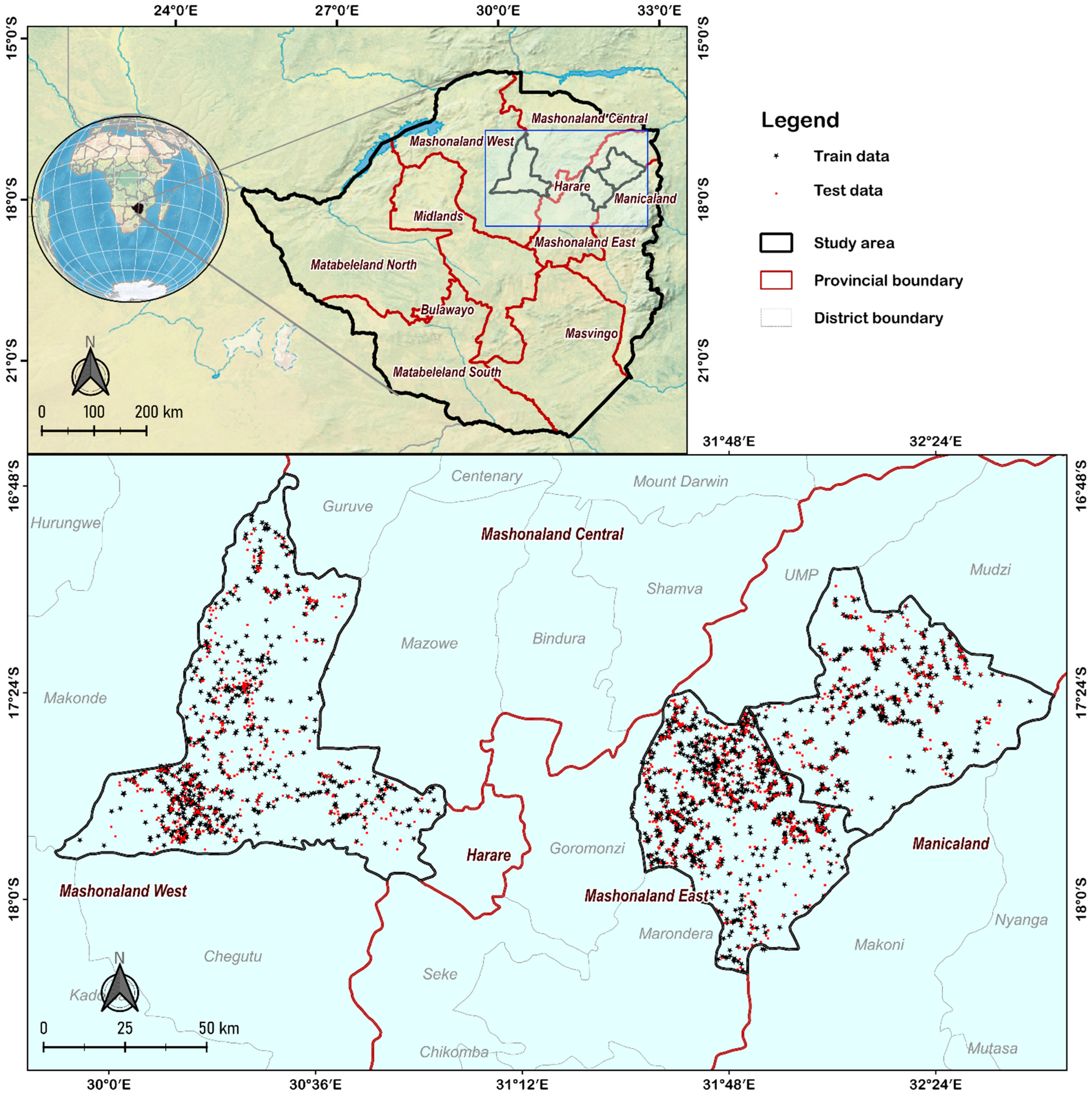
2. Study Area
3. Methodology
3.1. Land Use and Land Cover (LULC) Classes
3.2. Mango and Other Land Use and Land Cover (LULC) Field Data Collection
3.3. Sentinel-2 Image Processing in Google Earth Engine (GEE)
3.4. Sentinel-1 (S1) Image Processing in Google Earth Engine (GEE)
3.5. Variable Selection and Importance
3.6. Mapping of Mango Orchards and Other Land Use and Land Cover (LULC) Classes
3.7. Accuracy Assessment
4. Results
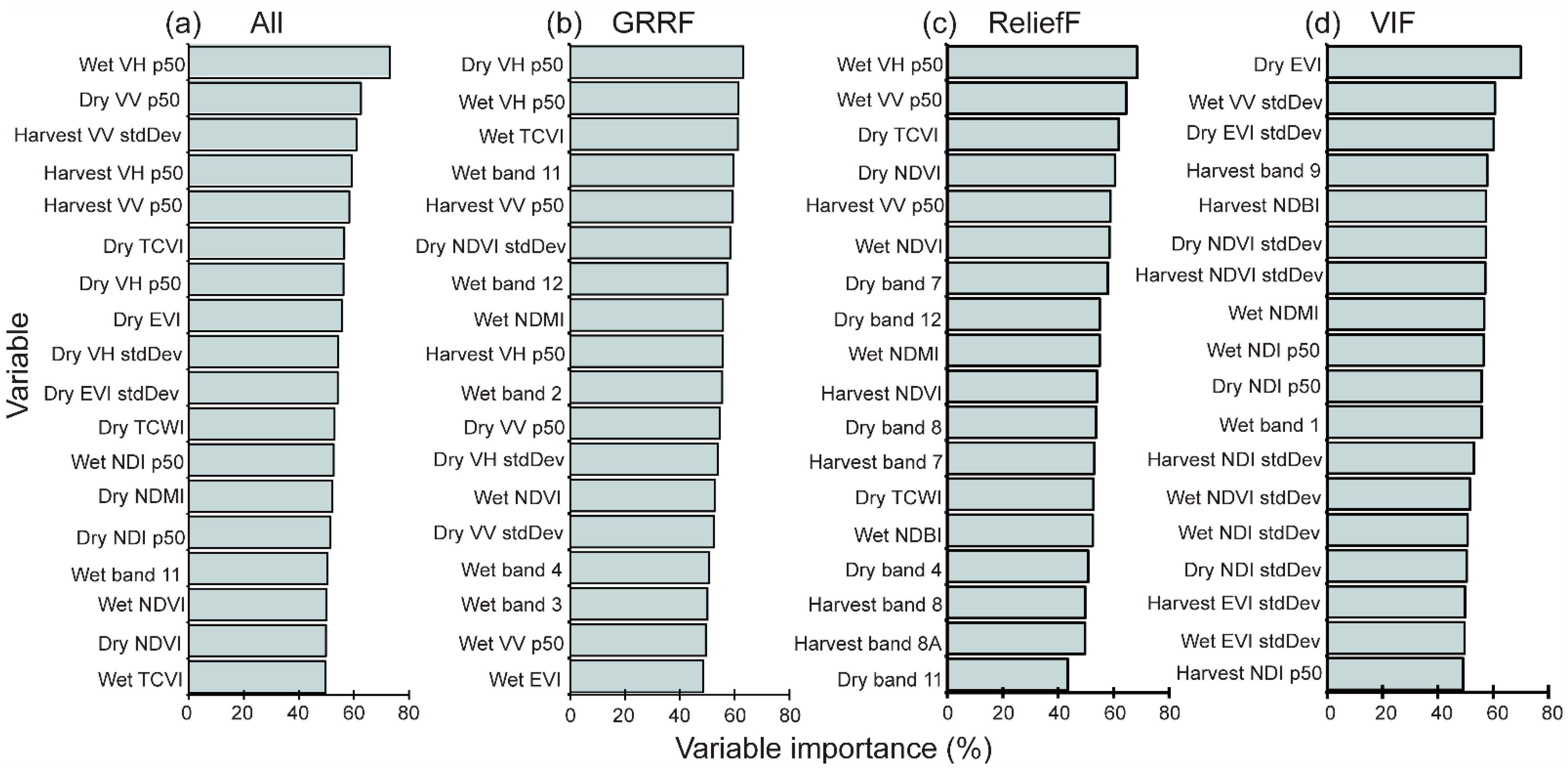
4.1. Variable Selections and Importance
4.2. Mapping Mango and Other Land Use and Land Cover (LULC) Classes
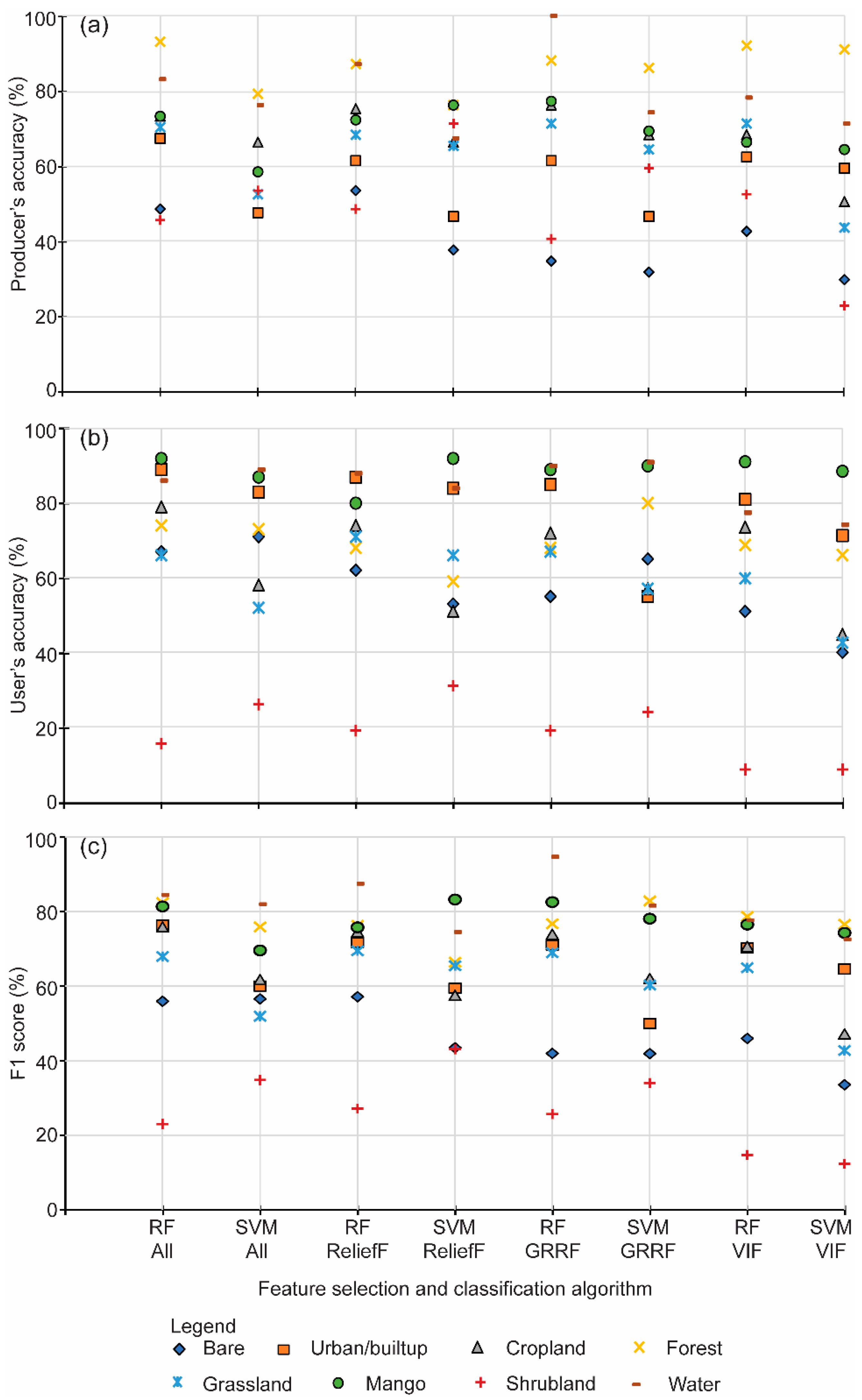
4.3. Analysis of the Classification Accuracies
4.4. Unbiased Area Estimation
5. Discussion
6. Conclusions
Author Contributions
Funding
Data Availability Statement
Acknowledgments
Conflicts of Interest
References
- Luo, H.X.; Dai, S.P.; Li, M.F.; Liu, E.P.; Zheng, Q.; Hu, Y.Y.; Yi, X.P. Comparison of machine learning algorithms for mapping mango plantations based on Gaofen-1 imagery. J. Integr. Agric. 2020, 19, 2815–2828. [Google Scholar] [CrossRef]
- Forkuor, G.; Dimobe, K.; Serme, I.; Tondoh, J.E. Landsat-8 vs. Sentinel-2: Examining the added value of sentinel-2’s red-edge bands to land-use and land-cover mapping in Burkina Faso. GISci. Remote Sens. 2018, 55, 331–354. [Google Scholar] [CrossRef]
- Dobrota, C.T.; Carpa, R.; Butiuc-Keul, A. Analysis of designs used in monitoring crop growth based on remote sensing methods. Turkish J. Agric. For. 2021, 45, 730–742. [Google Scholar] [CrossRef]
- Alkan, A.; Abdullah, M.Ü.; Abdullah, H.O.; Assaf, M.; Zhou, H. A smart agricultural application: Automated detection of diseases in vine leaves using hybrid deep learning. Turkish J. Agric. For. 2021, 45, 717–729. [Google Scholar] [CrossRef]
- Zingore, K.M.; Sithole, G.; Abdel-Rahman, E.M.; Mohamed, S.A.; Ekesi, S.; Tanga, C.M.; Mahmoud, M.E.E. Global risk of invasion by Bactrocera zonata: Implications on horticultural crop production under changing climatic conditions. PLoS ONE 2020, 15, e0243047. [Google Scholar] [CrossRef]
- FAO; IFAD; UNICEF; WFP; WHO. The State of Food Security and Nutrition in the World 2021. In Transforming Food Systems for Food Security, Improved Nutrition and Affordable Healthy Diets for All; FAO: Rome, Italy, 2021; ISBN 9789251329016. [Google Scholar]
- FAO. How to Feed the World in 2050. Insights from an Expert Meet; FAO: Rome, Italy, 2009; pp. 1–35. [Google Scholar] [CrossRef]
- FAO. Fruit and Vegetables—Your Dietary Essentials; FAO: Rome, Italy, 2020; ISBN 9789251337097. [Google Scholar]
- Durán Zuazo, V.H.; Rodríguez Pleguezuelo, C.R.; Gálvez Ruiz, B.; Gutiérrez Gordillo, S.; García-Tejero, I.F. Water use and fruit yield of mango (Mangifera indica L.) grown in a subtropical Mediterranean climate. Int. J. Fruit Sci. 2019, 19, 136–150. [Google Scholar] [CrossRef]
- FAOSTAT Crops and Livestock Products: Mangoes, Mangosteens and Guavas. Available online: https://www.fao.org/faostat/en/#data/QCL (accessed on 3 February 2022).
- Mujuka, E.; Mburu, J.; Ogutu, A.; Ambuko, J.; Magambo, G. Consumer awareness and willingness to pay for naturally preserved solar-dried mangoes: Evidence from Nairobi, Kenya. J. Agric. Food Res. 2021, 5, 100188. [Google Scholar] [CrossRef]
- Mithöfer, D. Economics of Indigenous Fruit Tree Crops in Zimbabwe. Ph.D. thesis, University of Hannover, Hannover, Germany, 2004. [Google Scholar]
- Ekesi, S.; Mohamed, S.A.; Meyer, M. Fruit Fly Research and Development in Africa—Towards A Sustainable Management Strategy to Improve Horticulture; Springer: Cham, Switzerland, 2016; ISBN 9783319432243. [Google Scholar]
- Ekesi, S.; Billah, M.K.; Nderitu, P.W.; Lux, S.A.; Rwomushana, I. Evidence for competitive displacement of Ceratitis cosyra by the invasive fruit fly Bactrocera invadens (Diptera: Tephritidae) on mango and mechanisms contributing to the displacement. J. Econ. Entomol. 2009, 102, 981–991. [Google Scholar] [CrossRef]
- Nankinga, C.M.; Isabirye, B.E.; Muyinza, H.; Rwomushana, I.; Stevenson, P.C.; Mayamba, A. Fruit fly infestation in mango: A threat to the Horticultural sector in Uganda. Uganda J. Agric. Sci. 2014, 15, 1–14. [Google Scholar]
- Dobrini, D.; Gašparovi, M.; Medak, D. Sentinel-1 and 2 Time-Series for vegetation mapping using random forest classification: A Case Study of Northern Croatia. Remote Sens. 2021, 13, 2321. [Google Scholar] [CrossRef]
- Campbell, J.; Wynne, R. Introduction to Remote Sensing, 5th ed.; Guiford Press: New York, NY, USA, 2007; Volume 136, ISBN 9781609181765. [Google Scholar]
- Immitzer, M.; Vuolo, F.; Atzberger, C. First experience with Sentinel-2 data for crop and tree species classifications in central Europe. Remote Sens. 2016, 8, 166. [Google Scholar] [CrossRef]
- Ramoelo, A.; Cho, M.; Mathieu, R.; Skidmore, A.K. Potential of Sentinel-2 spectral configuration to assess rangeland quality. J. Appl. Remote Sens. 2015, 9, 094096. [Google Scholar] [CrossRef] [Green Version]
- Chemura, A.; Mutanga, O.; Odindi, J.; Kutywayo, D. Mapping spatial variability of foliar nitrogen in coffee (Coffea arabica L.) plantations with multispectral Sentinel-2 MSI data. ISPRS J. Photogramm. Remote Sens. 2018, 138, 1–11. [Google Scholar] [CrossRef]
- Belgiu, M.; Csillik, O. Sentinel-2 cropland mapping using pixel-based and object-based time-weighted dynamic time warping analysis. Remote Sens. Environ. 2018, 204, 509–523. [Google Scholar] [CrossRef]
- Mudereri, B.T.; Chitata, T.; Mukanga, C.; Mupfiga, T.; Gwatirisa, C.; Dube, T. Can biophysical parameters derived from Sentinel-2 space-borne sensor improve land cover characterisation in semi-arid regions? Geocarto Int. 2021, 36, 2204–2223. [Google Scholar] [CrossRef]
- Schulz, D.; Yin, H.; Tischbein, B.; Verleysdonk, S.; Adamou, R.; Kumar, N. Land use mapping using Sentinel-1 and Sentinel-2 time series in a heterogeneous landscape in Niger, Sahel. ISPRS J. Photogramm. Remote Sens. 2021, 178, 97–111. [Google Scholar] [CrossRef]
- ESA Sentinel-2 Products Specification. Available online: https://sentinel.esa.int/web/sentinel/missions/sentinel-2/data-products (accessed on 30 April 2019).
- Cheng, K.; Wang, J. Forest-type classification using time-weighted dynamic timewarping analysis in mountain areas: A case study in southern China. Forests 2019, 10, 1040. [Google Scholar] [CrossRef] [Green Version]
- Shoko, C.; Mutanga, O. Examining the strength of the newly-launched Sentinel 2 MSI sensor in detecting and discriminating subtle differences between C3 and C4 grass species. ISPRS J. Photogramm. Remote Sens. 2017, 129, 32–40. [Google Scholar] [CrossRef]
- West, H.; Quinn, N.; Horswell, M. Remote sensing for drought monitoring & impact assessment: Progress, past challenges and future opportunities. Remote Sens. Environ. 2019, 232, 111291. [Google Scholar] [CrossRef]
- Pandey, A.C.; Kaushik, K.; Parida, B.R. Google Earth Engine for large-scale flood mapping using SAR data and impact assessment on agriculture and population of Ganga-Brahmaputra basin. Sustainability 2022, 14, 4210. [Google Scholar] [CrossRef]
- Aduvukha, G.R.; Abdel-rahman, E.M.; Sichangi, A.W.; Makokha, G.O.; Landmann, T.; Mudereri, B.T.; Tonnang, H.E.Z.; Dubois, T. Cropping pattern mapping in an agro-natural heterogeneous landscape using Sentinel-2 and Sentinel-1 satellite datasets. Agriculture 2021, 11, 530. [Google Scholar] [CrossRef]
- Gxokwe, S.; Dube, T.; Mazvimavi, D. Leveraging Google Earth Engine platform to characterize and map small seasonal wetlands in the semi-arid environments of South Africa. Sci. Total Environ. 2021, 803, 150139. [Google Scholar] [CrossRef] [PubMed]
- Nhu, V.H.; Mohammadi, A.; Shahabi, H.; Ahmad, B.B.; Al-Ansari, N.; Shirzadi, A.; Geertsema, M.; Kress, V.R.; Karimzadeh, S.; Kamran, K.V.; et al. Landslide detection and susceptibility modeling on cameron highlands (Malaysia): A comparison between random forest, logistic regression and logistic model tree algorithms. Forests 2020, 11, 830. [Google Scholar] [CrossRef]
- Ahmad, A.; Gilani, H.; Ahmad, S.R. Forest aboveground biomass estimation and mapping through high-resolution optical satellite imagery—A literature review. Forests 2021, 12, 914. [Google Scholar] [CrossRef]
- Georganos, S.; Grippa, T.; Vanhuysse, S.; Lennert, M.; Shimoni, M.; Kalogirou, S.; Wolff, E. Less is more: Optimizing classification performance through feature selection in a very-high-resolution remote sensing object-based urban application. GIScience Remote Sens. 2018, 55, 221–242. [Google Scholar] [CrossRef]
- Urbanowicz, R.J.; Meeker, M.; La Cava, W.; Olson, R.S.; Moore, J.H. Relief-based feature selection: Introduction and review. J. Biomed. Inform. 2018, 85, 189–203. [Google Scholar] [CrossRef]
- Urszula, S.; Zielosko, B.; Jain, L.C. Advances in Feature Selection for Data and Pattern Recognition; Springer: Cham, Switzerland, 2018; Volume 138, ISBN 9783319136592. [Google Scholar]
- Chandrashekar, G.; Sahin, F. A survey on feature selection methods. Comput. Electr. Eng. 2014, 40, 16–28. [Google Scholar] [CrossRef]
- Mtengwana, B.; Dube, T.; Mudereri, B.T.; Shoko, C. Modeling the geographic spread and proliferation of invasive alien plants (IAPs) into new ecosystems using multi-source data and multiple predictive models in the Heuningnes catchment, South Africa. GIScience Remote Sens. 2021, 58, 483–500. [Google Scholar] [CrossRef]
- De Leeuw, J. Journal of statistical software. Wiley Interdiscip. Rev. Comput. Stat. 2009, 1, 128–129. [Google Scholar] [CrossRef] [Green Version]
- Breiman, L. Random forests. Mach. Learn. 2001, 45, 5–32. [Google Scholar] [CrossRef] [Green Version]
- Deng, H.; Runger, G. Gene selection with guided regularized random forest. Pattern Recognit. 2013, 46, 3483–3489. [Google Scholar] [CrossRef] [Green Version]
- Vapnik, V. Estimation of Dependences Based on Empirical Data. Nauk. Moscow Transl. 1979, 27, 5165–5184. [Google Scholar]
- Muthoni, F.K.; Odongo, V.O.; Ochieng, J.; Mugalavai, E.M.; Mourice, S.K.; Hoesche-Zeledon, I.; Mwila, M.; Bekunda, M. Long-term spatial-temporal trends and variability of rainfall over Eastern and Southern Africa. Theor. Appl. Climatol. 2019, 137, 1869–1882. [Google Scholar] [CrossRef] [Green Version]
- Mugandani, R.; Wuta, M.; Makarau, A.; Chipindu, B. RE-Classification of Agro-ecological regions of Zimbabwe in conformity with climate variability and change. Afr. Crop Sci. J. 2012, 20, 361–369. [Google Scholar]
- Kuri, F.; Murwira, A.; Murwira, K.S.; Masocha, M. Accounting for phenology in maize yield prediction using remotely sensed dry dekads. Geocarto Int. 2018, 33, 723–736. [Google Scholar] [CrossRef]
- Ouma, T.; Kavoo, A.; Wainaina, C.; Ogunya, B.; Karanja, M.; Kumar, P.L.; Shah, T. Open data kit (ODK) in crop farming: Mobile data collection for seed yam tracking in Ibadan, Nigeria. J. Crop Improv. 2019, 33, 605–619. [Google Scholar] [CrossRef]
- Tonnang, H.E.Z.; Balemi, T.; Masuki, K.F.; Mohammed, I.; Adewopo, J.; Adnan, A.A.; Mudereri, B.T.; Vanlauwe, B.; Craufurd, P. Rapid acquisition, management, and analysis of spatial Maize (Zea mays L.) phenological data—Towards ‘Big Data’ for agronomy transformation in Africa. Agronomy 2020, 10, 1363. [Google Scholar] [CrossRef]
- R Core. Team R: A Language and Environment for Statistical Computing; R Foundation for Statistical Computing: Vienna, Austria; Available online: https://www.R-project.org/ (accessed on 18 November 2021).
- Kuhn, M. Package ‘caret’ R topics documented: CRAN Repos. 2020. Available online: https://CRAN.R-project.org/package=caret (accessed on 18 November 2021).
- Maskell, G.; Chemura, A.; Nguyen, H.; Gornott, C.; Mondal, P. Integration of Sentinel optical and radar data for mapping smallholder coffee production systems in Vietnam. Remote Sens. Environ. 2021, 266, 112709. [Google Scholar] [CrossRef]
- Gorelick, N.; Hancher, M.; Dixon, M.; Ilyushchenko, S.; Thau, D.; Moore, R. Google Earth Engine: Planetary-scale geospatial analysis for everyone. Remote Sens. Environ. 2017, 202, 18–27. [Google Scholar] [CrossRef]
- WFP. Seasonal Overview and Regional Southern African Vulnerability Analysis (2020/2021); WFP: Johannesburg, South Africa, 2021. [Google Scholar]
- Bey, A.; Jetimane, J.; Lisboa, S.N.; Ribeiro, N.; Sitoe, A.; Meyfroidt, P. Mapping smallholder and large-scale cropland dynamics with a flexible classification system and pixel-based composites in an emerging frontier of Mozambique. Remote Sens. Environ. 2020, 239, 111611. [Google Scholar] [CrossRef]
- Mudereri, B.T.; Abdel-Rahman, E.M.; Dube, T.; Niassy, S.; Khan, Z.; Tonnang, H.E.Z.; Landmann, T. A two-step approach for detecting Striga in a complex agroecological system using Sentinel-2 data. Sci. Total Environ. 2021, 762, 143151. [Google Scholar] [CrossRef] [PubMed]
- Henrich, V.; Krauss, G.; Gotze, C.; Sandow, C.; IDB. Entwicklung einer Datenbank für Fernerkundungsindizes. Available online: www.indexdatabase.de (accessed on 18 November 2021).
- Xue, J.; Su, B. Significant remote sensing vegetation indices: A review of developments and applications. J. Sens. 2017, 2017, 1353691. [Google Scholar] [CrossRef] [Green Version]
- Chemura, A.; Mutanga, O.; Dube, T. Separability of coffee leaf rust infection levels with machine learning methods at Sentinel-2 MSI spectral resolutions. Precis. Agric. 2017, 18, 859–881. [Google Scholar] [CrossRef]
- Camargo, F.F.; Sano, E.E.; Almeida, C.M.; Mura, J.C.; Almeida, T. A comparative assessment of machine-learning techniques for land use and land cover classification of the Brazilian tropical savanna using ALOS-2/PALSAR-2 polarimetric images. Remote Sens. 2019, 11, 1600. [Google Scholar] [CrossRef] [Green Version]
- Odipo, V.O.; Nickless, A.; Berger, C.; Baade, J.; Urbazaev, M.; Walther, C.; Schmullius, C. Assessment of aboveground woody biomass dynamics using terrestrial laser scanner and L-band ALOS PALSAR data in South African Savanna. Forests 2016, 7, 294. [Google Scholar] [CrossRef] [Green Version]
- Brown, C.; Daniels, A.; Boyd, D.S.; Sowter, A.; Foody, G.; Kara, S. Investigating the potential of radar interferometry for monitoring rural artisanal cobalt mines in the democratic republic of the congo. Sustainability 2020, 12, 9834. [Google Scholar] [CrossRef]
- Patel, P.; Srivastava, H.S.; Panigrahy, S.; Parihar, J.S. Comparative evaluation of the sensitivity of multi-polarized multi-frequency SAR backscatter to plant density. Int. J. Remote Sens. 2006, 27, 293–305. [Google Scholar] [CrossRef]
- Jin, Z.; Azzari, G.; You, C.; Di Tommaso, S.; Aston, S.; Burke, M.; Lobell, D.B. Smallholder maize area and yield mapping at national scales with Google Earth Engine. Remote Sens. Environ. 2019, 228, 115–128. [Google Scholar] [CrossRef]
- ESA Sentinel Online: User Guides Sentinel-1 SAR Product Types and Processing Levels. Available online: https://sentinels.copernicus.eu/web/sentinel/user-guides/sentinel-1-sar/product-types-processing-levels/level-1 (accessed on 15 November 2021).
- Lee, J.S.; Wen, J.H.; Ainsworth, T.L.; Chen, K.S.; Chen, A.J. Improved sigma filter for speckle filtering of SAR imagery. IEEE Trans. Geosci. Remote Sens. 2009, 47, 202–213. [Google Scholar] [CrossRef]
- Izquierdo-Verdiguier, E.; Zurita-Milla, R. An evaluation of guided regularized random forest for classification and regression tasks in remote sensing. Int. J. Appl. Earth Obs. Geoinf. 2020, 88, 102051. [Google Scholar] [CrossRef]
- Mureriwa, N.; Adam, E.; Sahu, A.; Tesfamichael, S. Examining the spectral separability of Prosopis glandulosa from co-existent species using field spectral measurement and guided regularized random forest. Remote Sens. 2016, 8, 144. [Google Scholar] [CrossRef] [Green Version]
- Naimi, B.; Hamm, N.A.S.; Groen, T.A.; Skidmore, A.K.; Toxopeus, A.G. Where is positional uncertainty a problem for species distribution modelling? Ecography 2014, 37, 191–203. [Google Scholar] [CrossRef]
- Romanski, P.; Kotthoff, L.; Schratz, P. FSelector: Selecting Attributes. R package version 0.33. 2021. Available online: https://CRAN.R-project.org/package=FSelector (accessed on 18 November 2021).
- Mushore, T.D.; Mutanga, O.; Odindi, J.; Dube, T. Linking major shifts in land surface temperatures to long term land use and land cover changes: A case of Harare, Zimbabwe. Urban Clim. 2017, 20, 120–134. [Google Scholar] [CrossRef]
- Olofsson, P.; Foody, G.M.; Stehman, S.V.; Woodcock, C.E. Making better use of accuracy data in land change studies: Estimating accuracy and area and quantifying uncertainty using stratified estimation. Remote Sens. Environ. 2013, 129, 122–131. [Google Scholar] [CrossRef]
- Card, D.H. Using known map category marginal frequencies to improve estimates of thematic map accuracy. Photogramm. Eng. Remote Sens. 1982, 48, 431–439. [Google Scholar]
- Stehman, S.V.; Mousoupetros, J.; McRoberts, R.E.; Næsset, E.; Pengra, B.W.; Xing, D.; Horton, J.A. Incorporating interpreter variability into estimation of the total variance of land cover area estimates under simple random sampling. Remote Sens. Environ. 2022, 269, 112806. [Google Scholar] [CrossRef]
- Shibia, M.G.; Röder, A.; Fava, F.P.; Stellmes, M.; Hill, J. Integrating satellite images and topographic data for mapping seasonal grazing management units in pastoral landscapes of eastern Africa. J. Arid Environ. 2022, 197. [Google Scholar] [CrossRef]
- Mudereri, B.T.; Mukanga, C.; Mupfiga, E.T.; Gwatirisa, C.; Kimathi, E.; Chitata, T. Analysis of potentially suitable habitat within migration connections of an intra-African migrant-the Blue Swallow (Hirundo atrocaerulea). Ecol. Inform. 2020, 57, 101082. [Google Scholar] [CrossRef]
- McNemar, Q. Note on the sampling error of the difference between correlated proportions or percentages. Psychometrika 1947, 12, 153–157. [Google Scholar] [CrossRef]
- Zvobgo, L.; Tsoka, J. Deforestation rate and causes in Upper Manyame Sub-Catchment, Zimbabwe: Implications on achieving national climate change mitigation targets. Trees For. People 2021, 5, 100090. [Google Scholar] [CrossRef]
- Csillik, O.; Belgiu, M. Cropland mapping from Sentinel-2 time series data using object-based image analysis. In Proceedings of the 20th AGILE International Conference on Geographic Information Science Societal Geo-Innovation Celebrating, Wageningen, The Netherlands, 9–12 May 2017. [Google Scholar]
- CABI Mango: Mangifera Indica. Available online: https://www.cabi.org/isc/datasheet/34505 (accessed on 7 February 2022).
- Holden, P.B.; Rebelo, A.J.; New, M.G. Mapping invasive alien trees in water towers: A combined approach using satellite data fusion, drone technology and expert engagement. Remote Sens. Appl. Soc. Environ. 2021, 21, 100448. [Google Scholar] [CrossRef]
- Royimani, L.; Mutanga, O.; Odindi, J.; Zolo, K.S.; Sibanda, M.; Dube, T. Distribution of Parthenium hysterophoru L. with variation in rainfall using multi-year SPOT data and random forest classification. Remote Sens. Appl. Soc. Environ. 2019, 13, 215–223. [Google Scholar] [CrossRef]
- Makaya, N.P.; Mutanga, O.; Kiala, Z.; Dube, T.; Seutloali, K.E. Assessing the potential of Sentinel-2 MSI sensor in detecting and mapping the spatial distribution of gullies in a communal grazing landscape. Phys. Chem. Earth 2019, 112, 66–74. [Google Scholar] [CrossRef]
- Noi, P.T.; Kappas, M. Comparison of random forest, k-nearest neighbor, and support vector machine classifiers for land cover classification using sentinel-2 imagery. Sensors 2018, 18, 18. [Google Scholar] [CrossRef] [Green Version]
- Jönsson, P.; Eklundh, L. TIMESAT—A program for analyzing time-series of satellite sensor data. Comput. Geosci. 2004, 30, 833–845. [Google Scholar] [CrossRef] [Green Version]


| LULC Class | Class Number | Training Data (60%) | Test Data (40%) | Total |
|---|---|---|---|---|
| Mango | 1 | 644 | 428 | 1072 |
| Built-up | 2 | 227 | 150 | 377 |
| Cropland | 3 | 263 | 175 | 438 |
| Forest | 4 | 173 | 114 | 287 |
| Grassland | 5 | 185 | 122 | 307 |
| Bare soil | 6 | 83 | 55 | 138 |
| Shrubland | 7 | 88 | 58 | 146 |
| Water | 8 | 143 | 95 | 238 |
| Total | 1806 | 1197 | 3003 |
| Band Number/Index | Description | Central Wavelength (nm) | Width | Original Spatial Resolution (m) |
|---|---|---|---|---|
| B1 | Coastal aerosol | 443 | 20 | 60 |
| B2 | Blue | 490 | 65 | 10 |
| B3 | Green | 560 | 35 | 10 |
| B4 | Red | 665 | 30 | 10 |
| B5 | Red-edge (RE5) | 705 | 15 | 20 |
| B6 | Red-edge (RE6) | 740 | 15 | 20 |
| B7 | Red-edge (RE7) | 783 | 20 | 20 |
| B8 | Near infrared | 842 | 115 | 10 |
| B8A | Rededge NIR | 865 | 20 | 20 |
| B9 | Water vapor | 945 | 20 | 60 |
| B11 | Short wave infrared | 1610 | 90 | 20 |
| B12 | Short wave infrared | 2190 | 180 | 20 |
| EVI | Enhanced vegetation index | NA 1 | NA | NA |
| EVI_stdDev 2 | EVI standard deviation | NA | NA | NA |
| NDBI | Normalized difference build-up index | NA | NA | NA |
| NDMI | Normalized difference moisture index | NA | NA | NA |
| NDVI | Normalized difference vegetation index | NA | NA | NA |
| NDVI_stdDev | NDVI standard deviation | NA | NA | NA |
| TCBI | Tasseled cap brightness index | NA | NA | NA |
| TCVI | Tasseled cap greenness index | NA | NA | NA |
| TCWI | Tasseled cap wetness index | NA | NA | NA |
| Band or Index | Wavelength or Formula |
|---|---|
| VV_p50 | Vertically polarized backscatter with refined lee filter (seasonal mean) |
| VH_p50 | Horizontally polarized backscatter with refined lee filter (seasonal mean) |
| VV_stdDev 3 | The seasonal standard deviation of VV |
| VH_stdDev | The seasonal standard deviation of VH |
| NDI_VV | (VV − VH)/(VV + VH) |
| NDI_VH | (VH − VV)/(VH + VV) |
| Sensor | Once | Twice | Thrice | Four Times |
|---|---|---|---|---|
| Sentinel-1 | 13 | 7 | 2 | 0 |
| Sentinel-2 | 21 | 9 | 0 | 0 |
| Total | 34 | 16 | 2 | 0 |
| Classifier | RF | SVM | ||||
|---|---|---|---|---|---|---|
| Variable Selection Method | Training Overall Accuracy (%) | Test Overall Accuracy (%) | Kappa | Training Overall Accuracy (%) | Test Overall Accuracy (%) | Kappa |
| ‘All’ | 100 | 80 | 0.7 | 89 | 74 | 0.6 |
| ReliefF | 100 | 78 | 0.7 | 76 | 74 | 0.6 |
| GRRF | 100 | 77 | 0.7 | 77 | 72 | 0.6 |
| VIF | 100 | 75 | 0.6 | 68 | 66 | 0.5 |
| RF ‘ALL’ | SVM ‘ALL’ | RF ReliefF | SVM ReliefF | RF GRRF | SVM GRRF | RF VIF | SVM VIF | |
|---|---|---|---|---|---|---|---|---|
| RF ‘ALL’ | – 4 | – | – | – | – | – | – | – |
| SVM ‘ALL’ | 0.6344 | – | – | – | – | – | – | – |
| RF ReliefF | 0.6738 | 0.6409 | – | – | – | – | – | – |
| SVM ReliefF | 0.6321 | 0.6008 | 0.6238 | – | – | – | – | – |
| RF GRRF | 0.6602 | 0.6279 | 0.6517 | 0.6265 | – | – | – | – |
| SVM GRRF | 0.6174 | 0.5867 | 0.6093 | 0.5854 | 0.6013 | – | – | – |
| RF VIF | 0.6436 | 0.6118 | 0.6352 | 0.6105 | 0.6269 | 0.6023 | – | – |
| SVM VIF | 0.5591 | 0.531 | 0.5517 | 0.5299 | 0.5444 | 0.5226 | 0.5357 | – |
| Class | Unbiased Area Estimate (ha) | Area (%) | 95% CI of the Unbiased Area Estimate (ha) |
|---|---|---|---|
| Mango | 292,232 | 18 | ±29,358 |
| Built-up | 151,147 | 9 | ±20,141 |
| Cropland | 529,021 | 33 | ±37,160 |
| Forest | 271,183 | 17 | ±34,127 |
| Grassland | 256,377 | 16 | ±31,994 |
| Bare soil | 26,199 | 2 | ±9506 |
| Shrubland | 54,771 | 3 | ±20,841 |
| Water | 28,797 | 2 | ±5606 |
| Total | 1,609,726 | 100 |
Publisher’s Note: MDPI stays neutral with regard to jurisdictional claims in published maps and institutional affiliations. |
© 2022 by the authors. Licensee MDPI, Basel, Switzerland. This article is an open access article distributed under the terms and conditions of the Creative Commons Attribution (CC BY) license (https://creativecommons.org/licenses/by/4.0/).
Share and Cite
Mudereri, B.T.; Abdel-Rahman, E.M.; Ndlela, S.; Makumbe, L.D.M.; Nyanga, C.C.; Tonnang, H.E.Z.; Mohamed, S.A. Integrating the Strength of Multi-Date Sentinel-1 and -2 Datasets for Detecting Mango (Mangifera indica L.) Orchards in a Semi-Arid Environment in Zimbabwe. Sustainability 2022, 14, 5741. https://doi.org/10.3390/su14105741
Mudereri BT, Abdel-Rahman EM, Ndlela S, Makumbe LDM, Nyanga CC, Tonnang HEZ, Mohamed SA. Integrating the Strength of Multi-Date Sentinel-1 and -2 Datasets for Detecting Mango (Mangifera indica L.) Orchards in a Semi-Arid Environment in Zimbabwe. Sustainability. 2022; 14(10):5741. https://doi.org/10.3390/su14105741
Chicago/Turabian StyleMudereri, Bester Tawona, Elfatih M. Abdel-Rahman, Shepard Ndlela, Louisa Delfin Mutsa Makumbe, Christabel Chiedza Nyanga, Henri E. Z. Tonnang, and Samira A. Mohamed. 2022. "Integrating the Strength of Multi-Date Sentinel-1 and -2 Datasets for Detecting Mango (Mangifera indica L.) Orchards in a Semi-Arid Environment in Zimbabwe" Sustainability 14, no. 10: 5741. https://doi.org/10.3390/su14105741