Application of a Novel Optimized Fractional Grey Holt-Winters Model in Energy Forecasting

Abstract

It is of great significance to be able to accurately predict the time series of energy data. In this paper, based on the seasonal and nonlinear characteristics of monthly and quarterly energy time series, a new optimized fractional grey Holt–Winters model (NOFGHW) is proposed to improve the identification of the model by integrating the processing methods of the two characteristics. The model consists of three parts. Firstly, a new fractional periodic accumulation operator is proposed, which preserves the periodic fluctuation of data after accumulation. Secondly, the new operator is introduced into the Holt–Winters model to describe the seasonality of the sequence. Finally, the LBFGS algorithm is used to optimize the parameters of the model, which can deal with nonlinear characteristics in the sequence. Furthermore, in order to verify the superiority of the model in energy prediction, the new model is applied to two cases with different seasonal, different cycle, and different energy types, namely monthly crude oil production and quarterly industrial electricity consumption. The experimental results show that the new model can be used to predict monthly and quarterly energy time series, which is better than the OGHW, SNGBM, SARIMA, LSSVR, and BPNN models. Based on this, the new model demonstrates reliability in energy prediction.

1. Introduction

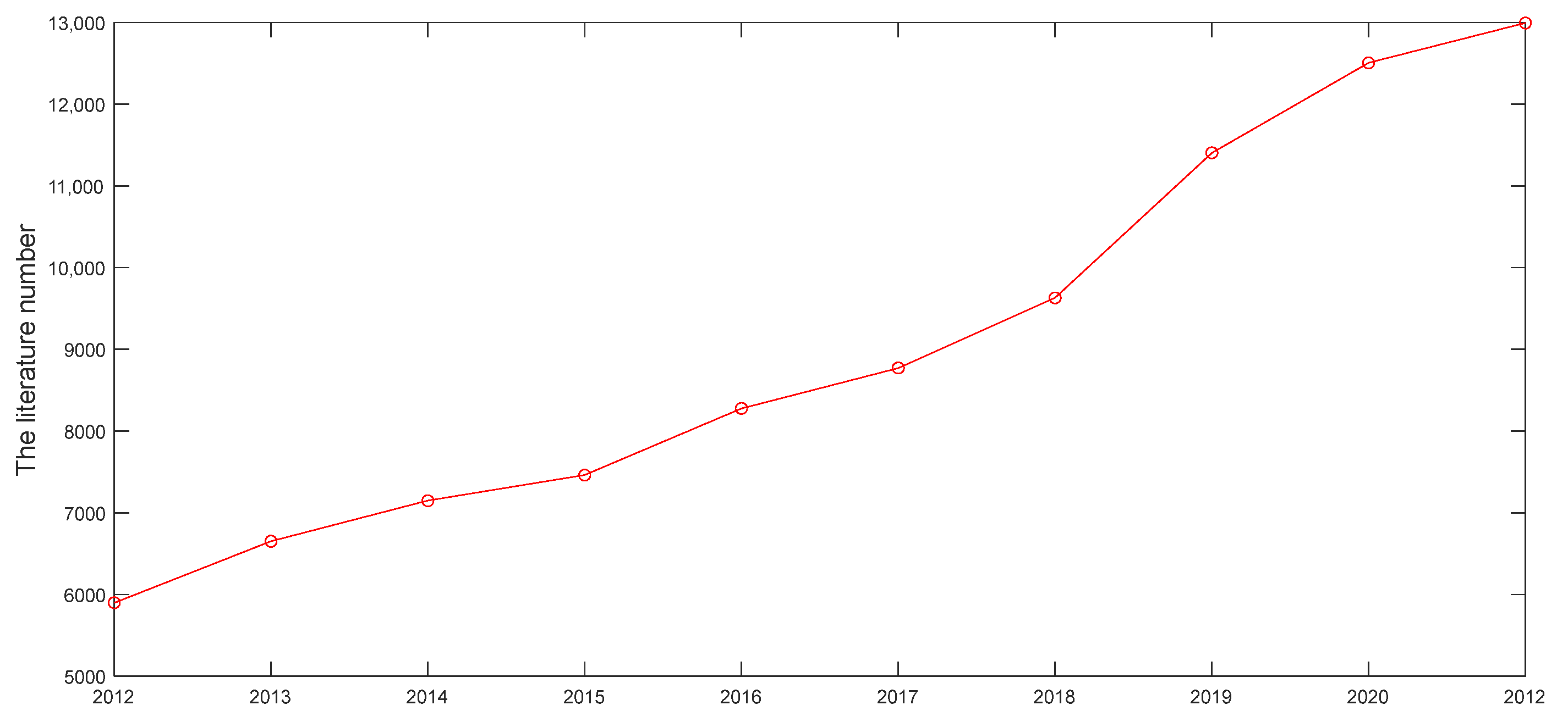
As the cornerstone of economic development and industrial progress, energy plays a significant role. Due to environmental pollution [1,2], instability of clean energy, and other reasons, energy prediction has become a very important research content, including energy consumption [3] and energy production [4]. According to data released by the National Energy Bureau, China’s energy consumption and production have been on the rise in recent years. However, energy consumption tends to be greater than energy production, and China needs to rely on energy imports to maintain the balance between the two. However, not all energy has the characteristic of inexhaustible; all countries in the world advocate sustainable development strategy. In this context, energy prediction must be made. Energy forecasting is the advance planning of the future energy market, an important means to maintain the balance between supply and demand in the market, reduce the waste of resources, and provide technical support for the implementation of sustainable development strategy. However, influenced by many uncertain factors, monthly and quarterly energy time series often show more data characteristics, such as seasonality and nonlinearity. Thus, compared with annual series forecast, monthly and quarterly series forecasting can provide more detailed suggestions for relevant planning. In addition, taking Web of Science as an example, we set the theme as “energy prediction” to search the literature in the last 10 years. As can be observed in Figure 1, the number of articles on energy forecasting is increasing every year, and most of the growth trends are in an upward state. Therefore, energy prediction has been a hot issue, and its research is of great significance. At present, there are three main methods for energy prediction, which are statistical models, machine learning models, and grey prediction models.

1.1. Energy Forecasting Model

The ARIMA model and SARIMA model, as classical models in statistical econometric models, are common methods for energy forecasting. Wang et al. established the ARIMA model for short-term prediction analysis of coal price and proved the utility of the model [5]. In view of the long memory of coal consumption, Liu et al. proposed the application of a fractional difference ARIMA model to make the predicted value closer to the actual value [6]. The SARIMA model is commonly used for energy data with seasonal fluctuation. Dabral et al. used SARIMA to predict month, week and day sequences, and obtained good results [7]. Based on the SARIMA model, Sigauke et al. proposed the Reg-SARIMA-GARCH model, which was successfully applied to peak demand of daily electricity in South Africa [8]. The research on the ARIMA model and SARIMA model is more than that. Better prediction results can be obtained by improving the existing model, including wavelet transform [9], RTS smoothing algorithm [10], genetic algorithm [11], etc. Additionally, the prediction effect of some combination methods is also better than that of a single statistical econometric model [12,13]. The statistical econometric models can predict well in many cases, but they are mostly used to describe linear structure sequences. In addition, such models require a large number of sample data to get high-precision results, and the data are required to meet certain distribution rules. Not all of these requirements can be satisfied in energy forecasting.

Machine learning models are used extensively since they can deal with the complexity and nonlinearity of energy systems. The BP neural network model, an important model in machine learning model, originates from imitating the function of the human brain. Wang et al. found the most suitable neural network by comparing network structures and cross-validation, and used it to predict solar irradiance [14]. Further, Wen et al. made a double improvement on the particle swarm optimization algorithm to propose DPSO-BP model. The results show that the prediction effect of the new model is better than that of the single BP neural network model [15]. However, the BP neural network model relies too much on the input data of the model and is easy to fall into local optimization, while the SVR model can solve this problem better. Ning et al. proposed the ε-SVR prediction model based on rolling time window, which improved the accuracy of coal price prediction model [16]. With the deepening of research, many research results show that the combination of SVR model and intelligent algorithm can effectively improve the model accuracy, including particle swarm optimization algorithm [17], genetic algorithm [18], Grey–Wolf optimizer [19], chaotic artificial bee colony algorithm [20], whale optimization algorithm [21], etc., further expanding the application scope of SVR model. As a derivative of the SVM model, the LSSVR model has the same utility as SVR model. Wei et al. used the optimized GA-LSSVM model to gain high-precision power load prediction results [22]. Besides the above models, ANN is also a common machine learning model. Khwaja et al. applied the ANN model to monthly power load prediction in order to reduce the prediction error [23]. Machine learning models effectively capture the nonlinear characteristics of the data, but they also need a large number of sample data to run. In addition, the relevant control parameters of the model need to be set before using, which adds complexity.

Limited by the requirements of data volume and data distribution, the use of grey system models for prediction is excellent. They have low data requirements and can be widely used in prediction of different types of data. Before the prediction, the grey operator is used to deal with the system, which is the basis of the grey prediction model. As a classical operator in grey prediction theory, the grey one-order accumulation generation operator created by Deng Julong can smooth original data and find internal laws of data more effectively [24]. In recent years, in order to improve the prediction accuracy, the research on grey operator has gradually increased. Based on the principle of “new information priority”, Wu et al. established fractional accumulation operators to solve the contradiction between the low-impact solution of new data and the principle of “new information priority” [25]. On this basis, fractional accumulation operators have been implemented in many models, such as ${\mathrm{GM}}^{\frac{p}{q}}\left(1,1\right)$ [26], ${\mathrm{GM}}^{\frac{p}{q}}\left(2,1\right)$ [27], and ${\mathrm{NDGM}}^{\frac{p}{q}}\left(1,1\right)$ [28], etc. Consequently, fractional accumulation operators have attracted wide attention. Zeng et al. introduced fractional accumulation operators into the GM(2,1) model and got effective prediction results in numerical simulation experiments and application examples [29]. For the purpose of realizing the maximum data mining in a small amount of information, Jiang et al. built a fractional reverse accumulation nonlinear grey Bernoulli model so that the accuracy of the model improved [30]. In addition to single-variable models, fractional accumulation operators can also produce good performance in multivariable models. After comprehensively considering various factors affecting the system, Zhang et al. proposed a multivariable fractional grey model to get more accurate prediction results [31]. The existing fractional accumulation operator directly accumulates data but it may not reflect the hidden periodic volatility of the sequence. Based on this, a new fractional periodic accumulation operator is proposed to improve it. This operator accumulates within each cycle, not the overall accumulation. It not only fully excavates the data law, but also retains the periodic fluctuation of the accumulated data.

The grey operator can deeply dig into data rules and improve the prediction effect, but the choice of model also plays a key role in improving the prediction effect. Considering the scarcity, complexity, and nonlinearity of the energy sequence, Wang et al. [32] proposed a new fractional time-delayed grey Bernoulli model and verified the validity of the new model in three energy-related cases. Liu et al. [33] constructed an optimized grey system model with weighted fractional accumulation generation operation, and proved the validity of the proposed model by using the natural gas production of Germany, Italy, and Canada. Finally, the new model was used to predict natural gas production in China. Liu et al. proposed an FPGM(1,1,t^a) model based on the combination of time power term and fractional accumulation operator to predict electricity consumption in India and China [34]. The use of electric vehicles represents an effective method to alleviate energy shortage and environmental problems. Ding et al. proposed a new self-adaptive optimized grey model which plays an effective role in the annual series prediction of electric vehicles [35]. Most of the annual energy time series are in a single development trend, which cannot fully show the data law. However, monthly and quarterly energy time series show seasonal and nonlinear characteristics. In order to further analyze the laws of energy data in further detail, many studies have been conducted on these two characteristics in order to provide more refined management of energy planning. Seasonality is mainly dealt with through specific methods, including the following six common methods: seasonal factor [36], dynamic seasonal adjustment factor [37], dummy variable [38], data grouping method [39], CTAGO [40], and cycle accumulation operation [41]. It turns out that using these methods can effectively eliminate the seasonality of a sequence by adding additional parameters or steps. Subsequently, Wu et al. combined the fractional accumulation operator with the Holt–Winters model, and the grey Holt–Winters model constructed could describe the seasonality of the sequence without any processing. The case analysis shows that this model has superior performance [42]. The grey Holt–Winters model focuses on describing the seasonal characteristics of the sequence, but does not highlight the nonlinear characteristics of the sequence. In view of nonlinear characteristics, Zheng et al. introduced an unbiased NGBM model based on the NGBM model to predict China’s hydropower consumption [43]. Ding et al. introduced grey power indexes into the model structure to construct a new discrete grey power model and obtained effective results in the empirical analysis [44]. Qian et al. proposed a new structure self-adaptive discrete grey prediction model, which effectively described the nonlinear and linear characteristics of the sequence [45]. Considering the nonlinear problem of nuclear energy consumption, Ding et al. applied a novel structure-adaptive grey model to predict the nuclear energy consumption cases in China and the United States and verified the effectiveness of the new model [46]. In order to better predict the sequence of nuclear energy consumption, Ding et al. re-developed an optimized structure-adaptive grey model. The results showed that the new model had better prediction results [47]. Zhou et al. constructed an SNGBM(1,1) model based on Bernoulli equation with nonlinear structure, which can successfully consider nonlinear and seasonal characteristics in the sequence [48]. Further, Zhou et al. combined dummy variables, the framework of LSSVR model and grey accumulation operator to propose GSLSSVR model and successfully applied it to practical cases [49]. These grey models can obtain satisfactory results in prediction and have different processing methods for seasonal and nonlinear characteristics of the sequence. However, there may be deficiencies in the processing process, which mainly have two aspects. On the one hand, seasonal and nonlinear characteristics of monthly and quarterly energy time series appear simultaneously. Addressing the two features separately may produce certain errors. On the other hand, the two features are processed simultaneously, but related feature parameters are added to the model structure. The calculation is added in the later model solving process, which may cause some errors.

1.2. The Motivation of This Work

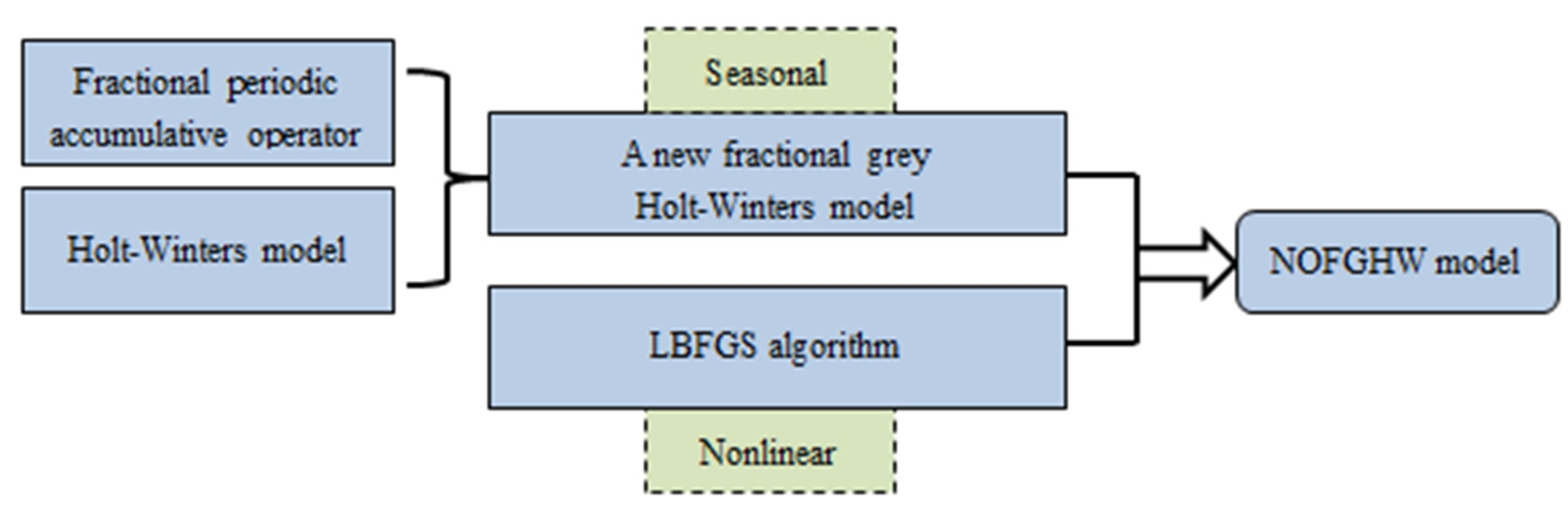
Considering the integrity of monthly and quarterly energy time series, this paper proposes a new fractional grey Holt–Winters model, namely the NOFGHW model, to further explore the internal laws of energy data. In the new model, a new fractional periodic accumulation operator is proposed based on the existing fractional accumulation operator. Originally, this operator not only embodies the principle of “new information priority”, but also preserves the periodic fluctuation of data. Then, the new operator is combined with the Holt–Winters model. The Holt–Winters model can identify seasonality in a sequence. Finally, parameters in the Holt–Winters model and the new operator are optimized by LBFGS algorithm in a quasi-Newton method. The largest advantage of this algorithm is that it can deal with nonlinear problems. Figure 2 shows the combination of the new model. The new model can deal with the seasonal and nonlinear problems in the sequence at the same time without adding additional parameters related to the sequence characteristics. In order to verify the effectiveness of the new model, this paper applies the new model to monthly crude oil production and quarterly industrial electricity consumption, respectively. The main innovations of this paper are as follows:

(1) Based on the existing fractional accumulation operators, a new fractional periodic accumulation operator is proposed in this paper, which has the principle of “new information priority”. This operator fully retains the periodic fluctuation of the accumulated data and can effectively mine the characteristics of monthly and quarterly energy data.

(2) A new optimization method (LBFGS algorithm) is used to find parameters in the model. This algorithm is a common method to solve nonlinear problems. It is widely used due to its fast convergence speed and small memory occupation.

(3) Starting from the Holt–Winters model, which can recognize the seasonal characteristics of sequences, this paper combines it with the new fractional periodic accumulation operator, and uses the LBFGS algorithm to optimize parameters. In the calculation process, only the parameters contained in the Holt–Winters model and the order of fractional periodic accumulation operator need to be calculated to describe the seasonal and nonlinear characteristics of monthly and quarterly energy data at the same time. As a result, the feature parameters previously added for processing sequence features are reduced, and the calculation for describing sequence features is reduced. The new model constructed in this paper provides a simpler method for the prediction of energy time series. The new model constructed in this paper provides a more convenient method for predicting energy time series.

(4) In the validation stage of the new model, this paper selects two energy cases, namely monthly crude oil output and quarterly industrial electricity consumption. These two cases have the following three characteristics, respectively, including different seasonal (different degrees), different cycles (monthly and quarterly), and different energy types (energy production and energy consumption). By analyzing the two cases one by one, it can be found that the overall effect of the new model is better than that of the comparison model, which indicates that the model can be widely used in different cases of energy prediction. Hence, the adaptability of the new model is verified.

The rest of this paper is shown below. In Section 2, the new model NOFGHW, LBFGS algorithm and corresponding evaluation criteria are introduced in detail. In Section 3, two empirical cases and solving methods of six model parameters are introduced. Then, the model results are analyzed to prove the superiority of the new model. Section 4 presents a summary of the whole paper and future work.

2. Methods

This section discusses the construction process of the new optimized fractional grey Holt–Winters model (NOFGHW). The new model is composed of the new fractional periodic accumulation operator, the Holt–Winters model, and the LBFGS algorithm, which fully demonstrates the advantages of each part. In addition, this section also introduces the procedure of using LBFGS algorithm and the corresponding model evaluation criteria. The meanings of symbols, constraints, and variables that appear in this section are tabulated in the Appendix A.

2.1. A New Optimized Fractional Grey Holt-Winters Model (NOFGHW)

Step 1. Suppose that $X^{\left(0\right)}=\left(x^{\left(0\right)}\left(1\right),x^{\left(0\right)}\left(2\right),x^{\left(0\right)}\left(3\right),\dots ,x^{\left(0\right)}\left(n\right)\right)$ is a nonnegative primitive sequence with seasonality and nonlinearity, and the period is $L\left(L=4 or L=12\right)$. Then, the r-order accumulation sequence can be obtained by fractional periodic accumulation operator, which is recorded as $X^{\left(r\right)}=\left(x^{\left(r\right)}\left(1\right),x^{\left(r\right)}\left(2\right),\dots ,x^{\left(r\right)}\left(n\right)\right)$. The fractional periodic accumulation operator is expressed as:

$$x^{\left(r\right)}\left(k\right)={\displaystyle \sum _{i=\left(\lceil k/L\rceil -1\right)L+1}^k\frac{\Gamma \left(r+k-i\right)}{\Gamma \left(k-i+1\right)\Gamma \left(r\right)}{x}^{\left(0\right)}\left(i\right),k=1,2,3,\dots ,n}$$

(1)

where $\lceil k/L\rceil$ represents an integer not less than $k/L$ and $r$ represents fractional order.

The corresponding reduction formula can be expressed as:

$$x^{\left(0\right)}\left(k\right)=\{\begin{array}{ll}{\left(x^{\left(r\right)}\right)}^{\left(-r\right)}\left(k\right)={\displaystyle \sum _{i=0}^{\left(k\mathrm{mod}L\right)-1}{\left(-1\right)}^i\frac{\Gamma \left(r+1\right)}{\Gamma \left(i+1\right)\Gamma \left(r-i+1\right)}{x}^{\left(r\right)}\left(k-i\right)}& k\mathrm{mod}L\ne 0,1\\ {\left(x^{\left(r\right)}\right)}^{\left(-r\right)}\left(k\right)={\displaystyle \sum _{i=0}^{\left(k\mathrm{mod}L\right)+3}{\left(-1\right)}^i\frac{\Gamma \left(r+1\right)}{\Gamma \left(i+1\right)\Gamma \left(r-i+1\right)}{x}^{\left(r\right)}\left(k-i\right)}& k\mathrm{mod}L=0\\ x^{\left(r\right)}\left(k\right)& k\mathrm{mod}L=1\end{array},$$

(2)

Step 2. Establish NOFGHW model.

$$\begin{array}{ll}{S}_k=\alpha \frac{x^{\left(r\right)}\left(k\right)}{C_{k-L}}+\left(1-\alpha \right)\left(S_{k-1}+b_{k-1}\right),0<\alpha <1& \\ b_k=\beta \left(S_k-S_{k-1}\right)+\left(1-\beta \right)b_{k-1},0<\beta <1,& k=L+1,L+2,\dots ,n\\ C_k=\gamma \frac{x^{\left(r\right)}\left(k\right)}{S_k}+\left(1-\gamma \right)C_{k-L},0<\gamma <1& \end{array}$$

(3)

The initial value of the model is

$$\begin{array}{l}{S}_L=x^{\left(r\right)}\left(L\right);\\ C_i=\frac{x^{\left(r\right)}\left(i\right)}{\frac{{\displaystyle \sum _{j=1}^L{x}^{\left(r\right)}\left(j\right)}}{L}},i=1,2,3,\dots ,L;\\ b_L=\frac{1}{L}\left(\frac{x^{\left(r\right)}\left(L+1\right)-x^{\left(r\right)}\left(1\right)+x^{\left(r\right)}\left(L+2\right)-x^{\left(r\right)}\left(2\right)+\cdots +x^{\left(r\right)}\left(L+L\right)-x^{\left(r\right)}\left(L\right)}{L}\right).\end{array}$$

(4)

where $\alpha$ is data smoothing factor, $\beta$ is trend smoothing factor, $\gamma$ is the seasonal change smoothing factor, $S$ denotes level, $b$ denotes trend, and $C$ denotes seasonal.

Step 3. The new model has four parameters, namely, fractional order $r$, data smoothing factor $\alpha$, trend smoothing factor $\beta$ and seasonal change smoothing factor $\gamma$. We use the LBFGS algorithm in the quasi-Newton method to optimize them, which is described in detail in the section of parameter optimization of NOFGHW model. Then, we can get the parameters $D=\left[\widehat{\alpha },\widehat{\beta },\widehat{\gamma },\widehat{r}\right]$. Based on this, the prediction formula of the new model can be deduced as:

$${\widehat{F}}^{\left(r\right)}\left(k+m\right)=\left(S_k+m{b}_k\right)C_{k-L+1+\left(m-1\right)\mathrm{mod}L}$$

(5)

where m is the number of recursions.

Step 4. The simulation and prediction results obtained in Step 3 are reduced by Formula (2).

$${\widehat{F}}^{\left(0\right)}\left(k+m\right)=\{\begin{array}{ll}{\left({\widehat{F}}^{\left(r\right)}\right)}^{\left(-r\right)}\left(k+m\right)={\displaystyle \sum _{i=0}^{\left(\left(k+m\right)\mathrm{mod}L\right)-1}{\left(-1\right)}^i\frac{\Gamma \left(r+1\right)}{\Gamma \left(i+1\right)\Gamma \left(r-i+1\right)}{\widehat{F}}^{\left(r\right)}\left(k+m-i\right)\left(k+m\right)}& \mathrm{mod}L\ne 0,1\\ {\left({\widehat{F}}^{\left(r\right)}\right)}^{\left(-r\right)}\left(k+m\right)={\displaystyle \sum _{i=0}^{\left(\left(k+m\right)\mathrm{mod}L\right)+3}{\left(-1\right)}^i\frac{\Gamma \left(r+1\right)}{\Gamma \left(i+1\right)\Gamma \left(r-i+1\right)}{\widehat{F}}^{\left(r\right)}\left(k+m-i\right)\left(k+m\right)}& \mathrm{mod}L=0,\\ {\widehat{F}}^{\left(r\right)}\left(k+m\right)\left(k+m\right)& \mathrm{mod}L=1\end{array}$$

(6)

2.2. Parameter Optimization of NOFGHW Model

2.2.1. Parameter Optimization Calculation Process

In this paper, the data of in-sample simulation stage are used to optimize the parameters, and then the obtained parameters are used to predict the new model. In order to get the most suitable parameters, we use the following calculation process in the optimization. According to the calculation process in Section 2.1, the first L data are not simulated, and the simulation stage starts from $L+1$.

The first is the simulated values from $L+1$ to $L+L$:

$$\begin{array}{ll}{\widehat{F}}^{\left(r\right)}\left(L+1\right)=\left(S_L+b_L\right)C_1;& \\ {\widehat{F}}^{\left(r\right)}\left(L+2\right)=\left(S_{L+1}+b_{L+1}\right)C_2& =[\left(1+\beta \right)\alpha \frac{x^{\left(r\right)}\left(L+1\right)}{C_1}\\ & +\left(1-\alpha -\alpha \beta \right)S_L+\left(2-\alpha -\alpha \beta \right)b_L]C_2;\\ {\widehat{F}}^{\left(r\right)}\left(L+3\right)=\left(S_{L+2}+b_{L+2}\right)C_3& =[\left(1+\beta \right)\alpha \frac{x^{\left(r\right)}\left(L+2\right)}{C_2}\\ & +\left(1-\alpha -\alpha \beta \right)S_{L+1}+\left(2-\alpha -\alpha \beta \right)b_{L+1}]C_3;\\ & ⋮\\ {\widehat{F}}^{\left(r\right)}\left(L+L\right)=\left(S_{L+L-1}+b_{L+L-1}\right)C_L& =[\left(1+\beta \right)\alpha \frac{x^{\left(r\right)}\left(L+L-1\right)}{C_{L-1}}\\ & +\left(1-\alpha -\alpha \beta \right)S_{L+L-2}+\left(2-\alpha -\alpha \beta \right)b_{L+L-2}]C_L;\end{array}$$

Then from $2L+1$ to $\left(i+1\right)L+t$:

$$\begin{array}{lll}{\widehat{F}}^{\left(r\right)}\left(L+L+1\right)& =& [\left(1+\beta \right)\alpha \frac{x^{\left(r\right)}\left(L+L\right)}{C_L}+\left(1-\alpha -\alpha \beta \right)S_{L+L-1}\\ & & +\left(2-\alpha -\alpha \beta \right)b_{L+L-1}]C_{L+1}\\ & =& \left(1+\beta \right)\alpha x^{\left(r\right)}\left(L+L\right)\frac{\gamma x^{\left(r\right)}\left(L+1\right)+\left(1-\gamma \right)C_1{S}_{L+1}}{C_1{S}_{L+1}}\\ & & +\left(1-\alpha -\alpha \beta \right)[\gamma \frac{S_{L+L-1}{x}^{\left(r\right)}\left(L+1\right)}{S_{L+1}}+\left(1-\gamma \right)C_1{S}_{L+L-1}]\\ & & +\left(2-\alpha -\alpha \beta \right)[\gamma \frac{x^{\left(r\right)}\left(L+1\right)b_{L+L-1}}{S_{L+1}}+\left(1-\gamma \right)C_1{b}_{L+L-1}];\\ {\widehat{F}}^{\left(r\right)}\left(L+L+2\right)& =& [\left(1+\beta \right)\alpha \frac{x^{\left(r\right)}\left(L+L+1\right)}{C_{L+1}}+\left(1-\alpha -\alpha \beta \right)S_{L+L}\\ & & +\left(2-\alpha -\alpha \beta \right)b_{L+L}]C_{L+2}\\ & =& \left(1+\beta \right)\alpha x^{\left(r\right)}\left(L+L+1\right)\frac{S_{L+1}[\gamma x^{\left(r\right)}\left(L+2\right)+\left(1-\gamma \right)C_2{S}_{L+2}]}{S_{L+2}[\gamma x^{\left(r\right)}\left(L+1\right)+\left(1-\gamma \right)C_1{S}_{L+1}]}\\ & & +\left(1-\alpha -\alpha \beta \right)[\gamma \frac{S_{L+L}{x}^{\left(r\right)}\left(L+2\right)}{S_{L+2}}+\left(1-\gamma \right)S_{L+L}{C}_2]\\ & & +\left(2-\alpha -\alpha \beta \right)[\gamma \frac{x^{\left(r\right)}\left(L+2\right)b_{L+L}}{S_{L+2}}+\left(1-\gamma \right)b_{L+L}{C}_2];\\ & & ⋮\\ {\widehat{F}}^{\left(r\right)}\left(L+iL+t\right)& =& [\left(1+\beta \right)\alpha \frac{x^{\left(r\right)}\left(L+iL+t-1\right)}{C_{iL+t-1}}+\left(1-\alpha -\alpha \beta \right)S_{L+iL+t-2}\\ & & +\left(2-\alpha -\alpha \beta \right)b_{L+iL+t-2}]C_{iL+t}\\ & =& \left(1+\beta \right)\alpha x^{\left(r\right)}\left(L+iL+t-1\right)\frac{S_{iL+t-1}[\gamma x^{\left(r\right)}\left(iL+t\right)+\left(1-\gamma \right)C_t{S}_{iL+t}]}{S_{iL+t}[\gamma x^{\left(r\right)}\left(iL+t-1\right)+\left(1-\gamma \right)C_{t-1}{S}_{iL+t-1}]}\\ & & +\left(1-\alpha -\alpha \beta \right)[\gamma \frac{S_{L+iL+t-2}{x}^{\left(r\right)}\left(iL+t\right)}{S_{iL+t}}+\left(1-\gamma \right)S_{L+iL+t-2}{C}_t]\\ & & +\left(2-\alpha -\alpha \beta \right)[\gamma \frac{x^{\left(r\right)}\left(iL+t\right)b_{L+iL+t-2}}{S_{iL+t}}+\left(1-\gamma \right)b_{L+iL+t-2}{C}_t];\end{array}$$

where $i\in \left[1,\frac{number of data in the simulation phase}{L}-2\right]$, $t\in \left[1,L\right]$.

From the above derivation process, it can be found that the derivation formula of $L+1$ to $L+L$ stage is different from that of the subsequent stage, which needs to be listed separately. This is due to the fact that according to Formulas (3) and (4) in Section 2.2, it can be found that $C_1$ to $C_L$ are known and there is no need for iterative calculation. In the latter stage, $C$ is unknown and needs to be generated by formula iteration for calculation.

2.2.2. Parameter Optimization Process

The LBFGS algorithm can deal with unconstrained nonlinear problems. In the process of calculation, it will delete the content stored in the previous stage and replace it with the updated content as required. Therefore, LBFGS algorithm does not occupy a large amount of memory. The detailed steps of optimization parameters of the algorithm are as follows:

Step 1: Setting the initial vector $x0$, memory size $w$ and the number of iterations $l=0$;

Step 2: Calculating the first step degree $g$ and search direction $d$ of the function;

Step 3: The step size ${\alpha }_s$ is obtained according to the strong wolfe criterion;

Step 4: In terms of the above results, the inverse $Hg$ of Hessian matrix is calculated;

Step 5: Carrying out the next iteration and judging whether the stop conditions are met. Otherwise, return to step 2.

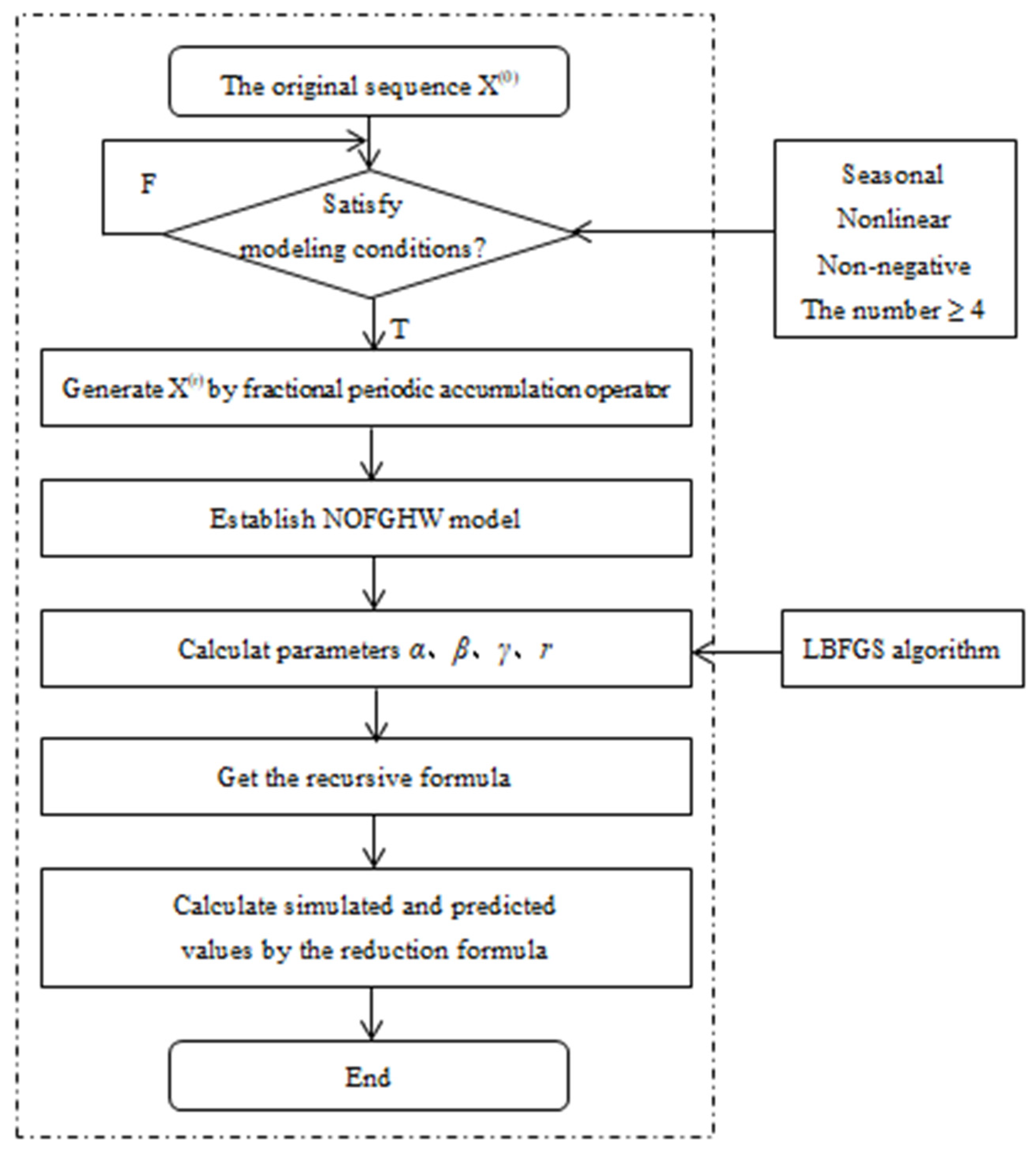
To further intuitively understand the prediction process of NOFGHW model under LBFGS optimization, we made a flow chart (as shown in Figure 3).

2.3. Evaluation Criteria

In order to compare the performance of the model more clearly, this paper adopts the following five methods to evaluate the effect of the model, which are average percentage error (APE), average absolute percentage error (MAPES, MAPSP), root mean square error (RMSES, RMSEP). The formula is as follows:

$$\mathrm{APE}\left(k\right)=\left|\frac{{\widehat{F}}^{\left(0\right)}\left(k\right)-x^{\left(0\right)}\left(k\right)}{x^{\left(0\right)}\left(k\right)}\right|\ast 100\%,k=1,2,3,\dots ,n+p$$

$$\mathrm{MAPES}=\frac{1}{n}{\displaystyle \sum _{k=1}^n\mathrm{APE}\left(k\right),\mathrm{MAPES}=\frac{1}{p}{\displaystyle \sum _{k=n+1}^{n+p}\mathrm{APE}\left(k\right)}}$$

$$\mathrm{RMSES}=\sqrt{\frac{1}{n}{\displaystyle \sum _{k=1}^n{\left({\widehat{F}}^{\left(0\right)}\left(k\right)-x^{\left(0\right)}\left(k\right)\right)}^2}},\mathrm{RMSEP}=\sqrt{\frac{1}{p}{\displaystyle \sum _{k=n+1}^{n+p}{\left({\widehat{F}}^{\left(0\right)}\left(k\right)-x^{\left(0\right)}\left(k\right)\right)}^2}}$$

where n is sample size and p is the forecasted horizon.

3. Application

To further demonstrate the performance of the new model when predicting a series with seasonal and nonlinear characteristics, this section uses two cases of monthly crude oil production and quarterly industrial electricity consumption to evaluate the performance of the new model. As an energy in energy production, crude oil production has obvious seasonality and nonlinearity, which can effectively verify the effect of the new model. Although industrial electricity consumption is not as seasonal as crude oil production, this case further proves the flexibility of the new model in dealing with different degrees of seasonality. Furthermore, crude oil production is a monthly case and industrial electricity consumption is a quarterly case, which can verify the effectiveness of the new model in sample data of different periods. In addition, these two cases have clearly opposite characteristics, one representing energy production and the other representing energy consumption. By studying these two cases, one positive and one negative, the effectiveness of the new model in energy applications can be fully verified.

3.1. The Experiment Design

In the above analysis, the data of the two cases we use are from Statistics database of China Economic Network Statistics database (https://db.cei.cn/ (accessed on 4 February 2022)). In the case of monthly crude oil, the cycle is set to eleven, since many domestic data aggregate the data from January to February during the Spring Festival into an accumulated value. We use 2000–2018 as the in-sample simulation phase and 2019–2020 as the out-of-sample prediction phase. In the case of quarterly industrial power consumption, the period is set to four. We use 2011–2018 as the in-sample simulation phase and 2019–2020 as the out-of-sample prediction phase. These collected data play a supporting role in case studies. In addition, in order to clearly show the effect of the new model, we selected OGHW, SNGBM, SARIAM, LSSVR, and BPNN as comparison models. Among them, the OGHW is a model formed by combining grey one-order accumulation operator with the Holt–Winters model and optimizing parameters with the LBFGS algorithm. The SNGBM model is a grey forecasting model with better effect in seasonal and nonlinear forecasting, while the SARIMA model is a common model in statistical econometric models. The LSSVR model is better at dealing with the nonlinearity of sequence. Both the LSSVR model and BPNN model are machine learning models.

3.2. Parameter Solution

In this section, we make simulations and predictions based on the data collected in Section 3.1. At the same time, we obtain some parameters for the six models in Section 3.1. The parameters in the model are explained through the crude oil production case, while the parameters of the industrial electricity consumption case are shown in the Appendix.

Table 1. Detailed parameters of all models of crude oil production cases.

Models	Parameters
NOFGHW	$\widehat{\alpha }$= 7263, $\widehat{\beta }$= 0.0070, $\widehat{\gamma }$= 0.6832, $\widehat{r}$= 0.1679.
OGHW	$\widehat{\alpha }$= 0.5881, $\widehat{\beta }$= 0.0000, $\widehat{\gamma }$= 0.6189.
SNGBM	fs(1) = 1.7815, fs(2) = 0.9333, fs(3) = 0.9015, fs(4) = 0.9333, fs(5) = 0.9179, fs(6) = 0.9262, fs(7) = 0.9307, fs(8) = 0.9023, fs(9) = 0.9332, fs(10) = 0.9081, fs(11) = 0.9319, A = [0.0015, 262.5373], r = 0.1707.
SARIMA	SARIMA(1,0,10)(0,1,0)11, AR(1) = −0.2940 ***, MA(10) = −0.1331 *, AIC = -4.9214, Log L = 487.7607.
LSSVR	Embedding dimensions = 11, time lag = 1, linear kernel, γ∈[0.0826, 270,104.1352], the optimalγ= 12.2672, α1= −0.1075, α2= 0.0948, …, α196= 1.0788, b = −4.8779.
BPNN	Optimal embedding dimensions = 11, optimal time lag = 1, number of neurons = 20, learning rate = 0.01, iterative number = 1000, error goal = 0.05.

Note: (*), (**) and (***) represent the significance levels of the coefficients of 10%, 5% and 1% respectively.

shows the detailed parameters of all models in the crude oil case. Among them, the NOFGHM model and the OGHW model (The OGHW is a model formed by combining grey one-order accumulation operator with the Holt–Winters model and optimizing parameters with LBFGS algorithm.) are optimized by the LBFGS algorithm introduced in Section 2.2 to obtain model parameters $\alpha ,\beta ,\gamma$. The seasonal fluctuation index $f_s$ in the SNGBM model was calculated by the average method, and the parameter A was obtained by the least square method. The index $r$ in SNGBM is optimized by cultural algorithm. The SARIAM model is implemented in EVIEWS software. Both the LSSVR model and the BPNN model are in the form of multi-dimensional input and single-dimensional output. Therefore, we need to transform the input single-dimensional sequence into multi-dimensional data through phase space transformation. In addition, the embedding dimension and delay time used in the conversion need to be selected and set.

3.3. Result Analysis

3.3.1. Monthly Crude Oil Production

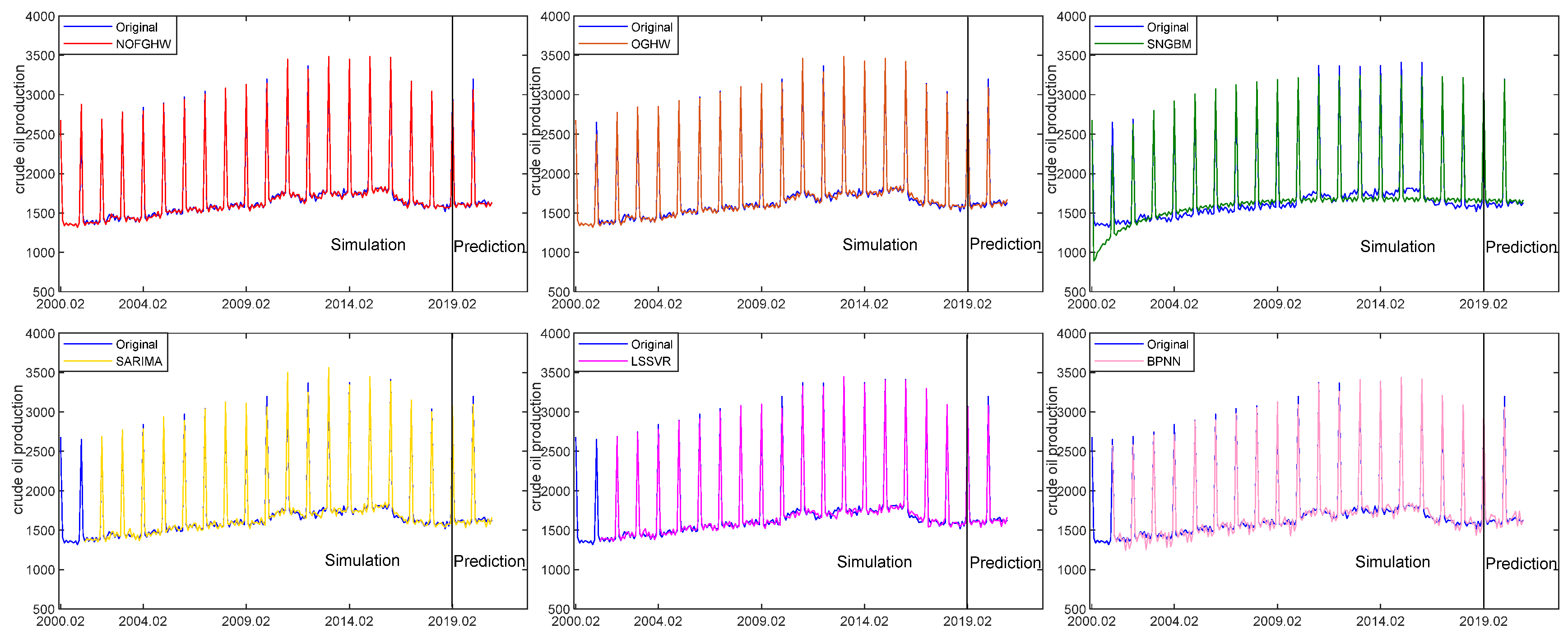
Crude oil is an important energy source, and its product plays an important role in industry, agriculture, and other fields (such as fuel for transportation, chemical raw materials, etc.). Additionally, oil demand fell during the severe phase of the COVID-19 pandemic, but as governments around the world control this pandemic, oil consumption is gradually returning to the a prosperous stage. In China, domestic crude oil production cannot meet specified requirements, so there is a need to import a lot of crude oil from abroad. Based on this, we must pay attention to the production of crude oil to avoid the imbalance between supply and demand. In this paper, NOFGHW model and the five comparison models mentioned in Section 3.1 are used for prediction, and the evaluation criteria in Section 2.3 are used to test the effect of the model (as shown in Figure 4 and Figure 5,

Table 2. Forecast value of crude oil production (Unit: 10,000 tons), APE(%), MAPE(%), RMSE(%).

Month	Actual	NOFGHW	APE	OGHW	APE	SNGBM	APE	SARIMA	APE	LSSVR	APE	BPNN	APE
2019-M2	3069.20	3051.23	0.59	3051.15	0.59	3207.97	4.52	3073.44	0.14	3061.05	0.27	3099.15	0.98
2019-M3	1654.20	1615.10	2.36	1597.72	3.41	1679.97	1.56	1617.73	2.20	1613.78	2.44	1655.62	0.09
2019-M4	1571.10	1570.24	0.05	1549.32	1.39	1622.14	3.25	1568.09	0.19	1569.97	0.07	1597.37	1.67
2019-M5	1623.00	1623.01	0.00	1601.67	1.31	1678.74	3.43	1616.62	0.39	1617.55	0.34	1635.72	0.78
2019-M6	1610.00	1608.55	0.09	1595.52	0.90	1650.31	2.50	1604.09	0.37	1605.23	0.30	1697.48	5.43
2019-M7	1628.70	1611.09	1.08	1604.94	1.46	1664.70	2.21	1599.27	1.81	1605.11	1.45	1674.46	2.81
2019-M8	1618.20	1613.10	0.32	1610.41	0.48	1672.11	3.33	1618.24	0.00	1619.85	0.10	1678.36	3.72
2019-M9	1564.30	1567.22	0.19	1566.26	0.13	1620.39	3.59	1529.98	2.19	1533.93	1.94	1523.43	2.61
2019-M10	1611.30	1626.84	0.96	1634.94	1.47	1675.22	3.97	1626.14	0.92	1627.51	1.01	1643.76	2.01
2019-M11	1570.40	1583.07	0.81	1597.31	1.71	1629.55	3.77	1562.84	0.48	1569.76	0.04	1533.80	2.33
2019-M12	1606.50	1625.73	1.20	1649.56	2.68	1671.63	4.05	1645.45	2.42	1649.85	2.70	1550.02	3.52
2020-M2	3200.20	3065.48	4.21	3091.70	3.39	3194.25	0.19	3095.06	3.29	3080.38	3.74	3058.90	4.42
2020-M3	1656.30	1622.20	2.06	1618.92	2.26	1672.71	0.99	1629.31	1.63	1624.52	1.92	1611.62	2.70
2020-M4	1587.47	1577.21	0.65	1569.86	1.11	1615.05	1.74	1579.26	0.52	1582.85	0.29	1574.74	0.80
2020-M5	1645.60	1630.30	0.93	1622.88	1.38	1671.32	1.56	1628.15	1.06	1631.81	0.84	1633.20	0.75
2020-M6	1624.20	1615.80	0.52	1616.63	0.47	1642.94	1.15	1615.52	0.53	1620.25	0.24	1650.67	1.63
2020-M7	1646.30	1618.39	1.70	1626.14	1.22	1657.19	0.66	1610.67	2.16	1619.36	1.64	1689.07	2.60
2020-M8	1665.10	1620.44	2.68	1631.65	2.01	1664.49	0.04	1629.78	2.12	1634.90	1.81	1738.22	4.39
2020-M9	1609.60	1574.34	2.19	1586.90	1.41	1612.93	0.21	1540.89	4.27	1545.37	3.99	1553.22	3.50
2020-M10	1641.20	1634.29	0.42	1656.46	0.93	1667.44	1.60	1637.73	0.21	1641.49	0.02	1742.17	6.15
2020-M11	1596.50	1590.32	0.39	1618.31	1.37	1621.90	1.59	1573.98	1.41	1581.67	0.93	1566.23	1.90
2020-M12	1626.80	1633.20	0.39	1671.22	2.73	1663.71	2.27	1657.17	1.87	1662.15	2.17	1620.91	0.36
MAPES			1.2490		1.3831		4.8086		1.5667		1.5794		2.4277
RMSES			33.6778		34.3136		103.3027		38.6412		37.4124		51.8965
MAPEP			1.0808		1.5364		2.1898		1.3725		1.2839		2.5069
RMSEP			34.9260		35.1592		48.3058		34.4965		35.8055		55.1239

Note: the maximum APE for each model is bolded.

).

Figure 4 shows the degree of fitting between the simulated values, predicted values, and original data of the new model and the five comparison models. In general, the oil production data show obvious seasonality, and six models are able to describe the seasonality of the case. Through careful observation, it can be found that the NOFGHW model is in good agreement with the real value at the low peak and peak data points, while the SNGBM model with the same seasonality and nonlinearity is not well fitted at the low peak data points. The fitting effect of the other models at the low peak data points is also slightly insufficient. In other words, by adding the new fractional periodic accumulation operator and LBFGS algorithm into the Holt–Winters model, seasonal and nonlinear features in the sequence can be processed simultaneously and the prediction accuracy is higher than other models.

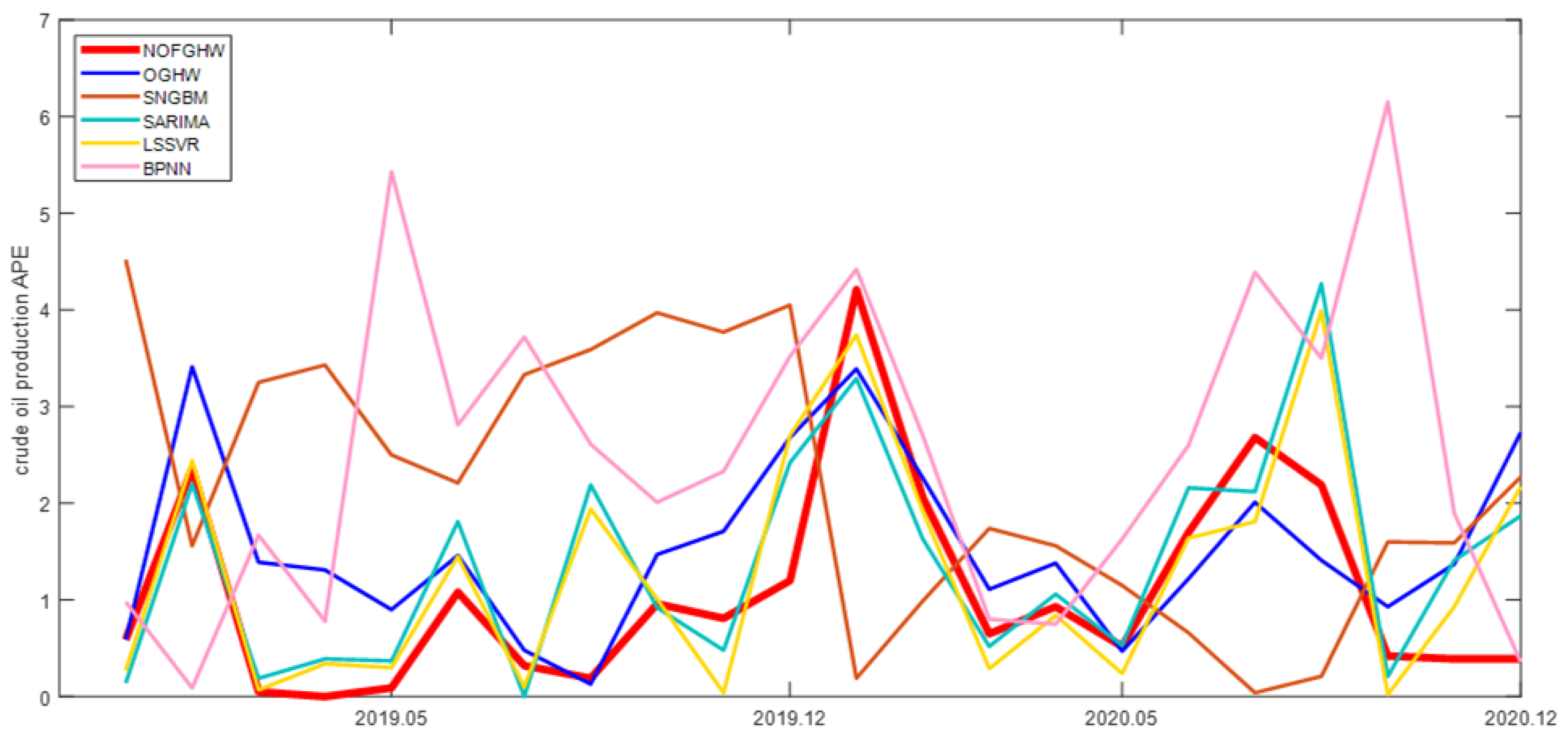
Table 2 lists the APE, MAPE, and RMSE values for the six models. In Table 2, there are two APE values that attract more attention, namely the 2019-M1 point of NOFGHW model and 2019-M8 point of SARIMA model. The APE value at both points is zero, indicating that the prediction error of the two models at these points is zero. The maximum APE value of NOFGHW model in the out-of-sample prediction stage is smaller than that of SARIMA model, indicating that NOFGHW model has better stability (which can also be seen from Figure 5). The APE values of the NOFGHW model in Figure 5 are mostly in a state of small fluctuation and have good stability. It is worth noting that the fluctuation of the SARIMA model and LSSVR model is also small, but the APE values of both models are larger than those of the new model at many points, which means that the prediction effect of the new model is slightly better. The MAPE value in Table 2 is a comprehensive indicator for the simulation and prediction stages. We discovered that three of the four composite indicators of the new model are the smallest among all models. In short, the prediction effect of the new model is better than that of the five comparison models. Although the RMSE value of the new model in the prediction stage is the second smallest, there is no significant difference between it and the minimum value of 34.4965, which does not have a great influence on the prediction results of the model.

In general, the overall performance of the new model is superior to other models both in terms of graph fitting status and evaluation indicators, which verifies the superiority of the new model in dealing with both seasonal and nonlinear sequences and its performance in predicting energy production cases.

3.3.2. Quarterly Industrial Electricity Consumption

Since its reform and opening up, China has vigorously developed its various industries; China has gradually become an industrial power. The development of industry promotes the development of national economy and of all walks of life. Therefore, industry is indispensable to China. In recent years, China’s industrial electricity consumption has risen very fast, and the raw materials used for power generation in China are in constant shortage. In 2020, many places in China have experienced a surge in power curtailment, and many industrial enterprises have implemented power outage mode, which brings inconvenience to the development of industry and further affects China’s economic development and residents’ life. Therefore, scientific and effective prediction of industrial electricity consumption can provide a certain basis for the arrangement of power generation raw materials of relevant departments. In this paper, NOFGHW model and the five comparison models mentioned in Section 3.1 are used for prediction, and the evaluation criteria in Section 2.3 are used to test the model effect, as shown in Figure 6 and Figure 7 and

Table 3. Forecast value of industrial electricity consumption (unit: billion KWH), APE (%), MAPE (%), and RMSE (%).

Quarter	Actual	NOFGHW	APE	OGHW	APE	SNGBM	APE	SARIMA	APE	LSSVR	APE	BPNN	APE
2019-Q1	10,738.00	10,669.57	0.64	10,483.25	2.37	10,433.51	2.84	11,474.12	6.86	11,208.66	4.38	11,719.61	9.14
2019-Q2	11,947.00	11,902.31	0.37	11,671.94	2.30	11,721.35	1.89	13,182.03	10.34	12,167.45	1.85	14,717.78	23.19
2019-Q3	12,528.00	12,474.93	0.42	12,213.86	2.51	12,312.50	1.72	13,600.07	8.56	12,649.03	0.97	12,930.06	3.21
2019-Q4	13,867.00	13,249.82	4.45	12,960.64	6.54	13,169.04	5.03	14,896.65	7.43	13,695.93	1.23	14,299.46	3.12
2020-Q1	9671.00	11,102.61	14.80	10,811.17	11.79	10,801.60	11.69	12,897.81	33.37	12,039.49	24.49	12,741.09	31.75
2020-Q2	12,274.00	12,391.42	0.96	12,034.21	1.95	12,133.89	1.14	14,856.86	21.04	12,803.70	4.32	15,136.20	23.32
2020-Q3	13,066.00	12,990.02	0.58	12,590.03	3.64	12,744.86	2.46	15,305.67	17.14	13,217.02	1.16	13,061.18	0.04
2020-Q4	14,917.00	13,800.14	7.49	13,356.76	10.46	13,630.48	8.62	16,778.35	12.48	14,249.21	4.48	14,567.30	2.34
MAPES			2.5874		2.6093		2.7977		3.6339		3.1896		2.6708
RMSES			400.1221		409.8395		358.7538		477.2389		442.9486		374.5778
MAPEP			3.7143		5.1955		4.4240		14.6505		5.3583		12.0134
RMSEP			680.7043		796.7976		683.1337		1931.3505		913.3109		1827.8879

Note: the maximum APE for each model is bolded.

.

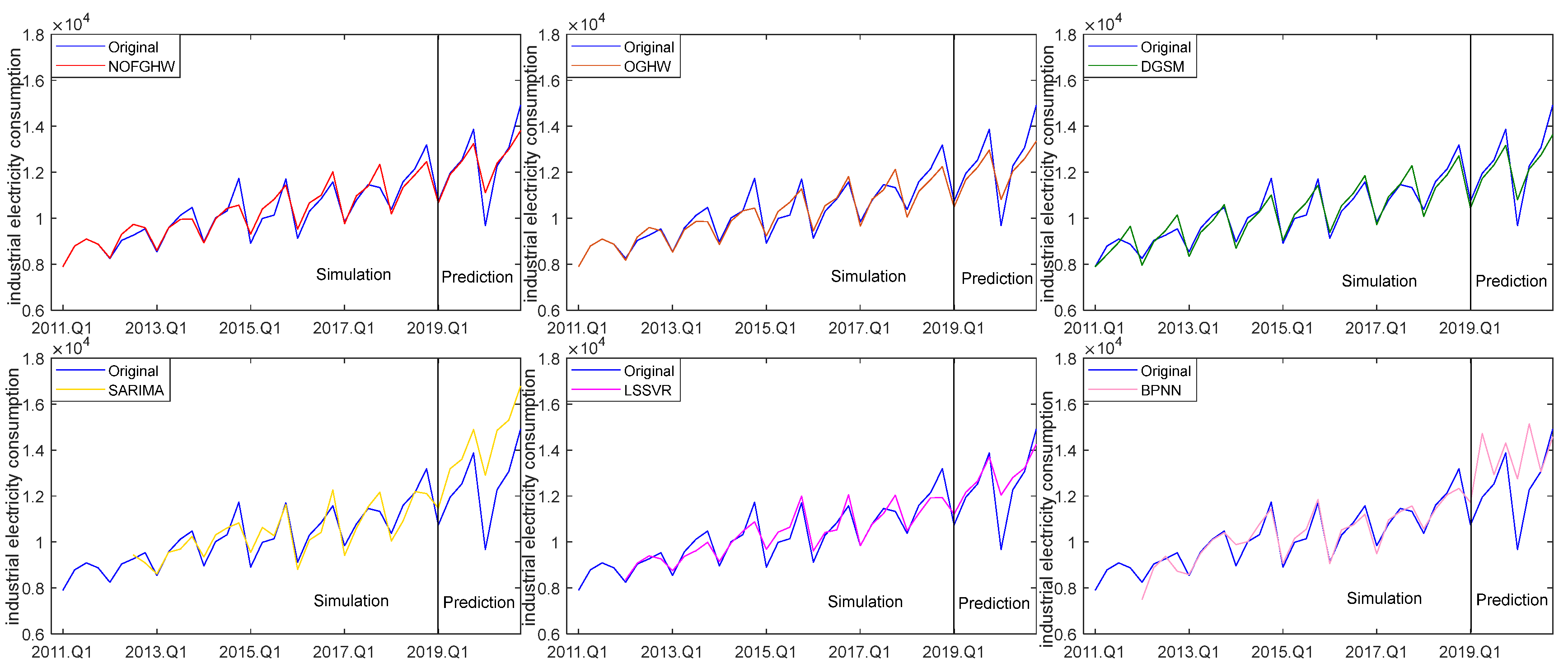
Compared with the case of crude oil production, the quarterly electricity consumption case has fewer sample data and weaker seasonally. Figure 6 intuitively shows the fitting effects of the six models in the simulation and prediction stages. It can be seen from the figure that all six of the models fit the original data series well in the simulation stage, demonstrating that they also have excellent performance in the series with weak seasonality. In the prediction stage, NOFGHW, OGHW, and SNGBM models are closer to the original data sequence than the other three models. Moreover, the NOFGHW model almost completely fits the original data series at several data points later in the first quarter of 2019, while the OGHW and SNGBM models are slightly inferior.

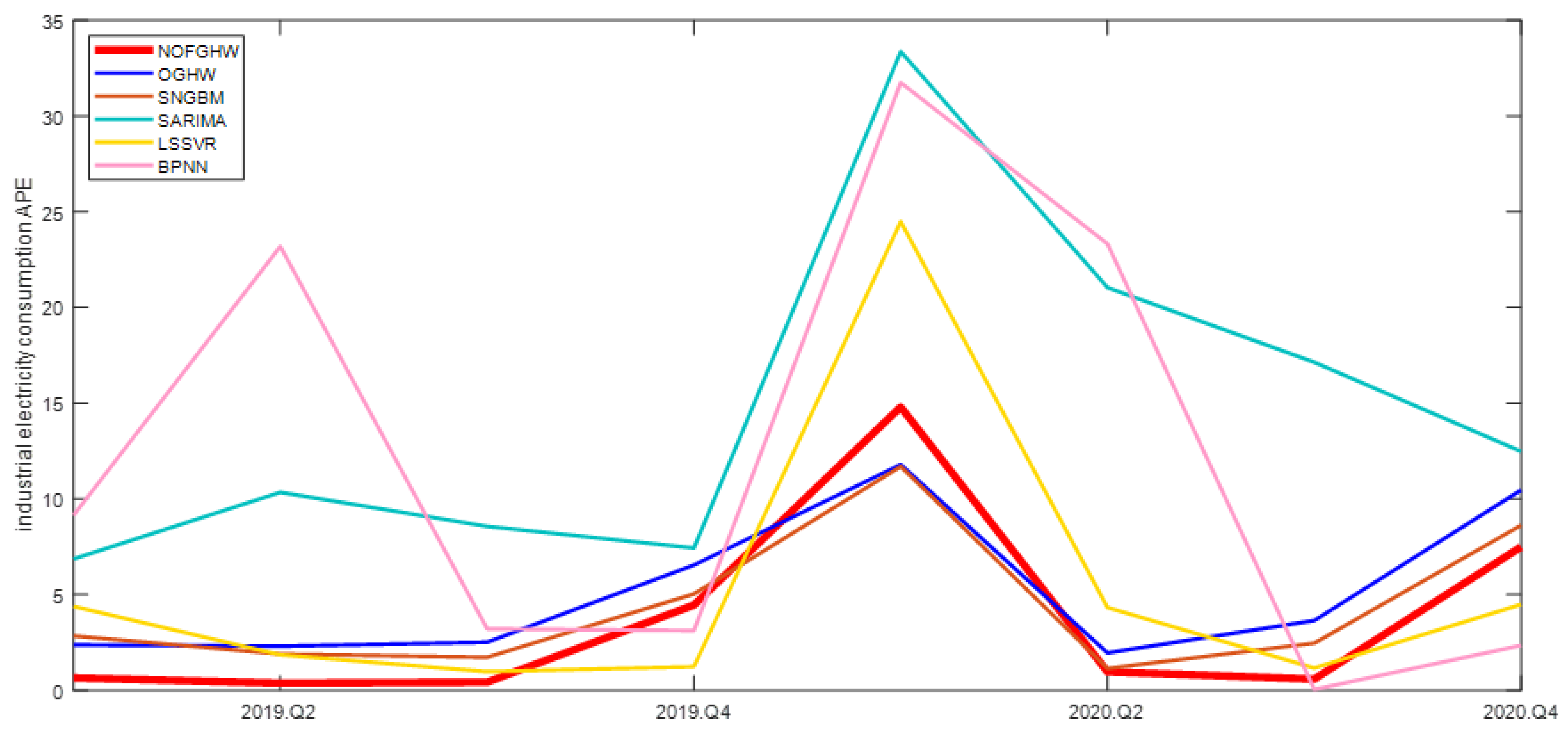
Table 3 lists the APE, MAPE, and RMSE values for the six models. It can be seen from Table 2 that among the eight predicted values of APE, five of the new models are less than one, and one of the LSSVR model and BPNN model are less than one, respectively. This shows that the new model has strong flexibility when dealing with seasonal sequence of different degrees. Figure 7 illustrates this more clearly. The APE value of the NOFGHW model in Figure 7 is usually at a low level, and the effect is the best. The second best is the SNGBM model. SNGBM model is followed by OGHW model, while LSSVR and BPNN models show a large deviation. The last four rows of values in Table 3 are a comprehensive indicator for the evaluation of the model simulation and prediction stages. Among them, the MAPE value in the simulation stage is the second smallest, which is not much different from the minimum 358.7538. However, three indicators in the new model are the smallest among all models, especially the indicators in the prediction stage which have a certain gap compared to other models.

In short, the new model can also play a strong role in energy consumption cases, which verifies the effect of the new model in dealing with different sample sizes and different degrees of seasonality. The model therefore has a certain degree of adaptability.

4. Conclusions and Future Work

In this paper, a new fractional periodic accumulation operator is proposed and introduced into the Holt–Winters model. On this basis, the LBFGS algorithm is applied to optimize the parameters of the model to construct a novel optimized fractional grey Holt–Winters model, namely the NOFGHW model. In order to further verify the effectiveness of the new model, two cases of monthly crude oil production and quarterly industrial electricity consumption are used for empirical analysis, and the remaining five models are selected as comparison models. Finally, the results show that the new model outperforms other comparison models, validating six effects of the new model. Firstly, the new fractional periodic accumulation operator fully preserves the periodic fluctuation of the data after the accumulation. Secondly, the new model can be directly used in the face of seasonal and nonlinear energy time series without using a specific method, which verifies the practicality of the new model. Thirdly, the superiority of the LBFGS algorithm in a quasi-Newton method in dealing with nonlinear sequence is fully verified. Fourthly, the new model can produce good accuracy in different degrees of seasonal sequence. Fifthly, the new model can obtain better results in different cycle energy cases, which verifies the adaptability of the new model. Sixthly, whether it is energy production or energy consumption, the new model can always produce high-precision prediction results. In general, compared with the traditional model, the new model can more carefully analyze the data rules of energy time series, and provides a simpler and more convenient method to deal with the seasonal and nonlinear energy series. By using the new model to predict energy data, it is beneficial to plan future energy market in advance. Then, the relevant departments ensure a balance between supply and demand in the energy market in order to avoid wasting resources.

In this paper, the NOFGHW model is constructed by combining a newfractional periodic accumulation operator, the Holt–Winters model, and the LBFGS algorithm, and the effectiveness, practicability, superiority, and adaptability of the new model in energy prediction are verified. It is worth mentioning that the cases selected in this paper have both seasonal and nonlinear characteristics. However, in reality, not all energy time series have these two characteristics, and may have other more complex characteristics. Therefore, the prediction of energy time series with additional characteristics will be the direction of future research. Furthermore, the question concerning how to use the new model for seasonal and nonlinear time series in other fields and how to apply the new model to other fields is also worth investigating further.

References

- Chen, H.; Li, L.; Lei, Y.L.; Wu, S.; Yan, D.; Dong, Z. Public health effect and its economics loss of PM2.5 pollution from coal consumption in China. Sci. Total Environ. 2020, 732, 138973. [Google Scholar] [CrossRef] [PubMed]
- Zhang, Y.X.; Wang, H.K.; Liang, S.; Xu, M.; Zhang, Q.; Zhao, H.; Bi, J. A dual strategy for controlling energy consumption and air pollution in China’s metropolis of Beijing. Energy 2015, 81, 294–303. [Google Scholar] [CrossRef]
- Xiao, Q.Z.; Gao, M.Y.; Xiao, X.P.; Goh, M. A novel grey Riccati–Bernoulli model and its application for the clean energy consumption prediction. Eng. Appl. Artif. Intell. 2020, 95, 103863. [Google Scholar] [CrossRef]
- Wang, Y.; Nie, R.; Ma, X.; Liu, Z.; Chi, P.; Wu, W.; Guo, B.; Yang, X.; Zhang, L. A novel Hausdorff fractional NGMC(p,n) grey prediction model with Grey Wolf Optimizer and its applications in forecasting energy production and conversion of China. Appl. Math. Model. 2021, 97, 381–397. [Google Scholar] [CrossRef]
- Wang, B.J.; Zhu, C.Q. Research on Trend and Forecast of Coal Prices under Capacity Reduction Based on ARIMA Model. Price Theory Pract. 2017, 5, 73–76. [Google Scholar]
- Liu, K.; Zhang, X. Coal consumption forecast based on fractional ARIMA model. J. Min. Sci. Technol. 2017, 2, 489–496. [Google Scholar]
- Dabral, P.P.; Murry, M.Z. Modelling and Forecasting of Rainfall Time Series Using SARIMA. Environ. Processes 2017, 4, 399–419. [Google Scholar] [CrossRef]
- Sigauke, C.; Chikobvu, D. Prediction of daily peak electricity demand in South Africa using volatility forecasting models. Energy Econ. 2011, 33, 882–888. [Google Scholar] [CrossRef]
- Aasim Singh, S.N.; Mohapatra, A. Repeated wavelet transform based ARIMA model for very short-term wind speed forecasting. Renew. Energy 2019, 136, 758–768. [Google Scholar] [CrossRef]
- Duan, Y.G.; Wang, H.; Wei, M.Q.; Tan, L.; Tao, Y. Application of ARIMA-RTS Optimal Smoothing Algorithm in Gas Well Production Prediction. Petroleum 2021. Available online: https://www.sciencedirect.com/science/article/pii/S240565612100064X#:~:text=ARIMA%2DRTS%20optimal%20smooth%20algorithm%20improves%20the%20prediction%20accuracy%20of,well%20as%20other%20fuels%20output (accessed on 4 February 2022).
- Abbasi, A.; Khalili, K.; Behmanesh, J.; Shirzad, A. Estimation of ARIMA model parameters for drought prediction using the genetic algorithm. Arab. J. Geosci. 2021, 14, 841. [Google Scholar] [CrossRef]
- Zhang, W.Q.; Lin, Z.; Liu, X.L. Short-term offshore wind power forecasting-A hybrid model based on Discrete Wavelet Transform (DWT), Seasonal Autoregressive Integrated Moving Average (SARIMA), and deep-learning-based Long Short-Term Memory (LSTM). Renew. Energy 2022, 185, 611–628. [Google Scholar] [CrossRef]
- Ding, W.; Meng, F.Y. Point and interval forecasting for wind speed based on linear component extraction. Appl. Soft Comput. 2020, 93, 106350. [Google Scholar] [CrossRef]
- Wang, Z.; Wang, F.; Su, S. Solar Irradiance Short-Term Prediction Model Based on BP Neural Network. Energy Procedia 2011, 12, 488–494. [Google Scholar] [CrossRef] [Green Version]
- Wen, L.; Yuan, X.Y. Forecasting the annual household electricity consumption of Chinese residents using the DPSO-BP prediction model. Environ. Sci. Pollut. Res. 2020, 27, 22014–22032. [Google Scholar] [CrossRef] [PubMed]
- Ning, H.; Zhou, W.W. Research on coal price prediction model using the ε-SVR method based on sliding time window. Coal Econ. Res. 2020, 40, 12–18. [Google Scholar]
- Hasanipanah, M.; Shahnazar, A.; Amnieh, H.B.; Armaghani, D.J. Prediction of air-overpressure caused by mine blasting using a new hybrid PSO–SVR model. Eng. Comput. 2017, 33, 23–31. [Google Scholar] [CrossRef]
- Guo, J.; Wang, B.; He, Z.X.; Pan, B.; Du, D.-X.; Huang, W.; Kang, R.-K. A novel method for workpiece deformation prediction by amending initial residual stress based on SVR-GA. Adv. Manuf. 2021, 9, 483–495. [Google Scholar] [CrossRef]
- Tikhamarine, Y.; Souag-Gamane, D.; Kisi, O. A new intelligent method for monthly streamflow prediction: Hybrid wavelet support vector regression based on grey wolf optimizer (WSVR–GWO). Arab. J. Geosci. 2019, 12, 540. [Google Scholar] [CrossRef]
- Hong, W.C. Electric load forecasting by seasonal recurrent SVR (support vector regression) with chaotic artificial bee colony algorithm. Energy 2011, 36, 5568–5578. [Google Scholar] [CrossRef]
- Tikhamarine, Y.; Malik, A.; Pandey, K.; Sammen, S.S.; Souag-Gamane, D.; Heddam, S.; Kisi, O. Monthly evapotranspiration estimation using optimal climatic parameters: Efficacy of hybrid support vector regression integrated with whale optimization algorithm. Environ. Monit. Assess. 2020, 192, 696. [Google Scholar] [CrossRef]
- Wei, M.K.; Ye, W.; Shen, J.; Zhou, H.; Cai, S.R.; Wang, Y.H.; Shen, L. Short-Term Load Forecasting Method Based on Self-Organizing Feature Mapping Neural Network and GA-Least Square SVC Model. Mod. Electr. Power 2021, 38, 17–23. [Google Scholar]
- Khwaja, A.S.; Anpalagan, A.; Naeem, M.; Venkatesh, B. Joint bagged-boosted artificial neural networks: Using ensemble machine learning to improve short-term electricity load forecasting. Electr. Power Syst. Res. 2020, 179, 106080. [Google Scholar] [CrossRef]
- Liu, S.F. Grey System Theory and Its Applications, 5th ed.; Nanjing University of Aeronautics and Astronautics: Nanjing, China, 2010. [Google Scholar]
- Wu, L.F.; Liu, S.F.; Liu, J. GM(1,1) model based on fractional order accumulating method and its stability. Control Decis. 2014, 29, 919–924. [Google Scholar]
- Wu, L.F.; Liu, S.F.; Yao, L.G.; Yan, S.; Liu, D. Grey system model with the fractional order accumulation. Commun. Nonlinear Sci. Numer. Simul. 2013, 18, 1775–1785. [Google Scholar] [CrossRef]
- Wu, L.F.; Liu, S.F.; Yao, L.G.; Xu, R.; Lei, X. Using fractional order accumulation to reduce errors from inverse accumulated generating operator of grey model. Soft Comput. 2015, 19, 483–488. [Google Scholar] [CrossRef]
- Wu, L.F.; Liu, S.F.; Cui, W.; Liu, D.-L.; Yao, T.-X. Non-homogenous discrete grey model with fractional-order accumulation. Neural Comput. Appl. 2014, 25, 1215–1221. [Google Scholar] [CrossRef]
- Zeng, L.; Luo, S.G. A Discrete GM(2,1) Model with Fractional-Order Accumulation and Application. J. Chongqing Norm. Univ. (Nat. Sci.) 2021, 38, 73–80+2. [Google Scholar]
- Jiang, J.M.; Wu, W.Z. Nonlinear grey Bernoulli Model with Fractional-order Opposite-direction Accumulation and Its Application. Math. Pract. Theory 2021, 51, 48–53. [Google Scholar]
- Zhang, A.L.; Bai, L.N.; Han, Y.; Zhao, N. Prediction of Air Quality in Zhengzhou Based On multivariable Fractional Grey Model. J. Saf. Environ. 2021, 1–14. Available online: https://le.cnki.net/kcms/detail/detail.aspx?filename=AQHJ20210728003&dbcode=YJGJ&dbname=YJGJTEMP&v= (accessed on 4 February 2022).
- Wang, Y.; He, X.B.; Zhang, L.; Ma, X.; Wu, W.; Nie, R.; Chi, P.; Zhan, Y. A novel fractional time-delayed grey Bernoulli forecasting model and its application for the energy production and consumption prediction. Eng. Appl. Artif. Intell. 2022, 110, 104683. [Google Scholar] [CrossRef]
- Liu, C.; Lao, T.F.; Wu, W.Z.; Xie, W.; Zhu, H. An optimized nonlinear grey Bernoulli prediction model and its application in natural gas production. Expert Syst. Appl. 2022, 194, 116448. [Google Scholar] [CrossRef]
- Liu, C.; Wu, W.Z.; Xie, W.L.; Zhang, J. Application of a novel fractional grey prediction model with time power term to predict the electricity consumption of India and China. Chaos Solitons Fractals 2020, 141, 110429. [Google Scholar] [CrossRef]
- Ding, S.; Li, R.J. Forecasting the sales and stock of electric vehicles using a novel self-adaptive optimized grey model. Eng. Appl. Artif. Intell. 2021, 100, 104148. [Google Scholar] [CrossRef]
- Wu, W.Z.; Pang, H.D.; Zheng, C.L.; Xie, W.; Liu, C. Predictive analysis of quarterly electricity consumption via a novel seasonal fractional nonhomogeneous discrete grey model: A case of Hubei in China. Energy 2021, 229, 120714. [Google Scholar] [CrossRef]
- Wang, Z.X.; Wang, Z.W.; Li, Q. Forecasting the industrial solar energy consumption using a novel seasonal GM(1,1) model with dynamic seasonal adjustment factors. Energy 2020, 200, 117460. [Google Scholar] [CrossRef]
- Zhou, W.J.; Ding, S. A novel discrete grey seasonal model and its applications. Commun. Nonlinear Sci. Numer. Simul. 2021, 93, 105493. [Google Scholar] [CrossRef]
- Wang, Z.X.; Li, Q.; Pei, L.L. Grey forecasting method of quarterly hydropower production in China based on a data grouping approach. Appl. Math. Model. 2017, 51, 302–316. [Google Scholar] [CrossRef]
- Xia, M.; Wong, W.K. A seasonal discrete grey forecasting model for fashion retailing. Knowl.-Based Syst. 2014, 57, 119–126. [Google Scholar] [CrossRef]
- Zhou, W.J.; Pan, J.; Tao, H.H.; Ding, S.; Chen, L.; Zhao, X. A novel grey seasonal model based on cycle accumulation generation for forecasting energy consumption in China. Comput. Ind. Eng. 2021, 163, 107725. [Google Scholar] [CrossRef]
- Wu, L.F.; Gao, X.H.; Xiao, Y.L.; Liu, S.; Yang, Y. Using grey Holt–Winters model to predict the air quality index for cities in China. Nat. Hazards 2017, 88, 1003–1012. [Google Scholar] [CrossRef]
- Zheng, C.L.; Wu, W.Z.; Xie, W.L.; Li, Q.; Zhang, T. Forecasting the hydroelectricity consumption of China by using a novel unbiased nonlinear grey Bernoulli model. J. Clean. Prod. 2021, 278, 123903. [Google Scholar] [CrossRef]
- Ding, S.; Xu, N.; Ye, J.; Zhou, W.; Zhang, X. Estimating Chinese energy-related CO2 emissions by employing a novel discrete grey prediction model. J. Clean. Prod. 2020, 259, 120793. [Google Scholar] [CrossRef]
- Qian, W.Y.; Sui, A.D. A novel structural adaptive discrete grey prediction model and its application in forecasting renewable energy generation. Expert Syst. Appl. 2021, 186, 115761. [Google Scholar] [CrossRef]
- Ding, S.; Li, R.J.; Wu, S.; Zhou, W. Application of a novel structure-adaptative grey model with adjustable time power item for nuclear energy consumption forecasting. Appl. Energy 2021, 298, 117114. [Google Scholar] [CrossRef]
- Ding, S.; Tao, Z.; Zhang, H.H.; Li, Y. Forecasting nuclear energy consumption in China and America: An optimized structure-adaptative grey model. Energy 2022, 239, 121928. [Google Scholar] [CrossRef]
- Zhou, W.J.; Wu, X.L.; Ding, S.; Chen, Y. Predictive analysis of the air quality indicators in the Yangtze River Delta in China: An application of a novel seasonal grey model. Sci. Total Environ. 2020, 748, 141428. [Google Scholar] [CrossRef] [PubMed]
- Zhou, W.J.; Cheng, Y.K.; Ding, S.; Chen, L.; Li, R. A grey seasonal least square support vector regression model for time series forecasting. ISA Trans. 2021, 114, 82–98. [Google Scholar] [CrossRef]
Figure 1.
The number of works in the literature on energy prediction in the past 10 years.
Figure 2.
Construction of the NOFGHW model.
Figure 3.
Flow chart of NOFGHW model.
Figure 4.
Simulation and forecast graphs of six models for monthly crude oil production cases (Unit: 10,000 tons).
Figure 5.
APE values of monthly crude oil production in the out-of-sample prediction stage of the six models.
Figure 6.
Simulation and forecast of six models of industrial electricity consumption in the quarter (unit: billion KWH).
Figure 7.
APE values of the quarterly industrial electricity consumption in the out-of-sample prediction stage of the six models.