Valuing Ecosystem Services for Agricultural TFP: A Review of Best Practices, Challenges, and Recommendations

Abstract

This paper provides a brief overview of methods to incorporate ecosystem service values into measures of agricultural total factor productivity (TFP), both in theory and in practice. This includes a review of the academic literature, a summary of related economic index theory, and a comparison of agency guidelines. We consider areas of consensus between the agencies and the research literature, as well as open debates surrounding the implementation of a standardized ecosystem accounting framework to integrate with existing TFP measures. This helps to bridge the gap between theoretical approaches to measurement and valuation in the research literature and their implementation in practice by national accounting agencies. Better connecting theory to practice also serves to highlight common challenges in the field, including questions of definition, scope, and scale for ecosystem services, as well as data collection and dissemination. We end with a summary of recommendations for moving forward.

1. Introduction

Perhaps more than any other economic sector, agriculture and the environment are intimately linked. Natural resources, including soil and water, serve as key inputs into agricultural production. In turn, agricultural production affects these vital resources, both in terms of scarcity and quality, as well as the climate governing their function. Globally, agricultural production remains a leading contributor to both soil and water degradation and greenhouse gas emissions. At the same time, population growth and economic development exert ever-increasing pressure to increase production in order to meet global food demands. This highlights the need to better understand the role of the environment in agricultural production, better assess the potential for growth, and better account for both resource stock and quality on a global scale.

The United Nations (UN) Millennium Ecosystem Services Assessment (MA) defines ecosystem services as the benefits people obtain from ecosystems. These include provisioning services such as food and water; regulating services such as regulation of floods, drought, land degradation, and disease; supporting services such as soil formation and nutrient cycling; and cultural services such as recreational, spiritual, religious, and other nonmaterial benefits [1]. Agriculture and ecosystem services are closely intertwined, giving rise to the term “agro-ecosystem” to denote the complex relationships between agricultural production and surrounding ecosystems. While agriculture often benefits from provisioning and regulating services, production can also affect the quality and quantity of these services, in both sustaining and degrading ways.

Total Factor Productivity (TFP) provides a general framework for modeling agricultural production and constructing aggregate index measures to allow for the multilateral assessment of agricultural productivity. Standard agricultural TFP measures the growth in total marketed agricultural output relative to the growth in total marketed input use, constructed as a ratio, where TFP values greater than one indicate overall gains to productivity. Standard TFP measures thus exclude any non-marketed natural resources and environmental effects.

We examine recent efforts to adapt standard TFP measures to include ecosystem service values, both in theory and in practice. This includes a review of the academic literature, as well as a comparison of current national and international statistics agency guidelines. The paper proceeds as follows. In the next section, we overview the theory underlying standard TFP measures and its adaptation to incorporate environmental measures. We then review recent advances in the literature, focusing on questions of measurement, aggregation, and valuation. Next, we connect these advances to the current guidelines practiced by a number of Organization for Economic Development and Cooperation (OECD) member countries and the UN. This leads to a discussion of data requirements for the successful implementation of both the theory and guidelines and extant data needs. We consider areas of consensus, both between the literature and guidelines, and between the statistical agencies, as well as open debates for future research. We conclude with a summary of recommendations for moving forward.

2. Modeling Agricultural TFP

2.1. The TFP Concept

Total factor productivity (TFP), also termed multifactor productivity (MFP), relates total output quantity to total input quantity to provide an aggregate measure of economic performance. The TFP concept can be applied at different levels of economic production, from individual producers at the micro level, to the industry/sectoral level, to the national economy as a whole. Increasing TFP values result from output growth exceeding input growth, indicating improved economic performance. Economic index theory provides a theoretical framework for constructing TFP indices in practice, including key topics related to measurement and aggregation. We overview these methods below, and then compare their use in practice by leading agricultural research agencies.

2.2. Theoretical Framework for TFP

The OECD Productivity Manual [2] overviews the main types of productivity measures used by the national statistics agencies, emphasizing that the choice of measure depends on both the measurement purpose and data availability. In general, these productivity measures can be constructed as the ratio of an output index to an input index, in either gross or value-added terms. Specialized measures for capital and labor productivity restrict inputs to these respective types, while TFP (or MFP, using the manual terminology) combines capital and labor into a single input quantity index. TFP/MFP accounts that integrate capital (K) and labor (L) inputs with intermediate inputs energy (E), materials (M), and services (S) are often referred to as ”KLEMS" accounts. The OECD guidelines [2] note that this integration makes KLEMS-type accounts the most appropriate measure for assessing technical change (the World KLEMS Initiative hosts a platform for accessing KLEMS-type data sets worldwide, including links to regional networks such as the EU KLEMS and Asia KLEMS, and statistical KLEMS databases published by national statistical institutes. See https://www.worldklems.net/wkhome (accessed on 22 January 2022)).

2.2.1. Economic Index Theory

Economic index theory connects index number formulae to the theoretical assumptions made for economic production processes, often termed the production theoretic approach to index numbers. A rich literature now exists in this area, pioneered by [3,4,5,6,7]. The Laspeyres, Paasche, Fisher, and Törnquist indices emerge as the most widely implemented indices under the production theoretic approach. Laspeyres and Paasche indices aggregate quantities using base vs. current period values, respectively. The Fisher index takes the geometric average of the Laspeyres and Paasche indices, while the Törnquist index weights this geometric average by the individual quantity component shares.

In [8], the authors overview these indices for aggregate quantities, letting $x_t\in {\Re }_{+}^M$, $q_t\in {\Re }_{+}^N$, $w_t\in {\Re }_{+}^M$, $p_t\in {\Re }_{+}^N$ denote aggregate inputs, outputs, and their respective prices in time t. Corresponding aggregator functions, $X_t$ and $Q_t$, combine input and output quantities into a single scalar value, so that aggregate productivity in time t, $TF{P}_t=\frac{Q_t}{X_t}$. To measure TFP change from a given base period, time s, to time t, the corresponding TFP index is $TFP{I}_{st}=\frac{TF{P}_t}{TF{P}_s}=\frac{Q{I}_{st}}{X{I}_{st}}$, where $Q{I}_{st}=\frac{Q_t}{Q_s}$ and $X{I}_{st}=\frac{X_t}{X_s}$. Additionally, let $s{h}_{mt}$ denote the cost share of the m-th input and $s{h}_{nt}$ denote the income share of the n-th output. Using this notation, the four indices above can be defined as:

i.

Laspeyeres: $TFP{I}_{st}^{LA}=\frac{p_s^{\prime }{q}_t/p_s^{\prime }{q}_s}{w_s^{\prime }{x}_t/w_s^{\prime }{x}_s}=\frac{Q{I}_{st}^{LA}}{X{I}_{st}^{LA}}$;

ii.

Paasche: $TFP{I}_{st}^{PA}=\frac{p_t^{\prime }{q}_t/p_t^{\prime }{q}_s}{w_t^{\prime }{x}_t/w_t^{\prime }{x}_s}=\frac{Q{I}_{st}^{PA}}{X{I}_{st}^{PA}}$;

iii.

Fisher: $TFP{I}_{st}^{FI}=\frac{{(p_s^{\prime }{q}_t{p}_t^{\prime }{q}_t/p_s^{\prime }{q}_s{p}_t^{\prime }{q}_s)}^{0.5}}{{(w_s^{\prime }{x}_t{w}_t^{\prime }{x}_t/w_s^{\prime }{x}_s{w}_t^{\prime }{x}_s)}^{0.5}}=\frac{{\left(Q{I}_{st}^{LA}Q{I}_{st}^{PA}\right)}^{0.5}}{{\left(X{I}_{st}^{LA}X{I}_{st}^{PA}\right)}^{0.5}}$;

iv.

Törnquist: $TFP{I}_{st}^{TO}=\frac{{\displaystyle \prod _{n=1}^N}{q}_{nt}^{0.5(s{h}_{ns}+s{h}_{nt})}}{{\displaystyle \prod _{m=1}^M}{x}_{mt}^{0.5(s{h}_{ms}+s{h}_{mt})}}$.

The input and output components of the Törnquist index are also commonly defined in log form, giving rise to its alternative name, the translog index. In [9], the authors review each of these indices, including key properties from index theory and their associated decompositions into efficiency, revenue, and cost share changes, and provide an axiomatic framework for choosing the appropriate index in practice. Note that each of the indices incorporate price-based weights for aggregation. As [8] explains, “The intuition behind the use of price-weighted aggregator functions is that we should use weights that reflect the relative importance, or value, of each input or output to the firm”. Efforts to include non-marketed ecosystem values draw on a similar intuition, using non-market valuation methods to estimate their relative values for aggregation (see Section 3).

In [6], the authors call for the use of superlative index numbers, which can be directly derived from or are exact to second-order approximations or flexible aggregators of twice differentiable linear homogeneous functions, including utility and production functions from economic theory. The family of superlative index numbers includes the Törnquist index, which is exact for the translog functional form, and the Fisher ideal index, which is exact for the quadratic functional form. The translog and quadratic forms are commonly used to specify production, cost, revenue, and distance functions.

The Malmquist quantity index [4] is also widely applied to estimate TFP, stemming in part from the seminal work of [10]. The Malmquist index employs Shephard distance functions [11], which measure the feasible radial expansion of outputs for given inputs and the feasible radial contraction of inputs for given outputs. Distance functions thus serve as a measure of relative efficiency for individual production units and provide an estimate of the underlying production technology. As the OECD manual [2] notes, the Malmquist relaxes two strong assumptions made by the four indices above: (i) firms or establishments are economically efficient, and (ii) technologies exhibit global constant returns to scale. Real production processes, including agriculture, likely violate these assumptions to varying degrees.

Distance functions themselves impose no functional form for the technology and do not require price data for aggregation. This second property, in particular, lends well to environmental applications in the absence of market prices for environmental quantities, such as ecosystem services, and there is now a large literature on their use in this area (see Section 3). The Malmquist index can also be related to the Fisher and Törnquist indices in exact representation terms by specifying the composite distance functions in quadratic form for the first case and translog form for the second case. The Malmquist index also allows for a number of economically meaningful decompositions of TFP, most notably into separate measures of efficiency change and technology change [7,10,12], though [8] critiques this decomposition due to the Malmquist’s lack of multiplicative completeness (Ref. [8] defines multiplicative completeness: let $TFPI(x_t,q_t,x_s,q_s)$ denote an index number that compares TFP in period s with TFP in period t using period s as the base. $TFPI(x_t,q_t,x_s,q_s)$ is multiplicatively complete if and only if it can be expressed in the form $TFPI(x_t,q_t,x_s,q_s)=[Q\left(q_t\right)/X\left(x_t\right)]/[Q\left(q_s\right)/X\left(x_s\right)]$ where $Q(.)$ and $X(.)$ are non-negative non-decreasing linearly-homogeneous scalar functions).

One additive indicator analogue, as [8] notes, to the Malmquist is the Luenberger indicator [13], which employs non-radial directional distance functions. The Luenberger does satisfy the completeness property (in differenced rather than ratio form), along with several other desirable index properties [14].

2.2.2. Estimation

Empirical estimation of the indices above can follow one of three general approaches: (i) the growth accounting/index number approach, (ii) production function-based approach, and (iii) productivity and efficiency analysis. Within and across these general approaches, estimation can employ both parametric and nonparametric methods.

The index number or growth accounting method takes a direct approach to estimation, using an industry’s observed change in inputs and outputs, along with prices, to compute TFP. This is the approach taken by OECD, KLEMS, and the U.S. Bureau of Labor Statistics and Bureau of Economic Analysis (BLS-BEA) Integrated Industry-Level Production Account. Separating inputs into capital (K), labor (L), energy (E), materials (M), and services (S), aggregate output growth in time t is modeled as

$$\Delta ln{Q}_t=w_K\Delta ln{K}_t+w_L\Delta L_t+w_E\Delta E_t+w_M\Delta M+t+w_S\Delta S_t+\Delta TFP,$$

(1)

where Q denotes aggregate output, w denotes the income factor share for each respective input, and $\Delta TFP$ represents the share of aggregate output growth unexplained by aggregate input growth. In essence, the growth accounting approach models TFP growth as a residual. The input factor shares serve as weights for aggregation to approximate the production elasticities for each of the input categories. Note, the index number method in (1) relies on constant returns to scale for the production technology, meaning that proportional increases in all inputs result in the same proportional increases in all outputs. OECD [2] notes three additional simplifying assumptions made by the growth accounting approach, which if met (approximately) allow for the construction of TFP indexes based solely on observed price and quantity data. These simplifying assumptions are as follows:

• Production processes can be represented by production or transformation functions at various levels of the economy. Production functions relate maximum producible output to sets of available inputs;
• Producers behave efficiently—i.e., they minimize costs and/or maximize revenues;
• Markets are competitive, and market participants are price-takers who can only adjust quantities but not individually act on market prices.

The remaining estimation methods relax these assumptions to varying degrees. The production function approach employs econometric techniques to estimate production elasticities for inputs, without imposing income shares for aggregation, and not necessarily imposing constant returns to scale. OECD [2] notes several drawbacks, however, for this approach in practice by statistical agencies. These include (i) difficulty in routine updating, due to re-estimation of systems of equations; (ii) difficulty communicating methodologies to a broad audience; and (iii) difficulty releasing timely results due to significant data requirements. These difficulties make the production function approach more appropriate for academic research and case studies. The production function approach is employed by the EU Economic and Financial Affairs Council (ECOFIN) to estimate potential TFP growth. Key references in the literature include [15,16,17,18]. In [19], the authors also provide a comprehensive review focused on the production function approach to productivity.

Productivity and efficiency analysis methods relax the efficiency assumption, allowing for the estimation of both firm-level and aggregate inefficiency in production. This approach employs distance functions to model the production technology at given points in time and construct TFP indexes to decompose productivity into both efficiency change and technology change, in addition to the standard decompositions under efficiency assumptions. Estimation can either employ econometric methods, generally referred to as Stochastic Frontier Analysis (SFA), or nonparametric linear programming methods, known as Data Envelopment Analysis (DEA), though recent efforts to merge the two also exist (Kuosmanen and Johnson, 2010; Parmeter and Zelenyuk, 2019). Both estimation approaches allow for non-constant returns to scale. The literature is vast. For methodological overviews, see Kumbahakar and Lovell (2000) for SFA and Coelli et al. (2005) for DEA. For a recent comprehensive review of both approaches, including theory and application, see Sickles and Zelenyuk (2019).

2.3. Existing Agricultural TFP Indexes

Given the role of agriculture in feeding populations, trade, and the global economy, national statistics agencies and international bodies such as OECD and the UN devote considerable resources to measuring agricultural TFP. More broadly, three international agency manuals guide TFP index construction in practice [20]. The 2009 UN System of National Accounts (SNA) provides a set of internationally accepted standard accounting rules for tracking economic activity in any country, disaggregating the economy into production units and household units, whose income represents their economic production. The OECD Productivity Manual [2] provides a comprehensive theoretical framework for measurement to facilitate international comparisons at different levels of aggregation. At the sectoral level, the Eurostat (European Commission, 2000) manual for the Economic Accounts for Agriculture and Forestry [21] applies the SNA classification guidelines to the sectoral accounts. In addition to these, the United States Department of Agriculture (USDA) Economic Research Service (ERS) Agricultural Productivity Accounts have served as a leading model for measuring agricultural productivity [20].

Beginning with the output component to TFP, [22] overviews and compares the leading agency guidelines for measuring gross output for agricultural product accounts, focusing on the SNA [23] and OECD [2] guidelines, as well as the European Commission (EC) Economic Accounts for Agriculture (EEA) [21], the ERS TFP program [20], and the UN Food and Agriculture Organization (FAO) Global Strategy to improve Agricultural and Rural Statistics manual [24]. Key insights for output quantity include the following: first, only the FAO recommends using the value-added (as opposed to gross) approach to measure production output. ERS addresses the two as complements at the industry level, but states that gross measures are more appropriate because they do not impose the arbitrary and generally unsupported assumption of weak separability of the underlying production function between labor and capital provided by the sector and inputs provided by other sectors. The EEA excludes production for intermediate consumption, but includes intermediate production. The EEA also excludes on-farm losses, referring to the resulting measure as usable gross output. Areas left unaddressed by all of the manuals include commodity specificity (i.e., level of detail and disaggregation of commodity outputs) and the need for supply–demand balance (i.e., the adding up of output quantities produced vs. output quantities used). The manuals largely conflict on the treatment of intrasectoral use, which serves as an intermediate input, but must often be estimated from inventory data.

For output prices, there is a consensus regarding the use of basic unit prices, including unit subsidies, to value gross output. Furthermore, purchaser prices may be used in the absence of basic prices as a way to derive the basic unit price or, in the presence of basic price data of unknown quality, as a way to validate basic unit prices. Related to this, there is little consensus on which subsidy policies to include in basic prices; for instance, product subsidies vs. practice subsidies. For intermediate inputs and intrasectoral use, data availability and quality of inventory tracking pose a shared obstacle across agencies.

Turning to the input component of TFP, one important aspect across existing indices concerns distinguishing between the flow of services and the stock of input variables (Fuglie et al., 2016). For example, services flowing from agricultural land and capital should be reflected in their rental rates, which are often more readily available for land than for capital. This distinction between service flows and stock values is also relevant for ecosystem service accounting (see Section 3). In both cases, it is the flow of services in each year that serves as the actual input into the production process.

Another aspect, relevant to both the input and output components, concerns qualitative adjustments to index values [25]. For instance, while some of the accounting agencies do include agricultural land area as a capital input for agricultural TFP, they do not account for changing land quality over time (e.g., loss of fertility or increased erosion), with the exception (at least to some extent) of ERS [26]. In [25], the authors suggest two approaches to account for quality. The first is to disaggregate the input into qualitative classes; for instance, separate land quality categories, and then track changes in the composition of the input classes over time [27]. Alternatively, input prices should reflect qualitative attributes in competitive markets, so that as the distribution of these characteristics change over time, prices could be used to normalize the input to a constant quality unit [28]. Both approaches are consistent with the OECD guidelines to measure production in constant quality units. In [20], the authors also address quality adjustments, presenting a simple model of production with quality change to illustrate the identification issues in disentangling changes to output quality and changes to TFP. While changes to input quality simply move production along a given output frontier, changes to output quality shift the frontier, along with changes to TFP. Again, there are direct parallels for ecosystem service accounting, where often the services contributing to agricultural production depend on ecosystem condition. We consider this aspect more for ecosystem services in the next section.

3. Incorporating the Environment

3.1. Ecosystem Services

3.1.1. Classification and Accounting Methods

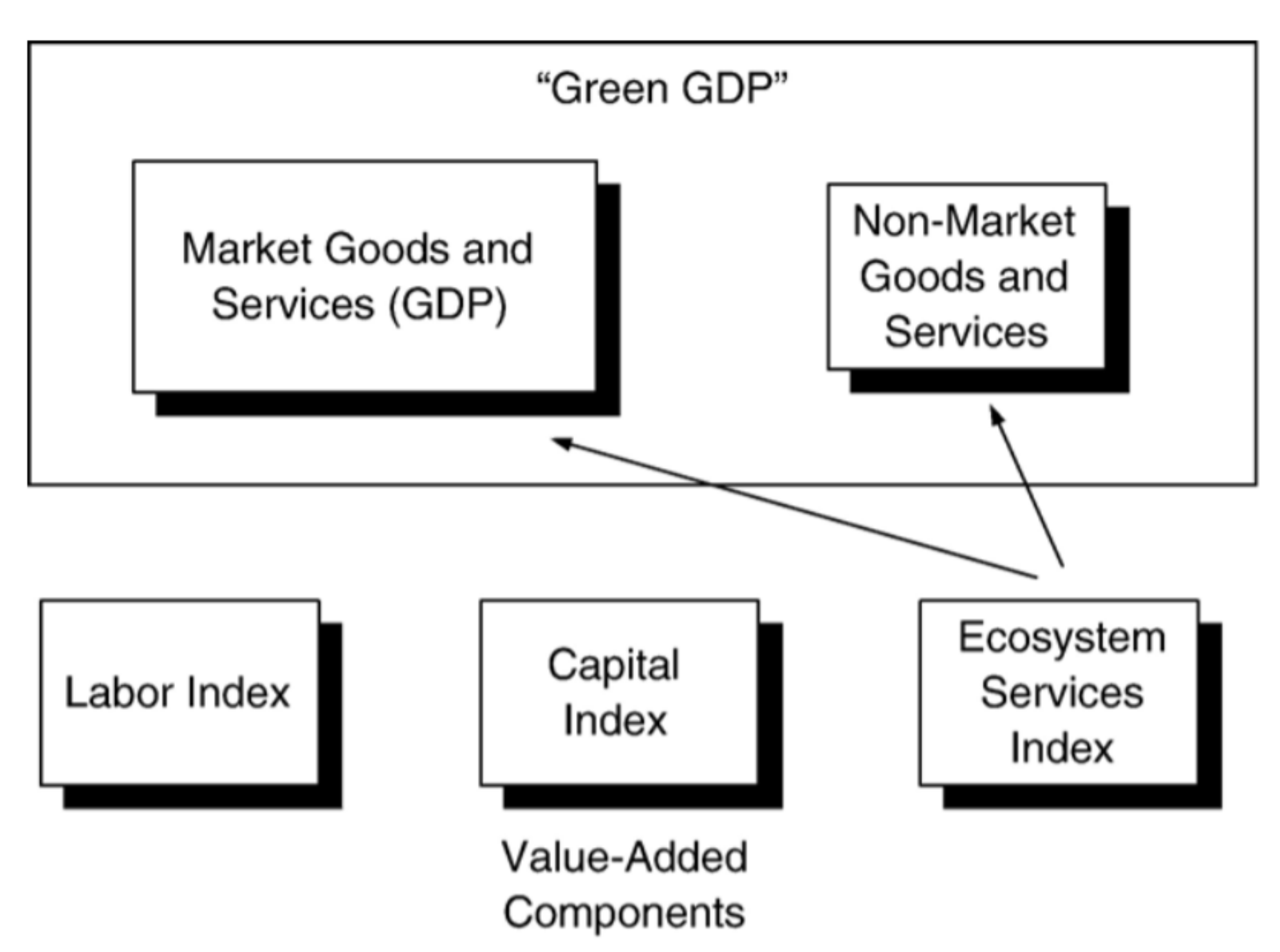
The MA [1] classification of ecosystem services into three types (provisioning, regulating, and cultural) provides a starting point for identifying the different types of services related to agro-ecosystems. Ref. [29] develop a standardized approach to measurement, drawing on gross domestic product (GDP) accounting methods to restrict analysis to final ecosystem services. They define final ecosystem services as components of nature directly enjoyed, consumed, or used to yield human well-being. They offer two alternative approaches to measurement, constructing a “Green GDP" based on final welfare benefit and an ecosystem service index (ESI) based on final contributions to both welfare and the ecosystem. Figure 1 illustrates these two approaches to measurement.

Measurement under either approach requires first defining standardized units of account and then specifying appropriate weights for aggregation, in the absence of market prices. To standardize the unit of account, ref. [29] defines services in terms of final end product components or characteristics rather than also including intermediate functions and processes. They offer as an example the conventional GDP corollary for manufacturing, where only the final manufactured good, and not the intermediate manufacturing process, would be included. They further distinguish quantities in terms of total (stock) and changes to the total (flows), which allows them to draw on duality relationships in production theory to value individual ecosystem services in terms of their marginal product as inputs into final marketed goods, such as agricultural products. When the ecosystem service is itself the final consumed product or an input into another nonmarketed benefit (e.g., the recreation benefit from bird-watching), then willingness to pay estimates from the non-market valuation literature could be used as value weights for aggregation.

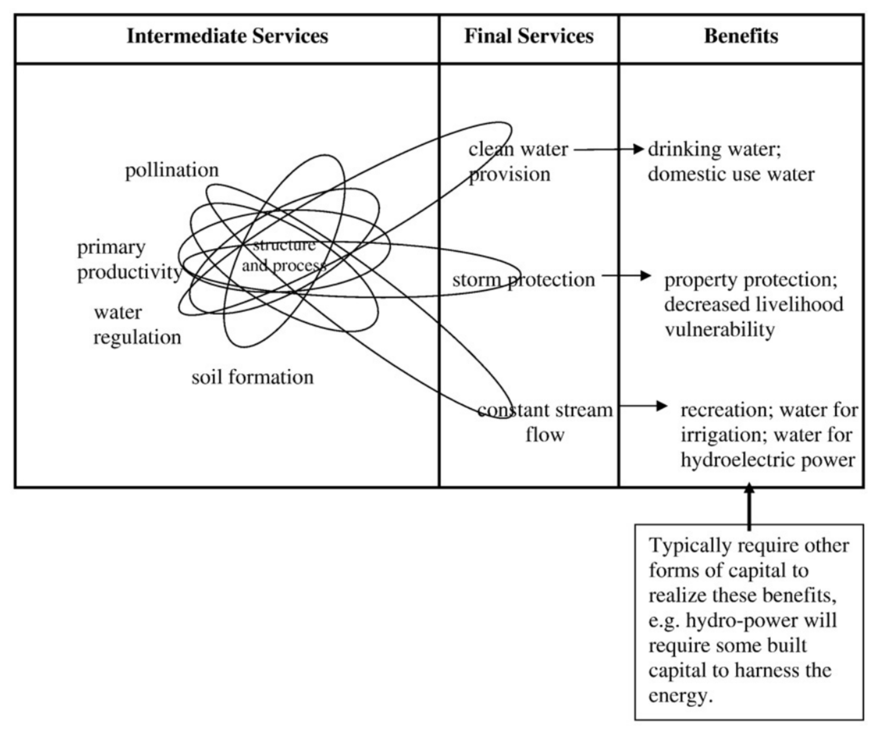
A number of studies (900+ citations) build on the framework from [29]. Notably, [30] maintains a similar focus on ecological components as quantity outputs, but argue that classification should also depend on the decision context or motivation for which ecosystem services are being considered. Relevant decision contexts include education, benefit–cost analysis, landscape management, and public policy. They also argue that the supporting structures and processes, considered intermediate inputs by [29], should themselves be considered as services if (and only if) they benefit humans. Figure 2 conceptually links ecosystem structure, processes, services, and benefits to humans.

Related to the importance of the relevant decision context, ref. [31] argues for multiple classification systems. In [32], the authors review the evolution of ecosystem service definitions, identifying four main approaches to classification: Natural Science [33,34,35], Ecology–Economics Hybrid [36,37], Economics [29], and Generalized or Public Policy [1,38].

Moving from definition and classification to application, much of the literature pertains to specific types of ecosystem services. Examples with implications for agriculture include hydrologic services [39,40], soils [41], estuarine and coastal services [42], and pollination [43].

In practice, government agency guidelines also shape current ecosystem service accounting. Examples include the Final Ecosystem Goods and Services Classification System (FEGS) and National Ecosystem Services Classification System (NESCS) developed by the US Environmental Protection Agency (EPA); The Economics of Ecosystems and Biodiversity project (TEEB), developed by the European Commission; and The Common International Classification of Ecosystem Services (CICES), developed by the European Environmental Agency (EEA) and now contributing to the broader System of Environmental–Economic Accounting for Agriculture, Forestry, and Fisheries (SEEA AFF) led by the United Nations Statistical Division (UNSD).

3.1.2. Challenges

One basic challenge to accounting for ecosystem services lies in reconciling the different definition and classification systems used in the literature and in practice. In [44], the authors summarize and compare the main classification systems from both the literature and agency guidelines, noting that they share more in common than in difference on key points. This suggests some progress towards convergence to a common definition and classification system that could be applied for global accounting.

Valuation poses another basic challenge to accounting. This includes the determination of which values to include and which methods to use. Types of value include both economic value to humans and non-economic values related to principles of fairness and equity, as well as ecological value [45]. Restricting to economic values, arguably most relevant to agricultural TFP, valuation methods include both consumption-oriented stated and revealed preference approaches [46], as well as production-oriented shadow price [47] and production-function approaches [48].

The SEEA AFF White Cover [49] lists a number of general accounting issues in practice. These include defining product scope (e.g., livestock rearing vs. slaughter); treatment of intra-unit flows (e.g., saving seed for future crops); treatment of own-account production (e.g., subsistence farming/fishing, land improvements); treatment of joint products (e.g., sugarcane for sugar and bio-energy); treatment of secondary production (e.g., agro-tourism); treatment of natural and cultivated biological resources (e.g., distinguishing products generated by natural processes from products generated by human activities); treatment of inventories, losses and waste (e.g., discarded fisheries catch, food spoilage, water and energy use inefficiency); and issues concerning measurement and aggregation (e.g., use of monetary aggregates in place of physical quantities to represent agricultural and biological processes).

Addressing the issues listed above requires the collection of detailed data at varying spatial scales and points along the supply chain, which often may not be feasible. Thus, data collection poses another important challenge to environmental accounting. Current guidelines rely more on aggregate environmental indicators for environmental accounting. For SEEA AFF, these include both descriptive statistics on resource use (e.g., total crop irrigation, share of land in crops), environmental assets in either physical or monetary terms (e.g., size vs. value of resource stock), and environmental ratio indicators that relate environmental resources to some form of economic activity (e.g., crop yield per hectare of land). The environmental ratio indicators can also be used to measure decoupling by relating undesirable emissions or energy use to economic activity (e.g., the ratio of greenhouse gas emissions to GDP).

The measurement of quality vs. quantity poses a related challenge to environmental accounting. For agriculture in particular, both the OECD and FAO Statistics (FAOSTAT) agri-environmental indicators databases mainly include quantitative measures of natural assets for accounting purposes, with qualitative measures largely restricted to management practices, such as tillage and fertilizer or pesticide use. In contrast to direct measures of physical quantities for resource stocks and flows, accounting for quality often relies on various environmental indicators to indirectly measure ecosystem function. The SEEA Experimental Ecosystem Accounting (EEA) guidelines consider qualitative measures in terms of condition, where ecosystem condition reflects the overall quality of an ecosystem asset in terms of its characteristics [50].

Condition can be further delineated into measures of the intrinsic state or function of the ecosystem and measures of capacity to generate ecosystem services. In either case, key challenges include the selection of appropriate indicators, aggregation and weighting relative importance, and determining reference or baseline conditions. While indicator selection and reference conditions lie mainly within the purview of the natural sciences, economic index theory addresses methods for aggregation and weighting which can be applied to construct ecosystem condition indexes. Example applications in the literature include water quality indexes [51,52] and soil quality indexes [53].

3.1.3. Opportunities

Recent advances in institutional coordination, policy design, and integrated modeling offer a number of opportunities for ecosystem service accounting. In addition to the UN MA and SEEA programs, other large scale and/or multinational institutional programs include the UN TEEB program, which primarily focuses on biodiversity; the World Bank-led Wealth Accounting and Valuation of Ecosystem Services (WAVES) program; The Natural Capital Project (NatCap), which partners Stanford University, University of Minnesota, The Nature Conservancy, and the World Wildlife Fund; and the UN Intergovernmental Science-Policy Platform on Biodiversity and Ecosystem Services (IPBES), created to support environmental decision making for 126 member countries [44]. Efforts to improve data collection, indicator selection, and standardize measurement and accounting systems for international comparison and assessment cross-cut these large-scale collaborations.

Integrated modeling links natural science-based biophysical models of ecosystem function to social science-based models of related human behavior for decision support. Computational advances, including parallel computing and genetic algorithm solution techniques, allow for more explicit modeling of complex interactions between ecosystems and human activities. Integrated agri-environmental models are now widely use, both in theory and in practice, for policy design and management [54]. Integrated frameworks can be used to simulate both quantitative changes to resource use, as well as qualitative changes in resource condition, resulting from human response to changing market prices and policy incentives. Integrated frameworks can also be used to model tradeoffs between ecosystems and economic activities, and estimate values for ecosystem effects. The NatCap Integrated Valuation of Ecosystem Services and Tradeoffs (InVEST) model serves as one large-scale example of this integrated framework in practice, with application specifically to ecosystem services. In addition to simulating alternative likely economic and environmental scenarios, integrated frameworks can also be re-calibrated to alternative locations, allowing for analysis at larger geographic scale, and facilitating aggregation to country and cross-country levels.

3.2. Biodiversity

Biodiversity plays a unique role in accounting for ecosystem services, both by serving as an indicator of overall ecosystem condition, and supporting ecosystem service flows. The SEEA EEA framework considers biodiversity at three levels: the diversity of ecosystems, species, and genes. However, practical considerations limit the collection and use of genetic biodiversity measures. The SEEA EEA criteria for ecosystem and species-level biodiversity assessment include the following:

• Appropriate spatial resolution for mapping to individual ecosystem assets and types;
• Temporal relevance for assessing changes in stock or condition over the accounting period;
• A common reference condition for comparison and aggregation purposes;
• The ability to aggregate separate indicators into a composite indicator for overall condition;
• Standardization to allow for comparison over space and time across ecosystem types.

These criteria mainly facilitate spatial/temporal matching and aggregation but speak less to determining the individual metrics. For this aspect, SEEA EEA notes that biodiversity-related policy priorities should guide metric selection. For instance, a policy goal to prevent species loss might guide the inclusion of more threatened and endangered species metrics, while maintaining ecosystem condition might guide the inclusion of more umbrella species metrics. For similar reasons, the UN Environment Program World Conservation Monitoring Centre (UNEP-WCMC) proposes the organization of species metrics into separate accounts for (i) conservation concern, (ii) ecosystem condition and/or functioning, and (iii) ecosystem service delivery [55].

The matter of quantity vs. variation, or abundance vs. richness, also plays a role in biodiversity metric selection, particularly for species-level measures. Again, policy goals and the related ecosystem service of interest should guide this selection. A number of studies in the economics literature develop optimization frameworks for weighing this tradeoff, often termed the Noah’s Ark Problem [56,57,58,59]. SEEA EEA also notes the importance of consulting with ecologists on this aspect of biodiversity metric selection for accounting purposes.

Other challenges include a lack of global data at appropriate spatial/temporal resolution for national level accounting and linking biodiversity indicators to individual ecosystem services for both accounting and valuation. These challenges also present opportunities for future research. Other areas for further research include developing accounts for underlying drivers of biodiversity (e.g., habitat fragmentation patterns or invasive species), better calibration of biophysical models for prorating biodiversity measures to appropriate spatial/temporal scales, and the eventual use of biodiversity accounts for policy analysis.

3.3. Bad Outputs

Finally, undesirable environmental effects, often referred to as bad outputs, play an important role in accounting for ecosystem services. Bad outputs generally take one of two forms: those flowing from the ecosystem to humans, and those flowing from humans to the ecosystem. SEEA EEA terms the first of these ecosystem disservices, listing pests and diseases as examples. The second form, commonly termed negative externalities, includes pollution, land degradation, and biodiversity loss. SEEA EEA notes that in contrast to economics, accounting principles do not include welfare effects of use, but instead record strictly positive flows between producers and consumers. Thus, bad outputs only enter indirectly as changes in ecosystem condition and reduced flows of ecosystem services. The main exception to this is flows of greenhouse gas emissions, which SEEA EEA records directly in the carbon account, both as flows (sequestration and emissions) and changes in the stock of carbon.

SEEA EEA defines ecosystem degradation as the decline in condition of an ecosystem asset as a result of economic or other human activity, which is consistent with the SEEA Central Framework approach to natural resource depletion and the SNA approach to the depreciation of produced assets. Ecosystem degradation can be accounted for either as the net present value (NPV) of the decrease in expected flows of ecosystem services or as the change in the NPV of the ecosystem asset due to changes in capacity, in both cases holding prices constant. In addition to accounting for degradation in monetary terms, degradation can also be measured in physical terms through changes in the ecosystem condition indicators.

Another important aspect to accounting for degradation as part of the SEEA EEA framework, in either physical or monetary terms, concerns allocation to different economic units. As opposed to produced assets, ecosystem assets are often not single user/owner, meaning that the economic unit responsible for the degradation may be different from the economic unit affected by the degradation. For instance, the harmful effects of water pollution from agricultural production may be borne by fisheries downstream. Ecosystem complexity further complicates allocation for accounting purposes, as degradation can lead to reductions for multiple ecosystem services, flowing to multiple users.

Current practices are also moving away from the use of estimated restoration costs to value ecosystem degradation, as these values do not represent actual changes in the value of associated ecosystem services or actual payments made in a revealed preferences context. The restoration cost approach is also inconsistent with standard accounting methods for the depreciation of produced assets, which do not consider returning the asset to its original condition. SEEA EEA poses an alternative way to incorporate restoration costs, to instead use the change in estimated restoration costs from beginning to end of the accounting period as an indicator for the cost of a change in condition. Another alternative more consistent with depreciation for produced assets would be to consider the cost of constructing the ecosystem to its current condition.

The literature on accounting for bad outputs considers production at different levels of aggregation, from firm-level to industry/sector-level, to national economy-wide. At the firm and industry/sector-level, much of the focus lies in estimating the pollution-generating technology (PGT) for environmentally adjusted efficiency and productivity analysis. Important theoretical contributions include [14,60,61,62,63,64,65,66]. Recent reviews outlining PGT estimation in practice include [67,68].

The green accounting literature addresses national economy-wide adjustments for bad outputs. In [69], the authors compile early work sponsored by the U.S. BEA Panel on Integrated Environmental Accounting, mainly to incorporate positive-valued environmental goods and resource assets into the national accounts. In [70], the authors use the term externality disaggregation to refer to the reallocation of pollution damage costs and transfer payments between the pollution-generating sector and other affected sectors. In [71], the authors apply this disaggregation approach to U.S. air pollution, using an integrated assessment model to estimate source-specific emissions and marginal damage costs, which they then use to calculate gross annual damages (GAD). In [72], the authors build on this integrated assessment approach to estimate gross damages at both the industry and sector level, developing a framework to incorporate external damages into the national accounts. In [73], the authors address dynamic pollution price effects for the national accounts by computing a set of Paasche, Laspeyres, Fisher, and Törnquist price index numbers for air pollutants. In [74], the authors provide a recent extension of the integrated assessment–disaggregation framework using updated damage cost estimates. This framework has yet to be implemented in practice for the U.S. national accounts.

4. Connecting Ecosystem Accounting to Agricultural TFP in Practice

4.1. SEEA EEA

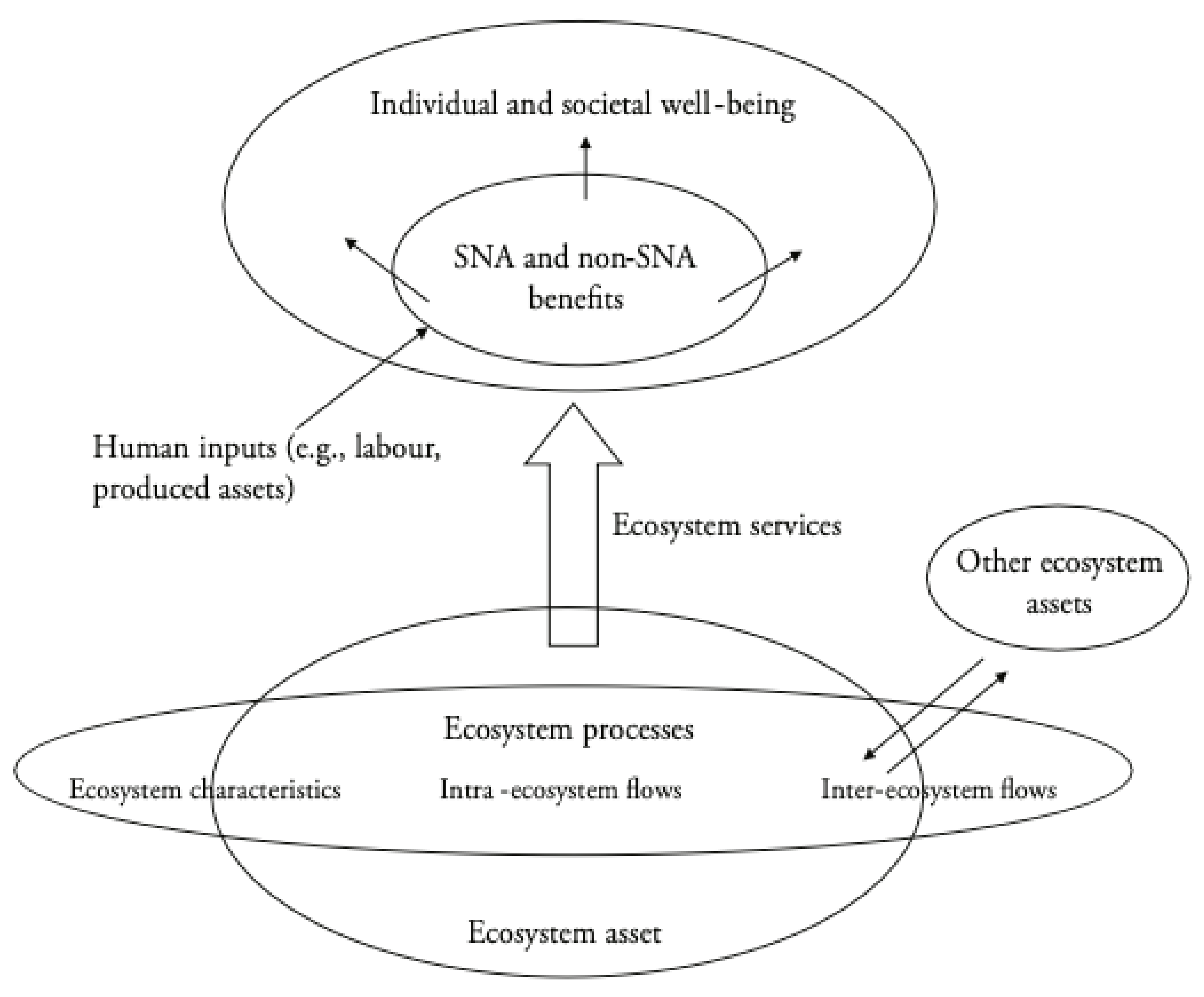
The SEEA EEA provides the leading framework in current practice for incorporating ecosystem accounting into aggregate measures of TFP. In [26], the authors overview the framework, illustrated in Figure 3 below, emphasizing its importance: the SEEA EEA represents a synthesis of approaches to the measurement of ecosystems designed to enable integration with standard national accounting concepts and measurement boundaries.

In this framework, ecosystems (considered assets) generate ecosystem services, which along with human inputs (labor and produced assets) are used to produce benefits to society. These benefits include the goods and services measured by SNA, as well as other social benefits. In [26], the authors highlight the analogous role of ecosystem services to produced capital: the conceptual basis for the extension lies in recognizing that the flows of ecosystem services from agricultural land (in line with the flow of ecosystem services from ecosystem assets in Figure 1) are directly analogous, in accounting terms, to the capital services that flow from produced capital and which are already included in the standard growth accounting MFP measures. Relevant analogues include the use of produced capital depreciation methods for natural resource depletion in the SEEA EEA framework [76], theoretical connections to wealth accounting [77], and the use of produced capital growth accounting methods for natural capital [78].

Obst (2019) distills practical implementation of the SEEA EEA framework to five key steps in order to incorporate ecosystem services into current SNA practices for constructing environmentally adjusted agricultural TFP measures:

• Delineate spatial areas. For agriculture, a spatial area unit of analysis could be single farm or a farming region with similar ecosystem characteristics;
• Measure condition of the ecosystem. The SEEA EEA asset accounts record condition in biophysical indicator terms only;
• Measure the flow of ecosystem services. SEEA EEA guidelines are to maintain a supply use account to record services used by economic units included in the national accounts;
• Relate ecosystem services to standard measures of economic activity. Ecosystem services used as inputs (e.g., water for crops), like other intermediate inputs, have zero net effect on GDP. Ecosystem services considered final outputs (e.g., carbon sequestration), should be added to GDP;
• Use exchange values. Physical trade offs require only quantities, while measurement in monetary terms requires price information. The use of valuation estimates is necessary for many non-marketed ecosystem services.

In [79], the ecosystem accounting principles for capital are extended to agricultural TFP, in three main stages.

• Direct use. The agricultural production unit uses the ecosystem as a production input (e.g., water for irrigation, wild pollination of crops, soil nutrients for crop growth);
• Processing of residual flows. The agricultural production unit uses the ecosystem to mitigate waste generated from production activities (e.g., vegetative filter of runoff, soil absorption);
• Generation of positive externalities. Agriculture also produces some environmental benefits (e.g., carbon sequestration, water regulation, cultural).

Importantly, this accounting framework characterizes ecosystem services in terms of inputs and outputs, allowing for integration with standard agricultural TFP accounting methods and a more informed analysis of tradeoffs between agricultural production and the environment.

4.2. Challenges in Practice

With the exception of a few small pilot studies, the SEEA EEA framework has yet to be implemented in practice, due in part to a lack of ecosystem data, as well as consensus in defining and restricting the set of ecosystem services to include.

4.2.1. Data Requirements and Availability

In terms of data and measurement, [26] broadly divides ongoing issues into four categories:

• Spatial units. The level of ecosystem spatial detail must be compatible with production spatial detail for integration and aggregation;
• Ecosystem condition. The condition data must correspond to the relevant biophysical relationships for ecosystem services to agriculture;
• Ecosystem services. The services to agriculture must be defined and directly measured in input–output form;
• Valuation and accounting. Values should reflect market price-based exchange values, as opposed to welfare values, to be consistent with standard growth accounting for TFP.

The [50] guidelines include a Section 5.6 on data sources. The guidelines suggest the involvement of national statistical agencies, some of which already contribute to the national product accounts. These include the following:

• National Statistical Offices: agricultural production (crops and livestock); health statistics (incidence of environmentally-related diseases), population data, tourism data;
• Meteorological Agencies: rainfall, temperature, climate variables;
• Departments of Natural Resources: timber stock and harvest, biomass harvest for energy, water supply and consumption, natural disaster statistics (floods, landslides, storms), land cover (to estimate carbon stock and sequestration), remote sensing (to estimate primary production);
• Water management and related agencies: water stocks and flows, abstraction rates, data from hydrological modeling;
• Departments of Agriculture: crop production, use of inputs in agriculture, erosion potential, biomass harvest;
• Departments of Forestry: forest stock and harvest, growth rates of forests, carbon sequestration;
• Departments of Environment and Parks: iconic species habitats, visitors to natural areas, biodiversity.

Supplementary global data sets include the International Soil Reference and Information Centre (ISRIC) Harmonized World Soil Database (HWSD) and the ISRIC World Inventory of Soil Emissions (WISE) 3.1 soil profile database, global digital elevation models, forest cover from Global Forest Watch, biophysical indicators from the US National Space and Aeronautics Agency (NASA) Moderate Resolution Imaging Spectroradiometer (MODIS), and hydrology data from WaterWorld. Area research institutions may also compile data from conducted studies. Valuation databases include Environmental Valuation Reference Inventory (EVRI), at www.evri.ca (accessed on 22 January 2022) and the Economics of Ecosystems and Biodiversity (TEEB) based Ecosystem Service Valuation Database (ESVD) at http://www.fsd.nl/esp/80763/5/0/50 (accessed on 22 January 2022).

4.2.2. Definition and Classification of Ecosystem Services for Agriculture

The SEEA EEA guidelines highlight the importance of measurement scope and definition for integration of ecosystem services with the SNA production boundaries. This includes distinguishing final services from intermediate services, as with other areas of the national accounts. Classification also requires determining final end users and benefits, which is needed to construct the supply accounts attaching each service flow to a final user. The guidelines provide some examples of linking ecosystem service types (provisioning, regulating, cultural) to final benefits (e.g., harvested timber, crop biomass, climate regulation, cleaner air and water), noting that in some instances benefits could be both final and intermediate. The SEEA EEA approach to classification is largely consistent with the EU CICES, while alternatives include the US EPA classification system for final ecosystem goods and services (FEGS-CS) [80] and the associated National Ecosystem Service Classification System (NESCS) [81]. The SEEA EEA guidelines note that these alternatives can be seen as complements to one another, as both include hierarchical structures for ecosystem types, uses, and benefits.

4.2.3. Recommendations

The SEEA EEA framework includes a detailed reporting of technical recommendations [79], a number of which are directly relevant to agricultural TFP.

• Establish national spatial data infrastructure (NSDI). Central to these is the need for each country to develop a national spatial data infrastructure (NSDI). The NSDI is critical both for delineating ecosystem spatial areas, but also for connecting these ecosystem areas to land use and other related agricultural production activities. In many cases, much of the work to establish an NSDI has already been done by various government agencies, as well as nongovernmental organizations (NGOs). This highlights the need for cross-agency coordination, as well as public/private data sharing agreements.
• Begin with ecosystem extent. A basic first step, before considering qualitative measures of condition, is to account for total areas for each ecosystem type (e.g., wetlands, grasslands, forest). Ecosystem extent, or land cover maps should be consistent in level of spatial detail with data on land use, to account for ecosystem use. Ecosystem accounting should use the NSDI to integrate ecosystem extent with land use, as well as soil, hydrology, and protected area data.
• Measure ecosystem condition relative to standard reference condition. This facilitates aggregation and comparison and is often more meaningful than raw condition indicator values. The use of the standard reference condition approach also facilitates the comparison of condition across ecosystem types.
• Measure condition by ecosystem type. This builds on the delineation of ecosystem type for extent measures. The measure for each type should use a specified set of indicators that can be replicated across locations. This calls for parsimony in selecting the set of relevant indicators to capture the main aspects of condition, and should draw on scientific expertise.
• Begin with a limited set of ecosystem services. Rather than attempting to capture everything, start with the services which can be readily quantified and connected to agricultural production. In many cases, beginning with soil and water ecosystem services would be most relevant for agriculture, as well as readily measured. Incorporating additional services can then build on the same framework for incorporating these initial services.
• Make use of biophysical models for data. Biophysical process models are well developed and widely used to combine collected observed data and to estimate remaining data for measures of condition and extent. These models are generally spatially explicit, which also allows for integration with land use and agricultural practices. It is important to make transparent the model methods and results in any reporting of accounts using model data.
• Valuation estimates should be exchange values. Values should reflect the monetary value of the contribution of the ecosystem service to economic production and consumption values. The value used for accounting purposes should not be considered a comprehensive or total value of the ecosystem.
• No single valuation method always applies. The valuation approach employed should depend on whether the ecosystem service contributes to a marketed good already included in the national accounts, such as agricultural production, or non-marketed public benefit such as cultural or aesthetic values. Allowing for a variety of valuation methods expands the potential for different types of ecosystem services to be included. It is important to make transparent the given valuation method assumptions and limitations, employing the state of the art from the valuation literature.
• Begin with land and water accounts. Much of the data and methods are generally in place for both land and water accounts. Land accounts also then would serve as an input or foundation for spatial delineation of ecosystems and for integrating ecosystem services with related land use and other agricultural production activities. Water resource accounts should integrate information on groundwater and atmospheric water.
• Measure carbon stocks and flows at national level. All countries should develop national carbon accounts, which can also be disaggregated to sectoral accounts of stocks and flows for carbon.
• Begin with aggregate biodiversity stock. More testing is required to account for causal relationships for species-level changes to biodiversity. This first requires time series data for opening and closing biodiversity levels. Causal drivers of biodiversity should be measured in a supplementary account, once more fully tested. Changes to biodiversity condition should be accounted for separately in the condition accounts.

5. Conclusions

Improving standardized environmental/ecosystem accounting frameworks and insights into interactions between the economy and the environment is crucial. Otherwise, any attempt to develop a comprehensive measure of agricultural TFP to include ecosystem services runs the risk of becoming unusable in practice, particularly for meaningful economic comparisons and aggregation across production units, sectors, regions, and nations. Broadly speaking, both the literature and agencies are progressing towards a more unified framework with this objective in mind. We conclude by considering areas of consensus and open debates moving forward.

One fundamental point of consensus is that environmentally-adjusted measures of TFP should be consistent with current SNA guidelines, so that ecosystem accounts can be integrated with the existing product accounts. Early works in the literature, including [29,70,71], draw on standard accounting methods for GDP to incorporate final environmental outputs, both good and bad. The SEEA EEA framework represents the most fully developed agency-led effort to integrate ecosystem services into the existing product accounts. The national statistical agencies have largely followed suit, including Australia, Canada, the US, the UK, and many EU member states (see [26] for a complete list of countries with activities in support of implementing the SEEA EEA).

Related to this, both the agencies and the literature call for the use of economic valuation methods to estimate monetary values for ecosystem services, for integrating final ecosystem service outputs into the product accounts in the absence of market prices. The distinction between ecosystem stocks and flows, and its analog to produced capital, is also widely shared, as is the recommended use of ecosystem indicators to measure composite condition and to track changes in ecosystem condition from one accounting period to the next, similar to accounting for depreciation or improvements to the capital stock over time.

Beyond these broad areas of consensus, many of the open debates and unresolved research issues surround the underlying details for practical implementation. In [26], these ongoing research issues are separated according to the four components of ecosystem accounting: spatial units, ecosystem condition, ecosystem services, and valuation and accounting. Defining the appropriate spatial scale for analysis and aggregation depends on a number of factors, including ecosystem and production type, as well as region, making the choice of spatial unit less transferable for standard guidelines. While direct service flows, such as water for irrigation, are more readily amenable to integration, measures of ecosystem condition, as well as the biophysical relationships connecting condition to flows, remain less defined. Classification and definition issues for ecosystem services also persist, both in the literature and amongst the agencies. Related to this is the selection of which services to include, particularly for the case of intermediate benefits. The use of economic valuation for accounting purposes by the agencies diverges from the more common use of valuation for estimating welfare effects in the literature. Reconciling this disconnect will likely require the greater use of production-oriented approaches to valuation, to more directly estimate exchange rates between production and the environment. Furthermore, there is some debate on whether to incorporate bad factors, such as pollution, as undesirable outputs or inputs. The productivity analysis literature offers some guidance on this final point.

These unresolved research issues present immediate opportunities for research moving forward, including more formal mathematical modeling of the SEEA EEA framework, biophysical modeling to better measure ecosystem capacity and connect condition to flows, production-oriented approaches to valuation, ecosystem indicator selection, and data collection. Pilot studies may be particularly useful for testing alternative approaches to some of these details on a smaller scale before wider implementation. Advances in remote sensing and computational methods for integrating biophysical–economic modeling, many of which have been developed specifically for agricultural production and associated environmental processes (e.g., soil and hydrology), will aid in many of these efforts, as will the longstanding academic and agency research ties between agriculture, productivity, and environmental and natural resource economics.

A few common themes emerge from the technical recommendations. First, this work should be approached incrementally. Constructing the accounts will require first laying groundwork for spatial analysis, then identifying key initial services, rather than attempting a complete account of all services. Following an incremental approach, each stage of accounting should build and be integrable with the next to allow for the expansion of the accounts to be more detailed and comprehensive over time. Second, the methodology should be transparent and standardized to allow for replication, validation, and comparison both within and across countries, as well as integration into the existing national accounts. However, the framework should also allow some flexibility to accommodate different ecosystem types and different ecosystem uses. Lastly, countries and agencies should work to develop data sharing agreements. Increased data sharing would further standardization and transparency goals, as well as facilitate broader implementation of the accounting framework.

References

- Millennium Ecoysystem Assessment. Ecosystems and Human Well-being: Current State and Trends; Island Press: Washington, DC, USA, 2005. [Google Scholar]
- Organisation for Economic Co-Operation and Development (OECD). Measuring Productivity, Measurement of Aggregate and Industry-level Productivity Growth; Organisation for Economic Co-Operation and Development (OECD): Paris, France, 2001. [Google Scholar]
- Fisher, I. The Making of Index Numbers: A Study of their Varieties, Tests, and Reliability; Houghton Mifflin Company: Boston, MA, USA, 1922. [Google Scholar]
- Malmquist, S. Index numbers and indifference surfaces. Trab. Estat. 1953, 4, 209–242. [Google Scholar] [CrossRef]
- Jorgenson, D.; Griliches, Z. The explanation of productivity change. Rev. Econ. Stud. 1967, 34, 249–283. [Google Scholar] [CrossRef]
- Diewert, W.E. Exact and superlative index numbers. J. Econom. 1976, 4, 115–145. [Google Scholar] [CrossRef]
- Caves, D.W.; Christensen, L.R.; Diewert, W.E. The economic theory of index numbers and the measurement of input, output, and productivity. Econometrica 1982, 50, 1393–1413. [Google Scholar] [CrossRef]
- O’Donnell, C.J. An Aggregate quantity framework for measuring and decomposing productivity change. J. Product. Anal. 2012, 38, 255–272. [Google Scholar] [CrossRef]
- Diewert, W.E.; Nakamura, A.O. Index number concepts, measures and decompositions of productivity growth. J. Product. Anal. 2003, 19, 127–159. [Google Scholar] [CrossRef]
- Färe, R.; Grosskopf, S.; Norris, M.; Zhang, Z. Productivity growth, technical progress, and efficiency change in industrialized countries. Am. Econ. Rev. 1994, 84, 66–83. [Google Scholar]
- Shephard, R. Theory of Cost and Production Functions; Princeton University Press: Princeton, NJ, USA, 1970. [Google Scholar]
- Diewert, W.E. Fisher ideal output, input, and productivity indexes revisited. J. Product. Anal. 1992, 3, 211–248. [Google Scholar] [CrossRef]
- Luenberger, J. Externalities and benefits. J. Math. Econ. 1995, 24, 159–177. [Google Scholar] [CrossRef]
- Chambers, R.; Chung, Y.H.; Färe, R. Benefit and distance functions. J. Econ. Theory 1996, 70, 407–419. [Google Scholar] [CrossRef]
- Olley, G.S.; Pakes, A. The dynamics of productivity in the telecommunications equipment industry. Econometrica 1996, 64, 1263–1297. [Google Scholar] [CrossRef]
- Nadiri, M.I.; Prucha, I. Dynamic factor demand models and productivity analysis. In NBER New Developments in Productivity Analysis; Hulten, C.R., Dean, E.R., Eds.; University of Chicago Press: Chicago, IL, USA, 2001. [Google Scholar]
- Levinsohn, J.; Petrin, A. Estimating production functions using inputs to control for unobservables. Rev. Econ. Stud. 2003, 70, 317–341. [Google Scholar] [CrossRef]
- Aw, B.Y.; Roberts, M.J.; Xu, D.Y. R&D investment, exporting, and productivity dynamics. Am. Econ. Rev. 2011, 101, 1312–1344. [Google Scholar]
- Syverson, C. What determines productivity? J. Econ. Lit. 2011, 49, 326–365. [Google Scholar] [CrossRef] [Green Version]
- Shumway, C.R.; Fraumeni, L.E.; Fulginiti, J.D.; Stefanou, S.E. U.S. Agricultural Productivity: A Review of USDA Economic Research Service Methods. Appl. Econ. Perspect. Policy 2016, 38, 1–29. [Google Scholar] [CrossRef]
- European Commission Office for Official Publications of the European Communities. Manual on Economic Accounts for Agriculture and Forestry; European Commission Office for Official Publications of the European Communities: Luxembourg, 1997. [Google Scholar]
- Cahil, S. What the Manuals Say (or Don’t Say) About Measurement of Gross Output; Background Document; OECD Network on Agricultural Total Factor Productivity and the Environment: Paris, France, 2019. [Google Scholar]
- SNA. System of National Accounts 2008; International Monetary Fund: Washington, DC, USA, 2009. [Google Scholar]
- United Nations Economic and Social Council Statstical Commission. Global Strategy to Improve Agricultural and Rural Statistics Report of the Friends of the Chair on Agricultural Statistics Global Strategy to Improve Agricultural and Rural Statistics Report of the Friends of the Chair on Agricultural Statistics; United Nations Economic and Social Council Statstical Commission: New York, NY, USA, 2010. [Google Scholar]
- Fuglie, K.; Benton, T.; Sheng, Y.; Hardelin, J.; Mondelaers, K.; Laborde, D. Metrics for Sustainable Agricultural Productivity; White Paper, G20 MACS; OECD: Paris, France, 2016. [Google Scholar]
- Obst, C. Incorporating the Environment in Agricultural Productivity: Connecting to Advances in Natural Capital Accounting; Technical Report; OECD Network on Agricultural Total Factor Productivity and the Environment: Paris, France, 2019. [Google Scholar]
- Wang, S.; Heisey, P.; Schimmelpfennig, D.; Ball, E. Agricultural Productivity Growth in the United States: Measurement, Trends, and Drivers; ERS Report ERR-189; United States Department of Agriculture Economic Research Service (USDA ERS): Washington, DC, USA, 2015.
- Ball, E.; Butault, J.; Juan, C.S.; Mora, R. Productivity and international competitiveness of agriculture in the European Union and the United States. In Expert Workshop on Measuring Environmentally Adjusted tfp and Its Determinants; OECD Network on Agricultural Total Factor Productivity and the Environment: Paris, France, 2015. [Google Scholar]
- Boyd, J.; Banzhaf, S. What are ecosystem services? The need for standardized environmental accounting units. Ecol. Econ. 2007, 63, 616–626. [Google Scholar] [CrossRef] [Green Version]
- Fisher, B.; Turner, R.K.; Morling, P. Defining and classifying ecosystem services for decision making. Ecol. Econ. 2009, 68, 643–653. [Google Scholar] [CrossRef] [Green Version]
- Costanza, R. Ecosystem services: Multiple classification systems are needed. Biol. Conserv. 2008, 141, 350–352. [Google Scholar] [CrossRef]
- Danley, B.; Widmark, C. Evaluating conceptual definitions of ecosystem services and their implications. Ecol. Econ. 2016, 126, 132–138. [Google Scholar] [CrossRef]
- Daily, G.C. Introduction: What are ecosystem services? In Nature’s Services: Societal Dependence on Natural Ecosystems; Daily, G.C., Ed.; Island Press: Washington, DC, USA, 1997. [Google Scholar]
- de Groot, R.; Wilson, M.; Boumans, R.M.J. A typology for the classification, descrip- tion and valuation of ecosystem functions, goods and services. Ecol. Econ. 2002, 41, 1–20. [Google Scholar] [CrossRef] [Green Version]
- Wallace, K.J. Classification of ecosystem services: Problems and solutions. Biol. Conserv. 2007, 139, 235–246. [Google Scholar] [CrossRef] [Green Version]
- Fisher, B.; Turner, K.; Zylstra, M.; Brouwer, R.; de Groot, R.; Farber, S.; Ferraro, P.; Green, R.; Hadley, D.; Harlow, J.; et al. Ecosystem services and economic theory: Integration for policy-relevant research. Ecol. Appl. 2008, 18, 2050–2067. [Google Scholar] [CrossRef] [PubMed] [Green Version]
- Haines-Young, R.; Potschin, M. Common International Classification of Ecosystem Services (CICES): Consultation on Version 4; Technical Report Contract Number EEA/IEA/09.003, EEA/IEA; Centre for Environmental Management, University of Nottingham: Nottingham, UK, 2013. [Google Scholar]
- Burke, L.; Ranganathan, J.; Winterbottam, R. Revaluing Ecosystems: Pathways for Scaling Up the Inclusion of Ecosystem Value in Decision Making; Issue Brief; World Resources Institute: Washington, DC, USA, 2015. [Google Scholar]
- Brauman, K.A.; Daily, G.C.; Duarte, T.; Mooney, H.A. The nature and value of ecosystem services: An overview highlighting hydrologic services. Annu. Rev. Environ. Resour. 2007, 32, 67–98. [Google Scholar] [CrossRef]
- Brander, L.; Brouwer, R.; Wagtendonk, A. Economic valuation of regulationg services provided by wetlands in agricultural landscapes: A meta-analysis. Ecol. Eng. 2013, 56, 89–96. [Google Scholar] [CrossRef]
- Dominati, E.; Patterson, M.; Mackay, A. A framework for classifying and quantifying the natural capital and ecosystem services of soils. Ecol. Econ. 2010, 69, 1858–1868. [Google Scholar] [CrossRef]
- Barbier, E.B.; Hacker, S.D.; Kennedy, C.; Koch, E.W.; Stier, A.C.; Silliman, B.R. The value of estuarine and coastal ecosystem services. Ecol. Monogr. 2011, 81, 169–193. [Google Scholar] [CrossRef]
- Gallai, N.; Salles, J.M.; Settele, J.; Vaissière, B.E. Economic Valuation of the vulnerability of world agriculture confronted with pollinator decline. Ecol. Econ. 2009, 68, 810–821. [Google Scholar] [CrossRef]
- Costanza, R.; de Groot, R.; Braat, L.; Kubiszewski, I.; Fioramonti, L.; Sutton, P.; Farber, S.; Grasso, M. Twenty years of ecosystem services: How far have we come and how far do we still need to go? Ecol. Econ. 2017, 28, 1–16. [Google Scholar] [CrossRef]
- Costanza, R.; Folke, C. Valuing Ecosystem Services with Efficiency, Fairness, and Sustainability as Goals. In Nature’s Services: Societal Dependence on Natural Ecosystems; Daily, G.C., Ed.; Island Press: Washington, DC, USA, 1997; pp. 49–69. [Google Scholar]
- Haab, T.C.; McConnell, K.E. Valuing Environmental and Natural Resources: The Econometrics of Non-Market Valuation; New Horizons in Environmental Economics, Edgar Elgar Publishing: Northampton, UK, 2002. [Google Scholar]
- Färe, R.; Grosskopf, S.; Margaritis, D. Pricing Non-Marketed Goods Using Distance Functions; Now Publishers: Boston, MA, USA; Delft, The Netherlands, 2019. [Google Scholar]
- Barbier, E.B. Valuing ecosystem services as productive inputs. Econ. Policy 2007, 49, 178–229. [Google Scholar] [CrossRef]
- Tubiello, F.; Obst, C.; Mayo, R.; Cerilli, S. System of Environmental-Economic Accounting for Agriculture, Forestry and Fisheries: SEEA AFF; White Paper; United Nations: New York, NY, USA, 2018.
- System of Environmental-Economic Accounting Experimental Ecosystem Accounting (SEEA EEA): Technical Recommendations; Technical Report Final Draft, V3.2; United Nations: New York, NY, USA, 2017.
- Bellenger, M.; Herlihy, A.T. An Economic Approach to Environmental Indices. Ecol. Econ. 2009, 68, 2216–2223. [Google Scholar] [CrossRef]
- Bellenger, M.; Herlihy, A.T. Performance Based Environmental Index Weights: Are all Metrics Created Equal? Ecol. Econ. 2010, 69, 1043–1050. [Google Scholar] [CrossRef]
- Pieralli, S. Introducing a new non-monotonic economic measure of soil quality. Soil Tillage Res. 2017, 169, 92–98. [Google Scholar] [CrossRef]
- Plantinga, A.J. Integrating economic land-use and biophysical models. Annu. Rev. Resour. Econ. 2015, 7, 233–249. [Google Scholar] [CrossRef] [Green Version]
- UNEP-WCMC. Exploring Approaches for Constructing Species Accounts in the Context of the SEEA EEA; Technical Report; United Nations: New York, NY, USA, 2016.
- Polasky, S.; Solow, A.R. On the value of a collection of species. J. Environ. Econ. Manag. 1995, 29, 298–303. [Google Scholar] [CrossRef]
- Weitzman, M.L. The Noah’s Ark Problem. Econometrica 1998, 66, 1279–1298. [Google Scholar] [CrossRef]
- Nehring, K.; Puppe, C. A theory of diversity. Econometrica 2002, 70, 1155–1198. [Google Scholar] [CrossRef]
- Perry, N.; Shankar, S. The state-contingent approach to the Noah’s Ark Problem. Ecol. Econ. 2017, 134, 65–72. [Google Scholar] [CrossRef]
- Färe, R.; Grosskopf, S.; Lovell, C.; Pasurka, C. Multilateral productivity comparisons when some outputs are undesirable: A nonparametric approach. Rev. Econ. Stat. 1989, 71, 90–98. [Google Scholar] [CrossRef]
- Chung, Y.H.; Färe, R.; Grosskopf, S. Productivity and undesirable outputs. J. Environ. Manag. 1997, 51, 229–240. [Google Scholar] [CrossRef] [Green Version]
- Coelli, T.; Lauwers, L.; Van Huylenbroeck, G. Environmental efficiency measurement and the materials balance condition. J. Product. Anal. 2007, 28, 3–12. [Google Scholar] [CrossRef] [Green Version]
- Førsund, F. Good modeling of bad outputs: Pollution and multiple-output production. Int. Rev. Environ. Resour. Econ. 2009, 3, 1–38. [Google Scholar] [CrossRef]
- Murty, S.; Russell, R.R.; Levkoff, S.B. On modeling pollution-generating technologies. J. Environ. Econ. Manag. 2012, 64, 117–135. [Google Scholar] [CrossRef] [Green Version]
- Färe, R.; Grosskopf, S.; Pasurka, C. Joint production of good and bad outputs with a network application. In Encyclopedia of Energy, Natural Resource, and Environmental Economics, 2nd ed.; Shogren, J.F., Ed.; Elsevier: Amsterdam, The Netherlands, 2013; pp. 109–118. [Google Scholar]
- Rødseth, K. Axioms of a polluting technology: A materials balance approach. Environ. Resour. Econ. 2017, 67, 1–22. [Google Scholar] [CrossRef]
- Dakpo, K.H.; Jeanneaux, P.; Latruffe, L. Modeling pollution-generating technologies in performance benchmarking: Recent developments, limits and future prospects in the nonparametric framework. Eur. J. Oper. Res. 2016, 250, 347–359. [Google Scholar] [CrossRef]
- Bostian, M.; Färe, R.; Grosskopf, S.; Lundgren, T. Network Representations of Pollution-Generating Technologies. Int. Rev. Environ. Resour. Econ. 2018, 11, 193–231. [Google Scholar] [CrossRef]
- Nordhaus, W.; Kokklenberg, E.C. Nature’s Numbers: Expanding the National Economic Accounts to Include the Environment; National Academies Press: Washington, DC, USA, 1999. [Google Scholar]
- Nordhaus, W.D. Principles of national accounting for non-market accounts. In A New Architecture for the US National Accounts; Jorgenson, D.W., Landefeld, J.S., Nordhaus, W.D., Eds.; University of Chicago Press: Chicago, IL, USA, 2006. [Google Scholar]
- Muller, N.Z.; Mendelsohn, R. Measuring the damages of air pollution in the United States. J. Environ. Econ. Manag. 2007, 54, 1–14. [Google Scholar] [CrossRef]
- Muller, N.; Mendelsohn, R.; Nordhaus, W. Environmental accounting for pollution in the United States economy. Am. Econ. Rev. 2011, 101, 1649–1675. [Google Scholar] [CrossRef] [Green Version]
- Muller, N.Z. Using index numbers for deflation in environmental accounting. Environ. Dev. Econ. 2014, 19, 466–486. [Google Scholar] [CrossRef]
- Tschofen, P.; Azevedo, I.; Muller, N. Fine particulate matter damages and value added in the US economy. Proc. Natl. Acad. Sci. USA 2019, 116, 19857–19862. [Google Scholar] [CrossRef] [Green Version]
- System of Environmental-Economic Accounting 2012—Experimental Ecosystem Accounting; United Nations Publication Sales No. E.13.XVII.13; United Nations: New York, NY, USA; European Commission: Brussels, Belgium; Food and Agriculture Organization of the United Nations: Rome, Italy; Organization for Economic Cooperation and Development: Paris, France; World Bank Group: Washington, DC, USA, 2014.
- Schreyer, P.; Obst, C. Towards Complete Balance Sheets in the National Accounts: The Case of Mineral and Energy Resources; OECD Green Growth Papers 2015/2; OECD Publishing: Paris, France, 2015. [Google Scholar]
- Hamilton, K. Measuring sustainability in the UN System of Environmental-Economic Accounting. Environ. Resour. Econ. 2016, 64, 25–36. [Google Scholar] [CrossRef]
- Fenichel, E.P.; Abbott, J.K. Natural capital: From metaphor to measurement. J. Environ. Resour. Econ. 2014, 1, 1–27. [Google Scholar] [CrossRef]
- Obst, C.; Eigenraam, M. Incorporating the environment in agricultural productivity applying advances in international environmental accounting. In New Directions in Productivity Measurement and Efficiency Analysis; Ancev, T., Azad, M.A.S., Hernández-Sancho, F., Eds.; Edgar Elgar Publishing: Camberley, UK, 2017. [Google Scholar]
- Landers, D.H.; Nahlik, A.M. Final Ecosystem Goods and Services—Classification System; Technical Report; US Environmental Protection Agency, Office of Research and Development: Washington, DC, USA, 2013.
- National Ecosystem Services Classification System (NESCS): Framework Design and Policy Application; Technical Report EPA-800-R-15-002; United States Environmental Protection Agency (US EPA): Washington, DC, USA, 2015.
Figure 1.
Green GDP vs. Ecosystem Service Index (ESI). Source: [29].
Figure 2.
Linking intermediate and final services to human benefits. Source: [30]. The conceptual relationship between intermediate and final services, also showing how joint products (benefits) can stem from individual services. Intermediate services can stem from complex interactions between ecosystem structure and processes and lead to final services, which in combination with other forms of capital provide human welfare benefits.
Publisher’s Note: MDPI stays neutral with regard to jurisdictional claims in published maps and institutional affiliations. |
© 2022 by the authors. Licensee MDPI, Basel, Switzerland. This article is an open access article distributed under the terms and conditions of the Creative Commons Attribution (CC BY) license (https://creativecommons.org/licenses/by/4.0/).
Share and Cite
MDPI and ACS Style
Bostian, M.; Lundgren, T. Valuing Ecosystem Services for Agricultural TFP: A Review of Best Practices, Challenges, and Recommendations. Sustainability 2022, 14, 3035. https://doi.org/10.3390/su14053035
AMA Style
Bostian M, Lundgren T. Valuing Ecosystem Services for Agricultural TFP: A Review of Best Practices, Challenges, and Recommendations. Sustainability. 2022; 14(5):3035. https://doi.org/10.3390/su14053035
Chicago/Turabian StyleBostian, Moriah, and Tommy Lundgren. 2022. "Valuing Ecosystem Services for Agricultural TFP: A Review of Best Practices, Challenges, and Recommendations" Sustainability 14, no. 5: 3035. https://doi.org/10.3390/su14053035
Note that from the first issue of 2016, this journal uses article numbers instead of page numbers. See further details here.