
Selection of Representative General Circulation Models for Climate Change Study Using Advanced Envelope-Based and Past Performance Approach on Transboundary River Basin, a Case of Upper Blue Nile Basin, Ethiopia


Abstract
:1. Introduction
2. Data Sources and Study Area
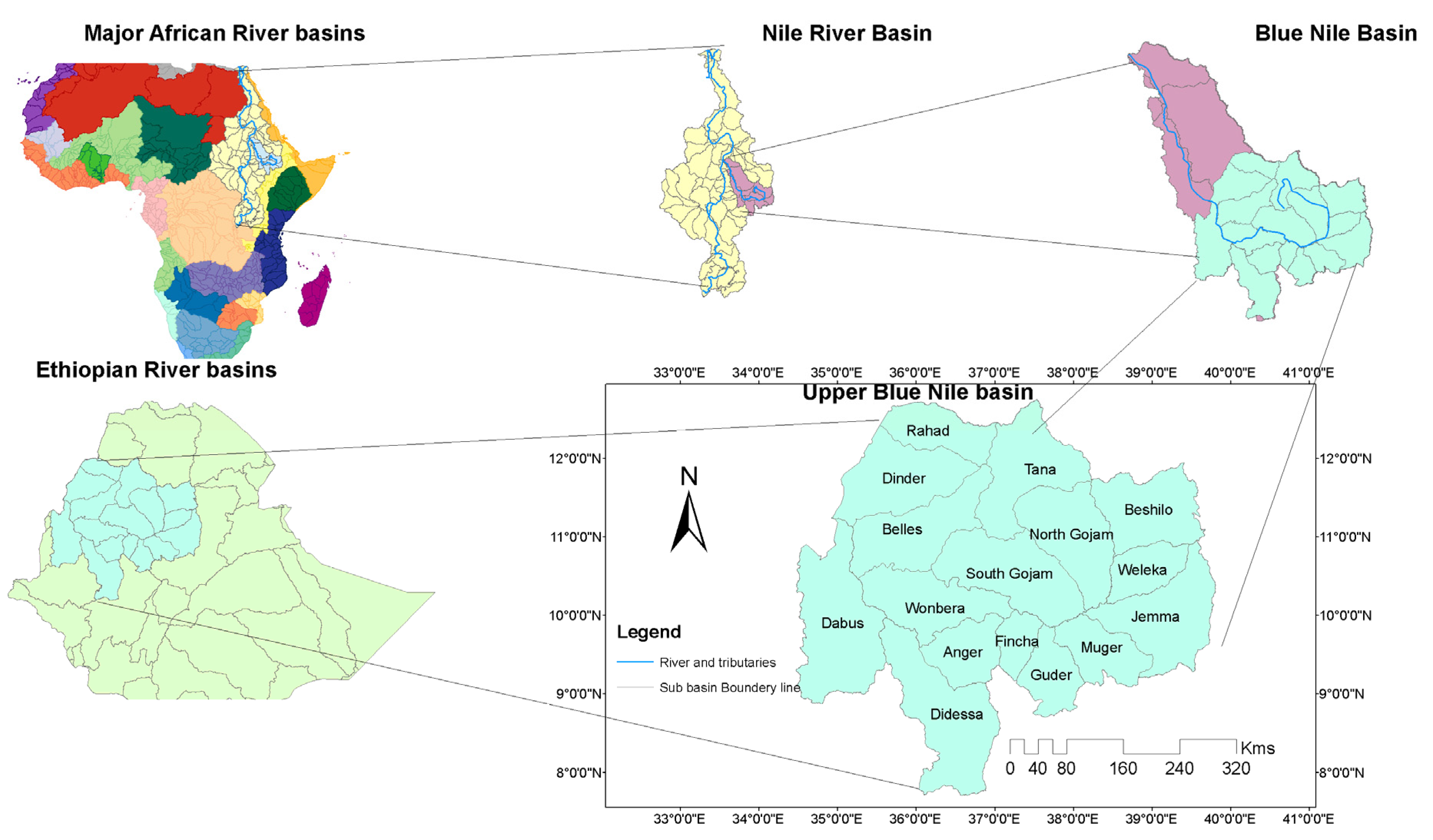
2.1. Study Area
2.2. Data Collection and Sources
2.2.1. GCM Outputs
2.2.2. Extreme Indices
2.2.3. Observed Data
3. Materials and Method
3.1. Representative Concentration Pathways Selection
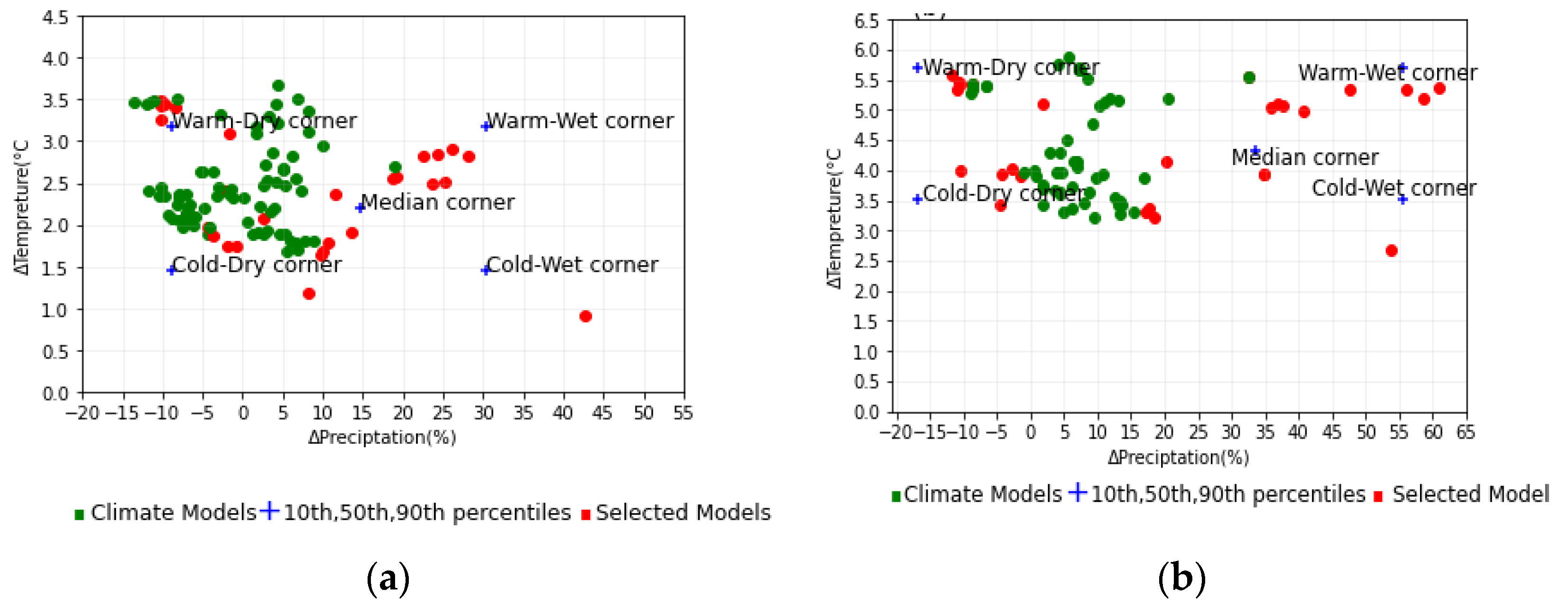
3.2. Climatic Means Changes
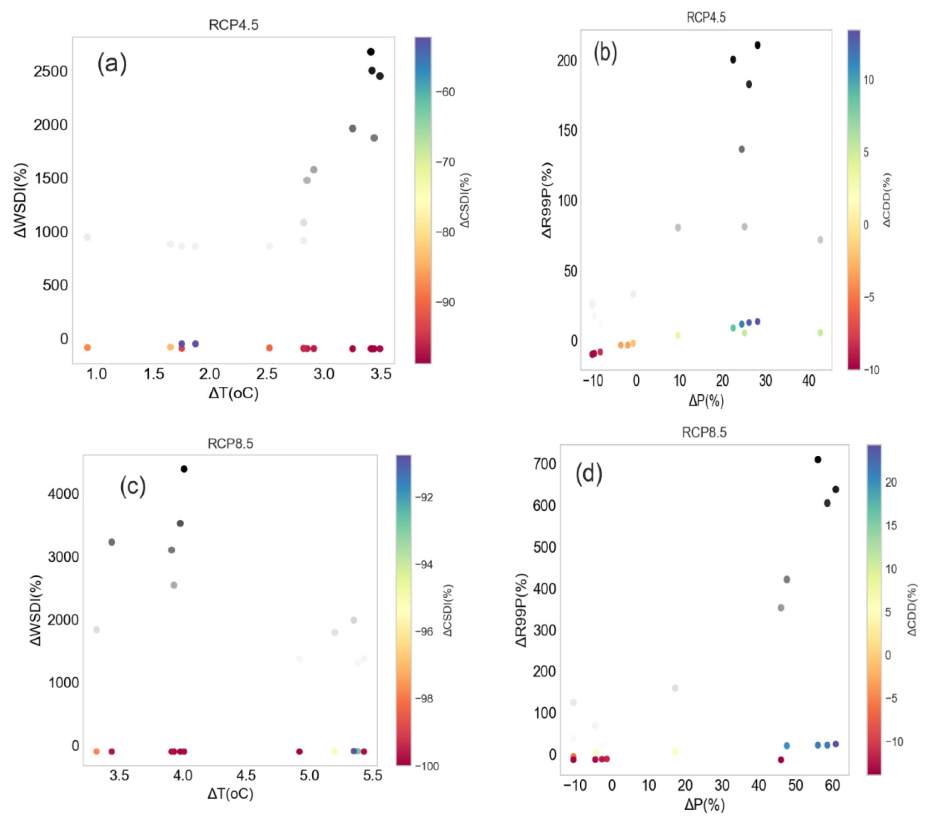
3.3. Refined Selection: Changes in Climatic Extremes
3.4. Past Performance
4. Results
4.1. Selection of Models
4.1.1. Changes in Climatic Means
4.1.2. Changes in Climatic Extremes
4.1.3. Past Performance
4.1.4. The Weighted Rank of the Overall Steps
4.2. Future Climate in the Upper Blue Nile Basin
5. Conclusions
Author Contributions
Funding
Institutional Review Board Statement
Informed Consent Statement
Data Availability Statement
Acknowledgments
Conflicts of Interest
References
- Taylor, K.E.; Stouffer, R.J.; Meehl, G.A. An overview of CMIP5 and the experiment design. Bull. Am. Meteorol. Soc. 2012, 93, 485–498. [Google Scholar] [CrossRef] [Green Version]
- Baede, A.; van der Linden, P.; Verbruggen, A. Annex to IPCC Fourth Assessment Report. IPCC Fourth Assess. Rep. 2007, 75–104. [Google Scholar]
- van Vuuren, D.P.; Edmonds, J.; Kainuma, M.; Riahi, K.; Thomson, A.; Hibbard, K.; Hurtt, G.C.; Kram, T.; Krey, V.; Lamarque, J.F.; et al. The representative concentration pathways: An overview. Clim. Chang. 2011, 109, 5–31. [Google Scholar] [CrossRef]
- Bjørnæs, C. A Guide to Representative Concentration Pathways History of Scenarios Year Name Used in 1990 SA90 First Assessment Report 1992 IS92 Second Assessment Report 2000 SRES—Special Report on Emissions and Scenarios Third and Four Assessment Report 2009 RCP. 2010. Available online: https://mpimet.mpg.de/fileadmin/communication/Im_Fokus/2013/IPCC_2013/uk_ipcc_A_guide_to_RCPs.pdf. (accessed on 22 February 2021).
- Jubb, A.I.; Canadell, P.; Dix, M. Representative Concentration Pathways (RCPs). Aust. Clim. Chang. Sci. Progr. 2013, 5–7. [Google Scholar]
- Lutz, A.F.; ter Maat, H.W.; Biemans, H.; Shrestha, A.B.; Wester, P.; Immerzeel, W.W. Selecting representative climate models for climate change impact studies: An advanced envelope-based selection approach. Int. J. Climatol. 2016, 36, 3988–4005. [Google Scholar] [CrossRef] [Green Version]
- Chen, J.; Brissette, F.P.; Leconte, R. Uncertainty of downscaling method in quantifying the impact of climate change on hydrology. J. Hydrol. 2011, 401, 190–202. [Google Scholar] [CrossRef]
- Chen, J.; Brissette, F.P.; Chaumont, D.; Braun, M. Performance and uncertainty evaluation of empirical downscaling methods in quantifying the climate change impacts on hydrology over two North American river basins. J. Hydrol. 2013, 479, 200–214. [Google Scholar] [CrossRef]
- Pryor, S.C.; Barthelmie, R.J.; Clausen, N.E.; Drews, M.; MacKellar, N.; Kjellström, E. Analyses of possible changes in intense and extreme wind speeds over northern Europe under climate change scenarios. Clim. Dyn. 2012, 38, 189–208. [Google Scholar] [CrossRef]
- Pour, S.H.; Shahid, S.; Chung, E.S.; Wang, X.J. Model output statistics downscaling using support vector machine for the projection of spatial and temporal changes in rainfall of Bangladesh. Atmos. Res. 2018, 213, 149–162. [Google Scholar] [CrossRef]
- Nikiema, P.M.; Sylla, M.B.; Ogunjobi, K.O.; Kebe, I.; Gibba, P.; Giorgi, F.; Omondi, C.K.; Huth, R.; Beck, C.; Philipp, A.; et al. Comparison of a very-fine-resolution GCM with RCM dynamical downscaling in simulating climate in China. J. Hydrol. 2016, 33, 559–570. [Google Scholar] [CrossRef] [Green Version]
- Khan, N.; Shahid, S.; Ahmed, K.; Ismail, T.; Nawaz, N.; Son, M. Performance assessment of general circulation model in simulating daily precipitation and temperature using multiple gridded datasets. Water 2018, 10, 1793. [Google Scholar] [CrossRef] [Green Version]
- McSweeney, C.F.; Jones, R.G.; Lee, R.W.; Rowell, D.P. Selecting CMIP5 GCMs for downscaling over multiple regions. Clim. Dyn. 2015, 44, 3237–3260. [Google Scholar] [CrossRef] [Green Version]
- Khan, A.J.; Koch, M. Selecting and downscaling a set of climate models for projecting climatic change for impact assessment in the Upper Indus Basin (UIB). Climate 2018, 6, 89. [Google Scholar] [CrossRef] [Green Version]
- Ahmed, K.; Shahid, S.; Sachindra, D.A.; Nawaz, N.; Chung, E.S. Fidelity assessment of general circulation model simulated precipitation and temperature over Pakistan using a feature selection method. J. Hydrol. 2019, 573, 281–298. [Google Scholar] [CrossRef]
- Betrie, G.D.; Mohamed, Y.A.; Van Griensven, A.; Srinivasan, R. Sediment management modelling in the Blue Nile Basin using SWAT model. Hydrol. Earth Syst. Sci. 2011, 15, 807–818. [Google Scholar] [CrossRef] [Green Version]
- Conway, D. The climate and hydrology of the Upper Blue Nile river. Geogr. J. 2000, 166, 49–62. [Google Scholar] [CrossRef] [Green Version]
- Mohamed, Y.A.; van den Hurk, B.J.J.M.; Savenije, H.H.G.; Bastiaanssen, W.G.M. Hydroclimatology of the Nile: Results from a regional climate model. Hydrol. Earth Syst. Sci. 2005, 9, 263–278. [Google Scholar] [CrossRef] [Green Version]
- Roth, V.; Lemann, T.; Zeleke, G.; Subhatu, A.T.; Nigussie, T.K.; Hurni, H. Effects of climate change on water resources in the upper Blue Nile Basin of Ethiopia. Heliyon 2018, 4, e00771. [Google Scholar] [CrossRef] [Green Version]
- Taye, M.T.; Willems, P.; Block, P. Implications of climate change on hydrological extremes in the Blue Nile basin: A review. J. Hydrol. Reg. Stud. 2015, 4, 280–293. [Google Scholar] [CrossRef] [Green Version]
- Mellander, P.E.; Gebrehiwot, S.G.; Gärdenäs, A.I.; Bewket, W.; Bishop, K. Summer Rains and Dry Seasons in the Upper Blue Nile Basin: The Predictability of Half a Century of Past and Future Spatiotemporal Patterns. PLoS ONE 2013, 8, e68461. [Google Scholar] [CrossRef] [Green Version]
- Zaitchik, B.F.; Simane, B.; Habib, S.; Anderson, M.C.; Ozdogan, M.; Foltz, J.D. Building climate resilience in the Blue Nile/Abay Highlands: A role for earth system sciences. Int. J. Environ. Res. Public Health 2012, 9, 435–461. [Google Scholar] [CrossRef] [PubMed] [Green Version]
- Sillmann, J.; Kharin, V.V.; Zhang, X.; Zwiers, F.W.; Bronaugh, D. Climate extremes indices in the CMIP5 multimodel ensemble: Part 1. Model evaluation in the present climate. J. Geophys. Res. Atmos. 2013, 118, 1716–1733. [Google Scholar] [CrossRef]
- Peterson, T.C.; Folland, C.; Gruza, G.; Hogg, W.; Mokssit, A.; Plummer, N. National Climatic Data Center, National Oceanic and Atmospheric Administration, Asheville, North Carolina, USA, and Chair, WMO Commission for Climatology Open Programme Area Group on the Monitoring and Analysis of Climate Variability and Change. Clim. Chang. Detect. 2001, 54, 143. [Google Scholar]
- Weedon, G.P.; Balsamo, G.; Bellouin, N.; Gomes, S.; Best, M.J.; Viterbo, P. The WFDEI meteorological forcing data set: WATCH Forcing data methodology applied to ERA-Interim reanalysis data. Water Resour. Res. 2014, 50, 7505–7514. [Google Scholar] [CrossRef] [Green Version]
- Weedon, G.P.; Gomes, S.; Viterbo, P.; Shuttleworth, W.J.; Blyth, E.; ÖSterle, H.; Adam, J.C.; Bellouin, N.; Boucher, O.; Best, M. Creation of the WATCH forcing data and its use to assess global and regional reference crop evaporation over land during the twentieth century. J. Hydrometeorol. 2011, 12, 823–848. [Google Scholar] [CrossRef] [Green Version]
- Dee, D.P.; Uppala, S.M.; Simmons, A.J.; Berrisford, P.; Poli, P.; Kobayashi, S.; Andrae, U.; Balmaseda, M.A.; Balsamo, G.; Bauer, P.; et al. The ERA-Interim reanalysis: Configuration and performance of the data assimilation system. Q. J. R. Meteorol. Soc. 2011, 137, 553–597. [Google Scholar] [CrossRef]
- Schneider, U.; Becker, A.; Finger, P.; Meyer-Christoffer, A.; Ziese, M.; Rudolf, B. GPCC’s new land surface precipitation climatology based on quality-controlled in situ data and its role in quantifying the global water cycle. Theor. Appl. Climatol. 2014, 115, 15–40. [Google Scholar] [CrossRef] [Green Version]
- Beaumont, L.J.; Hughes, L.; Pitman, A.J. Why is the choice of future climate scenarios for species distribution modelling important? Ecol. Lett. 2008, 11, 1135–1146. [Google Scholar] [CrossRef]
- Wayne, G.P. Representative Concentration Pathways. Available online: https://skepticalscience.com/docs/RCP_Guide.pdf. (accessed on 22 February 2021).
- Riahi, K.; Rao, S.; Krey, V.; Cho, C.; Chirkov, V.; Fischer, G.; Kindermann, G.; Nakicenovic, N.; Rafaj, P. RCP 8.5—A scenario of comparatively high greenhouse gas emissions. Clim. Chang. 2011, 109, 33–57. [Google Scholar] [CrossRef] [Green Version]
- Thomson, A.M.; Calvin, K.V.; Smith, S.J.; Kyle, G.P.; Volke, A.; Patel, P.; Delgado-Arias, S.; Bond-Lamberty, B.; Wise, M.A.; Clarke, L.E.; et al. RCP4.5: A pathway for stabilization of radiative forcing by 2100. Clim. Chang. 2011, 109, 77–94. [Google Scholar] [CrossRef] [Green Version]
- van Vuuren, D.P.; Stehfest, E.; den Elzen, M.G.J.; Kram, T.; van Vliet, J.; Deetman, S.; Isaac, M.; Goldewijk, K.K.; Hof, A.; Beltran, A.M.; et al. RCP2.6: Exploring the possibility to keep global mean temperature increase below 2 °C. Clim. Chang. 2011, 109, 95–116. [Google Scholar] [CrossRef]
- van Vuuren, D.P.; Stehfest, E.; den Elzen, M.G.J.; van Vliet, J.; Isaac, M. Exploring IMAGE model scenarios that keep greenhouse gas radiative forcing below 3 W/m2 in 2100. Energy Econ. 2010, 32, 1105–1120. [Google Scholar] [CrossRef]
- Wilby, R.L.; Dawson, C.W.; Murphy, C.; O’Connor, P.; Hawkins, E. The Statistical DownScaling Model -Decision Centric (SDSM-DC): Conceptual basis and applications. Clim. Res. 2014, 61, 251–268. [Google Scholar] [CrossRef] [Green Version]
- Pielke, R.A.; Wilby, R.L. Regional climate downscaling: What’s the point? Eos 2012, 93, 52–53. [Google Scholar] [CrossRef]
- Immerzeel, W.W.; Pellicciotti, F.; Bierkens, M.F.P. Rising river flows throughout the twenty-first century in two Himalayan glacierized watersheds. Nat. Geosci. 2013, 6, 742–745. [Google Scholar] [CrossRef]
- Sorg, A.; Huss, M.; Rohrer, M.; Stoffel, M. The days of plenty might soon be over in glacierized Central Asian catchments. Environ. Res. Lett. 2014, 9, 104018. [Google Scholar] [CrossRef]
- Murray, V.; Ebi, K.L. IPCC Special Report on Managing the Risks of Extreme Events and Disasters to Advance Climate Change Adaptation (SREX). J. Epidemiol. Community Health 2012, 66, 759–760. [Google Scholar] [CrossRef]
- Perkins, S.E.; Pitman, A.J.; Holbrook, N.J.; McAneney, J. Evaluation of the AR4 climate models’ simulated daily maximum temperature, minimum temperature, and precipitation over Australia using probability density functions. J. Clim. 2007, 20, 4356–4376. [Google Scholar] [CrossRef]
- Sáanchez, E.; Romera, R.; Gaertner, M.A.; Gallardo, C.; Castro, M. A weighting proposal for an ensemble of regional climate models over Europe driven by 1961-2000 ERA40 based on monthly precipitation probability density functions. Atmos. Sci. Lett. 2009, 10, 241–248. [Google Scholar] [CrossRef]
- Kjellström, E.; Boberg, F.; Castro, M.; Christensen, J.H.; Nikulin, G.; Sánchez, E. Daily and monthly temperature and precipitation statistics as performance indicators for regional climate models. Clim. Res. 2010, 44, 135–150. [Google Scholar] [CrossRef]
- Chen, J.; Brissette, F.P.; Lucas-Picher, P.; Caya, D. Impacts of weighting climate models for hydro-meteorological climate change studies. J. Hydrol. 2017, 549, 534–546. [Google Scholar] [CrossRef]
- Bhaskar, R.; Srinivas, D.; Ratna, S.B. Development of a high resolution daily gridded temperature data set (1969–2005) for the Indian region. Atmos. Sci. Lett. 2009, 10, 249–254. [Google Scholar] [CrossRef]
- Dufresne, J.L.; Foujols, M.A.; Denvil, S.; Caubel, A.; Marti, O.; Aumont, O.; Balkanski, Y.; Bekki, S.; Bellenger, H.; Benshila, R.; et al. Climate Change projections Using the IPSL-CM5 Earth System Model: From CMIP3 to CMIP5; Climate Dynamics: Paris, France, 2013; Volume 40, ISBN 0038201216. [Google Scholar]
- Ji, D.; Wang, L.; Feng, J.; Wu, Q.; Cheng, H.; Zhang, Q.; Yang, J.; Dong, W.; Dai, Y.; Gong, D.; et al. Description and basic evaluation of Beijing Normal University Earth System Model (BNU-ESM) version 1. Geosci. Model Dev. 2014, 7, 2039–2064. [Google Scholar] [CrossRef] [Green Version]
- Rotstayn, L.D.; Collier, M.A.; Dix, M.R.; Feng, Y.; Gordon, H.B.; O’Farrell, S.P.; Smith, I.N.; Syktus, J. Improved simulation of Australian climate and ENSO-related rainfall variability in a global climate model with an interactive aerosol treatment. Int. J. Climatol. 2010, 30, 1067–1088. [Google Scholar] [CrossRef]
- Volodin, E.M.; Dianskii, N.A.; Gusev, A.V. Simulating present-day climate with the INMCM4.0 coupled model of the atmospheric and oceanic general circulations. Izv. Atmos. Ocean Phys. 2010, 46, 414–431. [Google Scholar] [CrossRef]
- Wu, T.; Li, W.; Ji, J.; Xin, X.; Li, L.; Wang, Z.; Zhang, Y.; Li, J.; Zhang, F.; Wei, M.; et al. Global carbon budgets simulated by the Beijing Climate Center Climate System Model for the last century. J. Geophys. Res. Atmos. 2013, 118, 4326–4347. [Google Scholar] [CrossRef]
- Xin, X.G.; Wu, T.W.; Zhang, J. Introduction of CMIP5 experiments carried out with the climate system models of Beijing climate center. Adv. Clim. Chang. Res. 2013, 4, 41–49. [Google Scholar] [CrossRef]
- Rotstayn, L.D.; Jeffrey, S.J.; Collier, M.A.; Dravitzki, S.M.; Hirst, A.C.; Syktus, J.I.; Wong, K.K. Aerosol- and greenhouse gas-induced changes in summer rainfall and circulation in the Australasian region: A study using single-forcing climate simulations. Atmos. Chem. Phys. 2012, 12, 6377–6404. [Google Scholar] [CrossRef] [Green Version]
- Arora, V.K.; Scinocca, J.F.; Boer, G.J.; Christian, J.R.; Denman, K.L.; Flato, G.M.; Kharin, V.V.; Lee, W.G.; Merryfield, W.J. Carbon emission limits required to satisfy future representative concentration pathways of greenhouse gases. Geophys. Res. Lett. 2011, 38, 3–8. [Google Scholar] [CrossRef]
- Von Salzen, K.; Scinocca, J.F.; McFarlane, N.A.; Li, J.; Cole, J.N.S.; Plummer, D.; Verseghy, D.; Reader, M.C.; Ma, X.; Lazare, M.; et al. The Canadian fourth generation atmospheric global climate model (CanAM4). Part I: Representation of physical processes. Atmos. Ocean 2013, 51, 104–125. [Google Scholar] [CrossRef] [Green Version]


| Climate Variable | ETCCDI Index | Description of the ETCCDI Index |
|---|---|---|
| Precipitation | R99pTOT | Precipitation as a result of exceptionally wet days (>99th percentile) |
| CDD | Maximum length of a dry spell (P < 1 mm): consecutive dry days | |
| Air Temperature | WSDI | Warm spell duration index: the number of days in a period of at least six days where the daily maximum temperature (TX) is greater than the 90th percentile. |
| CSDI | Cold spell duration index: the number of days in a period of at least six days where the daily minimum temperature (TN) is less than in the tenth percentile. |
| Scenario | RCP4.5 | RCP8.5 | ||||
|---|---|---|---|---|---|---|
| RCP Projection | Model | ΔP (%) | ΔT (°C) | Model | ΔP (%) | ΔT (°C) |
| Warm-Dry | CSIRO-Mk3-6-0_r8i1p1 | −10.22 | 3.25 | CSIRO-Mk3-6-0_r4i1p1 | −11.7 | 5.58 |
| CSIRO-Mk3-6-0_r3i1p1 | −8.35 | 3.41 | CSIRO-Mk3-6-0_r1i1p1 | −10.7 | 5.47 | |
| CSIRO-Mk3-6-0_r6i1p1 | −9.75 | 3.44 | CSIRO-Mk3-6-0_r8i1p1 | −11.8 | 5.25 | |
| CSIRO-Mk3-6-0_r1i1p1 | −10.24 | 3.42 | CSIRO-Mk3-6-0_r2i1p1 | −10.5 | 5.43 | |
| CSIRO-Mk3-6-0_r2i1p1 | −10.08 | 3.49 | CSIRO-Mk3-6-0_r7i1p1 | −11 | 5.33 | |
| Cold-Dry | GFDL-ESM2G_r1i1p1 | −0.71 | 1.75 | GISS-E2-H_r1i1p1 | −10.5 | 3.98 |
| FIO-ESM_r3i1p1 | −4.37 | 1.9 | GISS-E2-R_r1i1p1 | −4.5 | 3.44 | |
| GISS-E2-R_r5i1p1 | −3.59 | 1.87 | GISS-E2-H_r1i1p2 | −4.23 | 3.93 | |
| FIO-ESM_r2i1p1 | −4.3 | 1.97 | GFDL-ESM2G_r1i1p1 | −1.4 | 3.91 | |
| inmcm4_r1i1p1 | −2.00 | 1.75 | FIO-ESM_r2i1p1 | −2.71 | 4.01 | |
| Cold-Wet | CanESM2_r5i1p1 | 23.68 | 2.48 | BNU-ESM_r1i1p1 | 53.69 | 2.69 |
| BNU-ESM_r1i1p1 | 42.66 | 0.92 | FGOALS_g2_r1i1p1 | 20.19 | 2.41 | |
| FGOALS_g2_ r1i1p1 | 8.24 | 1.19 | CESM1-BGC_r1i1p1 | 18.48 | 3.21 | |
| CCSM4_r4i1p1 | 9.99 | 1.69 | CCSM4_r6i1p1 | 17.73 | 3.36 | |
| CCSM4_r2i1p1 | 9.68 | 1.65 | CCSM4_r2i1p1 | 17.15 | 3.32 | |
| Warm-Wet | IPSL-CM5A-LR_r3i1p1 | 26.17 | 2.91 | IPSL-CM5A-LR_r2i1p1 | 56.03 | 5.35 |
| IPSL-CM5A-LR_r1i1p1 | 28.12 | 2.82 | IPSL-CM5A-LR_r1i1p1 | 60.83 | 5.38 | |
| IPSL-CM5A-LR_r4i1p1 | 24.42 | 2.85 | IPSL-CM5A-LR_r3i1p1 | 47.55 | 5.35 | |
| IPSL-CM5A-LR_r2i1p1 | 22.42 | 2.82 | IPSL-CM5A-LR_r4i1p1 | 58.57 | 5.2 | |
| CanESM2_r4i1p1 | 25.12 | 2.52 | CanESM2_r5i1p1 | 45.94 | 4.92 | |
| IPSL-CM5A-LR_r3i1p1 | 26.17 | 2.91 | IPSL-CM5A-LR_r2i1p1 | 56.03 | 5.35 | |
| Mean (50th percentile) | CESM1-CAM5_r2i1p1 | 11.54 | 2.36 | CanESM2_r1i1p1 | 37.67 | 5.06 |
| bcc-csm1-1-m_r1i1p1 | 10.73 | 1.78 | CanESM2_r2i1p1 | 36.95 | 5.09 | |
| CanESM2_r3i1p1 | 19.16 | 2.58 | CanESM2_r3i1p1 | 35.94 | 5.04 | |
| CanESM2_r1i1p1 | 18.72 | 2.56 | CanESM2_r4i1p1 | 40.82 | 4.97 | |
| IPSL-CM5B-LR_r1i1p1 | 13.59 | 1.92 | IPSL-CM5B-LR_r1i1p1 | 34.77 | 3.94 |
| RCP Projection | Model | ΔR99P Tot (%) | ΔCDD (%) | ΔWSDI (%) | ΔCSDI (%) |
|---|---|---|---|---|---|
| Warm-Dry | CSIRO-Mk3-6-0_r8i1p1 | 26.35 | −10.02 | 1959.46 | −98.07 |
| CSIRO-Mk3-6-0_r3i1p1 | 12.57 | −8.31 | 2677.96 | −97.48 | |
| CSIRO-Mk3-6-0_r6i1p1 | 17.59 | −9.34 | 1871.25 | −98.22 | |
| CSIRO-Mk3-6-0_r1i1p1 | 24.91 | −9.77 | 2501.96 | −98.78 | |
| CSIRO-Mk3-6-0_r2i1p1 | 25.92 | −9.74 | 2451.11 | −98.05 | |
| Cold-Dry | GFDL-ESM2G_r1i1p1 | 32.9 | −2.1 | 634.53 | −93.63 |
| FIO-ESM_r3i1p1 | __ | __ | __ | __ | |
| GISS-E2-R_r5i1p1 | __ | __ | __ | __ | |
| FIO-ESM_r2i1p1 | __ | __ | __ | __ | |
| inmcm4_r1i1p1 | 5.41 | −3.34 | 858.61 | −52.22 | |
| Wet-Cold | BNU-ESM_r1i1p1 | __ | __ | __ | __ |
| bcc-csm1-1-m_r1i1p1 | 71.71 | 5.36 | 944.7 | −87.52 | |
| FGOALS_g2_ r1i1p1 | __ | __ | __ | __ | |
| CCSM4_r4i1p1 | __ | __ | __ | __ | |
| CCSM4_r2i1p1 | 80.39 | 3.46 | 879.57 | −83.52 | |
| Wet-Warm | IPSL-CM5A-LR_r3i1p1 | 182.56 | 12.66 | 1575.59 | −96.59 |
| IPSL-CM5A-LR_r1i1p1 | 210.48 | 13.43 | 1081.35 | −94.09 | |
| IPSL-CM5A-LR_r4i1p1 | 136.30 | 11.511 | 1476.11 | −96.55 | |
| IPSL-CM5A-LR_r2i1p1 | 200.19 | 8.766 | 914.82 | −95.67 | |
| CanESM2_r4i1p1 | 80.96 | 5.24 | 859.92 | −90.38 |
| RCP Projection | Model | ΔR99P Tot (%) | ΔCDD (%) | ΔWSDI (%) | ΔCSDI (%) |
|---|---|---|---|---|---|
| Warm-Dry | GISS-E2-H_r1i1p1 | ___ | ___ | ___ | ___ |
| GISS-E2-R_r1i1p1 | ___ | ___ | ___ | ___ | |
| GISS-E2-H_r1i1p2 | ___ | ___ | ___ | ___ | |
| GFDL-ESM2G_r1i1p1 | 124.26 | −5.99 | 1376.13 | −99.79 | |
| FIO-ESM_r2i1p1 | ___ | ___ | ___ | ___ | |
| Cold-Dry | CSIRO-Mk3-6-0_r4i1p1 | 37.83 | −13.58 | 3525.97 | −99.98 |
| CSIRO-Mk3-6-0_r1i1p1 | 68.59 | −13.19 | 3227.31 | −99.68 | |
| CSIRO-Mk3-6-0_r8i1p1 | 15.44 | 4.99 | 2546.26 | −100 | |
| CSIRO-Mk3-6-0_r2i1p1 | 3.05 | −11.49 | 3102.2 | −99.78 | |
| CSIRO-Mk3-6-0_r7i1p1 | 19.83 | −12.21 | 4388.02 | −99.85 | |
| Wet-Cold | BNU-ESM_r1i1p1 | ___ | ___ | ___ | ___ |
| FGOALS_g2_r1i1p1 | ___ | ___ | ___ | ___ | |
| CESM1-BGC_r1i1p1 | ___ | ___ | ___ | ___ | |
| CCSM4_r6i1p1 | ___ | ___ | ___ | ___ | |
| CCSM4_r2i1p1 | 158.93 | 5.49 | 1835.49 | −97.79 | |
| Wet-Warm | IPSL-CM5A-LR_r2i1p1 | 709.7 | 21.26 | 1094.01 | −94.79 |
| IPSL-CM5A-LR_r1i1p1 | 638 | 24.34 | 1305.77 | −92.69 | |
| IPSL-CM5A-LR_r3i1p1 | 420.94 | 19.96 | 1988.23 | −90.75 | |
| IPSL-CM5A-LR_r4i1p1 | 604.9 | 21.26 | 1791.89 | −95.09 | |
| CanESM2_r4i1p1 | 80.96 | 5.24 | 859.92 | −90.38 |
| Scenario | RCP4.5 | RCP8.5 | ||||
|---|---|---|---|---|---|---|
| RCP Projection | Model | Tscore | P Score | Model | Tscore | P Score |
| Warm-Dry | CSIRO-Mk3-6-0_r8i1p1 | 0.63 | 0.23 | CSIRO-Mk3-6-0_r4i1p1 | 0.55 | 0.36 |
| CSIRO-Mk3-6-0_r3i1p1 | 0.62 | 0.26 | CSIRO-Mk3-6-0_r1i1p1 | 0.52 | 0.39 | |
| CSIRO-Mk3-6-0_r6i1p1 | 0.55 | 0.25 | CSIRO-Mk3-6-0_r8i1p1 | 0.55 | 0.41 | |
| CSIRO-Mk3-6-0_r1i1p1 | 0.59 | 0.38 | CSIRO-Mk3-6-0_r2i1p1 | 0.55 | 0.16 | |
| CSIRO-Mk3-6-0_r2i1p1 | 0.65 | 0.24 | CSIRO-Mk3-6-0_r7i1p1 | 0.51 | 0.34 | |
| Cold-Dry | GFDL-ESM2G_r1i1p1 | 0.55 | 0.41 | GISS-E2-H_r1i1p1 | 0.66 | 0.25 |
| FIO-ESM_r3i1p1 | 0.53 | 0.43 | GISS-E2-R_r1i1p1 | 0.63 | 0.22 | |
| GISS-E2-R_r5i1p1 | 0.54 | 0.52 | GISS-E2-H_r1i1p2 | 0.68 | 0.03 | |
| FIO-ESM_r2i1p1 | 0.49 | 0.46 | GFDL-ESM2G_r1i1p1 | 0.66 | 0.22 | |
| inmcm4_r1i1p1 | 0.52 | 0.44 | FIO-ESM_r2i1p1 | 0.58 | 0.43 | |
| Cold-Warm | CanESM2_r5i1p1 | 0.58 | 0.40 | BNU-ESM_r1i1p1 | 0.64 | 0.36 |
| BNU-ESM_r1i1p1 | 0.64 | 0.35 | FGOALS_g2_r1i1p1 | 0.59 | 0.46 | |
| FGOALS_g2_r1i1p1 | 0.59 | 0.37 | CESM1-BGC_r1i1p1 | 0.6 | 0.21 | |
| CCSM4_r4i1p1 | 0.56 | 0.51 | CCSM4_r6i1p1 | 0.58 | 0.27 | |
| CCSM4_r2i1p1 | 0.60 | 0.51 | CCSM4_r2i1p1 | 0.60 | 0.45 | |
| Warm-Wet | IPSL-CM5A-LR_r3i1p1 | 0.60 | 0.35 | IPSL-CM5A-LR_r2i1p1 | 0.57 | 0.43 |
| IPSL-CM5A-LR_r1i1p1 | 0.64 | 0.35 | IPSL-CM5A-LR_r1i1p1 | 0.64 | 0.38 | |
| IPSL-CM5A-LR_r4i1p1 | 0.60 | 0.39 | IPSL-CM5A-LR_r3i1p1 | 0.46 | 0.14 | |
| IPSL-CM5A-LR_r2i1p1 | 0.57 | 0.39 | IPSL-CM5A-LR_r4i1p1 | 0.60 | 0.14 | |
| CanESM2_r4i1p1 | 0.57 | 0.32 | CanESM2_r5i1p1 | 0.58 | 0.40 | |
| CESM1-CAM5_r2i1p1 | 0.59 | 0.62 | CanESM2_r1i1p1 | 0.57 | 0.25 | |
| bcc-csm1-1-m_r1i1p1 | 0.62 | 0.44 | CanESM2_r2i1p1 | 0.49 | 0.44 | |
| Mean | CanESM2_r3i1p1 | 0.56 | 0.32 | CanESM2_r3i1p1 | 0.56 | 0.39 |
| CanESM2_r1i1p1 | 0.57 | 0.25 | CanESM2_r4i1p1 | 0.57 | 0.43 | |
| IPSL-CM5B-LR_r1i1p1 | 0.58 | 0.30 | IPSL-CM5B-LR_r1i1p1 | 0.58 | 0.27 |
| GCM Runs | Tana | North Gojam | Beshilo | Weleka | Jemma | South Gojam | Muger | Guder | Fincha | Didessa | Anger | Wonbera | Dabus | Belles | Dinder | Rahad | Guder |
|---|---|---|---|---|---|---|---|---|---|---|---|---|---|---|---|---|---|
| IPSL-CM5A-LR_r3i1p1 | 0.39 | 0.51 | 0.60 | 0.61 | 0.66 | 0.63 | 0.70 | 0.68 | 0.52 | 0.68 | 0.50 | 0.57 | 0.62 | 0.62 | 0.68 | ||
| BNU-ESM_r1i1p1 | 0.22 | 0.34 | 0.18 | 0.36 | 0.33 | 0.51 | 0.31 | 0.51 | 0.35 | 0.47 | 0.30 | 0.39 | 0.54 | 0.54 | 0.23 | ||
| CSIRO-Mk3-6-0_r3i1p1 | 0.38 | 0.40 | 0.29 | 0.36 | 0.36 | 0.47 | 0.42 | 0.35 | 0.42 | 0.50 | 0.35 | 0.70 | 0.11 | 0.11 | 0.76 | ||
| inmcm4_r1i1p1 | 0.20 | 0.18 | 0.21 | 0.41 | 0.35 | 0.29 | 0.32 | 0.36 | 0.23 | 0.43 | 0.22 | 0.26 | 0.63 | 0.63 | 0.25 | ||
| bcc-csm1-1-m-r1i1p1 | 0.29 | 0.22 | 0.18 | 0.23 | 0.31 | 0.40 | 0.38 | 0.44 | 0.37 | 0.49 | 0.32 | 0.41 | 0.28 | 0.28 | 0.39 | ||
| IPSL-CM5A-LR_r2i1p1 | 0.13 | 0.22 | 0.29 | 0.35 | 0.36 | 0.31 | 0.37 | 0.40 | 0.23 | 0.37 | 0.21 | 0.26 | 0.31 | 0.31 | 0.21 | ||
| CSIRO-Mk3-6-0_r4i1p1 | 0.33 | 0.46 | 0.18 | 0.35 | 0.34 | 0.46 | 0.42 | 0.31 | 0.49 | 0.45 | 0.40 | 0.66 | 0.13 | 0.13 | 0.58 | ||
| GFDL-ESM2G_r1i1p1 | 0.46 | 0.30 | 0.42 | 0.64 | 0.46 | 0.59 | 0.43 | 0.54 | 0.35 | 0.47 | 0.30 | 0.42 | 0.51 | 0.51 | 0.52 | ||
| CanESM2-r3i1p1 | 0.41 | 0.58 | 0.29 | 0.27 | 0.26 | 0.28 | 0.25 | 0.16 | 0.55 | 0.18 | 0.60 | 0.45 | 0.17 | 0.17 | 0.26 |
| GCM Runs | Tana | North Gojam | Beshilo | Weleka | Jemma | South Gojam | Muger | Guder | Fincha | Didessa | Anger | Wonbera | Dabus | Belles | Dinder | Rahad | Guder |
|---|---|---|---|---|---|---|---|---|---|---|---|---|---|---|---|---|---|
| IPSL-CM5A-LR_r3i1p1 | 0.46 | 0.57 | 0.63 | 0.63 | 0.58 | 0.58 | 0.56 | 0.69 | 0.60 | 0.66 | 0.61 | 0.65 | 0.67 | 0.60 | 0.59 | ||
| BNU-ESM_r1i1p1 | 0.35 | 0.43 | 0.60 | 0.56 | 0.55 | 0.63 | 0.56 | 0.66 | 0.66 | 0.65 | 0.65 | 0.63 | 0.72 | 0.66 | 0.69 | ||
| CSIRO-Mk3-6-0_r3i1p1 | 0.47 | 0.53 | 0.53 | 0.56 | 0.53 | 0.53 | 0.57 | 0.71 | 0.57 | 0.66 | 0.58 | 0.66 | 0.67 | 0.62 | 0.68 | ||
| inmcm4_r1i1p1 | 0.56 | 0.51 | 0.56 | 0.47 | 0.47 | 0.44 | 0.47 | 0.46 | 0.45 | 0.45 | 0.47 | 0.47 | 0.53 | 0.54 | 0.56 | ||
| bcc-csm1-1-m-r1i1p1 | 0.56 | 0.70 | 0.60 | 0.61 | 0.61 | 0.62 | 0.69 | 0.68 | 0.66 | 0.71 | 0.68 | 0.66 | 0.63 | 0.61 | 0.57 | ||
| IPSL-CM5A-LR_r2i1p1 | 0.46 | 0.53 | 0.58 | 0.59 | 0.60 | 0.56 | 0.55 | 0.66 | 0.57 | 0.68 | 0.61 | 0.61 | 0.66 | 0.58 | 0.61 | ||
| CSIRO-Mk3-6-0_r4i1p1 | 0.45 | 0.48 | 0.52 | 0.54 | 0.57 | 0.51 | 0.49 | 0.72 | 0.49 | 0.69 | 0.52 | 0.69 | 0.68 | 0.65 | 0.68 | ||
| GFDL-ESM2G_r1i1p1 | 0.58 | 0.59 | 0.62 | 0.61 | 0.58 | 0.65 | 0.61 | 0.64 | 0.64 | 0.64 | 0.63 | 0.68 | 0.69 | 0.70 | 0.65 | ||
| CanESM2-r3i1p1 | 0.53 | 0.62 | 0.51 | 0.54 | 0.52 | 0.61 | 0.50 | 0.63 | 0.64 | 0.62 | 0.61 | 0.60 | 0.60 | 0.64 | 0.64 |
| a | b | c | d | e | f | g | h | ||||
|---|---|---|---|---|---|---|---|---|---|---|---|
| Projection | Climate Model | Weighted Rank ∆R99pTOT (%) | Weighted Rank ∆CDD (%) | Weighted Rank ∆WSDI (%) | Weighted Rank ∆CSDI (%) | Weighted Rank ∆T (°C) | Weighted Rank ∆P (%) | Skill Score for Temperature (SkTmp) | Skill Score for Precipitation (SkPerc) | Final Skill Score (a ∗ b ∗ c ∗ d ∗ e ∗ f ∗ g ∗ h ∗ 10) | Final Rank |
| Wet-Warm | IPSL-CM5A-LR_r3i1p1 | 0.87 | --- | 1 | --- | 0.92 | 0.87 | 0.6 | 0.35 | 1.46 | 1 |
| IPSL-CM5A-LR_r1i1p1 | 1 | --- | 0.69 | --- | 0.89 | 0.93 | 0.64 | 0.35 | 1.27 | 2 | |
| IPSL-CM5A-LR_r4i1p1 | 0.65 | --- | 0.94 | --- | 0.9 | 0.81 | 0.6 | 0.39 | 1.02 | 3 | |
| IPSL-CM5A-LR_r2i1p1 | 0.95 | --- | 0.58 | --- | 0.89 | 0.74 | 0.57 | 0.39 | 0.82 | 4 | |
| CanESM2_r4i1p1 | 0.77 | -- | 0.55 | --- | 0.79 | 0.83 | 0.57 | 0.32 | 0.5 | 5 | |
| Wet-Cold | CanESM2_r5i1p1 | 0.7 | --- | --- | 0.96 | 0.3 | 0.78 | 0.58 | 0.4 | 0.36 | 4 |
| BNU-ESM_r1i1p1 | --- | --- | --- | --- | 0.63 | 0.59 | 0.64 | 0.35 | 0.84 | 1 | |
| FGOALS_g2_ r1i1p1 | --- | --- | --- | --- | 0.82 | 0.27 | 0.59 | 0.37 | 0.48 | 3 | |
| CCSM4_r4i1p1 | --- | --- | --- | --- | 0.84 | 0.33 | 0.56 | 0.51 | 0.8 | 2 | |
| CCSM4_r2i1p1 | 1 | 0.35 | 0.33 | 0.85 | 0.87 | 0.32 | 0.6 | 0.51 | 0.08 | 5 | |
| Dry-Warm | CSIRO-Mk3-6-0_r8i1p1 | --- | 1 | 0.73 | --- | 0.97 | 0.86 | 0.55 | 0.41 | 1.4 | 5 |
| CSIRO-Mk3-6-0_r3i1p1 | --- | 0.83 | 1 | --- | 0.92 | 0.93 | 0.53 | 0.43 | 1.614 | 1 | |
| CSIRO-Mk3-6-0_r6i1p1 | --- | 0.93 | 0.7 | --- | 0.91 | 0.91 | 0.54 | 0.52 | 1.53 | 4 | |
| CSIRO-Mk3-6-0_r1i1p1 | --- | 0.98 | 0.93 | --- | 0.92 | 0.86 | 0.49 | 0.46 | 1.613 | 2 | |
| CSIRO-Mk3-6-0_r2i1p1 | --- | 0.97 | 0.92 | --- | 0.9 | 0.87 | 0.52 | 0.44 | 1.59 | 3 | |
| Dry-Cold | GISS-E2-R_r1i1p1 | --- | 0.06 | --- | 0.95 | 0.64 | 0.83 | 0.63 | 0.23 | 0.04 | 5 |
| GISS-E2-R_r4i1p1 | --- | --- | --- | --- | 0.61 | 0.74 | 0.62 | 0.26 | 0.71 | 2 | |
| GISS-E2-R_r3i1p1 | --- | --- | --- | --- | 0.63 | 0.7 | 0.55 | 0.25 | 0.61 | 3 | |
| FIO-ESM_r3i1p1 | --- | --- | --- | --- | 0.7 | 0.49 | 0.59 | 0.38 | 0.77 | 1 | |
| inmcm4_r1i1p1 | --- | 1 | --- | 0.558 | 0.71 | 0.4 | 0.65 | 0.24 | 0.25 | 4 | |
| Mean | CESM1-CAM5_r2i1p1 | --- | --- | --- | --- | 0.93 | 0.79 | 0.59 | 0.62 | 2.69 | 1 |
| bcc-csm1-1-m_r1i1p1 | --- | --- | --- | --- | 0.81 | 0.73 | 0.62 | 0.44 | 1.62 | 2 | |
| CanESM2_r3i1p1 | --- | --- | --- | --- | 0.83 | 0.69 | 0.56 | 0.32 | 1.02 | 4 | |
| CanESM2_r1i1p1 | --- | --- | --- | --- | 0.84 | 0.72 | 0.57 | 0.25 | 0.87 | 5 | |
| IPSL-CM5B-LR_r1i1p1 | --- | --- | --- | --- | 0.87 | 0.93 | 0.58 | 0.3 | 1.41 | 3 |
| a | b | c | d | e | f | g | h | ||||
|---|---|---|---|---|---|---|---|---|---|---|---|
| Projection | Climate Model | Weighted Rank ∆R99pTOT (%) | Weighted Rank ∆CDD (%) | Weighted Rank ∆WSDI (%) | Weighted Rank ∆CSDI (%) | Weighted Rank ∆T (°C) | Weighted Rank ∆P (%) | Skill Score for Temperature (SkTmp) | Skill Score for Precipitation (SkPerc) | Final Skill Score (a ∗ b ∗ c ∗ d ∗ e ∗ f ∗ g ∗ h ∗ 10) | Final Rank |
| Warm-Dry | CSIRO-Mk3-6-0_r4i1p1 | --- | 1 | 0.8 | --- | 0.98 | 0.7 | 0.55 | 0.36 | 1.08 | 1 |
| CSIRO-Mk3-6-0_r1i1p1 | --- | 0.97 | 0.74 | --- | 0.96 | 0.64 | 0.52 | 0.39 | 0.89 | 3 | |
| CSIRO-Mk3-6-0_r8i1p1 | --- | 0.37 | 0.58 | --- | 0.92 | 0.7 | 0.55 | 0.41 | 0.31 | 4 | |
| CSIRO-Mk3-6-0_r2i1p1 | --- | 0.85 | 0.71 | --- | 0.95 | 0.63 | 0.55 | 0.16 | 0.3 | 5 | |
| CSIRO-Mk3-6-0_r7i1p1 | --- | 0.9 | 1 | --- | 0.94 | 0.66 | 0.51 | 0.34 | 0.96 | 2 | |
| Cold-Dry | GISS-E2-H_r1i1p1 | --- | --- | --- | --- | 0.87 | 0.37 | 0.66 | 0.25 | 0.52 | 4 |
| GISS-E2-R_r1i1p1 | --- | --- | --- | --- | 0.98 | 0.73 | 0.63 | 0.22 | 1.01 | 3 | |
| GISS-E2-H_r1i1p2 | --- | --- | --- | --- | 0.88 | 0.75 | 0.68 | 0.03 | 0.15 | 5 | |
| GFDL-ESM2G_r1i1p1 | 1 | 1 | --- | 1 | 0.88 | 0.92 | 0.66 | 0.22 | 1.17 | 2 | |
| FIO-ESM_r2i1p1 | --- | --- | --- | --- | 0.86 | 0.84 | 0.58 | 0.43 | 1.79 | 1 | |
| Cold-Warm | BNU-ESM_r1i1p1 | --- | --- | --- | --- | 0.77 | 0.97 | 0.64 | 0.36 | 1.69 | 1 |
| FGOALS_g2_r1i1p1 | --- | --- | --- | --- | 0.69 | 0.36 | 0.59 | 0.46 | 0.67 | 3 | |
| CESM1-BGC_r1i1p1 | --- | --- | --- | --- | 0.91 | 0.33 | 0.6 | 0.21 | 0.38 | 5 | |
| CCSM4_r6i1p1 | --- | --- | --- | --- | 0.96 | 0.32 | 0.58 | 0.27 | 0.48 | 4 | |
| CCSM4_r2i1p1 | 1 | --- | --- | 0.98 | 0.95 | 0.31 | 0.6 | 0.45 | 0.77 | 2 | |
| Warm-Wet | IPSL-CM5A-LR_r2i1p1 | 1 | --- | 0.55 | --- | 0.94 | 0.99 | 0.57 | 0.43 | 1.27 | 1 |
| IPSL-CM5A-LR_r1i1p1 | 0.9 | --- | 0.66 | --- | 0.94 | 0.91 | 0.64 | 0.38 | 1.22 | 2 | |
| IPSL-CM5A-LR_r3i1p1 | 0.59 | --- | 1 | --- | 0.94 | 0.86 | 0.46 | 0.14 | 0.31 | 5 | |
| IPSL-CM5A-LR_r4i1p1 | 0.85 | --- | 0.9 | --- | 0.91 | 0.95 | 0.6 | 0.14 | 0.567 | 4 | |
| CanESM2_r5i1p1 | 1 | --- | 0.55 | --- | 0.94 | 0.99 | 0.57 | 0.43 | 1.27 | 1 | |
| Mean | CanESM2_r1i1p1 | --- | --- | --- | --- | 0.83 | 0.88 | 0.573 | 0.25 | 1.05 | 5 |
| CanESM2_r2i1p1 | --- | --- | --- | --- | 0.82 | 0.9 | 0.49 | 0.44 | 1.61 | 3 | |
| CanESM2_r3i1p1 | --- | --- | --- | --- | 0.83 | 0.93 | 0.563 | 0.39 | 1.72 | 1 | |
| CanESM2_r4i1p1 | --- | --- | --- | --- | 0.85 | 0.79 | 0.567 | 0.43 | 1.63 | 2 | |
| IPSL-CM5B-LR_r1i1p1 | --- | --- | --- | --- | 0.91 | 0.97 | 0.577 | 0.27 | 1.37 | 4 |
| Scenario | Projection | Model | ΔT (°C) | ΔP (%) | ΔWSDI (%) | ΔCSDI (%) | ΔR99P (%) | ΔCDD (%) |
|---|---|---|---|---|---|---|---|---|
| RCP4.5 | Wet-Warm | IPSL-CM5A-LR_r3i1p1 | 2.91 | 26.17 | 1575.59 | −96.59 | 182.56 | 12.66 |
| Wet-Cold | BNU-ESM_r1i1p1 | 0.92 | 42.66 | --- | --- | --- | --- | |
| Dry-Warm | CSIRO-Mk3-6-0_r3i1p1 | 3.41 | −8.35 | 2677.96 | −97.48 | 12.57 | −8.31 | |
| Dry-Cold | inmcm4_r1i1p1 | 1.75 | −2.00 | 858.61 | −52.22 | 5.41 | −3.34 | |
| RCP8.5 | Wet-Warm | IPSL-CM5A-LR_r2i1p1 | 5.35 | 56.03 | 1094.01 | −94.79 | 709.70 | 21.26 |
| Wet-Cold | BNU-ESM_r1i1p1 | 2.69 | 53.69 | --- | --- | --- | --- | |
| Dry-Warm | CSIRO-Mk3-6-0_r4i1p1 | 5.58 | −11.70 | 3525.97 | −99.98 | 37.83 | −13.58 | |
| Dry-Cold | GFDL-ESM2G_r1i1p1 | 3.91 | −1.40 | 1376.13 | −99.79 | 124.26 | −5.99 |
| Scenario | Model Name | Institute | Ensembles | References |
|---|---|---|---|---|
| IPSL-CM5A-LR | Institut Pierre Simon Laplace, Paris, France | r3i1p | [45] | |
| BNU-ESM | GCESS, BNU, Beijing, China | r1i1p1 | [46] | |
| RCP4.5 | CSIRO-Mk3-6-0 | CSIRO Marine and Atmospheric Research | r3i1p1 | [47] |
| inmcm4_ | Institute for Numerical Mathematics, Moscow, | r1i1p1 | [48] | |
| bcc-csm1-1-m | Beijing Climate Center | r1i1p1 | [49,50] | |
| IPSL-CM5A-LR | Institut Pierre Simon Laplace, Paris, France | r2i1p1 | [45] | |
| RCP8.5 | BNU-ESM_ | GCESS, BNU, Beijing, China | r1i1p1 | [46] |
| CSIRO-Mk3-6-0 | CSIRO Marine and Atmospheric Research | r4i1p1 | [47] | |
| GFDL-ESM2G | NOAA Geophysical Fluid Dynamics Laboratory | r1i1p1 | [51] | |
| CanESM2 | Canadian Center for Climate Modeling and Analysis | r3i1p1 | [52,53] |
Publisher’s Note: MDPI stays neutral with regard to jurisdictional claims in published maps and institutional affiliations. |
© 2022 by the authors. Licensee MDPI, Basel, Switzerland. This article is an open access article distributed under the terms and conditions of the Creative Commons Attribution (CC BY) license (https://creativecommons.org/licenses/by/4.0/).
Share and Cite
Tenfie, H.W.; Saathoff, F.; Hailu, D.; Gebissa, A. Selection of Representative General Circulation Models for Climate Change Study Using Advanced Envelope-Based and Past Performance Approach on Transboundary River Basin, a Case of Upper Blue Nile Basin, Ethiopia. Sustainability 2022, 14, 2140. https://doi.org/10.3390/su14042140
Tenfie HW, Saathoff F, Hailu D, Gebissa A. Selection of Representative General Circulation Models for Climate Change Study Using Advanced Envelope-Based and Past Performance Approach on Transboundary River Basin, a Case of Upper Blue Nile Basin, Ethiopia. Sustainability. 2022; 14(4):2140. https://doi.org/10.3390/su14042140
Chicago/Turabian StyleTenfie, Hailu Wondmageghu, Fokke Saathoff, Dereje Hailu, and Alemayehu Gebissa. 2022. "Selection of Representative General Circulation Models for Climate Change Study Using Advanced Envelope-Based and Past Performance Approach on Transboundary River Basin, a Case of Upper Blue Nile Basin, Ethiopia" Sustainability 14, no. 4: 2140. https://doi.org/10.3390/su14042140