Day-Ahead Wind Power Forecasting Based on Wind Load Data Using Hybrid Optimization Algorithm

Abstract

Accurate wind power forecasting is essential to reduce the negative impact of wind power on the operation of the grid and the operation cost of the power system. Day-ahead wind power forecasting plays an important role in the day-ahead electricity spot trading market. However, the instability of the wind power series makes the forecast difficult. To improve forecast accuracy, a hybrid optimization algorithm is established in this study, which combines variational mode decomposition (VMD), maximum relevance & minimum redundancy algorithm (mRMR), long short-term memory neural network (LSTM), and firefly algorithm (FA) together. Firstly, the original historical wind power sequence is decomposed into several characteristic model functions with VMD. Then, mRMR is applied to obtain the best feature set by analyzing the correlation between each component. Finally, the FA is used to optimize the various parameters LSTM. Adding the forecasting results of all sub-sequences acquires the forecasting result. It turns out that the proposed hybrid algorithm is superior to the other six comparison algorithms. At the same time, an additional case is provided to further verify the adaptability and stability of the proposed hybrid model.

1. Introduction

Nowadays, the global environment is deteriorating and energy resources are experiencing persistent shortages. The development of renewable energy has become an issue of increasing concern to the international community. The proportion of wind power capacity in the power grid continues to increase. China’s wind power has developed rapidly in recent years. According to official data from the National Energy Administration of China; China’s grid-connected installed capacity of wind power gradually increased from 2013 to 2019, with a compound annual growth rate of 20.94% [1]. By the end of 2019, the cumulative grid-connected installed capacity was 210 million kWh and the wind power generation was 405.7 billion kWh, accounting for 5.5% of total power generation [2]. In the process of continuous development of wind power, the relationship between wind power and the power grid is getting closer and closer. However; because of the characteristics of intermittent, uncontrollable and volatile of wind energy, there are many difficulties in the grid connection of large-scale wind power. Therefore, it is necessary to adopt an accurate and effective wind power forecasting technology to ensure the security and stability of the power grid. Through short-term wind power forecasting, the electric power department can make timely scheduling plans for wind farm output power changes in advance, thereby reducing the system’s reserve capacity, the operating cost of the power system and the adverse impact on the grid.

According to the literature, the forecasting methods of wind power are mainly divided into two categories. One is the physical method; the Numerical Weather Prediction (NWP) data, as well as related information affecting the surroundings and wind speed are used to establish the correlation model, and the forecasting result is obtained after tedious calculation [3]. However, this method requires high-precision and complete data. The correlation model is relatively rough, and the forecasting accuracy is poor. In addition, it is more suitable for long-term wind power forecasting. The other one is statistical methods. The statistical methods mainly include time series, regression analysis, Kalman filtering, and so on [4,5,6]. The advantage of the statistical methods is that the forecasting spontaneously adapts to the position of the wind farm to automatically reduce the system error. However, they require long-term measurement data and additional training that refers to testing under various weather conditions and correcting forecasts. Due to the instability and non-linearity of wind energy itself, the predicted results are unsatisfactory.

In recent years, with the continuous deepening of researches, a new branch of statistical methods, artificial intelligence methods, has been developed, which has been successfully used in the forecasting of wind power, and the forecasting results have been recognized [7,8,9]. These kinds of methods include support vector machine (SVM) [5], long-term and short-term memory (LSTM) model [10], artificial neural network (ANN) [11], and so on. However, as a branch of statistical method, it also has the same disadvantages as the statistical methods. The single artificial intelligence model is hard to master the law of wind power change, so it cannot meet the needs of forecasting accuracy. As the wind power data are random and volatile without stationary sequences, it is necessary to pre-process the data through other ways. Otherwise, it will seriously affect the accuracy of the forecast results.

There are various data pre-processed methods, which can effectively improve the accuracy of forecasting [12]. The decomposition methods, as one of the data pre-processing methods, mainly include the wavelet decomposition [13], empirical mode decomposition (EMD) [14], variational mode decomposition (VMD) [15,16], Fourier decomposition [17], ensemble empirical mode decomposition (EEMD) [18], and so on. The decomposition methods can pre-process the complex and changeable original wind power sequence to obtain more regular model characteristics. However, the results obtained by the decomposition have certain shortcomings; for example, decomposition results obtained by the wavelet decomposition method have residual noise. The EMD will produce modal aliasing during the decomposition process, which affects the decomposition performance and reduces the forecasting accuracy [19]. This problem can be solved by EEMD, but its construction components remain noisy. As for the Fourier decomposition method, it has poor adaptability, while the wind power sequence is a non-stationary signal and will be affected by many factors [17]. In contrast, the VMD is a good way to decompose and process the original data, which reduces the non-stationarity of the wind power sequence and improves the anti-interference ability and robustness of the model. Compared with other decomposition models such as EMD, ensemble empirical mode decomposition (EEMD), etc., VMD can decompose the original data into fewer sub-data as long as the appropriate convergence function is selected, thereby reducing the difficulty of modeling [20]. Besides, minimal redundancy and maximal relevance (mRMR) can be used to recognize patterns and select features after decomposition [21]. mRMR has the advantage that it not only considers the correlation between characteristics and target variables, but obtains redundant information among features. In reference [22], mRMR was applied in wind speed forecasting. In reference [23], mRMR was utilized to forecast global solar radiation.

Nowadays, more and more researchers tend to use hybrid algorithms to reduce forecasting error by combining the advantages of multiple methods [23,24,25,26]. Sun et al. [27] proposed a combination model of EEMDCAN, ARFIMA, and PSOSVM to forecast wind power. The results showed that the EEMDCAN-ARFIMA-PSOSVM hybrid model effectively improved forecasting accuracy. Zhao and Huang [23] used the ultra-short-term power forecasting model of EMD and the support vector regression (SVR) optimized by the simulated annealing (SA) algorithm (EMD-SA-SVR). This combined method had higher forecasting accuracy and stronger forecasting ability, and the optimization time was significantly shorter than other algorithms. Zhang et al. [28,29] employed a singular spectrum analysis (SSA) algorithm to decompose the original wind power sequence data and then optimized the support vector machine (SVM) to predict the wind power through the least square support algorithm. Wang et al. [30] proposed forecasting models integrating the back propagation (BP) algorithm, wavelet decomposition, and SVM, and used Gaussian cloud models to reflect the uncertainty in the forecasting process. The simulation results showed that each forecasting method had its limitations, each which can cause large errors, while the combined forecasting model was significantly better than the single forecasting models. Wang et al. [31] proposed a wind power forecasting method based on SSA, the opposition transition state transition algorithm (OTSTA), Laguerre polynomial, and neural network. By comparing with other popular methods, the results showed that the combination of SSA, OTSTA, and other methods indirectly or directly improved the forecasting accuracy of the model. Lang et al. [32] developed an improved long-term and short-term memory (LSTM) model based on VMD. This combination method had higher forecasting accuracy than other forecasting methods, but still had a relatively large error. Liang [33] used a multi-variable stacking LSTM model to predict uncertain short-term wind speeds, which allowed the ingestion of multiple weather parameters for real-time weather forecasting. Lopez et al. [34] established a LSTM-ESN (Echo State Network) hybrid algorithm, which was an improved LSTM training process to predict wind power and wind generator power.

The LSTM model is the development of Recurrent Neural Networks (RNN). It solves the inherent ‘gradient dispersion’ problem of RNN in the process of long-term sequences, which greatly improves the time series forecasting capabilities, and realizes a single point worth predicting. This compares favorably with traditional machine learning techniques, such as BP neural network, SVM, and so on, which only regard the wind speed forecasting problem as a static modeling problem. The LSTM model adds a cyclic structure increasing the connection between hidden layers so that it has a strong nonlinear mapping ability and memory function. However, the LSTM model has the drawback that the shadow layer is overloaded, causing it to be low in efficiency [35]. To solve this problem, the forecast models can be optimized by algorithm, which can directly optimize the parameters and improve the search ability of the forecasting models. The forecast model can be optimized by a genetic algorithm [36], cuckoo search algorithm [37], firefly algorithm (FA) [38], and so on. The firefly algorithm (FA) is used in this study to improve efficiency, which is relatively simple without strict continuous, micro or other conditions, and has high calculation efficiency compared with the genetic and cuckoo search algorithms. This paper not only considers the inherent randomness and the uncertainty of wind energy but aims to improve the structure of LSTM.

On this basis, in order to obtain more accurate wind power results, a multi-step hybrid wind power forecasting model is proposed. Firstly, for the purpose of obtaining more regular model features, the VMD is used to decompose the wind power data, which is a new method of signal decomposition. Then the algorithm of mRMR is used to select features. The algorithm considers the correlation and redundancy between features [39]. Finally, the improved LSTM model combined with FA is applied to forecast wind power, which can be used directly to improve the neural structure of the network without any interaction.

The innovations of this article are as follows:

(1) In this paper, we firstly propose an improved LSTM model optimized by the FA to predict wind power. The FA is simple to implement with few parameters. Thus, it has high efficiency that can compensate for the efficiency problem of the LSTM model, which is comparatively inefficient due to the excessive hidden layer load. What’s more, the FA is feasible and effective in continuous space and discrete space optimization that can improve forecast accuracy.

(2) A hybrid model VMD-mRMR-LSTM-FA is constructed for the first time: data decomposition preparation, data feature selection, algorithm optimization modeling optimization, and forecasting. This reasonable multi-step method is clear to people at a glance and lays a solid foundation for the following research.

The rest of the paper is organized as followed: Section 2 introduces the theories of methods that are used in the hybrid wind power forecasting model, which includes VMD, mRMR, FA, and LSTM. Section 3 establishes the hybrid forecasting model and there is a case study to test the model. Section 4 compares the model proposed in this paper with SVM, LSTM, FA-LSTM, and mRMR-FA-LSRM methods to prove its effectiveness. In Section 5 there is a further case study to validate the adaptability of the proposed model. The conclusion is presented in Section 6.

2. Theoretical Framework

The second part mainly introduces the methodology used in this paper, mainly introduces the principles and processes of each method.

2.1. Variational Mode Decomposition

VMD is a newly proposed non-recursive technology to decompose a multi-component signal model in several bandwidth-limited modes completely. Unlike EMD, VMD overcomes the shortcomings such as modal aliasing phenomenon and end effect. The specific process is as follows [40,41,42]:

(1)

For each observed signal, assume that it is an independent Gaussian noise superimposed by the original signal. Firstly, perform noise reduction and reconstruction on the sampled signal $f_0$ The objective function is expressed as:

$$f_0=f+\eta$$

(1)

where $f$ is obtained through the regularization method: $\underset{f}{\min }{‖f-f_0‖}_2^2+\alpha {‖{\partial }_{t}f‖}_2^2$

(2)

Calculating the analytical signal of each mode $u_k$ by Hilbert transform. It aims to obtain the unilateral frequency spectrum of the mode components.

(3)

Estimating the center frequency by mixing the modal function $u_k$ and the exponent; then the spectrum of each mode is transferred to the respectively estimated center frequency.

(4)

The Gaussian smoothing method of the demodulated signal is applied to estimate the bandwidth of each mode function. The variational constraints are followed:

$$\underset{\left\{u_k\right\},\left\{{\omega }_k\right\}}{\min }\{\sum _{k=1}^K{\partial }_t\parallel [(\delta (t)+\frac{j}{\pi t})u_k(t)]{e^{-j{\omega }_{k}t}\parallel }_2^2\}$$

(2)

$$s.t.{\displaystyle \sum _{k=1}^K{u}_k=f(t)}$$

(3)

where $u_k$ is the subsequence; ${\omega }_k$ is the center frequency; K is the total number of subsequences; ${\partial }_t$ is Dirac distribution; and $f(t)$ is the original signal.

(5)

In order to solve the above constraint problem, the quadratic penalty term ${\widehat{u}}_k^{n+1},\widehat{f}\left(w\right),\widehat{u}\left(w\right),\widehat{\lambda }\left(w\right)$ and Lagrange multiplier $\lambda$ are introduced, which can be expressed as:

$$L(\{u_k\},\{{\omega }_k\},\lambda =\alpha \sum _{k=1}^K\parallel {\partial }_t[(\delta (t)+\frac{j}{\pi t})\otimes u_k(t)]{e^{-j{w}_{k}t}\parallel }_2^2+〈\lambda (t),f(t)-{\displaystyle \sum _{k=1}^K{u}_k(t)}〉$$

(4)

where $\otimes$ is the convolution operator.

(6)

Through the alternating direction multiplier method (ADMM), the above functions can be solved by following expressions:

$${\widehat{u}}_k^{n+1}(\omega )=\frac{\widehat{f}(\omega )-{\displaystyle \sum _{i\ne k}{\widehat{u}}_i^n(\omega )}+\frac{{\widehat{\lambda }}^n(\omega )}{2}}{1+2\alpha {(\omega -{\omega }_k^n)}^2}$$

(5)

$${\omega }_k^{n+1}=\frac{{\displaystyle {\int }_0^{\infty }\omega |{\widehat{u}}_k^{n+1}(\omega ){|}^{2}d\omega }}{{\displaystyle {\int }_0^{\infty }|{\widehat{u}}_k^{n+1}(\omega ){|}^{2}d\omega }}$$

(6)

where ${\widehat{u}}_k^{n+1},\widehat{f}\left(w\right),\widehat{u}\left(w\right),\widehat{\lambda }\left(w\right)$ are Fourier transformation of $u_k^{n+1},f(t),u_t(t),\lambda (t)$ respectively.

2.2. Max-Relevance, and Min-Redundancy

The mRMR is a feature selection method based on mutual information, which selects features according to the maximum statistical dependence criterion [43]. Therefore, the mRMR is used to evaluate the features through the mutual information and then find features from the feature space that have the greatest correlation with the target category and the least redundancy among them. The details are as follows:

(1)

Defining the maximum correlation and minimum redundancy [44,45]:

$$\max D(\mathrm{S},c),D=\frac{1}{\left|S\right|}{\displaystyle \sum _{x_i\in S}\mathrm{I}(x_i;c)}$$

(7)

$$\min R(S),R=\frac{1}{{\left|\mathrm{S}\right|}^2}{\displaystyle \sum _{x_i,x_j\in S}\mathrm{I}(x_i;x_j)}$$

(8)

where $S$ is the feature set, $c$ is the target category, and function $\mathrm{I}$ represents the mutual information between the two variables: $\mathrm{I}(x;y)={\displaystyle \mathrm{\iint }\rho (x,y)\log \frac{\rho (\mathrm{x},\mathrm{y})}{\rho (x)\rho (y)}dxdy}$.

(2)

The feature selection criteria of mRMR is as follows:

$$\max \varphi (\mathrm{D},\mathrm{R}),\varphi =D-R$$

(9)

$$\max {\varphi }_{{}_1}(D,R),{\varphi }_1=\frac{D}{R}$$

(10)

(3)

Based on the principle of maximum correlation and minimum redundancy, the optimal feature set $S_m$ is selected. Assuming that the feature set $S_{m-1}$ composed of m-1 features has been obtained, then the next feature m can be searched by the operator in the following formula:

$$\max {\Delta }_{mid,}{\Delta }_{mid}=\max \{\mathrm{I}({\mathrm{x}}_j,c)-\frac{1}{m-1}{\displaystyle \sum _{x_{{}_i}\in S_{m-1}}\mathrm{I}(x_i,x_j)\}}$$

(11)

$$\max {\Delta }_{mid,}{\Delta }_{mid}=\max \{\mathrm{I}(x_j,c)/\{\frac{1}{m-1}{\displaystyle \sum _{x_i\in S_{m-1}}\mathrm{I}(x_i,x_j)\left\}\right\}}$$

(12)

where $x_j$ is the other features in the original feature set that do not contain the feature quantities in $S_{m-1}$.

2.3. Firefly Algorithm

The firefly algorithm (FA) was proposed by Yang in 2008. Light intensity and attractive function are important matters in FA [46,47,48]. The mathematical description and analysis of the algorithm is as follows:

Hypothesis: For any two fireflies, the fireflies with higher brightness will attract the other, but the brightness will become weaker with the distance increase, which also means if the given firefly is the brightest one, it will move randomly. This connects the brightness with the objective attractive function.

(1)

Defining brightness function:

$$I(r)=\frac{I_{{}_0}}{1+\gamma r^2}$$

(13)

where $I$ is the maximum fluorescence emitted by the fireflies; $\gamma$ is the coefficient of light intensity absorption; $r$ is the distance between the two fireflies.

(2)

Defining the attractive function:

$$\beta (r)={\beta }_0{e}^{-\gamma r^2}$$

(14)

where $\beta$ is the maximum attraction of fireflies.

(3)

During the attraction of two fireflies, the position update is expressed by Cartesian distance.

$$r_{ij}=\parallel x_i-x_j\parallel =\sqrt{{(x_i-x_j)}^2+{(y_{{}_i}-y_{{}_j})}^2}$$

(15)

Every time the location is updated, follow the formula:

$$x_j=x_i+{\beta }_0{e}^{-\gamma r^2}(x_i-x_j)+\alpha [rand-0.5]$$

(16)

where $\alpha$ is the step factor, and $rand$ is a random function of number generated between [0, 1].

(4)

Designing of fitness function: In most intelligent algorithms, the design of the fitness function directly affects the convergence speed of the algorithm and the choose of optimal solution. Therefore, it is of great significance to design a reasonable fitness function in the intelligent algorithm. The design of its fitness function includes the following key formulas:

(1)

The formula of the distance between the individual fireflies and the target point, which can be obtained by Formula (15);

(2)

The average absolute error (MAE) between each point;

(3)

The root mean square error (RMSE) between each point;

(4)

Final construction: $Fitness=\mathrm{MAE}+\mathrm{RMSE}$.

2.4. Long Short-Term Memory

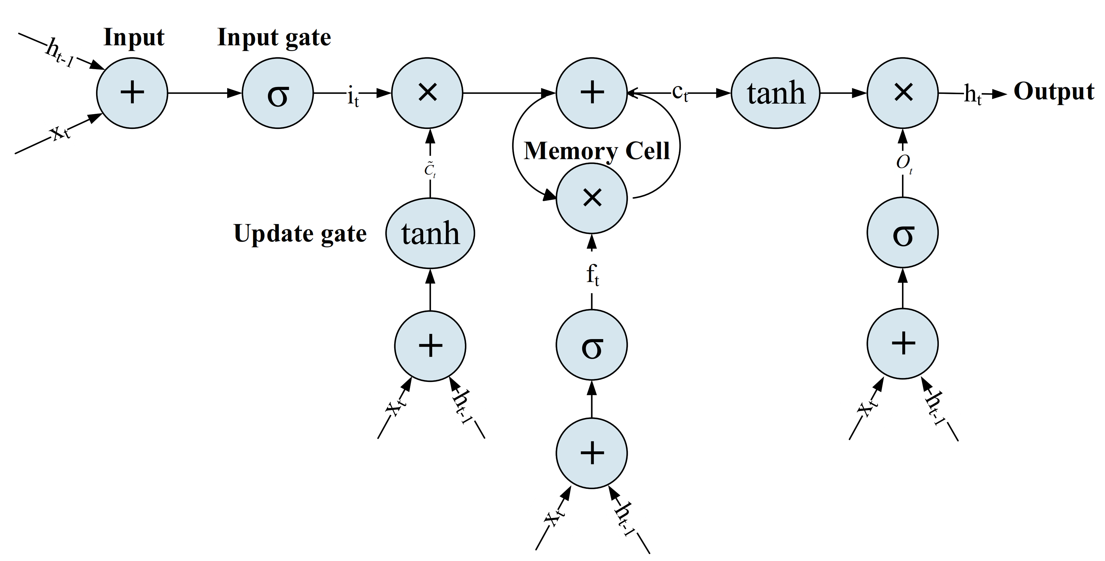
LSTM is proposed by Hochreiter and Schmidhuber [49] to learn long-term dependence information. It is a time recurrent neural network that based on recurrent neural network (RNN). RNN as the traditional neural network is different from the general neural network especially in the way of neuron connection: the information of general neural network flows unidirectional, while the information transmission of RNN has a directional loop [50]. After the improvement, the LSTM replaces the hidden layer neurons of the RNN with memory units, then it introduces “gates” to select and control discarding or adding information. Through the gate structure on the unit state, the neural network can choose to remember or forget information [51]. The control theory of the gate unit is what determines whether the data is updated or discarded, so that it can solve the problems of gradient disappearance and gradient explosion in the later stage of RNN network training. The sequence principle of LSTM is shown in Figure 1. The core calculation formula of the LSTM model is as follows [52]:

(1)

Defining the function of the input gate, forget gate, output gate respectively:

$$i_t=\sigma (W_i[h_{t-1},x_t]+b_i)$$

(17)

$$f_t=\sigma (W_f[h_{t-1},x_t]+b_f)$$

(18)

$$o_t=\sigma (W_o[h_{t-1},x_t]+b_o)$$

(19)

where $x_t$ is the input data for the current time step; $[h_{t-1},x_t]$ is a vector composed of two vectors; and $\sigma$ is the sigmoid activation function.

(2)

In the input gate, the new information will selectively recorded into the cell state. During the process, the target is the memory cell:

$${\tilde{c}}_t=\tanh (W_c[h_{t-1},x_t]+b_c)$$

(20)

$$c_t=f_t\circ c_{t-1}+i_t\circ {\tilde{c}}_t$$

(21)

where the $W_{f,i,c,o}$ and $b_{f,i,c,o}$ are the weight matrices and bias vectors respectively; $c_t$ is the memory cell; and ${\tilde{c}}_t$ is the element-by-element multiplication symbol between vectors.

(3)

In hidden layer output, the required output value can be determined, which target on $h_t$.

$$c_t=f_t\circ c_{t-1}+i_t\circ {\tilde{c}}_t$$

(22)

where $h_t$ is the hyperbolic tangent nonlinear function.

3. Case Study

The third part is data processing and empirical analysis. It uses actual data to verify the hybrid model and compares it with other single models to further verify the accuracy and stability of the hybrid model.

3.1. Wind Power Sequence Decomposition

This paper uses the measured wind power of Beijing Lumingshan Wind Power Plant from 10 May to 28 May 2016 as the research object. The data sampling interval was 5 min, and the original wind power sequence was decomposed by VMD. The original sequence is shown in Figure 2. The decomposition results are shown in Figure 3.

It can be seen from Figure 2 that the modal functions P₁ and P₂ have good regularity and obvious periodic correction. Among them, P₁ can represent the long-term change of wind power and P₂ can represent the short-term change. The modal function P₃ has the smallest average amplitude, large fluctuations, and poor regularity, which can indicate the randomness of wind power (Supplementary Materials).

3.2. Finding the Best Feature Set Using mRMR

Based on the results of wind power scenario analysis, screen out the key influencing factors of wind energy to improve the efficiency of load forecasting, which is shown in

Table 1. Key influencing factors of wind energy.

Feature	Description
ALt-n	Load at the time period t-n
TPt	Temperature at the predicted period t
APt	Air pressure at the predicted period t
HPt	Humidity at the predicted period t
WSt, WDt	Wheel height wind speed and wind direction at the predicted period t
TSt, TDt	10m wind speed and wind direction at the predicted period t
THSt, THDt	30m wind speed and wind direction at the predicted period t
FSt, FDt	50m wind speed and wind direction at the predicted period t
SSt, SDt	70m wind speed and wind direction at the predicted period t

.

After calculation, the best feature numbers of the three components P1, P2, and P3 are 12, 17, and 18. The corresponding optimal input feature sets are shown in

Table 2. Best input features of each component.

Load Component	The Best Input Feature Sets
P1	ALt-136, ALt-194, ALt-152, SSt, ALt-56, ALt-89, ALt-134, ALt-217, TPt, ALt-205, ALt-26, WSt,
P2	ALt-112, ALt-148, THDt, ALt-240, TSt, ALt-280, FSt, ALt-260, ALt-103, SDt, ALt-265, ALt-26, ALt-27, ALt-101, THSt, FDt
P3	ALt-239, ALt-50, FDt, ALt-3, ALt-52, TSt, ALt-184, THSt, ALt-178, ALt-257, FSt, ALt-26, SSt, ALt-171, ALt-158, WDt, TDt, THDt

.

3.3. Load Forecasting Based on FA-LSTM

This paper selects the data from 10 May 2016 to 27 May 2016 as the training set, and uses the remaining data from 28 May 2016 as the test set. On the basis of determining the best input feature set of each component, the firefly algorithm was used to optimize the weights and thresholds of LSTM. The test simulation environment for this paper was Python 3.7. The parameter settings of the firefly algorithm are shown in

Table 3. Parameter settings of the firefly algorithm.

Parameter Name	Description	Value
n	Number of individuals	50
k	Number of iterations	100
l0	Fluorescein initial value	5
η	Fluorescein update rate	0.5
ρ	Volatility coefficient	0.3
β	Update speed of decision domain	0.07
rs	Individual perception radius	5
L	Moving distance	0.05
Pk	Threshold of individual aggregation	5

.

During the optimization process of the firefly algorithm, the optimal individual fitness value changes as shown in Figure 4. It can be seen from Figure 4 that the firefly algorithm converges to the optimal fitness value of 0.06 after 60 evolutions in the case of a population of 50. This shows that the firefly algorithm can find the optimal parameters of the LSTM neural network at a small cost.

After the optimization of the firefly algorithm, it was determined that the parameter combination of the LSTM neural network is as follows: the number of hidden layers is 120, the time window step is 6, the number of training times is 160, and the learning rate is 0.015.

The forecasting results of the respective components are summed up to obtain the final forecasting result, as shown in Figure 5.

4. Comparison Analysis

In this section, SVM, LSTM, FA-LSTM, mRMR-FA-LSRM will be used to compare with the proposed VMD-mRMR-FA-LSTM in order to verify the forecasting performance of the model proposed in this paper.

Table 4. Parameter settings and input option of comparison models.

Comparison Model	Parameter Settings	Input Option
mRMR-FA-LSTM	Same as Section 3.3	After mRMR feature extraction: ALt-144, ALt-185, ALt-140, ALt-90, ALt-181, HPt, ALt-215, ALt-214, TPt, ALt-217, ALt-150, THDt, ALt-70, ALt-182, APt, THSt
FA-LSTM	Same as Section 3.3	ALt-1, ALt-48, ALt-96, ALt-192, ALt-240, TPt, APt, HPt, WSt, WDt, TSt, TDt, THSt, THDt, FSt, FDt, SSt, SDt
LSTM	Same as Section 3.3	ALt-1, ALt-48, ALt-96, ALt-192, ALt-240, TPt, APt, HPt, WSt,WDt, TSt, TDt, THSt, THDt, FSt, FDt, SSt, SDt
SVM	Penalty parameters:30 Width parameter of kernel function:60	ALt-1, ALt-48, ALt-96, ALt-192, ALt-240, TPt, APt, HPt, WSt, WDt, TSt, TDt, THSt, THDt, FSt, FDt, SSt, SDt

lists the parameter settings and input options of the comparison model.

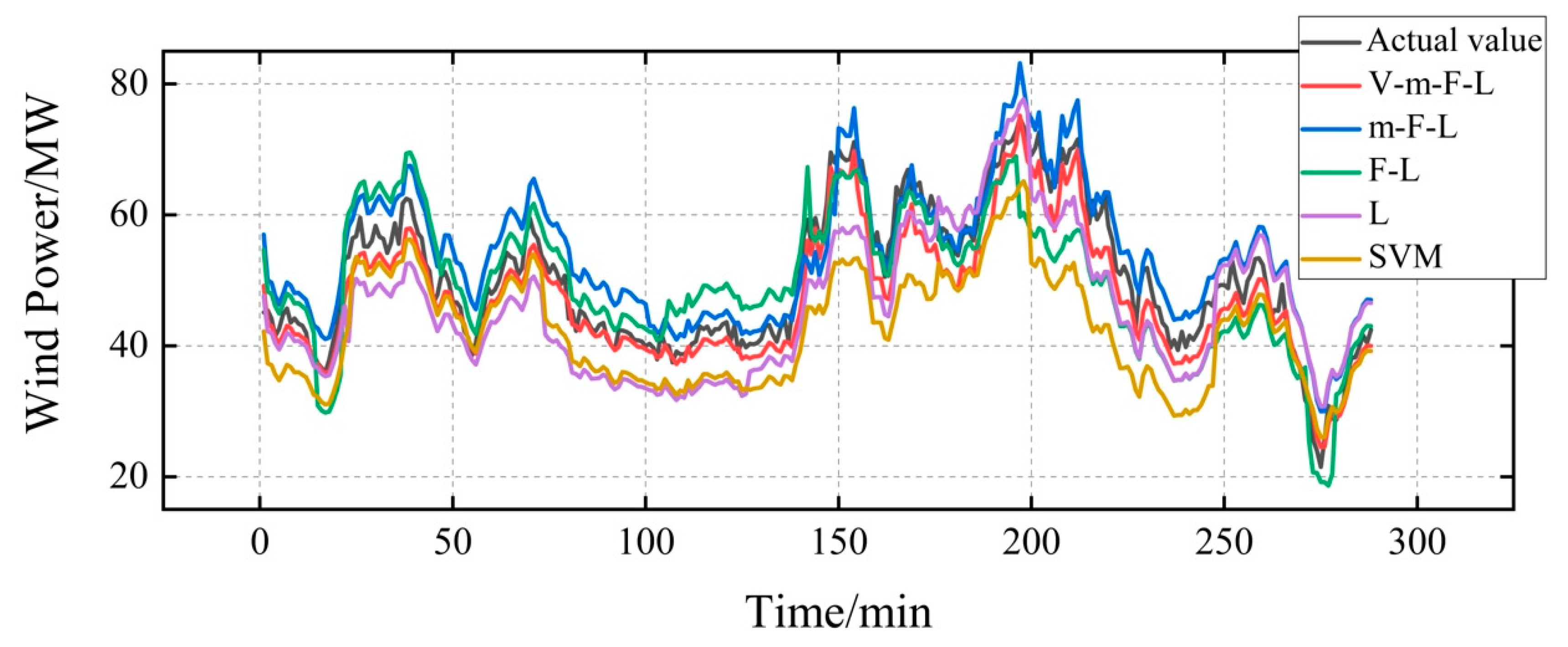
The forecasting results of each model are shown in Figure 6.

Where V-m-F-L, m-F-L, F-L, L refer to VMD-mRMR-FA-LSTM, mRMR-FA-LSTM, FA-LSTM and LSTM, respectively.

It can be seen from Figure 6 that the VMD-mRMR-FA-LSTM short-term load forecasting model can better approximate the true value and have better forecasting accuracy.

In order to quantitatively analyze the forecasting accuracy of each model, five evaluation indicators were introduced for forecasting results, that is the coefficient of determination (${\mathrm{R}}^2$), mean absolute error (MAE), mean absolute percentage error (MAPE) and root mean square error (RMSE). This can be defined as follows:

$${\mathrm{R}}^2=1-\frac{{\displaystyle \sum _{i=1}^m{(\widehat{X}(i)-X(i))}^2}}{{\displaystyle \sum _{i=1}^m{\left(X\right(i)-\overline{X}(i\left)\right)}^2}}$$

(23)

$$\mathrm{MAE}=\frac{1}{m}{\displaystyle \sum _{i=1}^m|\widehat{X}(i)-X(i)|}$$

(24)

$$\mathrm{RMSE}=\sqrt{\frac{1}{m}{\displaystyle \sum _{i=1}^m{(\widehat{X}(i)-X(i))}^2}}$$

(25)

$$\mathrm{MAPE}=\frac{1}{m}{\displaystyle \sum _{i=1}^m|\frac{\widehat{X}(i)-X(i)}{X(i)}}|\times 100\%$$

(26)

$$\mathrm{TIC}=\frac{\sqrt{\frac{1}{m}{\displaystyle \sum _{i=1}^m{(\widehat{X}(i)-X(i))}^2}}}{\sqrt{\frac{1}{m}{\displaystyle \sum _{i=1}^{m}X{(i)}^2}}+\sqrt{\frac{1}{m}{\displaystyle \sum _{i=1}^m\widehat{X}{(i)}^2}}}$$

(27)

where $m$ is the number of data points; $\overline{X}(i)=\frac{1}{m}{\displaystyle \sum _{i=1}^{m}X(i)}$. The smaller the values of RMSE, MAE, and MAPE are, the more accurate the forecasting result is. ${\mathrm{R}}^2$ can measure the regression fitting effect of the model; the larger ${\mathrm{R}}^2$ is, the better the fitting effect of the model will be. TIC can measure the predictive ability of the model.

Table 5. The comparisons of the related forecasting results for power load.

	Time(s)	${\mathbf{R}}^2$	MAE	RMSE	MAPE	TIC
VMD-mRMR-FA-LSTM	263.4638	0.9578	2.9596	3.0435	0.0569	0.0305
mRMR-FA-LSTM	193.3369	0.8958	3.2188	3.2950	0.0673	0.0311
FA-LSTM	241.3697	0.9014	3.0929	3.1483	0.0635	0.0306
LSTM	30.8964	0.7618	5.2297	4.2191	0.0979	0.0431
SVM	28.1637	0.7023	7.0238	7.4105	0.1345	0.0695

lists the comparison of ${\mathrm{R}}^2$, MAE, RMSE, MAPE, and TIC of the training results and the calculation time of each model.

Obviously, from the perspective of ${\mathrm{R}}^2$, MAE, RMSE, MAPE and TIC, the forecasting results of the model established in this paper are optimal, which are equal to 0.9578, 2.9596, 3.6435, 0.0569, and 0.0365, respectively.

Compared with mRMR-FA-LSTM, after using VMD for data decomposition, the combined model established increased by 6.9%, 8.8%, 8.3%, 18.3%, and 19.7% on the five indicators mentioned above, respectively. Compared with the FA-LSTM model, the mRMR-FA-LSTM model decreased 0.6%, 4.1%, 4.7%, 5.9%, and 1.6% on the five indicators, respectively. Comparing the FA-LSTM model and the LSTM model, it can be found that the firefly algorithm improved the forecasting results on the five indicators by 18.3%, 69.1%, 34.0%, 54.1%, and 40.8%, respectively. Comparing the LSTM model with the classic SVM model, we found that the forecasting results of LSTM improved by 8.5%, 34.3%, 75.6%, 37.4%, and 61.2% on the five indicators, respectively.

The running time of FA-LSTM and mRMR-FA-LSTM was 241.3697 s and 193.3369 s. It can be seen that in this training, the application of mRMR reduced the training time by 24.8% compared to FA-LSTM.

Finally, based on the above, we can summarize the following points:

(1)

In terms of forecasting accuracy, both the VMD decomposition and the firefly algorithm effectively improve the forecasting accuracy of the model. At the same time, LSTM has a greater advantage in wind power forecasting than the traditional SVM model. It can be found that after using mRMR for feature selection, the forecasting accuracy of FA-LSTM will slightly decrease because the indicators selected in the cases of this paper were chose based on experience.

(2)

In terms of computing efficiency, the application of mRMR, which can perform feature extraction with maximum correlation and minimum redundancy, significantly accelerates the calculation speed of the model and reduces the calculation scale, thereby improving forecasting efficiency.

(3)

After the FA algorithm is used to optimize the LSTM model, the influence of the initial value selection is reduced. The initial parameters of the model can be set more flexibly, which avoids the shortage of manual selection of model parameters.

5. Further Case Study

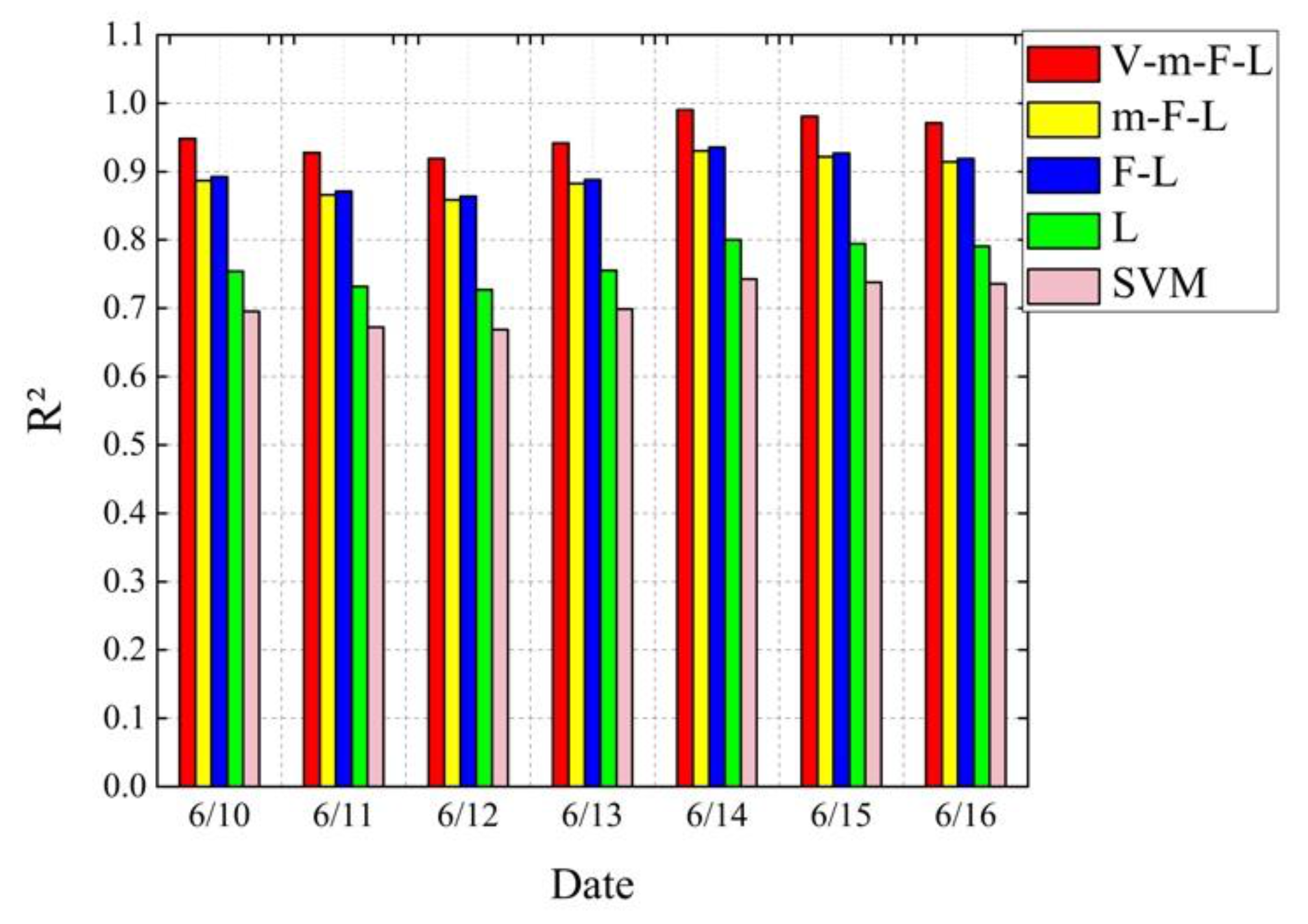
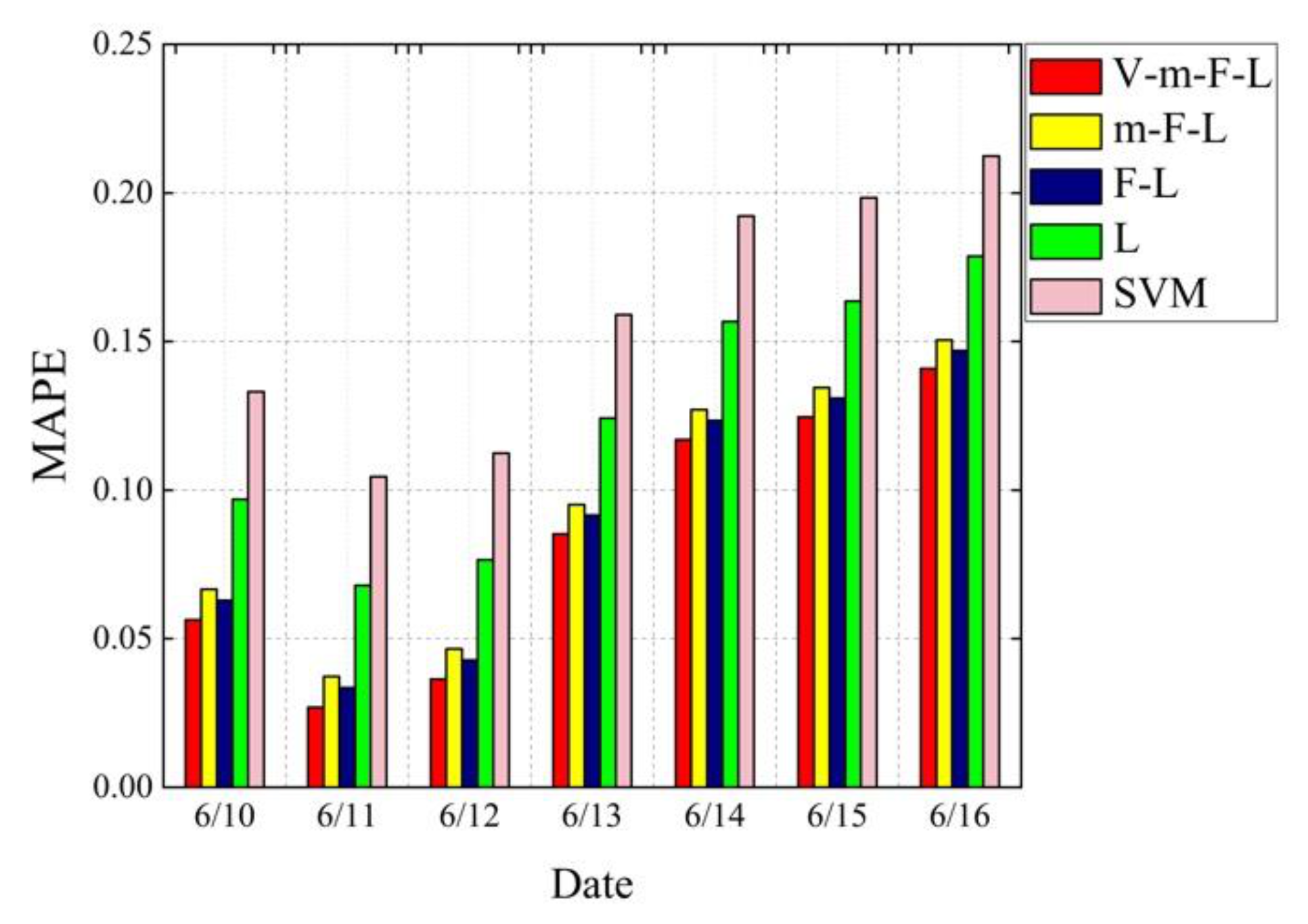
For the purpose of verifying the adaptability of the hybrid model, another case is included which selects additional load data (from 10 June 2016 to 16 June 2016) from Lumingshan Wind Power Plant. The training error of each model is shown in Figure 7, Figure 8, Figure 9, Figure 10 and Figure 11.

Noted: V-m-F-L, m-F-L, F-L, L refer to VMD-mRMR-FA-LSTM, mRMR-FA-LSTM, FA-LSTM, and LSTM, respectively.

As shown in the Figure 11, the forecasting results obtained by the model VMD-mRMR-FA-LSTM established in this paper are the best in the five parity indicators compared to the other four comparative models. It can be seen that the VMD-mRMR-FA-LSTM model can predict wind power with high accuracy.

6. Conclusions

Aiming at the instability of day-ahead wind power forecasting, a hybrid short-term wind power forecasting model, namely the VMD-mRMR-FA-LSTM model, is proposed. Firstly, the VMD decomposes the original load, and then mRMR is applied to obtain the best feature set by analyzing the correlation between each component and the features, including temperature, wind speed, wind direction, and so on. Secondly, different LSTM forecasting models for each new sequence based on the mRMR selection result are constructed. Finally, the FA is used to optimize the parameters of LSTM. The case study of the proposed hybrid model shows that:

(1) The hybrid model has higher forecasting accuracy than those of benchmarking models, and has broad application prospects in day-ahead wind power forecasting.

(2) Compared with the single LSTM model, FA can optimize the parameters and function of LSTM to obtain higher forecasting accuracy, which indicates that FA-LSTM model has stronger global search ability and more stable forecasting performance.

(3) Compared with other data preprocessing strategy, VMD-mRMR has better performance and effective improves the forecasting accuracy. The hybrid model proposed in this paper can be well applied to day-ahead wind power forecasting.

References

- National Energy Administration. China Power Industry Annual Development Report: 2019 Wind Power Grid Operation. Available online: http://www.nea.gov.cn/2020-02/28/c_138827910.htm (accessed on 28 February 2020).
- Yang, J.B.; Liu, Q.Y.; Li, X.; Cui, X.D. Overview of Wind Power in China: Status and Future. Sustainability 2017, 9, 1454. [Google Scholar] [CrossRef] [Green Version]
- Lange, M.; Focken, U. Physical Approach to Short-Term Wind Power Prediction; Springer: Berlin, Germany, 2006. [Google Scholar]
- Lahouar, A.; Slama, J.B.H. Hour-ahead wind power forecast based on random forests. Renew. Energy 2017, 109, 529–541. [Google Scholar] [CrossRef]
- Jiang, P.; Yang, H.; Heng, J. A hybrid forecasting system based on fuzzy time series and multi-objective optimization for wind speed forecasting. Appl. Energy 2019, 235, 786–801. [Google Scholar] [CrossRef]
- Heydari, A.; Nezhad, M.M.; Pirshayan, E.; Garcia, D.A.; Keynia, F.; De Santoli, L. Short-term electricity price and load forecasting in isolated power grids based on composite neural network and gravitational search optimization algorithm. Appl. Energy 2020, 277, 115503. [Google Scholar] [CrossRef]
- Zhen, H.; Niu, D.X.; Yu, M.; Wang, K.K.; Liang, Y.; Xu, X.M. A Hybrid Deep Learning Model and Comparison for Wind Power Forecasting Considering Temporal-Spatial Feature Extraction. Sustainability 2020, 12, 9490. [Google Scholar] [CrossRef]
- Chen, K.S.; Lin, K.P.; Yan, J.X.; Hsieh, W.L. Renewable Power Output Forecasting Using Least-Squares Sopport Vector Regression and Google Data. Sustainability 2019, 11, 3009. [Google Scholar] [CrossRef] [Green Version]
- Zhou, J.G.; Yu, X.C.; Jin, B.L. Short-Term Wind Power Forecasting: A New Hybrid Model Combined Extreme-Point Symmetric Mode Decomposition, Extreme Learning Machine and Particle Swarm Optimization. Sustainability 2018, 10, 3202. [Google Scholar] [CrossRef] [Green Version]
- Zhou, J.; Shi, J.; Li, G. Fine tuning support vector machines for short-term wind speed forecasting. Energy Convers. Manag. 2011, 52, 1990–1998. [Google Scholar] [CrossRef]
- Shi, X.Y.; Lei, X.W.; Huang, Q.; Huang, S.Z.; Ren, K.; Hu, Y.Y. Hourly day-ahead wind power prediction using the hybrid model of variational model decomposition and long short term memory. Energies 2018, 11, 3227. [Google Scholar] [CrossRef] [Green Version]
- Amjady, N.; Abedinia, O. Short Term Wind Power Prediction Based on Improved Kriging Interpolation, Empirical Mode Decomposition, and Closed-Loop Forecasting Engine. Sustainability 2017, 9, 2104. [Google Scholar] [CrossRef] [Green Version]
- Li, G.; Shi, J. On comparing three artificial neural networks for wind speed forecasting. Appl. Energy 2010, 87, 2313–2320. [Google Scholar] [CrossRef]
- De Giorgi, M.G.; Campilongo, S.; Ficarella, A.; Congedo, P.M. Comparison between wind power prediction models based on wavelet decomposition with least-squares support vector machine (LS-SVM) and artificial neural network (ANN). Energies 2014, 7, 5251–5272. [Google Scholar] [CrossRef]
- Liu, H.; Tian, H.Q.; Liang, X.F.; Li, Y.F. Wind speed forecasting approach using secondary decomposition algorithm and Elman neural networks. Appl. Energy 2015, 157, 183–194. [Google Scholar] [CrossRef]
- Han, L.; Jing, H.T.; Zhang, R.C.; Gao, Z.Y. Wind power forecast based on improved Long Short Term Memory network. Energy 2019, 189, 116300. [Google Scholar] [CrossRef]
- Sang, B.Y.; Wang, D.S.; Yang, B.; Ye, J.L.; Tao, Y.B. Energy storage optimal allocation method for smoothing new energy output fluctuation. Proc. CSEE 2014, 34, 3700–3706. [Google Scholar]
- Wang, C.; Zhang, H.L.; Fan, W.H.; Ma, P. A new chaotic time series hybrid prediction method of wind power based on EEMD-SE and full-parameters continued fraction. Energy 2017, 138, 977–990. [Google Scholar] [CrossRef]
- Ma, X.B. Short-term wind power prediction based on wavelet analysis and BP neutral network. J. Electr. Power Sci. Technol. 2015, 30, 92–97. [Google Scholar]
- Niu, M.F.; Hu, Y.Y.; Sun, S.L.; Liu, Y. A novel hybrid decomposition-ensemble model based on VMD and HGWO for container throughput forecasting. Appl. Math. Model. 2018, 57, 163–178. [Google Scholar] [CrossRef]
- Liang, Y.; Niu, D.X.; Hong, W.C. Short term load forecasting based on feature extraction and improved general regression neural network model. Energy 2019, 166, 653–663. [Google Scholar] [CrossRef]
- Wang, Q.; Guan, T.S.; Qin, B.S. Short-term wind speed forecasting of ORELM based on MRMR. Renew. Energy Resour. 2018, 36, 85–90. [Google Scholar]
- Bouzgou, H.; Gueymard, C.A. Minimum redundancy—Maximum relevance with extreme learning machines for global solar radiation forecasting: Toward an optimized dimensionality reduction for solar time series. Solar Energy 2017, 158, 595–609. [Google Scholar] [CrossRef]
- Zhao, H.R.; Zhao, H.R.; Guo, S. Short-Term Wind Electric Power Forecasting Using a Novel Multi-Stage Intelligent Algorithm. Sustainability 2018, 10, 881. [Google Scholar] [CrossRef] [Green Version]
- Wu, Q.L.; Lin, H.X. Short-Term Wind Speed Forecasting Based on Hybrid Variational Mode Decomposition and Least Squares Support Vector Machine Optimized by Bat Algorithm Model. Sustainability 2019, 11, 652. [Google Scholar] [CrossRef] [Green Version]
- Yang, W.; Wang, J.; Niu, T.; Du, P. A hybrid forecasting system based on a dual decomposition strategy and multi-objective optimization for electricity price forecasting. Appl. Energy 2019, 235, 1205–1225. [Google Scholar] [CrossRef]
- Sun, H.R.; Zhang, G.; Wang, R.J. Short-term wind power prediction based on combinatorial optimization algorithm. J. North China Electr. Power Univ. 2020, 47, 33–42. [Google Scholar]
- Zhao, Q.; Huang, J.T. On ultra-short-term wind power prediction based on EMD-SA-SVR. Power Syst. Prot. Control 2020, 48, 89–96. [Google Scholar]
- Zhang, Y.C.; Le, J.; Liao, X.B.; Zheng, F.; Li, Y.H. A novel combination forecasting model for wind power integrating least square support vector machine, deep belief network, singular spectrum and analysis and locality-sensitive Hashing. Energy 2019, 168, 558–630. [Google Scholar] [CrossRef]
- Wang, H.Z.; Li, G.Q.; Wang, G.B.; Peng, J.C.; Jiang, H.; Liu, Y.T. Deep learning based ensemble approach for probabilistic wind power forecasting Physical modeling methods. Appl. Energy 2016, 188, 56–70. [Google Scholar] [CrossRef]
- Wang, C.; Zhang, H.L.; Ma, P. Wind power forecasting based on singular spectrum analysis and a new hybrid Laguerre neural network. Appl. Energy 2019, 259, 114–139. [Google Scholar] [CrossRef]
- Lang, W.M.; Ma, X.J.; Zhou, B.W.; Yang, D.S.; Luo, Y.H.; Liu, L.Q. Wind power probabilistic intervals prediction based on LSTM and nonparametric kernel density Estimation. New Energy 2020, 48, 31–38. [Google Scholar]
- Liang, S.; Nguyen, L.; Jin, F. A multi-variable stacked long-short term memory network for wind speed forecasting. In IEEE international conference on big data (big data). In Proceedings of the IEEE International Conference on Big Data (Big Data) 2018, Seattle, WA, USA, 10–13 December 2018; pp. 4561–4564. [Google Scholar]
- Lopez, E.; Valle, C.; Allende, H.; Gil, E.; Madsen, H. Wind power forecasting based on echo state networks and long short-term memory. Energies 2018, 10657, 526. [Google Scholar] [CrossRef] [Green Version]
- Bao, Z.Q.; Zhao, Y.; Hu, X.T.; Zhao, Y.Y.; Huang, Q.D. Minimal peephole long short-term memory. Comput. Eng. Des. 2020, 41, 134–138. [Google Scholar]
- Flores, J.J.; Graff, M.; Rodriguez, H. Evolutive design of ARMA and ANN models for time series forecasting. Renew. Energy 2012, 44, 225–230. [Google Scholar] [CrossRef]
- Zhao, J.; Guo, Z.H.; Su, Z.Y.; Zhao, Z.Y.; Xiao, X.; Liu, F. An improved multi-step forecasting model based on WRF ensembles and creative fuzzy systems for wind speed. Appl. Energy 2016, 162, 808–826. [Google Scholar] [CrossRef]
- Wang, J.; Liu, G.Y. Firefly algorithm based on dynamic step change. Comput. Eng. Des. 2019, 40, 1001–1007. [Google Scholar]
- Ju, Z.; He, J.J. Prediction of lysine glutarylation sites by maximum relevance minimum redundancy feature selection. Anal. Biochem. 2018, 550, 1–7. [Google Scholar] [CrossRef]
- Li, H.; Zhang, R.C.; Wang, X.S.; Bao, A.C.; Jing, H.T. Multi-step wind power forecast based on VMD-LSTM. IET Renew. Power Gener. 2019, 13, 1690–1700. [Google Scholar]
- Dragomiretskiy, K.; Zosso, D. Variational Mode Decomposition. IEEE Trans. Signal Proc. 2014, 62, 531–544. [Google Scholar] [CrossRef]
- Wang, S.; Jiang, X.; Zeng, L.; Chang, Y.F. Ultra-short-term Photovoltaic Power Prediction Based on VMD-DESN-MSGP Model. Power Syst. Technol. 2020, 44, 917–926. [Google Scholar]
- Sun, Z.X.; Zhao, S.S.; Zhang, Z.X. Short-Term Wind Power Forecasting on Multiple Scales Using VMD Decomposition, K-Means Clustering and LSTM Principal Computing. IEEE Access 2019, 7, 166917–166929. [Google Scholar] [CrossRef]
- Peng, H.C.; Long, F.H.; Ding, C. Feature selection based on mutual information criteria of max-dependency and min-redundancy. IEEE Trans. Pattern Anal. Mach. Intell. 2005, 27, 1226–1238. [Google Scholar] [CrossRef] [PubMed]
- Hui, Z.; Chen, P. Oil Spills Identification in SAR Image Using mRMR and SVM Model. In Proceedings of the 2018 5th International Conference on Information Science and Control Engineering (ICISCE), Zhengzhou, China, 20–22 July 2018. [Google Scholar]
- Adil, B.-H.; Youssef, G.; Abderrahim, E.Q. HVS-MRMR wrapper method for variables selection. In Proceedings of the Second International Conference on Intelligent Systems and Computer Vision (ISCV), Fez, Morocco, 17–19 April 2017. [Google Scholar]
- Chen, H.D.; Zhuang, P.; Xia, J.K.; Dai, W.Z.; Lu, Y.; Gao, Q.; Chen, T. Optimal power flow of distribution network with distributed generation based on modified firefly algorithm. Power Syst. Prot. Control 2016, 44, 149–154. [Google Scholar]
- Wang, X.; Huang, K.; Zheng, Y.H.; Li, L.X.; Shao, F.P.; Jia, L.K.; Xu, Q.S. Combined PV Power Forecast Based on Firefly Algorithm Generalized Regression Neural Network. Power Syst. Technol. 2017, 42, 455–461. [Google Scholar]
- Rukslin; Haddin, M.; Suprajitno, A. Pitch angle controller design on the wind turbine with Permanent Magnet Synchronous Generator (PMSG) base on Firefly Algorithms (FA). In Proceedings of the 2016 International Seminar on Application for Technology of Information and Communication (ISemantic), Semarang, Indonesia, 5–6 August 2016. [Google Scholar]
- Liu, H.; Mi, X.W.; Li, Y.F. Wind speed forecasting method based on deep learning strategy using empirical wavelet transform, long short term memory neural network and Elman neural network. Energy Convers. Manag. 2018, 156, 498–514. [Google Scholar] [CrossRef]
- Cheng, R.; Jin, Y. A social learning particle swarm optimization algorithm for scalable optimization. Inf. Sci. 2015, 291, 43–60. [Google Scholar] [CrossRef]
- Li, F.L.; Chen, S.; Fan, X.J.; Liu, Y. Path Planning Based on Firefly Algorithm in Dynamic Unknown Environment. Autom. Instrum. 2019, 34, 53–58. [Google Scholar]
Figure 1.
The sequence principle of long short-term memory (LSTM).
Figure 2.
The original load sequence.
Figure 3.
(a) Modal functions P1 and (b) Modal functions P2 and (c) Modal functions P3.
Figure 4.
The fitness curve of firefly algorithm.
Figure 5.
The final forecasting results.
Figure 6.
Load forecasting curves of each model.
Figure 7.
R2 of forecasting models.
Figure 8.
MAE of forecasting models.
Figure 9.
RMSE of forecasting models.
Figure 10.
MAPE of forecasting models.
Figure 11.
TIC of forecasting models.