The Hierarchical VIKOR Method with Incomplete Information: Supplier Selection Problem

Abstract

To solve a multi-criteria decision-making problem, many attempts have been made to alleviate difficulties of obtaining precise preference information attributed to time pressure, lack of data and domain knowledge, limited attention and information processing capabilities, etc. Structuring any decision problem hierarchically is known to be an efficient way of dealing with complexity and identifying the major components of the problem. In this paper, we propose the hierarchical VIKOR method that uses incomplete alternatives’ values as well as incomplete criteria weights, extending previous works that consider mostly intervals or fuzzy under a flat structure of criteria. It ranks alternatives using the aggregated scores of group utility and individual regret scores which are computed from the linear programs. To show how to use our proposed method, we exemplified an international supplier selection problem that affects the organization’s sustainable growth.

1. Introduction

Multi-criteria decision-making (MCDM) methods provide an effective means of assisting decision-makers to select the best alternative under various criteria. Especially, incomplete information has been widely-used in MCDM problems because of the diverse difficulties the decision might need to be made under lack of time, the decision-maker might not want to provide precise data, or the decision-maker might have a limited scope of information [1,2]. The incomplete information in the literature on MCDM encompasses incomplete weights and values. Many studies about incomplete weights are found, more frequently relative to incomplete values, in MCDM literature since they often occur in practice [3,4,5,6,7,8,9,10,11]. The linear types of incomplete values may include [10,12]: (a) Strict preference, (b) weak preference, (c) weak differences of preference, (d) ratio preferences.

The VIKOR method was developed for multi-criteria optimization of complex systems [13], which focuses on ranking and selecting from a set of available alternatives in the presence of conflicting criteria [14,15]. The VIKOR method is suitable for those situations where the goal is to maximize profit while the risk of the decisions is deemed to be less important. The major advantage of the VIKOR method is that it can trade off the maximum group utility of the “majority” and the minimum individual regret of the “opponent” [14,16,17].

A number of applications have been developed in the fields of studies (e.g., material selection, water resource planning, land-use restrictions, satisfaction measuring, investment, etc.), particularly in view of organization’s sustainability under MCDM environment [18,19,20,21,22,23,24,25,26,27,28].

Fei et al. [29] proposed the DS-VIKOR method for supplier selection problem, which extends the VIKOR method by Dempster–Shafer evidence theory. Yang and Wu [30] presented the R-VIKOR method using the historical maximum and minimum data to resolve the rank reversal. Dev et al. [31] used the Entropy-VIKOR method to piston material selection problem.

In terms of information type, various forms of incomplete information (mainly fuzzy data) were dealt with in the context of the VIKOR method. Sayadi et al. [32] introduced the extended VIKOR method using interval criteria values. Opricovic [21] considered triangular fuzzy data in an application to water resources planning. Chatterjee and Chakraborty [33] analyzed the ranking performance of the original VIKOR method and its five variants, such as the comprehensive, the fuzzy, the regret theory-based, the modified, and the interval VIKOR methods. Kim and Ahn [34] proposed the VIKOR method using incomplete criteria weights under the flat structure of criteria weights. Moreover, they provided new insights that shed light on the relationship between the VIKOR and the decision-making under uncertainty (DMUU) method.

In this paper, we propose a new VIKOR method that makes use of incomplete alternatives’ values, as well as incomplete criteria weights in the hierarchically structured problem. Structuring any decision problem hierarchically is an efficient way of dealing with complexity and identifying the major components of the problem. The hierarchical structure allows management in constructing a hierarchy to fit their idiosyncratic needs [35]. A number of studies [27,36,37,38,39,40], entitled the VIKOR with fuzzy AHP, are found in the literature on the VIKOR, but they use the hierarchical structure for determining the criteria weights and then apply the classical VIKOR method to aggregate the scores. Our hierarchical VIKOR method aggregates scores in bottom-up fashion until reaching top-most node under hierarchically structured criteria. Further, we propose the hierarchical VIKOR method featuring both (a) incomplete criteria weights instead of previous entropy (objective weights), equal weights, AHP, or fuzzy (subjective weights) and (b) incomplete alternatives’ values instead of interval or fuzzy values.

The remaining of the paper is organized as follows. In Section 2, we review the VIKOR method, and then present types of incomplete alternatives’ values and their extreme points. Further, we present an information processing procedure under our hierarchical VIKOR method incorporated by incomplete alternatives’ values as well as incomplete criteria weights. A numerical example and the discussions of its results are presented in Section 3 and Section 4 respectively. Finally, the conclusion is in Section 5.

2. The Hierarchical VIKOR Method with Incomplete Information

2.1. The VIKOR Method

In MCDM problems, one usually considers a finite discrete set of alternatives $A_i$, $i=1,\dots m$, each of which is evaluated by n multiple criteria $c_j$, $j=1,\dots n$.

Table 1. Decision matrix.

	${\mathit{c}}_1$	${\mathit{c}}_2$	$\cdots$	${\mathit{c}}_{\mathit{n}}$
$A_1$	$f_{11}$	$f_{12}$	$\cdots$	$f_{1n}$
$A_2$	$f_{21}$	$f_{22}$	$\cdots$	$f_{2,}$
$⋮$	$⋮$	$⋮$	$⋮$	$⋮$
$A_m$	$f_{m1}$	$f_{m2}$	$\cdots$	$f_{mn}$

shows a decision matrix composed of the alternatives, the criteria, and the consequence $f_{ij}$ of alternative $A_i$ with respect to the criterion, $c_j$. Further, we denote a set of unknown criteria weights as $W=\{\mathrm{w}:{\displaystyle \sum }_{j=1}^n{w}_j=1, w_j\ge 0, j=1,\dots ,n\}$.

Considering the $L_p$-metric below, the VIKOR method uses both a maximum group utility based on $L_1$ and a minimum individual regret of the “opponent” based on $L_{\infty }$ (see Equations (3) and (4)).

$$L_{pi}={\left({{\displaystyle \sum }}_{j=1}^n{\left(\frac{f_j^{*}-f_{ij}}{f_j^{*}-f_j^{-}}\right)}^p\right)}^{\frac{1}{p}},1\le p<\infty ,i=1, 2,\dots , m.$$

(1)

We briefly describe the procedure of the VIKOR method in the following four steps (For convenience, we assume “more is better” criteria):

(a) Determine the best $f_j^{*}$ and the worst $f_j^{-}$ for each criterion function.

$$f_j^{*}={\max }_i{f}_{ij}, f_j^{-}={\min }_i{f}_{ij}, j=1,\dots ,n.$$

(2)

(b) Compute $S_i$ (group utility) and $R_i$ (individual regret) for each alternative.

$$S_i={{\displaystyle \sum }}_{j=1}^n{w}_j\left(f_j^{*}-f_{ij}\right)/\left(f_j^{*}-f_j^{-}\right), i=1,\dots ,m,$$

(3)

$$R_i={\max }_j{w}_j\left(f_j^{*}-f_{ij}\right)/\left(f_j^{*}-f_j^{-}\right), i=1,\dots ,m.$$

(4)

(c) Compute the value $Q_i$ for each alternative.

$$Q_i=v\frac{S_i-S^{*}}{S^{-}-S^{*}}+\left(1-v\right)\frac{R_i-R^{*}}{R^{-}-R^{*}}, i=1,\dots ,m$$

(5)

$$S^{*}={\min }_i{S}_i,S^{-}={\max }_i{S}_i,$$

(6)

$$R^{*}={\min }_i{R}_i,R^{-}={\max }_i{R}_i.$$

(7)

The constant $v$ is the weight introduced to support the strategy of maximum group utility while $\left(1-v\right)$ is used to weigh the individual regret, usually, $v=0.5$.

(d) Rank the alternatives by sorting the values $S_i$, $R_i$, and $Q_i$ in descending order. The results are three ranking lists that can be used to propose and validate a compromise solution [14].

2.2. The Incomplete Information

The incomplete information has been widely-used in MCDM problems because of various difficulties associated with information acquisition the decision might need to be made under lack of time, the decision-maker might not want to provide precise data, or the decision-maker might have limited scope of information [1,2]. We find in the literature on the VIKOR that the incomplete information has been used mostly in the form of interval or fuzzy until Kim and Ahn [34] proposed a more general form of incomplete criteria weights. Ahn [12] presented the formulas for determining the extreme points of four types of incomplete criteria weights, such as weak inequalities, strict inequalities, ratio bounds, and preference differences (see [3,4,5,6,7,8,9,10,11,12,41,42,43] for more references). The incomplete information about values could occur in practice as well. For qualitative criteria, a decision-maker may say an alternative is best (100%), and another is in the level between 80% and 90% relative to the level of the first one [44]. This can be expressed in the form of ratio bounds. Similarly to the incomplete criteria weights, the formulas for determining the extreme points of incomplete values are summarized in

Table 2. Extreme points of incomplete values.

Forms	Extreme Points
Strict preference $V_j=\{1\ge v_j\left(x_i\right)-v_j\left(x_{i+1}\right)\ge {ϵ}_i\ge 0,$ $i=1,\dots ,m-1, v_j\left(x_m\right)\ge 0$}	${\mathrm{v}}_j^1={\left(1,t_2,t_3,\dots ,t_{m-1},0\right)}^{\mathrm{T}}$, ${\mathrm{v}}_j^2={\left(1,1+t_2-t_1,t_3,\dots ,t_{m-1},0\right)}^{\mathrm{T}}$, ${\mathrm{v}}_j^3={\left(1,1+t_2-t_1,1+t_3-t_1,t_4,\dots ,t_{m-1},0\right)}^{\mathrm{T}}$, $\dots$ ${\mathrm{v}}_j^{m-1}={\left(1,1+t_2-t_1,\dots ,1+t_{m-1}-t_1,0\right)}^{\mathrm{T}}$, $(t_j={\displaystyle \sum }_{k=j}^m{ϵ}_k, j=1,\dots ,m-1$)
Weak preference $V_j=\left\{1\ge v_j\left(x_1\right)\ge v_j\left(x_2\right)\ge \dots \ge v_j\left(x_m\right)\ge 0\right\}$	${\mathrm{v}}_j^1={\left(1,0,0,\dots ,0\right)}^{\mathrm{T}}$, ${\mathrm{v}}_j^2={\left(1,1,0,\dots ,0\right)}^{\mathrm{T}}$, $\dots$ ${\mathrm{v}}_j^{m-1}={\left(1,1,1,\dots ,1,0\right)}^{\mathrm{T}}$
Weak differences in preference $V_j=\left\{1\ge v_j\left(x_1\right)-v_j\left(x_2\right)\ge \dots \ge v_j\left(x_{m-1}\right)-v_j\left(x_m\right)\ge v_j\left(x_m\right)\ge 0\right\}$	${\mathrm{v}}_j^1={\left(1,0,0,\dots ,0\right)}^{\mathrm{T}}$, ${\mathrm{v}}_j^2={\left(1,\frac{1}{2},0,\dots ,0\right)}^{\mathrm{T}}$, $\dots$ ${\mathrm{v}}_j^{m-2}={\left(1,\frac{m-3}{m-2},\dots \frac{1}{m-2},0,0\right)}^{\mathrm{T}}$, ${\mathrm{v}}_j^{m-1}={\left(1,\frac{m-2}{m-1},\dots \frac{1}{m-1},0,0\right)}^{\mathrm{T}}$
Ratio preference $V_j=\{1\ge v_j\left(x_i\right)\ge {\alpha }_i{v}_j\left(x_{i+1}\right)\ge 0,$ $i=1,\dots ,m-1, v_j\left(x_m\right)\ge 0\}$	${\mathrm{v}}_j^1={\left(1,0,0,\dots ,0\right)}^{\mathrm{T}}$, ${\mathrm{v}}_j^2={\left(1,\frac{1}{{\alpha }_1},0,\dots ,0\right)}^{\mathrm{T}}$, ${\mathrm{v}}_j^3={\left(1,\frac{1}{{\alpha }_1},\frac{1}{{\alpha }_1{\alpha }_2},0,\dots ,0,0\right)}^{\mathrm{T}}$, $\dots$ ${\mathrm{v}}_j^{m-1}={\left(1,\frac{1}{{\alpha }_1},\frac{1}{{\alpha }_1{\alpha }_2},\dots ,\frac{1}{{\alpha }_1{\alpha }_2\dots {\alpha }_{m-2}},0\right)}^{\mathrm{T}}$

.

2.3. The Hierarchical VIKOR with Incomplete Information

2.3.1. The Hierarchical Structure

Given a hierarchical problem, the decision-maker will provide his or her preference information on the values of $\left\{w_j\right\}$ and $\left\{v_j(·)\right\}$. It is assumed that both criteria weights and alternatives’ values are not known precisely and hence information is to satisfy linear constraints. To model our hierarchical VIKOR with incomplete information, we adopt the notations that Ahn et al. [44] used in the mathematical programming technique for establishing dominance between alternatives under hierarchically structured criteria:

$$\begin{array}{ll}D\left(j\right)\subset J& \mathrm{the} \mathrm{set} \mathrm{of} \mathrm{criteria} \mathrm{index} \mathrm{which} \mathrm{are} \mathrm{structured} \mathrm{immediately} \mathrm{under} \mathrm{criterion} c_j. c_0 \mathrm{is} \mathrm{the} \mathrm{topmost} \mathrm{goal}.\\ T& \mathrm{the} \mathrm{set} \mathrm{of} \mathrm{twig} \mathrm{level} \mathrm{criteria}, T=\left\{j\in J|D\left(j\right)=\varnothing \right\}.\\ W_{D\left(j\right)}& \mathrm{the} \mathrm{set} \mathrm{of} \mathrm{constraints} \mathrm{on} \mathrm{the} \mathrm{weights} w_k \mathrm{of} \mathrm{criteria} k\in D\left(j\right).\\ V_j& \mathrm{the} \mathrm{set} \mathrm{of} \mathrm{constraints} \mathrm{on} \mathrm{the} \mathrm{values} v_j(·) \mathrm{of} \mathrm{alternatives} \mathrm{for} \mathrm{each} \mathrm{criterion} j\in T.\end{array}$$

Examples of $W_{D\left(j\right)}$ and $V_j$ can be

$$W_{D\left(j\right)}=\left\{\left(w_k,w_l\right)|w_k\ge 2w_l,w_k,w_l\ge 0\right\}, k, l\in D\left(j\right),$$

$$V_k=\left\{\left(v_k\left(x\right),v_k\left(y\right)\right)|v_k\left(x\right)\ge 3v_k\left(y\right)\ge 0,0.6\le v_k\left(x\right)\le 0.8\right\}.$$

They proposed two approaches (a) weight-additive approach and (b) weight-product approach of which we adopt the former and denote the set of weights as follows:

$$W=\{\begin{array}{ll}{\displaystyle {{\displaystyle \sum }}_{j\in D\left(0\right)}}{w}_j=1& \\ \begin{array}{cc}{\displaystyle {{\displaystyle \sum }}_{k\in D\left(j\right)}}{w}_k=w_j& \mathrm{for} j\notin T\\ W_{D\left(j\right)}& \mathrm{for} j\notin T\end{array}\end{array}$$

(8)

When the criteria weights and values are incompletely known, our hierarchical VIKOR method aggregates information from bottom to top and finally rank alternatives via one of two approaches: (a) the extreme point approach and (b) the LP approach.

2.3.2. The Hierarchical VIKOR Method

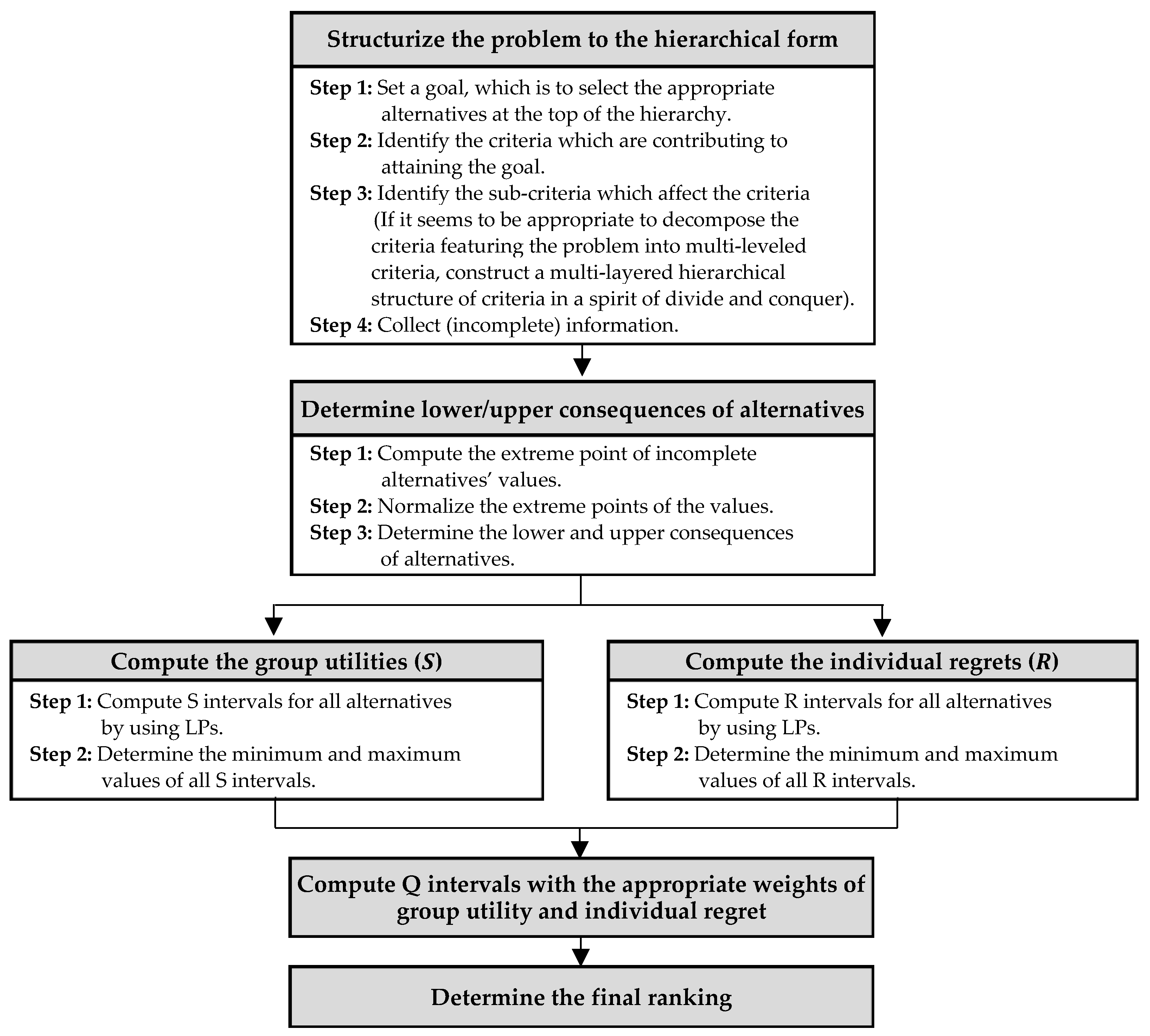
In the following, we shall describe our hierarchical VIKOR method with incomplete information in five steps, as shown in Figure 1.

Step 0.

Structurize the problem at hand to the hierarchical one when it is deemed appropriate to do so.

If it seems to be appropriate to decompose the criteria featuring the problem into multi-leveled criteria, we construct a multi-layered hierarchical structure of criteria in a spirit of divide and conquer. Required information is gathered from decision-maker in bottom-up according to the hierarchical structure.

Step 1.

Compute the extreme points of incomplete alternatives’ values and determine the lower and upper consequences of the ith alternative.

$$\left(d_1^L\left(x_i\right),\dots ,d_n^L\left(x_i\right)\right)=\left(\left(\left(1-v_1^U\left(x_i\right),\dots ,1-v_n^U\left(x_i\right)\right)|j\in \mathsf{\Psi }\right), \left(\left(v_1^L\left(x_i\right),\dots ,v_n^L\left(x_i\right)\right)|j\in \mathsf{O}\right)\right)$$

(9)

$$\left(d_1^U\left(x_i\right),\dots ,d_n^U\left(x_i\right)\right)=\left(\left(\left(1-v_1^L\left(x_i\right),\dots ,1-v_n^L\left(x_i\right)\right)|j\in \mathsf{\Psi }\right), \left(\left(v_1^U\left(x_i\right),\dots ,v_n^U\left(x_i\right)\right)|j\in \mathsf{O}\right)\right)$$

(10)

where $\mathsf{\Psi }$ and $\mathrm{O}$ are the sets of indices associated with benefit and cost criteria, respectively.

Moreover, note that $v_j^L\left(x_i\right)=\min \left(v_j\left(x_i\right)\right)$ and $v_j^U\left(x_i\right)=\max \left(v_j\left(x_i\right)\right)$ where $v_j\left(x_i\right)$ is a collection of elements associated with alternative $x_i$ in the set of extreme points of $V_j$, i.e., $v_j\left(x_i\right)=\left(v_j^1\left(x_i\right),v_j^2\left(x_i\right),\dots ,v_j^{m-1}\left(x_i\right)\right),$ $i=1,\dots ,m$, $j=1,\dots ,n$.

Step 2.

Compute S and R intervals.

In general, it is an efficient way to obtain $S$ and $R$ intervals via LPs for the hierarchical problem since the multi-leveled criteria require enormous calculations to obtain the extreme points of the criteria weights. Below are LPs for obtaining the intervals $\left[S_i^L,S_i^U\right]$ and $\left[R_i^L,R_i^U\right]$:

$$\begin{array}{lll}{S}_i^L=& \min & {{\displaystyle \sum }}_{j\in J}{d}_j^L\left(x_i\right)w_j\\ & \mathrm{s}.\mathrm{t}.& {\displaystyle \sum }_{k\in D\left(j\right)}{w}_k=w_j \mathrm{for} j\notin T,\\ & & W_{D\left(j\right)} \mathrm{for} j\notin T.\end{array}$$

(11)

$$\begin{array}{lll}{S}_i^U=& \max & {{\displaystyle \sum }}_{j\in I}{d}_j^U\left(x_i\right)w_j\\ & \mathrm{s}.\mathrm{t}.& {{\displaystyle \sum }}_{k\in D\left(j\right)}{w}_k=w_j \mathrm{for} j\notin T,\\ & & W_{D\left(j\right)} \mathrm{for} j\notin T.\end{array}$$

(12)

$$R_i^L={\min }_j\left(R_j^L\left(x_i\right)\right), R_i^U={\max }_j\left(R_j^U\left(x_i\right)\right),$$

(13)

$$\begin{array}{lll}{R}_j^L\left(x_i\right)=& \max & d_j^L\left(x_i\right)w_j\\ & \mathrm{s}.\mathrm{t}.& {{\displaystyle \sum }}_{k\in D\left(j\right)}{w}_k=w_j \mathrm{for} j\notin T,\\ & & W_{D\left(j\right)} \mathrm{for} j\notin T.\end{array}$$

(14)

$$\begin{array}{lll}{R}_j^U\left(x_i\right)=& \max & d_j^U\left(x_i\right)w_j\\ & \mathrm{s}.\mathrm{t}.& {\displaystyle \sum }_{k\in D\left(j\right)}{w}_k=w_j \mathrm{for} j\notin T,\\ & & W_{D\left(j\right)} \mathrm{for} j\notin T.\end{array}$$

(15)

Calculating $R_i\in \left[R_i^L,R_i^U\right]$ is troublesome work requiring repeated calculations and thus we modify Equations (14)–(16) by Foroughi and Aouni [45].

$$\begin{array}{lll}{R}_i^L=& \min & \beta \\ & \mathrm{s}.\mathrm{t}.& {{\displaystyle \sum }}_{k\in D\left(j\right)}{w}_k=w_j \mathrm{for} j\notin T,\\ & & W_{D\left(j\right)} \mathrm{for} j\notin T,\\ & & d_j^L\left(x_i\right)w_j-\beta \le 0, j=1,\dots ,n,\\ & & \beta \ge 0.\end{array}$$

(16)

The third constraint in Equation (16) means that $\beta \ge \max \left(d_1^L\left(x_i\right)w_1,d_2^L\left(x_i\right)w_2,\dots ,d_n^L\left(x_i\right)w_n\right)$ and thus results in the mini-max of $d_j^L\left(x_i\right)w_j$ for all $j$ in view of the objective function.

Step 3.

Compute Q intervals.

Compute the value $Q_i$ for each alternative using the relation.

$$\begin{gathered} Q_i^L=v\frac{S_i^L-S^{*}}{S^{-}-S^{*}}+\left(1-v\right)\frac{R_i^L-R^{*}}{R^{-}-R^{*}}, i=1,\dots ,m \\ {Q}_i^U=v\frac{S_i^U-S^{*}}{S^{-}-S^{*}}+\left(1-v\right)\frac{R_i^U-R^{*}}{R^{-}-R^{*}}, i=1,\dots ,m \end{gathered}$$

(17)

$$S^{*}={\min }_i{S}_i,S^{-}={\max }_i{S}_i,$$

$$R^{*}={\min }_i{R}_i,R^{-}={\max }_i{R}_i.$$

The constant $v$ is the weight introduced to support the strategy of maximum group utility while $\left(1-v\right)$ is used to weigh the individual regret, usually, $v=0.5$.

Step 4.

Determine the final ranking.

Further computations are needed to obtain the final ranking of alternatives in the face of the intervals $\left[Q_i^L,Q_i^U\right]$ in Step 3. The methods for ranking intervals can be classified into three categories. One of the most widely-used methods is to consider each location of intervals (i.e., the gaps, overlapping, etc.) and the distributions of intervals [17,41]. Xu and Da [46] presented formulas for comparing intervals based on the degree of possibility. Ahn [47] presented a method to prioritize intervals by taking into account the strength of preference based on a probabilistic measure. The similarity between two intervals can be gauged by two measures that characterize the intervals: The ratio of the overlapping portion of two intervals and the level of closeness of the midpoints between two intervals [48].

3. Numerical Example

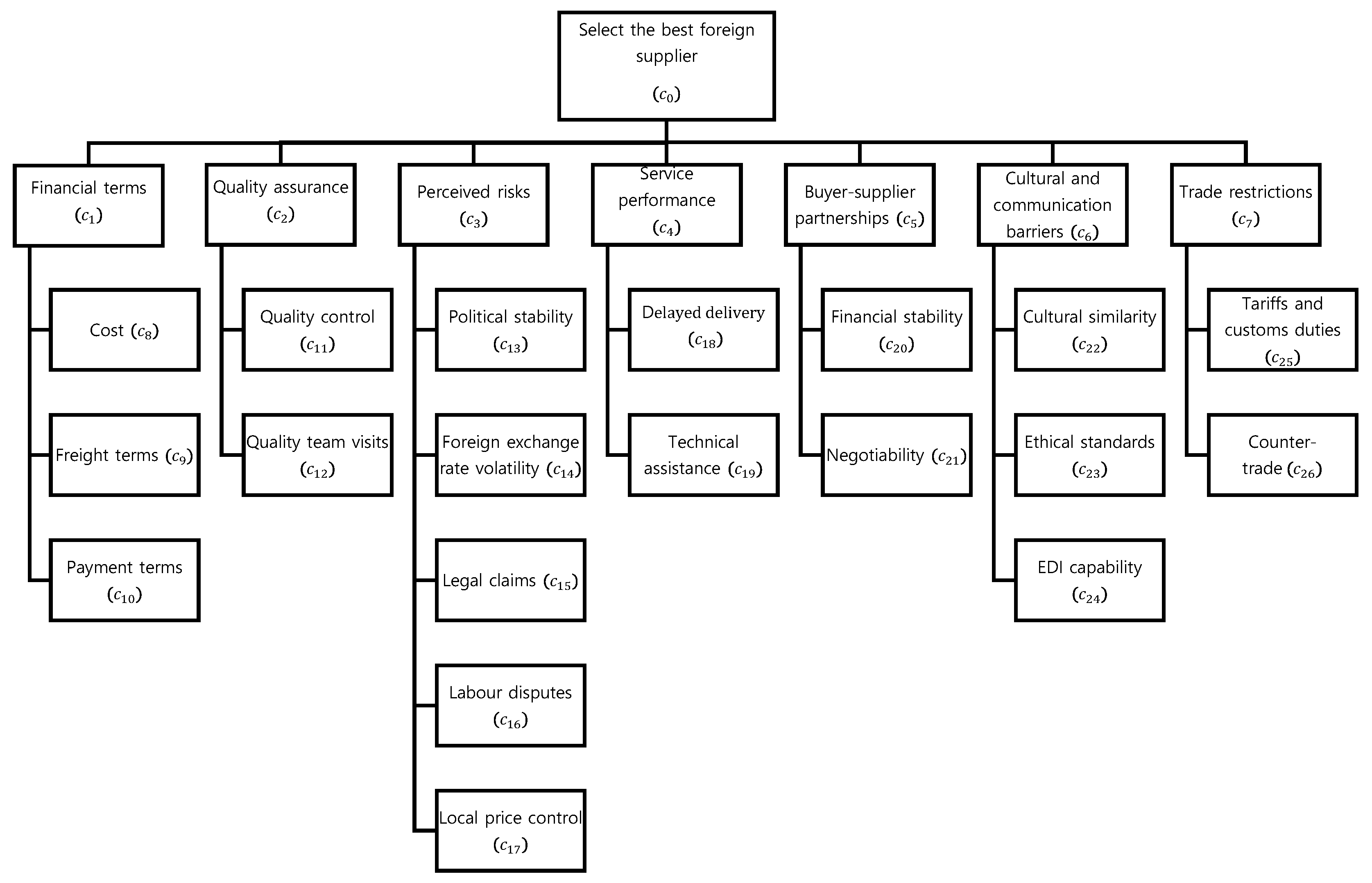
In this section, we present a numerical example to show how the proposed method can be used to solve an MCDM problem. We adopt an international supplier selection problem, which consists of a hierarchy of three levels [49], as shown in Figure 2. In an era of global sourcing, the multinational firm’s sustainable growth often hinges on the most appropriate selection of its foreign suppliers. International supplier selection, however, is very complicated and risky owing to a variety of uncontrollable and unpredictable factors affecting the decision. These factors may include political situations, tariff barriers, cultural and communication barriers, trade regulations and agreements, currency exchange rates, cultural differences, ethical standards, quality standards, etc. Nevertheless, a vast majority of the purchasing literature still focuses on the domestic aspects and neglects international supplier selection research [25].

The top level of the hierarchy represents the goal of the problem. The second level of the hierarchy contains the seven criteria (financial terms, quality assurance, perceived risks, service performance, buyer-supplier partnership, cultural and communication barriers, and trade restrictions), which are considered important in selecting the foreign supplier. Finally, the bottom level of the hierarchy is represented by sub-criteria, which are decomposed from a higher hierarchy. We consider five countries $\left(A_i, i=1,\dots ,5\right)$ as trading counterparts and the incomplete information pertinent to this supplier selection problem is given in Appendix A.

Step 1. In addition to the four types of incomplete alternatives’ values in Table 2, we include verbal expression for the criteria $c_{14}$, $c_{16}$, $c_{23}$, and $c_{25}$, and use the Bipolar scale to convert it into the interval scale [50].

We illustrate how to obtain $d_{18}^L\left(x_1\right)$ and $d_{18}^U\left(x_1\right)$ when incomplete alternatives’ values for “Delayed delivery” criterion are given as $V_{18}$,

$$V_{18}=\{1\ge v_{18}\left(A_2\right)\ge 1.5v_{18}(A_3)=1.5v_{18}\left(A_4\right)\ge 3v_{18}\left(A_1\right)\ge 4.5v_{18}\left(A_5\right)\ge 0\}.$$

The ratio information in $V_{18}$ can be interpreted as “the numbers of delayed deliveries occurred by $A_2$ is at least one and half times more than by $A_3$ and $A_4$, the numbers by $A_1$ is half less than $A_3$ and $A_4$, and finally the numbers by $A_1$ is at least one and half times more than by $A_5$ during the last decade”.

The extreme points of the set $V_{18}$ are determined by

${\mathrm{v}}_{18}^1={\left(0, 1, 0, 0,0\right)}^{\mathrm{T}}$, ${\mathrm{v}}_{18}^2={\left(0, 1, 0.6667, 0.6667, 0\right)}^{\mathrm{T}}$, ${\mathrm{v}}_{18}^3={\left(0.3333, 1, 0.6667,0.6667, 0\right)}^{\mathrm{T}}$ and $d_{18}^L\left(x_1\right)=0$, $d_{18}^U\left(x_1\right)=0.3333$.

All the values of $d_j^L\left(x_i\right)$ and $d_j^U\left(x_i\right)$ are denoted in

Table 3. The values of $d_j^L\left(x_i\right)$ and $d_j^U\left(x_i\right)$ for each alternative with respect to each criterion.

Level 1	${\mathit{c}}_{\mathbf{1}}$				${\mathit{c}}_{\mathbf{2}}$
Sub-criteria	${\mathit{c}}_{\mathbf{8}}$	${\mathit{c}}_{\mathbf{9}}$	${\mathit{c}}_{\mathbf{10}}$	${\mathit{c}}_{\mathbf{11}}$	${\mathit{c}}_{\mathbf{12}}$
$A_1$	$0$	$\left[0, 0\right]$	[0, 0]	[0, 1]	[0.4286, 0.7143]
$A_2$	$1$	$\left[1, 1\right]$	[0, 0.9]	[0, 1]	[0.1429, 0.7143]
$A_3$	$0.3913$	$\left[0, 0\right]$	[0, 0.9]	[0, 1]	[0.8571, 1]
$A_4$	$0.5652$	$\left[1, 1\right]$	[0, 1]	[0, 1]	[0.1429, 0.4296]
$A_5$	$0.2391$	$\left[1, 1\right]$	[0, 1]	[1, 1]	[0, 0.5714]
Level 1	${\mathit{c}}_{\mathbf{3}}$
Sub-criteria	${\mathit{c}}_{\mathbf{13}}$	${\mathit{c}}_{\mathbf{14}}$	${\mathit{c}}_{\mathbf{15}}$	${\mathit{c}}_{\mathbf{16}}$	${\mathit{c}}_{\mathbf{17}}$
$A_1$	$\left[1,1\right]$	$\left[0.4494, 0.6629\right]$	$\left[0.2857, 1\right]$	$\left[0.6742, 0.8876\right]$	$\left[1, 1\right]$
$A_2$	$\left[0,1\right]$	$\left[0.6742, 0.8876\right]$	$\left[0, 0.7619\right]$	$\left[0, 0.2135\right]$	$\left[0, 1\right]$
$A_3$	$\left[0,1\right]$	$\left[0.8989, 1\right]$	$\left[0.5714, 1\right]$	$\left[0.8989, 1\right]$	$\left[0, 1\right]$
$A_4$	$\left[0,1\right]$	$\left[0, 0.2135\right]$	$\left[0.8571, 0.9048\right]$	$\left[0.6742, 0.8876\right]$	$\left[0, 1\right]$
$A_5$	$\left[0,0\right]$	$\left[0.2247, 0.4494\right]$	$\left[0.5714, 0.9524\right]$	$\left[0.2247, 0.4494\right]$	$\left[0, 1\right]$
Level 1	${\mathit{c}}_{\mathbf{4}}$		${\mathit{c}}_{\mathbf{5}}$
Sub-criteria	${\mathit{c}}_{\mathbf{18}}$	${\mathit{c}}_{\mathbf{19}}$	${\mathit{c}}_{\mathbf{20}}$	${\mathit{c}}_{\mathbf{21}}$
$A_1$	$\left[0.3333, 1\right]$	$\left[1,1\right]$	$\left[1, 1\right]$	$\left[0, 0\right]$
$A_2$	$\left[1, 1\right]$	$\left[0.6667, 1\right]$	$\left[0, 1\right]$	$\left[0, 1\right]$
$A_3$	$\left[0, 0.6667\right]$	$\left[0, 0\right]$	$\left[0, 1\right]$.	$\left[0, 1\right]$
$A_4$	$\left[0, 0.6667\right]$	$\left[0.5, 1\right]$	$\left[0, 1\right]$	$\left[0, 1\right]$.
$A_5$	$\left[0,0\right]$	$\left[0.75, 1\right]$	$\left[0, 0\right]$	$\left[1, 1\right]$
Level 1	${\mathit{c}}_{\mathbf{6}}$			${\mathit{c}}_{\mathbf{7}}$
Sub-criteria	${\mathit{c}}_{\mathbf{22}}$	${\mathit{c}}_{\mathbf{23}}$	${\mathit{c}}_{\mathbf{24}}$	${\mathit{c}}_{\mathbf{25}}$	${\mathit{c}}_{\mathbf{26}}$
$A_1$	$\left[0, 1\right]$	$\left[0.2532, 0.4937\right]$	$\left[1, 1\right]$	$\left[0, 0.2405\right]$	$\left[1, 1\right]$
$A_2$	$\left[0, 1\right]$	$\left[0, 0.2405\right]$	$\left[0, 1\right]$	$\left[0, 0.2405\right]$	$\left[0, 1\right]$
$A_3$	$\left[0, 1\right]$	$\left[0.7595, 1\right]$	$\left[0, 0\right]$	$\left[0.7595, 1\right]$	$\left[0, 0\right]$
$A_4$	$\left[1, 1\right]$	$\left[0.2532, 0.4937\right]$	$\left[0, 1\right]$	$\left[0, 0.2405\right]$	$\left[0, 0\right]$
$A_5$	$\left[0, 0\right]$	$\left[0.2532, 0.4937\right]$	$\left[0, 1\right]$	$\left[0.5063, 0.7468\right]$	$\left[0, 1\right]$

.

Step 2. Compute the intervals of $\left[S_i^L,S_i^U\right]$ and $\left[R_i^L,R_i^U\right]$, using Equations (11)–(16). We show how to compute the intervals $\left[S_1^L,S_1^U\right]$ and $\left[R_1^L,R_1^U\right]$ for $A_1$ for illustrative purposes:

$$\begin{array}{lll}{\mathrm{S}}_1^L=& \min & 0.4286w_{12}+w_{13}+0.4494w_{14}+0.2857w_{15}+0.6742w_{16}+w_{17}+0.3333w_{18}\\ & & +w_{19}+w_{20}+0.2532w_{23}+w_{24}+w_{26}\end{array}$$

$$\begin{array}{ll}\mathrm{s}.\mathrm{t}.& w_j={{\displaystyle \sum }}_{k\in D\left(j\right)}{w}_k, j=1,\dots ,7\\ & W_{D\left(j\right)}, j=0,\dots ,7\end{array}$$

(18)

$$\begin{array}{lll}{\mathrm{S}}_1^U=& \max & w_{11}+0.7143w_{12}+w_{13}+0.6629w_{14}+w_{15}+0.8876w_{16}+w_{17}+w_{18}+w_{19}\\ & & +w_{20}+w_{22}+0.4937w_{23}+w_{24}+0.5714w_{25}+w_{26}\end{array}$$

$$\begin{array}{ll}\mathrm{s}.\mathrm{t}.& w_j={{\displaystyle \sum }}_{k\in D\left(j\right)}{w}_k, j=1,\dots ,7\\ & W_{D\left(j\right)}, j=0,\dots ,7\end{array}$$

(19)

$$\begin{array}{lll}{\mathrm{R}}_1^L=& \min & \beta \\ & \mathrm{s}.\mathrm{t}.& w_j={{\displaystyle \sum }}_{k\in D\left(j\right)}{w}_k, j=1,\dots ,7\\ & & W_{D\left(j\right)}, j=0,\dots ,7\\ & & w_i\le \beta , i=8,\dots ,26,\\ & & \beta \ge 0.\end{array}$$

(20)

The optimal solutions to the Equations (18)–(20) are $\left[S_1^L,S_1^U\right]=\left[0, 0.8571\right]$ and $R_1^L=0$.

We can also obtain $R_1^U$ as follows:

$R_1^U={\max }_j\left(R_j^U\left(x_1\right)\right)$

$=\max \left(0,0,0,0.5,0.18,0.33,0.09,0.08,0.15,0.07,0.25,0.13,0.2,0,0.06,0.04,0.17,0.08,0.07\right)$

$=0.5$

For example,

$$\begin{array}{lll}{R}_{12}^U\left(x_1\right)=& \max & 0.1743w_{12}\\ & \mathrm{s}.\mathrm{t}.& {{\displaystyle \sum }}_{k\in D\left(j\right)}{w}_k=w_j, j=1,\dots ,7\\ & & W_{D\left(j\right)}, j=0,\dots ,7.\end{array}$$

(21)

Step 3. Compute the intervals of $\left[Q_i^L,Q_i^U\right], i=1,\dots ,5$. We illustrate $\left[Q_1^L,Q_1^U\right]$ for alternative $A_1$ with $\mathsf{\alpha }=0.5$.

$$S^{*}=0, S^{-}=1,$$

$$R^{*}=0, R^{-}=1,$$

$$Q_1^L=\frac{0.5\left(0-0\right)}{1-0}+\frac{0.5\left(0-0\right)}{1-0}=0,$$

$$Q_1^U=\frac{0.5\left(0.8571-0\right)}{1-0}+\frac{0.5\left(0.5-0\right)}{1-0}=0.6786.$$

The intervals $\left[S_i^L,S_i^U\right]$, $\left[R_i^L,R_i^U\right]$, $\left[Q_i^L,Q_i^U\right]$, and the midpoint of $\left[Q_i^L,Q_i^U\right]$ for all alternatives are listed in

Table 4. S, R, and Q intervals with $v=0.5$.

	S Interval		R Interval		Q Interval
	${\mathit{S}}_{\mathit{i}}^{\mathit{L}}$	${\mathit{S}}_{\mathit{i}}^{\mathit{U}}$	${\mathit{R}}_{\mathit{i}}^{\mathit{L}}$	${\mathit{R}}_{\mathit{i}}^{\mathit{U}}$	${\mathit{Q}}_{\mathit{i}}^{\mathit{L}}$	${\mathit{Q}}_{\mathit{i}}^{\mathit{U}}$	${\mathit{Q}}_{\mathit{i}}^{\mathit{M}}$
$A_1$	$0$	$0.8571$	$0$	$0.5$	$0$	$0.6786$	$0.3393$
$A_2$	$0.2143$	$1$	$0.0588$	$1$	0.1366	$1$	$0.5683$
$A_3$	$0.0186$	$0.8261$	$0.0186$	$0.5$	$0.0186$	$0.6631$	$0.3408$
$A_4$	$0.0745$	$0.9517$	$0.0379$	$0.5652$	$0.0562$	$0.7585$	$0.4073$
$A_5$	$0.1056$	$0.8732$	$0.055$	$0.5$	$0.0803$	$0.6866$	$0.3834$

.

Step 4. According to the midpoints $\left(Q_i^M\right)$ in the last column in Table 4, the final ranking of alternatives is determined by $A_1>A_3>A_5>A_4>A_2$. Other methods to rank intervals are discussed in Section 4.

4. Discussion

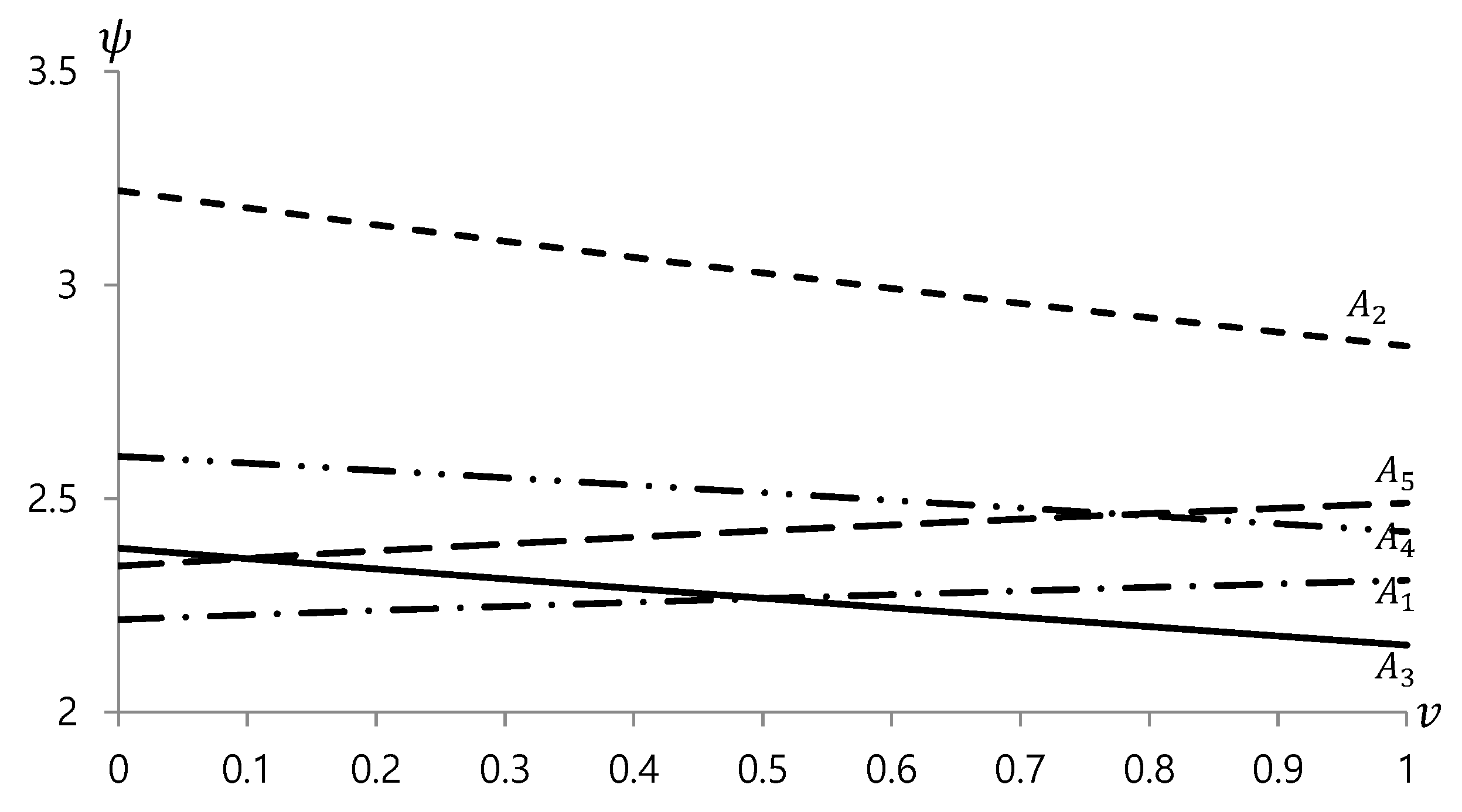
In this section, we look into how sensitive the ranking of alternatives is on the values of $v$, $0\le v\le 1$ in (17) representing relative importance of group utilities to individual regrets. This is because different values of $v$, in due course, result in different $Q$ intervals, which consequently can yield other rankings of alternatives. In fact, the midpoint approach dealt with in Step 4 of Section 3 fails to take into account useful information, such as, for example, distributions of intervals [17,41], degree of possibility [46,47], and the ratio of the overlapping portion and the level of closeness of the midpoints of the intervals [48].

As before, the values $Q_i\in \left[Q_i^L,Q_i^U\right]$ and $Q_j\in \left[Q_j^L,Q_j^U\right]$ are the aggregated intervals of group utilities and individual regrets for alternatives $A_i$ and $A_j$ for a given value of $v$. Then the degree of possibility of $Q_i$ over $Q_j$ (i.e., $A_i$ over $A_j$) is defined as

$p_{ij}=\max \left\{1-\max \left\{\frac{Q_j^U-Q_i^L}{\left(Q_i^U-Q_i^L\right)+\left(Q_j^U-Q_j^L\right)},0\right\},0\right\}$ where $p_{ij}\ge 0, p_{ij}+p_{ji}=1, p_{ii}=0.5$.

The degree of possibility of $A_i$ over the other alternatives is computed by

${\psi }_i={\displaystyle \sum }_{j=1}^n{p}_{ij}, i=1,\dots ,n.$

Applying the measure ${\psi }_i$ to $Q_i$ intervals in Table 4 leads to ${\psi }_1=2.2666, {\psi }_2=3.0279,{\psi }_3=2.2669, {\psi }_4=2.5141, {\psi }_5=2.4245$ to obtain a ranking of alternatives $A_1\ge A_3\ge A_5\ge A_4\ge A_2$. Note that this ranking is obtained based on the ascending order of $\psi$ and $v=0.5$.

Table 5. The degree of possibility of each alternative over others depending on the values of $v$.

	$\mathit{v}$
	0	0.1	0.2	0.3	0.4	0.5	0.6	0.7	0.8	0.9	1
${\psi }_1$	2.2173	2.2279	2.2381	2.248	2.2574	2.2666	2.2756	2.2843	2.2927	2.3009	2.3087
${\psi }_2$	3.2207	3.1801	3.1406	3.1021	3.0645	3.0279	2.9921	2.9571	2.923	2.8898	2.8571
${\psi }_3$	2.3846	2.3598	2.3358	2.3124	2.2895	2.2669	2.2446	2.2225	2.2007	2.1789	2.1573
${\psi }_4$	2.5992	2.5829	2.5661	2.549	2.5317	2.5141	2.4963	2.4783	2.4599	2.4414	2.4229
${\psi }_5$	2.3423	2.3606	2.3779	2.3941	2.4097	2.4245	2.4386	2.4522	2.4652	2.4777	2.4899
Ranking	*	**	**	**	**	**	***	***	****	****	****

* A₁ ≥ A₅ ≥ A₃ ≥ A₄ ≥ A₂; ** A₁≥ A₃ ≥A₅ ≥A₄ ≥ A₂; *** A₃ ≥ A₁ ≥ A₅ ≥ A₄ ≥ A₂; **** A₃ ≥A₁ ≥A₄ ≥ A₅ ≥ A₂

below lists the degree of possibility of each alternative over the other alternatives, depending on various $v$ and its resulting ranking of alternatives.

Four different rankings can be derived from Figure 3. First, the ranking of $A_1\ge A_5\ge A_3\ge A_4\ge A_2$ is obtained when the decision-maker does not emphasize the group utility at all $\left(v=0\right)$. We have the ranking of $A_1\ge A_3\ge A_5\ge A_4\ge A_2$ in case of $0.1\le v\le 0.5$. If the decision-maker stresses the group utility slightly more$\left(0.6\le v\le 0.7\right)$ or extremely $\left(0.8\le v\le 1\right)$ over the individual regret, we find that only the rank order of alternatives $A_4$ and $A_5$ changes, thus resulting in $A_3\ge A_1\ge A_5\ge A_4\ge A_2$ and $A_3\ge A_1\ge A_4\ge A_5\ge A_2$, respectively.

5. Conclusions

Expressing a set of criteria hierarchically is a natural way in the process of decomposing composite criteria into their subordinate sub-criteria (if necessary, sub-sub criteria). Further, information regarding the criteria weights can be more easily obtained by comparing criteria versus criteria of the same layer in the hierarchical structure. A number of studies were presented in the literature, mostly entitled the VIKOR method with analytic hierarchy process (AHP) to benefit from such a hierarchical representation. Unfortunately, however, we find that the VIKOR method and hierarchical structure of criteria are used separately (to say rigorously, independently) in a sense that the hierarchical structure of criteria is used in determining the criteria weights to be fed into the conventional VIKOR. In this paper, we attempted to embody a true hierarchical VIKOR method by solving the MCDM problems in two steps: (1) Represent the MCDM problems hierarchically in top-down fashion and (2) aggregate information in bottom-up fashion.

The increasing complexity of the socio-economic environments makes it less and less possible for a single decision-maker to consider all relevant aspects of a decision problem. Therefore, many organizations employ a number of experts who exhibit their own domain knowledge. Our hierarchical VIKOR method in the paper is originally designed to solve a single decision-maker’s problem and thus it is needed to cover a group decision-making problem frequently faced in the real world. With regard to this, we have to consider some strategies about how to aggregate individual preferences. In the first option, many efforts are made to communicate and negotiate among a group of members to narrow down their diverse preferences to a single aggregated preference. If this is successful, we directly apply our hierarchical VIKOR method. Otherwise, we solve individual decision-making problems (using our hierarchical VIKOR method) as many times as the number of decision-makers involved and finally attempt to aggregate individual decision outcomes expressed by the intervals of group utilities and individual regrets. Further, detailed development is left for future study.

References

- Weber, M. A method of multiattribute decision making with incomplete information. Manag. Sci. 1985, 31, 1365–1371. [Google Scholar] [CrossRef]
- Weber, M. Decision making with incomplete information. Eur. J. Oper. Res. 1987, 28, 44–57. [Google Scholar] [CrossRef]
- Ahn, B.S.; Park, K.S. Comparing methods for multiattribute decision making with ordinal weights. Comput. Oper. Res. 2008, 35, 1660–1670. [Google Scholar] [CrossRef]
- Eum, Y.S.; Park, K.S.; Kim, S.H. Establishing dominance and potential optimality in multi-criteria analysis with imprecise weight and value. Comput. Oper. Res. 2001, 28, 397–409. [Google Scholar] [CrossRef]
- Kirkwood, C.W.; Sarin, R.K. Ranking with partial information: A method and an application. Oper. Res. 1985, 33, 38–48. [Google Scholar] [CrossRef]
- Lee, K.S.; Park, K.S.; Kim, S.H. Dominance, potential optimality, imprecise information, and hierarchical structure in multi-criteria analysis. Comput. Oper. Res. 2002, 29, 1267–1281. [Google Scholar] [CrossRef]
- Mateos, A.; Jiménez, A.; Blanco, J.F. Dominance measuring method performance under incomplete information about weights. J. Multi-Criteria Decis. Anal. 2012, 19, 129–142. [Google Scholar] [CrossRef] [Green Version]
- Mateos, A.; Jiménez, A.; Ríos-Insua, S. Monte Carlo simulation techniques for group decision making with incomplete information. Eur. J. Oper. Res. 2006, 174, 1842–1864. [Google Scholar] [CrossRef]
- Mateos, A.; Ríos-Insua, S.; Jiménez, A. Dominance, potential optimality and alternative ranking in imprecise multi-attribute decision making. J. Oper. Res. Soc. 2007, 58, 326–336. [Google Scholar] [CrossRef]
- Park, K.S. Mathematical programming models for characterizing dominance and potential optimality when multicriteria alternative values and weights are simultaneously incomplete. IEEE Trans. Syst. Man Cybern. (Part A) 2004, 34, 601–614. [Google Scholar] [CrossRef]
- Puerto, J.; Mármol, A.M.; Monroy, L.; Fernández, F.R. Decision criteria with partial information. Int. Trans. Oper. Res. 2000, 7, 51–65. [Google Scholar] [CrossRef]
- Ahn, B.S. Extreme point-based multi-attribute decision analysis with incomplete information. Eur. J. Oper. Res. 2015, 240, 748–755. [Google Scholar] [CrossRef]
- Opricovic, S. Multicriteria optimization of civil engineering systems. Tech. Rep. Belgrade 1998, 2, 5–21. [Google Scholar]
- Opricovic, S.; Tzeng, G.H. Compromise solution by MCDM methods: A comparative analysis of VIKOR and TOPSIS. Eur. J. Oper. Res. 2004, 156, 445–455. [Google Scholar] [CrossRef]
- Opricovic, S.; Tzeng, G.H. Extended VIKOR method in comparison with outranking methods. Eur. J. Oper. Res. 2007, 178, 514–529. [Google Scholar] [CrossRef]
- Tavana, M.; Mavi, R.K.; Santos-Arteaga, F.J.; Doust, E.R. An extended VIKOR method using stochastic data and subjective judgments. Comput. Ind. Eng. 2016, 97, 240–247. [Google Scholar] [CrossRef]
- Wan, S.P.; Wang, Q.Y.; Dong, J.Y. The extended VIKOR method for multi-attribute group decision making with triangular intuitionistic fuzzy numbers. Knowl. Based Syst. 2013, 52, 65–77. [Google Scholar] [CrossRef]
- Bahraminasab, M.; Jahan, A. Material selection for femoral component of total knee replacement using comprehensive VIKOR. Mater. Des. 2011, 32, 4471–4477. [Google Scholar] [CrossRef]
- Chang, C.L.; Hsu, C.H. Multi-criteria analysis via the VIKOR method for prioritizing land-use restraint strategies in the Tseng-Wen reservoir watershed. J. Environ. Manag. 2009, 90, 3226–3230. [Google Scholar] [CrossRef]
- Kang, D.; Park, Y. Review-based measurement of customer satisfaction in mobile service: Sentiment analysis and VIKOR approach. Expert Syst. Appl. 2014, 41, 1041–1050. [Google Scholar] [CrossRef]
- Opricovic, S. Fuzzy VIKOR with an application to water resources planning. Expert Syst. Appl. 2011, 38, 12983–12990. [Google Scholar] [CrossRef]
- San Cristóbal, J.R. Multi-criteria decision-making in the selection of a renewable energy project in Spain: The VIKOR method. Renew. Energy 2011, 36, 498–502. [Google Scholar] [CrossRef]
- Tong, L.I.; Chen, C.C.; Wang, C.H. Optimization of multi-response processes using the VIKOR method. Int. J. Adv. Manuf. Technol. 2007, 31, 1049–1057. [Google Scholar] [CrossRef]
- Pang, N.; Guo, W. Uncertain Hybrid Multiple attribute group decision of offshore wind power transmission mode based on the VIKOR method. Sustainability 2019, 11, 6183. [Google Scholar] [CrossRef] [Green Version]
- Pérez-Velázquez, A.; Oro-Carralero, L.L.; Moya-Rodríguez, J.L. Supplier selection for photovoltaic module installation utilizing fuzzy inference and the VIKOR method: A green approach. Sustainability 2020, 12, 2242. [Google Scholar] [CrossRef] [Green Version]
- Phochanikorn, P.; Tan, C. A new extension to a multi-criteria decision-making model for sustainable supplier selection under an intuitionistic fuzzy environment. Sustainability 2019, 11, 5413. [Google Scholar] [CrossRef] [Green Version]
- Salimi, A.H.; Noori, A.; Bonakdari, H.; Masoompour Samakosh, J.; Sharifi, E.; Hassanvand, M.; Gharabaghi, B.; Agharazi, M. Exploring the role of advertising types on improving the water consumption behavior: An application of integrated fuzzy AHP and fuzzy VIKOR method. Sustainability 2020, 12, 1232. [Google Scholar] [CrossRef] [Green Version]
- Volkov, A.; Morkunas, M.; Balezentis, T.; Šapolaitė, V. Economic and environmental performance of the agricultural sectors of the selected EU countries. Sustainability 2020, 12, 1210. [Google Scholar] [CrossRef] [Green Version]
- Fei, L.; Deng, Y.; Hu, Y. DS-VIKOR: A new multi-criteria decision-making method for supplier selection. Int. J. Fuzzy Syst. 2019, 21, 157–175. [Google Scholar] [CrossRef]
- Yang, W.; Wu, Y. A new improvement method to avoid rank reversal in VIKOR. IEEE Access 2020, 8, 21261–21271. [Google Scholar] [CrossRef]
- Dev, S.; Aherwar, A.; Patnaik, A. Material selection for automotive piston component using entropy-VIKOR method. Silicon 2020, 12, 155–169. [Google Scholar] [CrossRef]
- Sayadi, M.K.; Heydari, M.; Shahanaghi, K. Extension of VIKOR method for decision making problem with interval numbers. Appl. Math. Model. 2009, 33, 2257–2262. [Google Scholar] [CrossRef]
- Chatterjee, P.; Chakraborty, S. A comparative analysis of VIKOR method and its variants. Decis. Sci. Lett. 2016, 5, 469–486. [Google Scholar] [CrossRef]
- Kim, J.H.; Ahn, B.S. Extended VIKOR method using incomplete criteria weights. Expert Syst. Appl. 2019, 126, 124–132. [Google Scholar] [CrossRef]
- Wind, Y.; Saaty, T.L. Marketing applications of the analytic hierarchy process. Manag. Sci. 1980, 26, 641–658. [Google Scholar] [CrossRef]
- Ansari, A.J.; Ashraf, I.; Gopal, B. Integrated fuzzy VIKOR and AHP methodology for selection of distributed electricity generation through renewable energy in India. Int. J. Eng. Res. Appl. 2011, 1, 1110–1113. [Google Scholar]
- Fu, H.P.; Chu, K.K.; Chao, P.; Lee, H.H.; Liao, Y.C. Using fuzzy AHP and VIKOR for benchmarking analysis in the hotel industry. Serv. Ind. J. 2011, 31, 2373–2389. [Google Scholar] [CrossRef]
- Mohaghar, A.; Fathi, M.R.; Zarchi, M.K.; Omidian, A. A combined VIKOR-fuzzy AHP approach to marketing strategy selection. Bus. Manag. Strategy 2012, 3, 13. [Google Scholar] [CrossRef] [Green Version]
- Singh, S.; Olugu, E.U.; Musa, S.N.; Mahat, A.B.; Wong, K.Y. Strategy selection for sustainable manufacturing with integrated AHP-VIKOR method under interval-valued fuzzy environment. Int. J. Adv. Manuf. Technol. 2016, 84, 547–563. [Google Scholar] [CrossRef]
- Shokri, H.; Ashjari, B.; Saberi, M.; Yoon, J.H. An integrated AHP-VIKOR methodology for facility layout design. Ind. Eng. Manag. Syst. 2013, 12, 389–405. [Google Scholar] [CrossRef] [Green Version]
- Mármol, A.M.; Puerto, J.; Fernández, F.R. The use of partial information on weights in multicriteria decision problems. J. Multi-Criteria Decis. Anal. 1998, 7, 322–329. [Google Scholar] [CrossRef]
- Mármol, A.M.; Puerto, J.; Fernández, F.R. Sequential incorporation of imprecise information in multiple criteria decision processes. Eur. J. Oper. Res. 2002, 137, 123–133. [Google Scholar] [CrossRef]
- Sarabando, P.; Dias, L.C. Simple procedures of choice in multicriteria problems without precise information about the alternatives’ values. Comput. Oper. Res. 2010, 37, 2239–2247. [Google Scholar] [CrossRef] [Green Version]
- Ahn, B.S.; Park, K.S.; Han, C.H.; Kim, J.K. Multi-attribute decision aid under incomplete information and hierarchical structure. Eur. J. Oper. Res. 2000, 125, 431–439. [Google Scholar] [CrossRef]
- Foroughi, A.A.; Aouni, B. New approaches for determining a common set of weights for a voting system. Int. Trans. Oper. Res. 2012, 19, 521–530. [Google Scholar] [CrossRef]
- Xu, Z.S.; Da, Q.L. The uncertain OWA operator. Int. J. Intell. Syst. 2002, 17, 569–575. [Google Scholar] [CrossRef]
- Ahn, B.S. The uncertain OWA aggregation with weighting functions having a constant level of orness. Int. J. Intell. Syst. 2006, 21, 469–483. [Google Scholar] [CrossRef]
- Choi, S.H.; Kang, S.; Jeon, Y.J. Personalized recommendation system based on product specification values. Expert Syst. Appl. 2006, 31, 607–616. [Google Scholar] [CrossRef]
- Min, H. International supplier selection: A multi-attribute utility approach. Int. J. Phys. Distrib. Logist. Manag. 1994, 24, 24–33. [Google Scholar] [CrossRef]
- Hwang, C.L.; Yoon, K. Multiple Attributes Decision Making Methods and Applications; Springer: Berlin, Germany, 1981. [Google Scholar]
Figure 1.
Flowchart of the hierarchical VIKOR method with incomplete information.
Figure 2.
An example of a hierarchy of criteria.
Figure 3.
The rankings of alternatives based on the values of .