Article

Optimal Placement and Sizing of Wind Generators in AC Grids Considering Reactive Power Capability and Wind Speed Curves

by
Walter Gil-González
1,
Oscar Danilo Montoya
1,2,
Luis Fernando Grisales-Noreña
3,
Alberto-Jesus Perea-Moreno
4 and
Quetzalcoatl Hernandez-Escobedo
5,*
1
Laboratorio Inteligente de Energía, Universidad Tecnológica de Bolívar, km 1 vía Turbaco, Cartagena 131001, Colombia
2
Facultad de Ingeniería, Universidad Distrital Francisco José de Caldas, Carrera 7 No. 40B-53, Bogotá D.C. 11021, Colombia
3
Grupo GIIEN, Facultad de Ingeniería, Institución Universitaria Pascual Bravo, Campus Robledo, Medellín 050036, Colombia
4
Departamento de Física Aplicada, Universidad de Córdoba, ceiA3, Campus de Rabanales, 14071 Córdoba, Spain
5
Escuela Nacional de Estudios Superiores, Campus Juriquilla, UNAM, Queretaro 3001, Mexico
*
Author to whom correspondence should be addressed.
Sustainability 2020, 12(7), 2983; https://doi.org/10.3390/su12072983
Submission received: 10 March 2020 / Revised: 28 March 2020 / Accepted: 2 April 2020 / Published: 8 April 2020
(This article belongs to the Special Issue Renewable Energy and Energy Saving: Worldwide Research Trends)

Abstract

:
This paper presents an optimization model for the optimal placement and sizing of wind turbines, considering their reactive power capacity, wind speed, and demand curves. The optimization model is nonlinear and is focused on minimizing power losses in AC distribution networks. Also, paired wind turbine and power conversion systems are treated via chargeability factor η at the peak hour. This factor represents the percentage of usage of the power conversion system in the nominal wind speed conditions, and allows to support reactive power dynamically during all periods of the day as a function of the distribution system requirements. In addition, an artificial neural network is used for short-term forecasting to deal with uncertainties in wind power generation. We assume that the number of wind power distributed generators could be from zero to three generators integrated into the system, considering unit power factors and reactive power injections to follow up the effect of reactive power compensation in the daily operation. The General Algebraic Modeling System (GAMS) is employed to solve the proposed optimization model.

1. Introduction

Recently, the rapid growth of flexible AC distribution systems, smart grid, renewable energy sources, energy storage devices, and DC networks has led many researchers to study the optimal planning and operation of these systems [1]. This has been propelled mainly for the integration of renewable energy sources into the electrical power system around the world [2,3]. However, renewable generation sources have inherent technical and operational challenges, such as the need for appropriate integration without congesting the transmission lines, increasing energy losses, or voltage profiles degradation, among others [2,4]. Hence, the placement, sizing, and operation of renewable energies are important and play a fundamental role in the electrical system performance [5]. Due to these facts, it is necessary to propose strategies for optimal placement and sizing of renewable energies in order to reduce the network power losses without affecting performance and quality of service.
In this context, several methodologies have been proposed for optimal placement and sizing of renewable energy resources in the electrical distribution system. In [6], the optimal location of the distributed generators was introduced in order to reduce the power losses. In [7], a method for optimal sizing and optimal placement of renewable energy was presented, implementing an iterative search approach along with the Newton Raphson method. In [8], an adaptive quantum-inspired evolutionary algorithm was employed to locate and size distributed generators to reduce power losses in the networks. In [9], a multi-objective function was described to minimize the real power and reactive losses and to enhance the voltage profiles using the General Algebraic Modeling System (GAMS). In [10], an improved variant of the genetic algorithm has been proposed for optimal planning of wind power generators considering reactive power dispatch capabilities. In [2], a Bat algorithm for optimal placement and sizing of the distributed energy resources was developed, considering load variations to minimize power loss and enhance voltage profile. In [11], to solve this same problem, an invasive weed optimization algorithm was proposed. In [12], an analytical approach for optimal size and location of solar photovoltaic was proposed. The authors of [12] focus on reducing power losses and improving the voltage profiles. In [13], the optimal distributed generator placement in radial distribution networks based on a symbiotic organism’s search algorithm was presented to reduce the network losses. Many other approaches have been developed based on evolutionary algorithms for the integration of renewable energy sources considering several aims, such as the harmony-based search algorithm (HSA) [14], artificial bee colony (ABC) [15], teaching and learning optimization method [16], particle swarm optimization [17], among others. Multiple hybrid approaches that combine two optimization techniques have also been introduced. In [18], ant colony optimization and fuzzy approaches were mixed. In [19], a combination of ant colony optimization and ABC algorithm was performed. A mixture of the particle artificial bee colony with the HSA algorithm was shown in [20]. In [21], incremental learning and PSO algorithms were mixed. The authors of [22] present a PSO algorithm combined with a feasible solution search to optimize the reactive power dispatch in a wind farm test system. Although there is plenty of research on the optimal location and size for wind power, all are focused on considering reactive power capacity, wind speed curves or load variation, but none of them take these problems simultaneously.
This study tackles the problem of optimal placement and sizing renewable energy resources based on wind turbines in AC distribution networks considering demand and load curves. The main contribution in regards with literature approaches lies in the proposal of a mixed-integer nonlinear programming (MINLP) model that includes variable reactive power capabilities in the power conversion system that composes the wind generation system. In this model, the chargeability factor in the voltage source converters is introduced as a function of the peak active power generation. This creates variable reactive power, making it possible to use the wind power system as a variable energy compensator that can operate with lagging or leading power factor depending on the grid requirements. The General Algebraic Modeling System (GAMS) is employed to solve the proposed MINLP model due to its excellent results in similar optimization problems [5,23]. In summary, the contributions of this paper are:
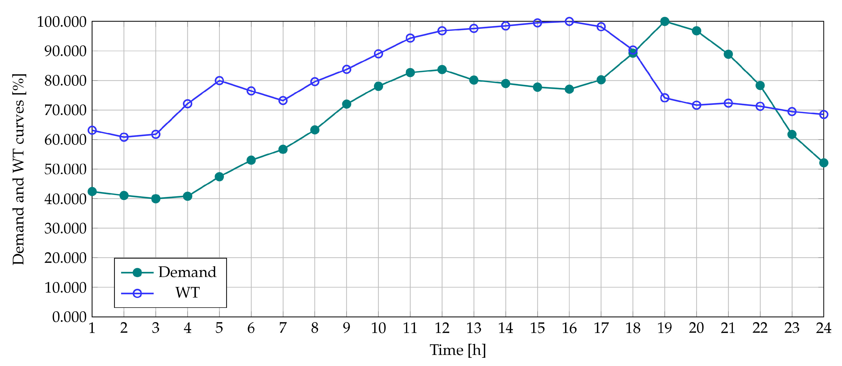
  • A methodology for optimal placement and sizing of wind power generators considering reactive power capability and wind speed curves is described. In addition, the methodology also takes into account demand curves over a 24-h period.
  • The proposed methodology is focused on minimizing power losses, which can be applied to radial and mesh networks.
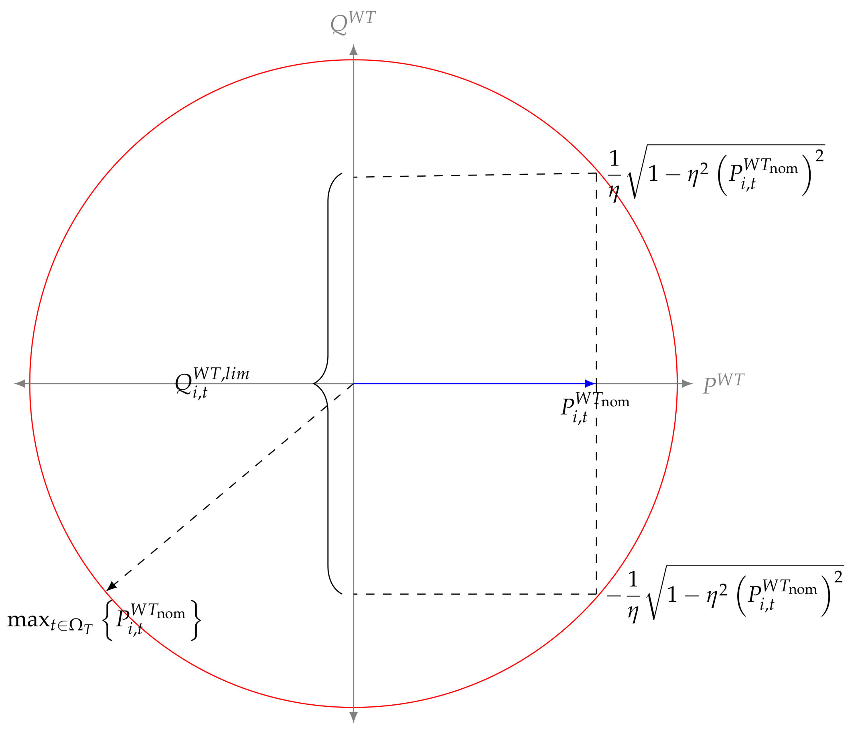
  • A chargeability factor η is proposed to represent the capacity to support the reactive power of a wind power system.
This study is organized as follows: Section 2 describes the mathematical modeling for the problem of the optimal location of wind power sources in AC distribution networks considering load variations and wind speed curves. Section 3 introduces the artificial neural network to forecast wind speed variations. Section 4 presents the main characteristics of the software implementation of the proposed mathematical model. In Section 5 the test system is presented, and Section 6 presents the numerical simulations. Lastly, the main concluding remarks derived from this research are shown in Section 7.

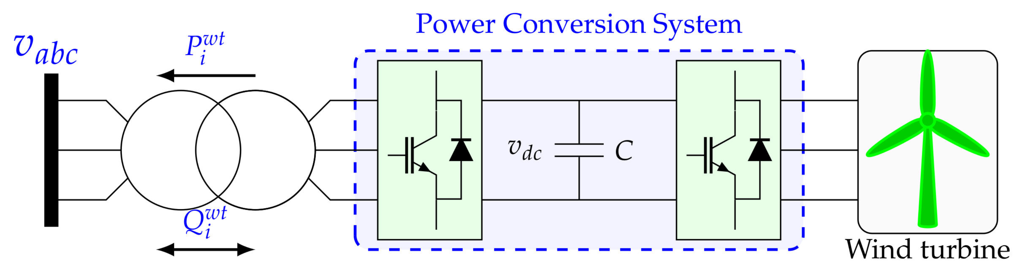
2. Mathematical Modeling

The problem of the optimal location of wind power sources in AC distribution networks considering load variations and wind speed curves is a nonlinear, non-differentiable, and non-convex optimization problem that combines continuous and discrete variables. In general terms, these characteristics generate an MINLP model, as reported in [5]. The main interest of this MINLP model is to minimize the total daily energy losses in all the branches of the AC grid. The complete mathematical model is presented below:
Objective function:
min   z = t Ω T i Ω N V i , t j Ω N V j , t Y i j cos θ i , t - θ j , t - ϕ i j Δ T ,
where z is the value of the objective function related to the minimization of the daily energy losses, V i , t ( V j , t ) is the voltage magnitude at node i (j) at the period of time t. Y i j is the magnitude of the admittance that relates nodes i and j. θ i , t ( θ j , t ) is the angle of the voltage at node i (j) at the period of time t; ϕ i j is the angle of the admittance that relates nodes i and j. Observe that Δ T is the period of time of the analysis (typically defined as 1 h for daily economic dispatch); and Ω N and Ω T are the sets that contain the nodes and the periods of time, respectively.
Set of constraints:
P i , t C G + y i W T P i , t W T nom - P i , t D = V i , t j Ω N V j , t Y i j cos θ i , t - θ j , t - ϕ i j ,   i Ω N , t Ω T
Q i , t C G + Q i , t W T - Q i , t D = V i , t j Ω N V j , t Y i j sin θ i , t - θ j , t - ϕ i j ,   i Ω N , t Ω T
V i min V i , t V i max ,   i Ω N , t Ω T
0 y i W T P i W T max x i W T ,      i Ω N
- y i W T η 1 - η 2 P i , t W T nom 2 Q i , t W T y i W T η 1 - η 2 P i , t W T nom 2 ,   i Ω N , t Ω T
i Ω N x i W T N G W T max ,
where P i , t C G is the active power generation at node i at the period of time t by the conventional generator; y i W T is the decision variable that defines the size of the wind turbine located at node i; P i , t W T nom is the nominal curve in per unit of the active power generated by the wind turbine connected at node i in the period of time t (this curve is obtained after applying the artificial neural network (ANN) forecasting methodology). P i , t D is the active power consumption at node i in the period of time t. Q i , t C G is the reactive power generation at node i at the period of time t by the conventional generator; Q i , t W T is the reactive power generated by the wind turbine connected at node i in the period of time t (this value depends of the active power transported by the paired wind turbine–power converters). Q i , t D is the reactive power consumption at node i in the period of time t. V i min and V i max are the minimum and maximum bounds for the voltage profile at node i. P i W T max is the maximum active power generation capability (size) of the wind turbine that can be connected at node i. x i W T is the binary variable related to the location of a wind turbine at node i, i.e., if x i W T = 1 the generator is located, and x i W T = 0 otherwise. The constant η corresponds to the chargeability factor of the paired wind turbine–power converter at the maximum active power point, i.e., 0 < η 1 . Here we assume that this chargeability factor equals 90 % . N G W T max is the maximum number of wind turbines available for location on the AC grid.
The mathematical model defined from (1) to (7) has the following interpretation: Equation (1) represents the objective function at it determines the total energy losses in an operation period of 24 h. In (2) and (3) are defined the active and reactive power balance equations; Expression (4) represents a box-type constraint that represents the minimum and maximum voltage regulation bounds in the AC grid. Equation (5) determines the size of the wind turbine that can be located at node i if the decision variable x i W T is activated. Equation (6) determines the maximum and minimum reactive power bounds of the wind turbine located at node i; note that this reactive power can be positive or negative, which implies that the wind turbine can work with lagging or leading power factor as variable energy compensator. In (7) the maximum number of wind turbines available for location in the AC grid is defined.
In Figure 1 the interconnection scheme of the wind turbine to the electrical AC network is presented. This connection is made via back-to-back voltage source converters. In this connection, via nonlinear control strategies such as passivity-based control [24,25], sliding mode control [26,27] or feedback linearization [28,29], among others, it is possible to control the active and reactive power flow exchanged between the AC grid and the wind turbine system independently.
Based on Figure 1, and considering that the power losses in the power conversion system and transformer are negligible, the reactive power inequality constraint reported in (6) is reached as follows: first, we assume that when the maximum active power is obtained from the wind turbine system the power conversion system works at 90%, we name this factor as η , which implies that under this condition, if a wind turbine is located at node i, the per unit representation is as follows:
max t Ω T P i , t W T nom = η S i W T nom .
Second, if we consider the reactive power variable Q i , t W T in per unit representation, then, the following result yields:
Q i , t W T = ± S i W T nom 2 - P i , t W T nom 2 .
Now, if we substitute (8) in (9), we obtain the result presented below:
Q i , t W T = ± 1 η max t Ω T P i , t W T nom 2 - η 2 P i , t W T nom 2 .
Since our interest is to support reactive power dynamically, we replace the equality sign in (10) by an inequality constraint as reported in (6). Observe that in per unit representation max t Ω T P i , t W T nom = 1 . Figure 2 illustrates the reactive power limits of wind energy for an active power delivered at the given time.
In the case of the real and imaginary power dispatches (control strategy), i.e., active and reactive power generation in WTs, it is important to mention that the control of these are made via nonlinear strategies applied to the power system conversion presented in Figure 1. This picture presents a type-D (or Type-4) WT connection, where the first voltage source converter controls the active power providing by the wind generator and supports all its reactive power requirements. While the second voltage source converter adjusts this active power to be transferred to the electrical grid with an adequate frequency at the same time that interchanges reactive power with this [30]. In addition, the voltage source converter also enables reactive power to be delivered or absorbed. In this part, we are interested in presenting the tertiary control stage in power system operation, i.e., the optimization stage in hierarchical control structures. The tertiary control stage is also called optimal power flow and it can be implemented as centralized or distributed [31]. This works if links are sent to each active device (e.g., power electronic converters) to provide references to primary and secondary controls [32].

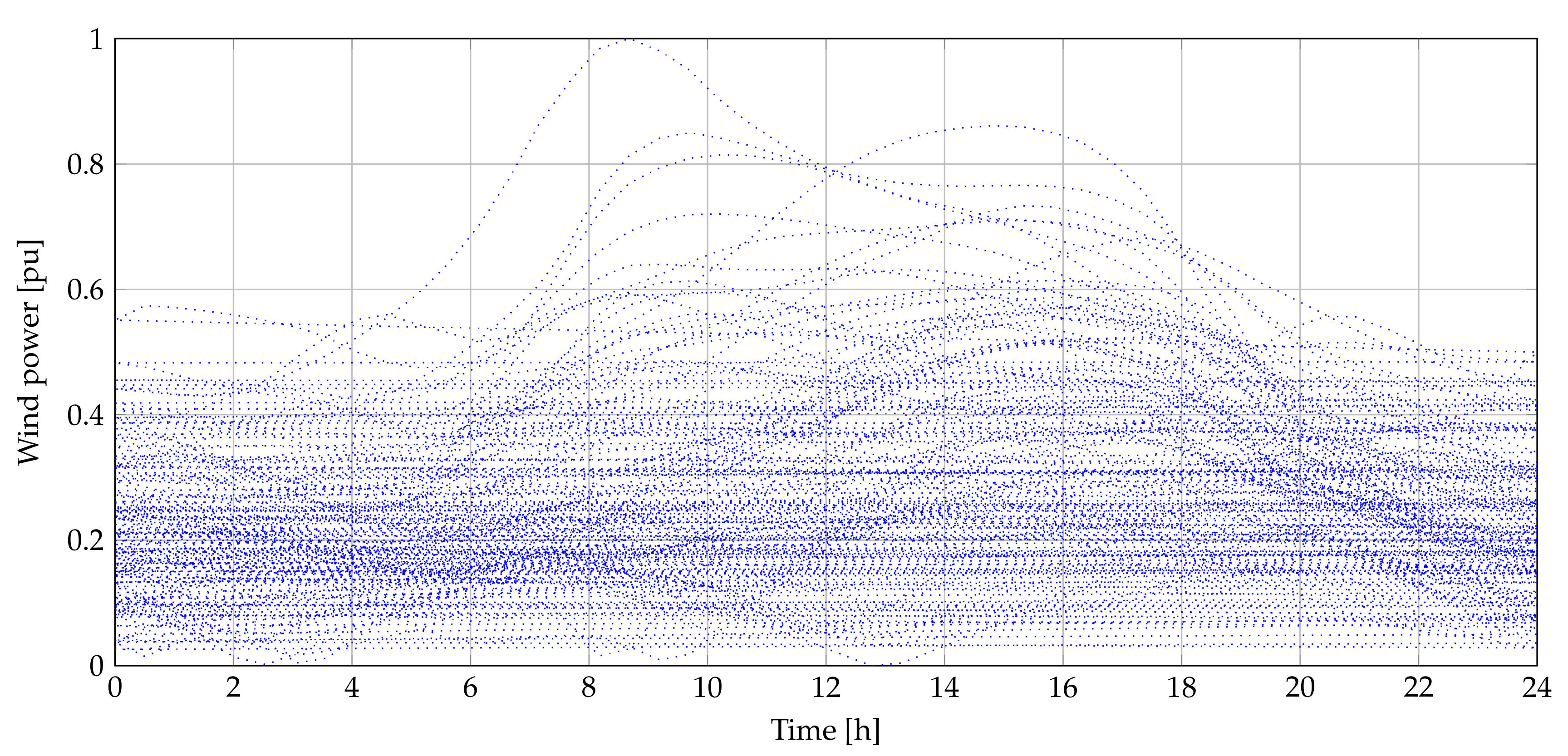
3. Wind Power Forecasting

The integration of renewable energy sources is a great challenge, framed in the intermittence of their primary resources. Therefore, it is essential to consider these intermittences in the planning, and their potential for power generation. Additionally, improper placement and sizing of the wind powers may cause troubles, such as transmission line overload, voltage profiles, and increases in power losses [33]. Hence, the placement and sizing of these generators should take into account the high variability of the wind speed with the purpose of minimizing the forecasting errors and, therefore, avoiding the issues mentioned above.
Here we adopt the methodology proposed in [23], which is based on ANN. The ANN needs as input information the temperature, humidity, pressure, and time to properly estimate the wind speed. The historical wind speed data are depicted in Figure 3, which are taken from [33] and [34].
Note in Figure 3 that the illustrated wind speed comprises multiple days over the course of the 24-h period, which provides the ANN with sufficient information to make an adequate prediction. It is also important to mention although the plots are not shown for the temperature, humidity, pressure, and time, this information is also implemented for the ANN. These data are found in the Caribbean region of Colombia, and the availability of wind speed energy is measured over a year.

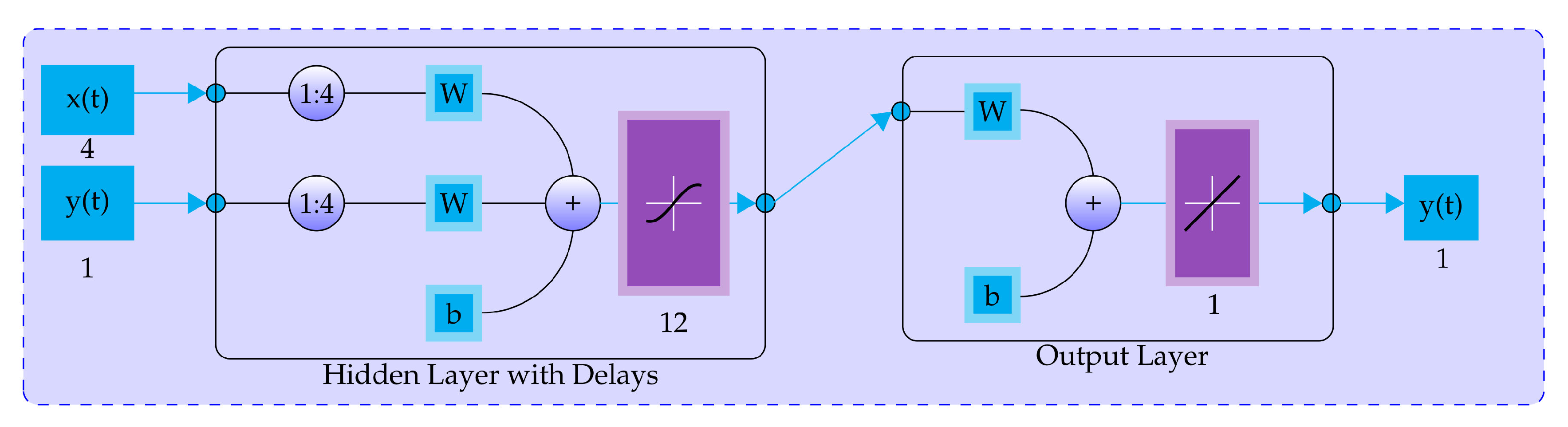
Artificial Neural Network

The ANN has implemented several topics, such as pattern classification, clustering, optimization, function approximation, and prediction [35]. The ANN is a mathematical tool that can store and remind the characteristics of a system and, therefore, obtain learning for the purpose of predicting future events or stochastic variables. The ANN has some advantages such as fast time in processing information and small data size, no complexity in pattern recognition tasks, and reprogramming is not required [36].
The training process of an ANN requires input and output data of the system to obtain a nonlinear mapping. The ANN is implemented when it does not have a system model in which the input and output data are related. The nonlinear learning rule is reached, as follows:
y ( t ) = f y ( t - 1 ) , . . . , y ( t - n y ) , x ( t - 1 ) , . . . , x ( t - n x )
where x R n and y R are input and output data. n y and n x are the last values of the prediction and the input data, respectively. Observe that y also depends on the last n y values of the variable under prediction.
The ntstool of MATLAB software was used in the training process of the ANN to predict the wind speed. The ANN configuration is composed of four inputs (temperature, humidity, pressure, and time), four delays, and 12 hidden neurons. We set up the ANN in the training, adjustment, and validation processes with a 70%, 15%, and 15% of the data, respectively. In Figure 4 the ANN scheme with the wind speed predictions implemented in MATLAB is shown.

4. Solution Methodology

To solve the MINLP model that represents the optimal placement and sizing of wind turbines in AC distribution networks considering wind and demand curves, in this research the general algebraic modeling system is employed, widely known in specialized literature as GAMS. This optimization package has been successfully used for solving nonlinear large-scale optimization problems, such as optimal location and sizing of distributed generators in AC and DC distribution networks [5,37]; optimal operation of battery energy storage systems [23,38]; multi-objective optimization of the stack of a thermoacoustic engine [39] and optimization of pump and valve schedules in complex, large-scale water distribution systems [40], and so on. The main characteristics of GAMS implementation are listed below [23].
Representation of the mathematical models by sets, which generates a compact formulation.
The mathematical structure of the model, i.e., (1)–(7), is preserved via symbolic representation by using a plain text.
This optimization software allows solving multiple optimization problems, such as linear programming, discrete models, and general non-convex formulations.
Availability of a free version for demonstration, useful to introduce undergraduate students with mathematical optimization.
Non-advanced programming skills are required for using GAMS, since it has an intuitive manner to implement a mathematical model using a basic plain text interface.
The basic elements for implementing a mathematical model in the GAMS interface are presented in Algorithm 1.
Algorithm 1: Main features for implementing a mathematical optimization model in GAMS
Data: Define the nature of the optimization problem and select the test system.
Sets Definition of sets, parameters (constant vectors), scalars (constant number), and tables (constant matrices).
Variables: Determine the type of variables, e.g., integer, continuous or binary.
Equations: Write the optimization problem, i.e., the set of Equations (1)–(7).
Solution: Select a MINLP solver to reach the solution via minimization of the objective function.
Visualization: Extract the variables of interest, i.e., location of the generators and their sizes, the value of the objective function, etc.
Result: Optimal location and sizing of wind turbines in AC distribution networks under daily operative scenarios.
General characteristics about GAMS implementations, such as reserve words and specialized functions can be consulted in [41].

5. Test Systems

To validate the proposed mathematical model for optimal location and placement of renewable energy sources such as wind power considering reactive power capabilities in AC distribution networks, we consider two test systems with a radial structure composed of 27 and 69 nodes, respectively. These systems are presented below.

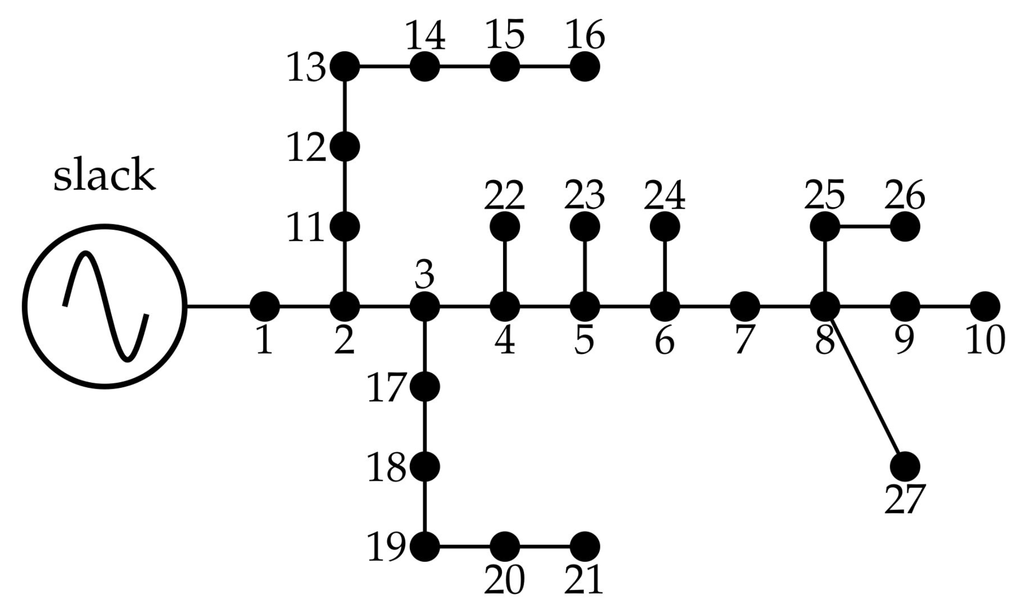
5.1. 27-Node Test System

The 27-node test system is a radial test system with similar characteristics of the Colombian distribution networks located in the Caribbean region [37]. The branch information and nodal demands at the peak hour are reported in Table 1, and the electrical configuration of this test feeder is depicted in Figure 5. For this test system, we employ 13 . 8 kV and 1000 kW as voltage and power bases, respectively. To evaluate the daily operation of this system, including PV systems, we employ the demand variation and the wind generation capacity reported in Figure 6. Note that in this test feeder, the maximum size of each wind turbine is left free to verify the effect of the renewable injection to reduce the daily energy losses.

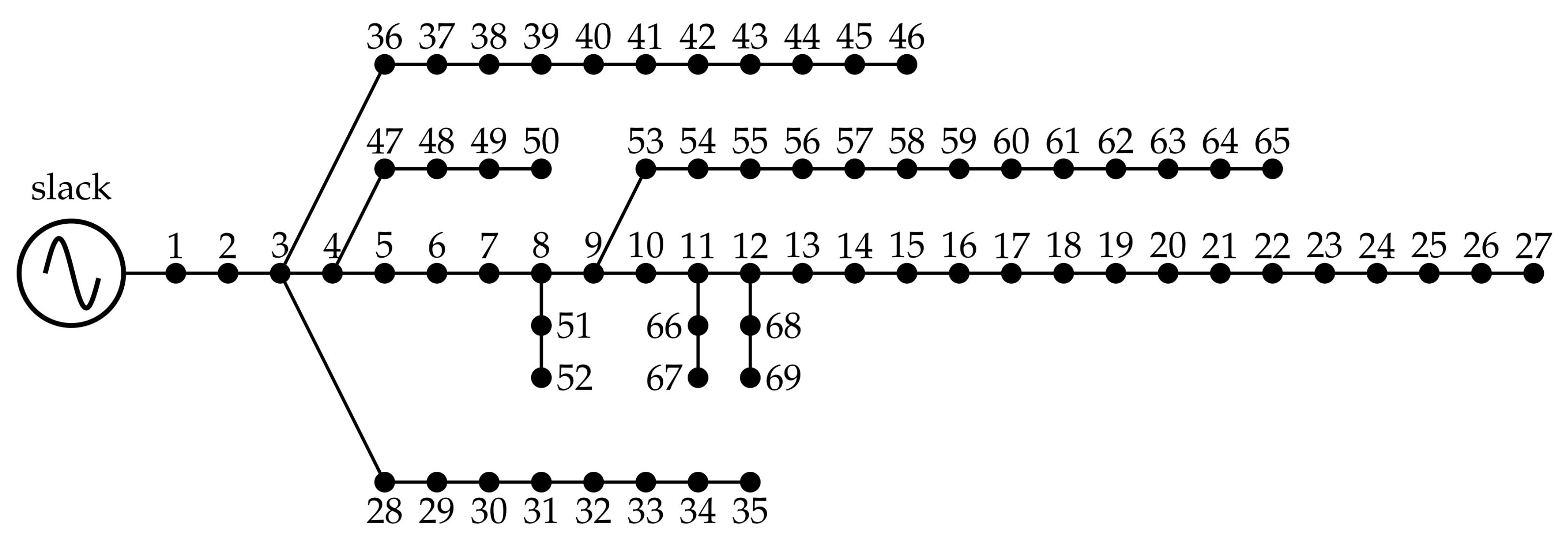
5.2. 69-Node Test Feeder

This test feeder illustrated in Figure 7 is widely known in specialized literature as the Baran and Wu test system with 69 nodes and 68 branches with 12 . 66 kV of operating voltage [21]. This test feeder has 3890 . 7 kW and 2693 . 6 kVAr of total active and reactive power demand. The initial active energy losses of this system equals 3525 . 7520 kWh/day. For this test system, we also considered the possibility of installing 3 wind turbines, limited from 0 kW to 2000 kW each. In addition, we also considered 12 . 66 kV and 1000 kW as voltage and power base values, respectively.
The information of the branches and the load consumption of the 69-node test feeder is presented in Table 2. Additionally, the demand and wind turbine curves are the same presented in Figure 6.

6. Computational Validation

The solution of the general MINLP model defined from (1) to (7) for the optimal placement and sizing of wind turbines considering reactive power capabilities is made using the GAMS optimization package with the CONOPT solver in a desktop computer with an INTEL(R) Core(TM) i5-3550 3.5 GHz processor and 8 GB of RAM running a 64-bit version of Windows 7 Professional [37].
In order to verify the effectiveness of using wind turbines considering the reactive power capability in the converters, we solve the problem from zero to three possible distributed generators considering unity power factor and reactive power injections; these cases allow to detect the effect of reactive power compensation in the daily operative behavior of the AC distribution systems in regards to the energy losses minimization [5].

6.1. 27-Node Test Feeder

For this test system we evaluate the the operation of the paired wind turbine power electronic converter with unity and variable power factor. In Table 3 the solution achieved by GAMS considering unity power factor is reported and in Table 4 the solution with variable reactive power compensation is presented. Note that in these simulation results, the chargeability factor is selected as η = 0 . 9 p.u. In this test system the daily energy losses is 1652 . 0190 kWh/day.
Results in Table 3 and Table 4 show the positive effect of including renewable generation in the daily operation of AC distribution networks. It is important to mention that depending on the operative consign of the wind turbine, i.e., unity power factor or variable power factor, the location and size of the generators are susceptible to change; for example in the case of three WTs when power factor is unitary, the location of the generators is at nodes 8, 15, and 20 with a total active power generation at the peak hour about 2350 . 4561 kW; while in the case of the variable power factor the location of the generators is at nodes 9, 13 and 19, with a total active power generation at the peak hour about 2343 . 2501 kW. Note that nodes suffer slight variations in their locations for both scenarios, nevertheless, with a little reduction of the total power capability ( 7 . 2060 kW) the variable power factor approach allows a reduction in about 345 . 2682 kWh/day passing from 628 . 4598 kWh/day to 283 . 1916 kWh/day when unitary power factor changes from being unitary to variable. The previous results confirm the conclusions reached by authors of [6], where both cases were analyzed for AC distributed networks considering only the peak hour in their analysis.
Results in Figure 8 confirm the positive effect of using variable power factor in wind turbine applications via power conversion system to dynamically support active and reactive power to the AC grid. In this sense, for one WT the reduction in the daily energy losses is about 21 . 62 % , for two WTs is about 14 . 59 % , and for three wind turbines is about 20 . 90 % when compared unitary and variable power factor approaches.
An important fact in the results presented in Figure 8 is that there is no linear relation between the number of renewable sources placed in the distribution system and the energy losses reduction, since the effect of an additional renewable source is less in comparison with the previous case, as concluded in [37] for photovoltaic plants. This behavior is expected, since the objective function (1) is nonlinear and non-convex, which implies that linear tendencies cannot be extrapolated from it.
It is worthy to mention that for this test feeder when unitary power factor is considered the GAMS package takes about 25 s to solve the problem, while in the variable power factor case this time is increased to 45 s. This increment is caused by the fact that in the variable power factor scenario appears the amount of reactive power as a variable, which introduces complexity to the optimization model and the solution space increases substantially with a rate of about 24 additional variables per WT.

6.2. 69-Node Test Feeder

Table 5 and Table 6 present the optimal location and sizing of wind turbines in the 69-node test feeder considering unity and variable power factor, respectively.
In the case of the unitary power factor approach reported in Table 5 we can observe node 60 with a strong effect in the energy losses reduction, since in all the three cases, it appears with important power injections. Here it is important to mention that for one WT, the daily energy losses are about 1179 . 3480 kWh/day; while for three WT units this number is reduced to 949 . 2134 kWh/day. This implies that the nonlinear relation between number of renewable sources and energy losses is strongly demonstrated in the 69-node test feeder, since the difference in both cases is only 230 . 1346 kWh/day passing from 1639 . 2766 kW to 1993 . 7893 kW in the peak hour regarding the amount of power installed, i.e., 354 . 5127 kW of additional power.
When variable power factor is analyzed the effect of reactive power injection is evident (see Table 6), since the daily energy losses present strong reduction for all the combinations of wind turbines. For example, if we observe the case of two WTs, then, the daily energy losses pass from 1048 . 7920 kWh/day to 268 . 0452 kWh/day by injecting at the peak hour a total of 2034 . 4016 kW; which is similar to the 2004 . 4763 kW in the unitary power factor scenario. Figure 9 confirms that the variable power factor approach increases by about 30 % the daily losses reduction when compared to unitary power factor approach. This result indicates that distributed generators with dynamic reactive power compensation can be a powerful alternative to improve the electrical performance of the AC distribution networks, only by using adequate control schemes in the power conversion system presented in Figure 1.
Similarly, as shown by the 27-node test system, in the 69-node case the number of generators and their impact in the total energy losses reduction is strongly nonlinear, since for two and three WTs we observe a clear saturation in the objective function performance, with a small increment of about 5%. This implies that for utilities it is important to consider these nonlinear phenomena in their grids, since large penetrations of renewable energy can affect negatively their electric power system performances.
The processing times required in the case of the 69-node test feeder when the unity power factor was used was about 120 s, while in the case of the variable power factor, it increases to 450 s. This increment has the same explanation presented for the 27-node test feeder, and it is related to the increment in the number of variables in the optimization problem.

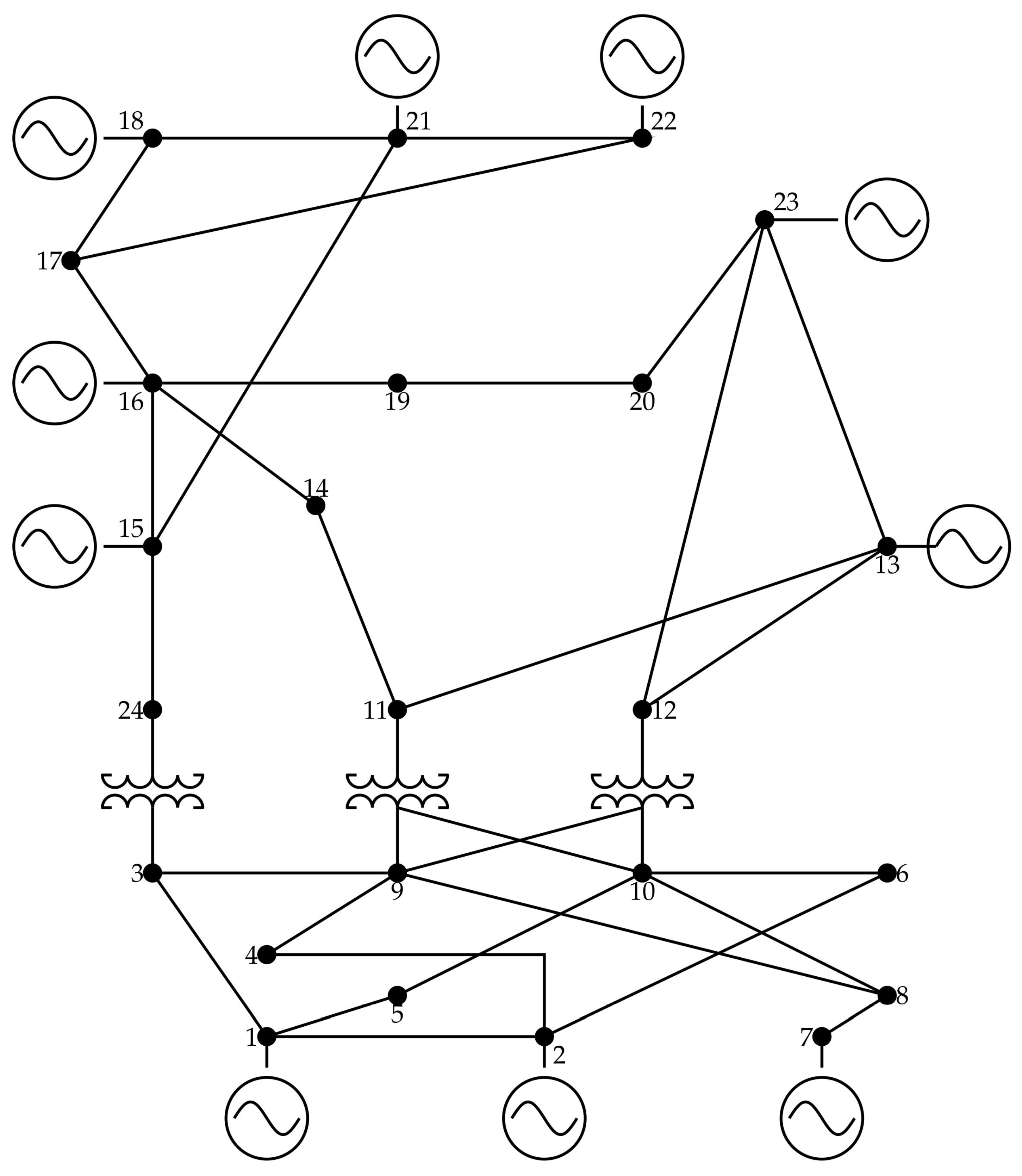
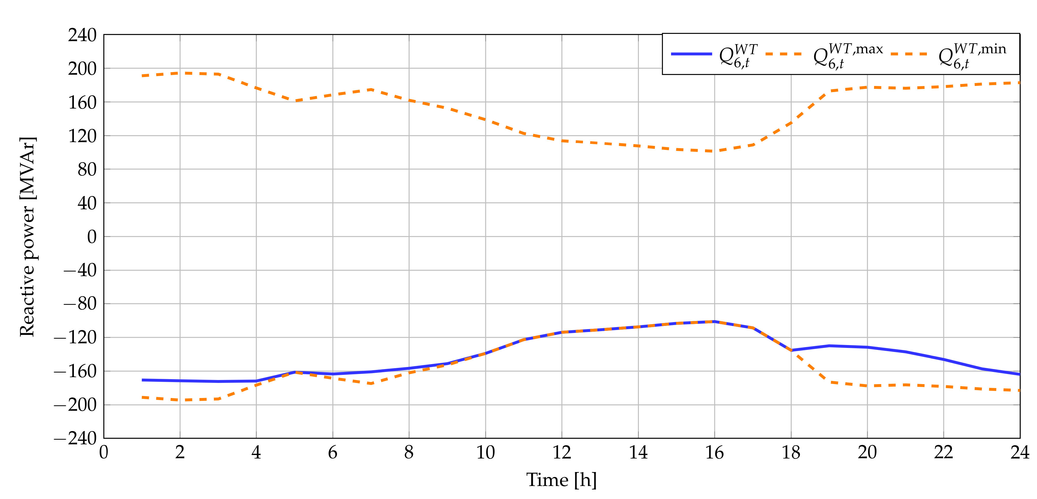
6.3. Large-Scale Power System Evaluation

To evaluate the applicability of the proposed mathematical model for optimal location and sizing of wind turbines in electrical networks with reactive power capabilities via power electronic converters, we implement a large-scale power system composed of 24 nodes with 38 interconnections via transmission lines and transformers [42,43]. This system has a total of active and reactive power demands of about 2850 MW and 580 MVAr, respectively. In addition, these power demands are fed by 10 conventional generators and 1 reactive power compensator. The electrical configuration of this test feeder is presented in Figure 10 and the parameters are reported in Table 7, Table 8 and Table 9, respectively (the voltage and power bases for this test feeder are 100 MW and 220 kV). For this test system, we assume that the slack node corresponds to the generator located at node 13, which is set with voltage output of 1 . 050 p.u. It is important to mention that the rest of the generators are free for generating the required power to minimize the total daily energy losses, and the voltage regulation bounds for this power system are 0 . 900 p.u. and 1 . 100 p.u., respectively.
To simulate the 24-node test feeder, we consider the case that reactive power is available to be injected into the power system since results for 27- and 69-node test feeders have demonstrated that variable power is more efficient regarding energy losses reduction than unity power factor. In Table 10 the optimal solutions reached by the GAMS package is reported on the high-voltage meshed power system depicted in Figure 10.
From the results in Table 10, we can observe that:
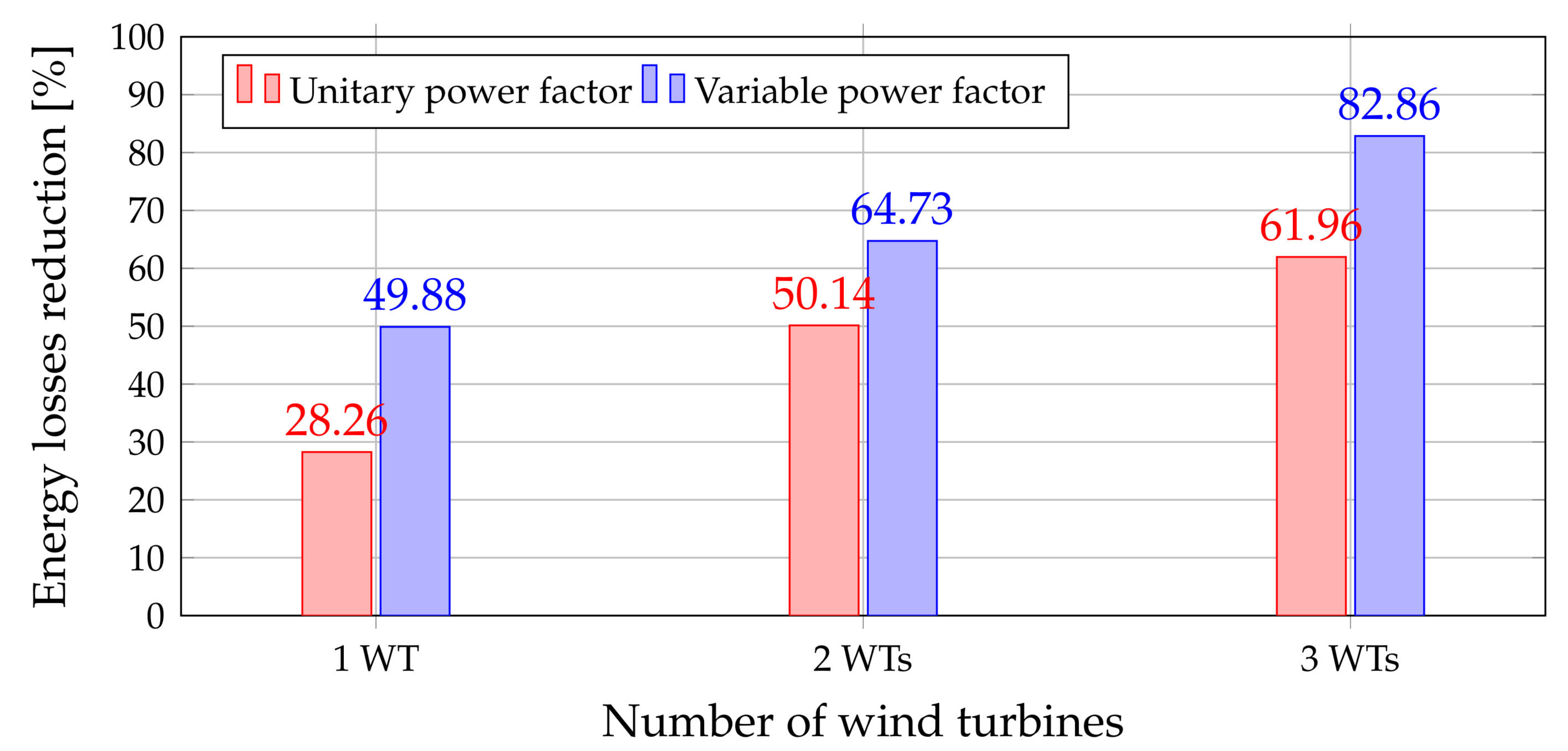
  • To reach a total daily energy losses reduction of about 45 . 0384 % it is required to install a WT at node 6 with a nominal rate of 208 . 9887 MW; and to increase the daily energy reduction by 13 . 7075 %, 576 . 2719 MW is required to be installed, which implies more than 100 % of additional power injection. This result implies that energy losses formulated in (1) have a strong nonlinear relation between the amount of power injection by renewable energy resources and their location in regards with the objective function minimization. Note that this behavior was also observed in both radial test feeders previously reported.
  • The proposed mathematical model is suitable to be applied for both radial medium voltage and high-voltage meshed networks, which confirms that it is general and scalable for multiple grid topologies.
On the other hand, Figure 11 presents the behavior of the reactive power for the case of the installation of one wind turbine at node 6.
Observe that positive and negative reactive power bounds depicted in Figure 11 correspond to the graphical behavior of constraint (6) when y 6 W T is 208.9887 MW. It is important to highlight that these bounds are variable as a function of the active power generation since the power electronic converter that interfaces this WT has limited apparent power capabilities and function of the chargeability factor η , as demonstrated in Section 2. Finally, it is worth mentioning that in the case of the one wind turbine, the power electronic converter works in the second quadrant, because it provides active power at the same time that absorbs reactive power. This implies that this converter is absorbing the excessive reactive energy supplied by all the conventional power sources.

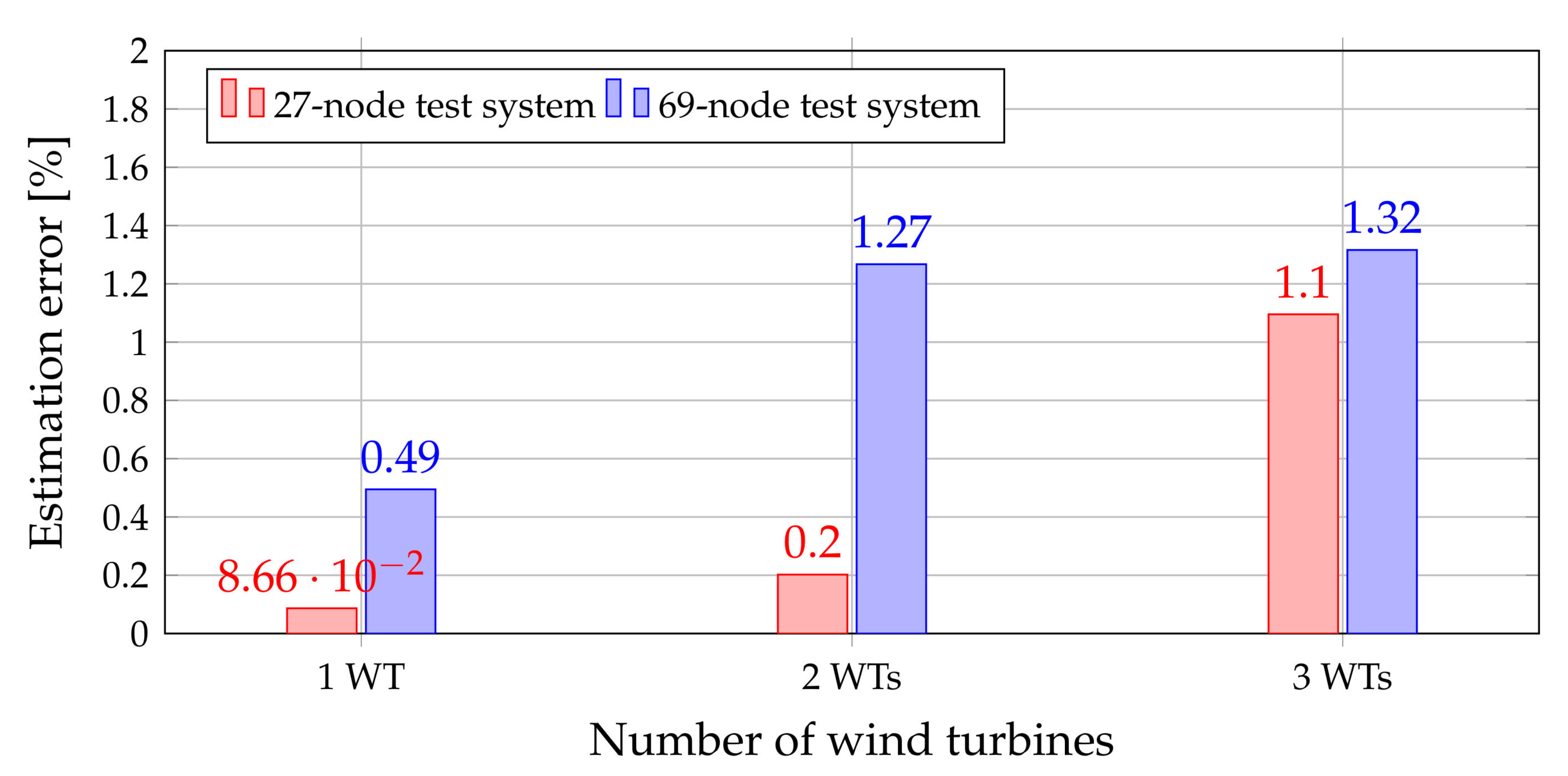
6.4. Assessment of ANN Performance

To demonstrate the efficiency of the ANN approach for predicting the renewable energy availability in wind turbines, we fix the locations reported in Table 4 for the 27-node test feeder and Table 6 for the 69-node test feeder for the WTS to evaluate the objective function when using the real wind energy curve (the real wind power curve can be consulted in [23]). In Figure 12 the absolute error regarding the objective function between the real and estimated curves for both test systems is presented. Note that the error reported in this picture is calculated, as follows:
ϵ = v r - v e v r ,
where ϵ is the estimation error, v r is the real value of the objective function and v e the estimation reached with the ANN prediction.
Figure 12 reports the estimation errors reached when the ANN prediction is compared with the real generation curve. This picture allows to conclude that the maximum error for both test feeder does not overpass 1.35% for different possibilities of wind turbine locations. This result confirms that the ANN is a powerful tool for renewable generation prediction, as previously published in [5,23] for wind and photovoltaic applications.

7. Conclusions and Future Works

The variable energy compensation problem in AC distribution networks has been analyzed in this paper via optimal placement and sizing of wind turbines, considering daily wind and demand curves. The main contribution of this study is the nonlinear formulation related to the paired wind turbine and power conversion system via chargeability factor η at the peak hour. This factor represents the percentage of usage of the power conversion system in the nominal wind speed conditions, and it allows supporting reactive power dynamically during all periods of the day as a function of the distribution system requirements.
The effect of the variable power factor in comparison to the unitary scenario was evident for both test feeders since the reduction of the energy losses was at least 20 % superior by using practically the same installed capability regarding active power injection at the peak hour. These results confirm that power conversions systems presented in the integration of renewable can be used to replace classical approaches, such as capacitor banks with fixed of variable steps. Power conversion systems can be operated with lagging or leading power factors, which is a definite advantage in variable demand scenarios.
Artificial neural networks employed for renewable generation forecasting evidenced estimation errors lower than 1 . 35 % when real and predicted curves are compared in terms of the objective function estimation, which allows to demonstrate the efficiency and robustness of this tool for economic and optimal power dispatch problems in the presence of renewable uncertainties.
As future work, it will be possible to solve the proposed optimization problem via metaheuristic techniques by using a master-salve structure with genetic algorithms and vortex optimizers. Additionally, it will also be possible to include the chargeability factor η as an optimization variable. This will allow to identify the optimal size of the power conversion system. An additional future work might be related to the inclusion of contingency analysis in meshed power systems in order to identify the best location and size of the renewable source to make the entire system more reliable and secure under fault conditions.

Author Contributions

Conceptualization and writing—Review and editing, W.G.-G., O.D.M., L.F.G.-N., A.-J.P.-M. and Q.H.-E. All authors have read and agreed to the published version of the manuscript.

Funding

This work was partially supported by the National Scholarship Program Doctorates of the Administrative Department of Science, Technology, and Innovation of Colombia (COLCIENCIAS) by calling contest 727-2015.

Conflicts of Interest

The authors declare no conflicts of interest.

References

  1. Mazhari, S.M.; Monsef, H.; Romero, R. A multi-objective distribution system expansion planning incorporating customer choices on reliability. IEEE Trans. Power Syst. 2015, 31, 1330–1340. [Google Scholar] [CrossRef]
  2. Essallah, S.; Khedher, A.; Bouallegue, A. Integration of distributed generation in electrical grid: Optimal placement and sizing under different load conditions. Comput. Electr. Eng. 2019, 79, 106461. [Google Scholar] [CrossRef]
  3. Mohseni-Bonab, S.M.; Rabiee, A. Optimal reactive power dispatch: A review, and a new stochastic voltage stability constrained multi-objective model at the presence of uncertain wind power generation. IET Gener. Transm. Distrib. 2017, 11, 815–829. [Google Scholar] [CrossRef]
  4. Strunz, K.; Abbasi, E.; Huu, D.N. DC microgrid for wind and solar power integration. IEEE Trans. Emerg. Sel. Top. Power Electron. 2013, 2, 115–126. [Google Scholar] [CrossRef]
  5. Montoya, O.D.; Grisales-Noreña, L.F.; Gil-González, W.; Alcalá, G.; Hernandez-Escobedo, Q. Optimal Location and Sizing of PV Sources in DC Networks for Minimizing Greenhouse Emissions in Diesel Generators. Symmetry 2020, 12, 322. [Google Scholar] [CrossRef] [Green Version]
  6. Kaur, S.; Kumbhar, G.; Sharma, J. A MINLP technique for optimal placement of multiple DG units in distribution systems. Int. J. Electr. Power Energy Syst. 2014, 63, 609–617. [Google Scholar] [CrossRef]
  7. Ghosh, S.; Ghoshal, S.P.; Ghosh, S. Optimal sizing and placement of distributed generation in a network system. Int. J. Electr. Power Energy Syst. 2010, 32, 849–856. [Google Scholar] [CrossRef]
  8. Manikanta, G.; Mani, A.; Singh, H.; Chaturvedi, D. Placing distributed generators in distribution system using adaptive quantum inspired evolutionary algorithm. In Proceedings of the Second International Conference on Research in Computational Intelligence and Communication Networks (ICRCICN), Kolkata, India, 23–25 September 2016; pp. 157–162. [Google Scholar]
  9. Babu, P.V.; Singh, S. Optimal Placement of DG in Distribution network for Power loss minimization using NLP & PLS Technique. Energy Procedia 2016, 90, 441–454. [Google Scholar]
  10. Meena, N.K.; Swarnkar, A.; Gupta, N.; Niazi, K. Wind Power Generation Planning by Utilizing the Reactive Power Capabilities of Generators. In Proceedings of the Asian Conference on Energy, Power and Transportation Electrification (ACEPT), Singapore, 24–26 October 2017; pp. 1–6. [Google Scholar]
  11. Prabha, D.R.; Jayabarathi, T. Optimal placement and sizing of multiple distributed generating units in distribution networks by invasive weed optimization algorithm. Ain Shams Eng. J. 2016, 7, 683–694. [Google Scholar] [CrossRef] [Green Version]
  12. Jamil, M.; Anees, A.S. Optimal sizing and location of SPV (solar photovoltaic) based MLDG (multiple location distributed generator) in distribution system for loss reduction, voltage profile improvement with economical benefits. Energy 2016, 103, 231–239. [Google Scholar] [CrossRef]
  13. Das, B.; Mukherjee, V.; Das, D. DG placement in radial distribution network by symbiotic organisms search algorithm for real power loss minimization. Appl. Soft Comput. 2016, 49, 920–936. [Google Scholar] [CrossRef]
  14. Parizad, A.; Khazali, A.H.; Kalantar, M. Sitting and sizing of distributed generation through Harmony Search Algorithm for improve voltage profile and reducuction of THD and losses. In Proceedings of the CCECE 2010, Calgary, AB, Canada, 2–5 May 2010; pp. 1–7. [Google Scholar]
  15. Abu-Mouti, F.S.; El-Hawary, M. Optimal distributed generation allocation and sizing in distribution systems via artificial bee colony algorithm. IEEE Trans. Power Deliv. 2011, 26, 2090–2101. [Google Scholar] [CrossRef]
  16. García, J.A.M.; Mena, A.J.G. Optimal distributed generation location and size using a modified teaching–learning based optimization algorithm. Int. J. Electr. Power Energy Syst. 2013, 50, 65–75. [Google Scholar] [CrossRef]
  17. Cheng, S.; Chen, M.Y.; Fleming, P.J. Improved multi-objective particle swarm optimization with preference strategy for optimal DG integration into the distribution system. Neurocomputing 2015, 148, 23–29. [Google Scholar] [CrossRef]
  18. Tolabi, H.B.; Ali, M.H.; Rizwan, M. Simultaneous reconfiguration, optimal placement of DSTATCOM, and photovoltaic array in a distribution system based on fuzzy-ACO approach. IEEE Trans. Sustain. Energy 2014, 6, 210–218. [Google Scholar] [CrossRef]
  19. Muthukumar, K.; Jayalalitha, S. Optimal placement and sizing of distributed generators and shunt capacitors for power loss minimization in radial distribution networks using hybrid heuristic search optimization technique. Int. J. Electr. Power Energy Syst. 2016, 78, 299–319. [Google Scholar] [CrossRef]
  20. Kefayat, M.; Ara, A.L.; Niaki, S.N. A hybrid of ant colony optimization and artificial bee colony algorithm for probabilistic optimal placement and sizing of distributed energy resources. Energy Convers. Manag. 2015, 92, 149–161. [Google Scholar] [CrossRef]
  21. Grisales-Noreña, L.F.; Gonzalez Montoya, D.; Ramos-Paja, C.A. Optimal sizing and location of distributed generators based on PBIL and PSO techniques. Energies 2018, 11, 1018. [Google Scholar] [CrossRef] [Green Version]
  22. Martinez-Rojas, M.; Sumper, A.; Gomis-Bellmunt, O.; Sudrià-Andreu, A. Reactive power dispatch in wind farms using particle swarm optimization technique and feasible solutions search. Appl. Energy 2011, 88, 4678–4686. [Google Scholar] [CrossRef]
  23. Montoya, O.D.; Gil-González, W.; Grisales-Noreña, L.; Orozco-Henao, C.; Serra, F. Economic Dispatch of BESS and Renewable Generators in DC Microgrids Using Voltage-Dependent Load Models. Energies 2019, 12, 4494. [Google Scholar] [CrossRef] [Green Version]
  24. Cisneros, R.; Mancilla-David, F.; Ortega, R. Passivity-Based Control of a Grid-Connected Small-Scale Windmill With Limited Control Authority. IEEE J. Emerg. Sel. Top. Power Electron. 2013, 1, 247–259. [Google Scholar] [CrossRef]
  25. Namazi, M.M.; Nejad, S.M.S.; Tabesh, A.; Rashidi, A.; Liserre, M. Passivity-Based Control of Switched Reluctance-Based Wind System Supplying Constant Power Load. IEEE Trans. Ind. Electron. 2018, 65, 9550–9560. [Google Scholar] [CrossRef] [Green Version]
  26. Barambones, O. Sliding Mode Control Strategy for Wind Turbine Power Maximization. Energies 2012, 5, 2310–2330. [Google Scholar] [CrossRef]
  27. Lee, S.W.; Chun, K.H. Adaptive Sliding Mode Control for PMSG Wind Turbine Systems. Energies 2019, 12, 595. [Google Scholar] [CrossRef] [Green Version]
  28. Alrifai, M.; Zribi, M.; Rayan, M. Feedback Linearization Controller for a Wind Energy Power System. Energies 2016, 9, 771. [Google Scholar] [CrossRef] [Green Version]
  29. Li, P.; Wang, J.; Xiong, L.; Wu, F. Nonlinear Controllers Based on Exact Feedback Linearization for Series-Compensated DFIG-Based Wind Parks to Mitigate Sub-Synchronous Control Interaction. Energies 2017, 10, 1182. [Google Scholar] [CrossRef] [Green Version]
  30. Salgado-Herrera, N.M.; Medina-Ríos, A.; Tapia-Sánchez, R.; Anaya-Lara, O. Reactive power compensation through active back to back converter in type-4 wind turbine. In Proceedings of the IEEE International Autumn Meeting on Power, Electronics and Computing (ROPEC), Ixtapa, Mexico, 9–11 November 2016; pp. 1–6. [Google Scholar]
  31. Murillo-Yarce, D.; Garcés-Ruiz, A.; Escobar-Mejía, A. Passivity-Based Control for DC-Microgrids with Constant Power Terminals in Island Mode Operation. Revista Facultad de Ingeniería Universidad de Antioquia 2018, 86, 32–39. [Google Scholar] [CrossRef]
  32. Choi, Y.H.; Cho, Y.S. Multiple-Point Voltage Control to Minimize Interaction Effects in Power Systems. Energies 2019, 12, 274. [Google Scholar] [CrossRef] [Green Version]
  33. Gil-González, W.; Montoya, O.D.; Holguín, E.; Garces, A.; Grisales-Noreña, L.F. Economic dispatch of energy storage systems in dc microgrids employing a semidefinite programming model. J. Energy Storage 2019, 21, 1–8. [Google Scholar] [CrossRef]
  34. Data, S.S.R. Time Series of Solar Radiation Data. Available online: http://www.soda-pro.com/ (accessed on 5 July 2019).
  35. Koo, J.; Han, G.D.; Choi, H.J.; Shim, J.H. Wind-speed prediction and analysis based on geological and distance variables using an artificial neural network: A case study in South Korea. Energy 2015, 93, 1296–1302. [Google Scholar] [CrossRef]
  36. Demuth, H.B.; Beale, M.H.; De Jess, O.; Hagan, M.T. Neural Network Design, 2nd ed.; Martin Hagan: Stillwater, OK, USA, 2014. [Google Scholar]
  37. Montoya, O.D.; Gil-González, W.; Grisales-Noreña, L. An exact MINLP model for optimal location and sizing of DGs in distribution networks: A general algebraic modeling system approach. Ain Shams Eng. J. 2019. [Google Scholar] [CrossRef]
  38. Montoya, O.D.; Grajales, A.; Garces, A.; Castro, C.A. Distribution Systems Operation Considering Energy Storage Devices and Distributed Generation. IEEE Lat. Am. Trans. 2017, 15, 890–900. [Google Scholar] [CrossRef]
  39. Tartibu, L.; Sun, B.; Kaunda, M. Multi-objective optimization of the stack of a thermoacoustic engine using GAMS. Appl. Soft Comput. 2015, 28, 30–43. [Google Scholar] [CrossRef]
  40. Skworcow, P.; Paluszczyszyn, D.; Ulanicki, B.; Rudek, R.; Belrain, T. Optimisation of Pump and Valve Schedules in Complex Large-scale Water Distribution Systems Using GAMS Modelling Language. Procedia Eng. 2014, 70, 1566–1574. [Google Scholar] [CrossRef] [Green Version]
  41. Giraldo, O.D.M. Solving a Classical Optimization Problem Using GAMS Optimizer Package: Economic Dispatch Problem Implementation. Ing. Y Cienc. 2017, 13, 39–63. [Google Scholar] [CrossRef] [Green Version]
  42. Soroudi, A. Power System Optimization Modeling in GAMS; Springer International Publishing: Cham, Switzerland, 2017. [Google Scholar]
  43. Martínez-Lacañina, P.J.; Marcolini, A.M.; Martínez-Ramos, J.L. DCOPF contingency analysis including phase shifting transformers. In Proceedings of the Power Systems Computation Conference, Wroclaw, Poland, 18–22 August 2014; pp. 1–7. [Google Scholar]
Figure 1. Electrical interconnection of a wind turbine to AC three-phase distribution network via voltage source converters using back-to-back configuration for type-D connections [30].
Sustainability 12 02983 g001
Figure 2. Example of reactive power limits for an active power delivered.
Sustainability 12 02983 g002
Figure 3. Historical wind speed data used for the artificial neural network (ANN) training process (adapted from [23,33]).
Sustainability 12 02983 g003
Figure 4. ANN scheme for wind speed prediction [23].
Sustainability 12 02983 g004
Figure 5. Electrical configuration of the 27-node test system.
Sustainability 12 02983 g005
Figure 6. Percentage of power consumption and availability on a typical sunny day in the Caribbean region of Colombia [37].
Sustainability 12 02983 g006
Figure 7. Electrical configuration of the 69-node test system.
Sustainability 12 02983 g007
Figure 8. Energy losses reduction in the 27-node test system.
Sustainability 12 02983 g008
Figure 9. Energy losses reduction in the 69-node test system.
Sustainability 12 02983 g009
Figure 10. Electrical configuration of the IEEE 24-node test system.
Sustainability 12 02983 g010
Figure 11. Reactive power generation for the case of one WT installed at node 6.
Sustainability 12 02983 g011
Figure 12. Error between the real generation curve for wind turbines and the predicted curve provided by the ANN approach.
Sustainability 12 02983 g012
Table 1. Branch and load information of the 27-node test system.
Node R i j X i j P j Q j Node R i j X i j P j Q j
ij[ Ω ][ Ω ][kW][kW]ij[ Ω ][ Ω ][kW][kW]
120.152080.198550014150.876300.41330106.365.8
230.658050.597450015160.876300.4133025158
340.197420.17924297.5184.43170.876300.41330255158
450.438480.260380017180.525780.24798127.579
560.487200.2893125515818190.788670.37197297.5184.4
670.481970.227320019200.832480.39263340210.7
780.876300.41330212.5131.720210.876300.413308552.7
891.095400.51663004220.876300.41330106.365.8
9100.876300.41330266.1164.95230.876300.4133055.334.2
2110.876300.413308552.76240.350520.1653269.743.2
11121.077800.50836340210.78250.525780.24798256158
12130.657220.30998297.5184.48260.525780.2479863.839.5
13140.490730.23145191.3118.526270.701040.33064170105.4
Table 2. Parameters of the 69-node test feeder.
Node R i j X i j P j Q j Node R i j X i j P j Q j
ij[ Ω ][ Ω ][kW][kW]ij[ Ω ][ Ω ][kW][kW]
120.00050.0012003360.00440.01082618.55
230.00050.00120036370.06400.15652618.55
340.00150.00360037380.10530.123000
450.02510.02940038390.03040.03552417
560.36600.18642.62.239400.00180.00212417
670.38110.194140.43040410.72830.85091021
780.09220.0470755441420.31000.362300
890.04930.0251302242430.04100.047864.3
9100.81900.2707281943440.00920.011600
10110.18720.061914510444450.10890.137339.2226.3
11120.71140.235114510445460.00090.001239.2226.3
12131.03000.3400854470.00340.008400
13141.04400.34508547480.08510.20837956.4
14151.05800.34960048490.28980.7091384.7274.5
15160.19660.0650453049500.08220.2011384.7274.5
16170.37440.123860358510.09280.047340.528.3
17180.00470.0016603551520.33190.11403.62.7
18190.32760.1083009530.17400.08864.353.5
19200.21060.069010.653540.20300.103426.419
20210.34160.11291148154550.28420.14472417.2
21220.01400.004653.555560.28130.143300
22230.15910.05260056571.59000.533700
23240.34630.1145282057580.78370.263000
24250.74880.24750058590.30420.100610072
25260.30890.1021141059600.38610.117200
26270.17320.0572141060610.50750.25851244888
3280.00440.01082618.661620.09740.04963223
28290.06400.15652618.662630.14500.073800
29300.39780.13150063640.71050.3619227162
30310.07020.02320064651.04100.53025942
31320.35100.11600011660.20120.06111813
32330.83900.2816101066670.00470.00141813
33341.70800.5646141412680.73940.24442820
34351.47400.48734468690.00470.00162820
Table 3. Solution reached by General Algebraic Modeling System (GAMS) considering unity power factor for the 27-node test system.
Number of WTsLocation [Node]Size [kW]Energy Losses [kWh/Day]
1181547.177251185.164
2 7 ,   14 1477.5895 ,   878.1173 823.6474
3 8 ,   15 ,   20 1019.7799 ,   650.5079 ,   680.1683 628.4598
Table 4. Solution reached by GAMS considering variable factor for the 27-node test system.
Number of WTsLocation [Node]Size [kW]Energy Losses [kWh/Day]
181432.89260827.9621
2 9 ,   13 1100.6703 ,   1069.0459 582.6569
3 9 ,   13 ,   19 777.5496 ,   767.6551 ,   798.0454 283.1916
Table 5. Solution reached by GAMS considering unity power factor for the 69-node test system.
Number of WTsLocation [Node]Size [kW]Energy Losses [kWh/Day]
1601639.27661179.3480
2 17 ,   60 450.1575 ,   1554.3188 1048.7920
3 17 ,   60 ,   61 450.1243 ,   189.2822 ,   1354.3828 949.2134
Table 6. Solution reached by GAMS considering variable factor for the 69-node test system.
Number of WTsLocation [Node]Size [kW]Energy Losses [kWh/Day]
1621597.3204380.2232
2 63 ,   69 1472.3336 ,   562.0680 268.0452
3 18 ,   61 ,   64 456.7767 ,   1280.2409 ,   256.9057 159.6235
Table 7. Conventional generator capabilities.
Node P g min P g min Q g min Q g max Node P g min P g min Q g min Q g max
10.5002.500−0.7500.750160.1501.350−0.5000.750
20.2501.850−0.9000.700160.1501.350−0.5000.750
70.4003.000−0.8001.200180.5004.000−1.8502.000
130.0006.000−5.0005.000210.4504.500−1.5001.500
140.0000.000−1.5001.500220.2502.800−1.0001.000
150.2501.500−0.7500.800230.7506.000−1.6501.750
All data is per unit.
Table 8. Demand information for the 24-node test feeder.
Node P d Q d Node P d Q d Node P d Q d Node P d Q d
11.0800.22071.2500.250132.6500.540191.8100.370
20.9700.20081.7100.350141.9400.390201.2800.260
31.8000.37091.7500.360153.1700.640210.0000.000
40.7400.150101.9500.400161.0000.200220.0000.000
50.7100.140110.0000.000170.0000.000230.0000.000
61.3600.280120.0000.000183.3300.680240.0000.000
All data is per unit.
Table 9. Branch information for the 24-node test feeder (all data in p.u.).
Node iNode j r i j x i j b j TapNode iNode j r i j x i j b j Tap
120.00260.01390.4611012130.00610.04760.09990
130.05460.21120.0572012230.01240.09660.20300
150.02180.08450.0229013230.01110.08650.18180
240.03280.12670.0343014160.00500.03890.08180
260.04970.19200.0520015160.00220.01730.03640
390.03080.11900.0322015210.00630.04900.10300
3240.00230.083901.01515210.00630.04900.10300
490.02680.10370.0281015240.00670.05190.10910
5100.02280.08830.0239016170.00330.02590.05450
6100.01390.06052.4590016190.00300.02310.04850
780.01590.06140.0166017180.00180.01440.03030
890.04270.16510.0447017220.01350.10530.22120
8100.04270.16510.0447018210.00330.02590.05450
9110.00230.083901.03018210.00330.02590.05450
9120.00230.083901.03019200.00510.03960.08330
10110.00230.083901.01519200.00510.03960.08330
10120.00230.083901.01520230.00280.02160.04550
11130.00610.04760.0999020230.00280.02160.04550
11140.00540.04180.0879021220.00870.06780.14240
Table 10. Solution reached by GAMS considering variable factor for the 24-node test system.
No. of WTsLoc. [Node]Size [MW]Energy Losses [MWh/Day]Reduction [%]
16208.9887225.811045.0384
2 6 ,   11 180.2410 ,   396.0309 169.493058.7460
3 3 ,   6 ,   11 167.1043 ,   183.3276 ,   358.0971 131.801267.9201

