Ecosystem Health Assessment of World Natural Heritage Sites Based on Remote Sensing and Field Sampling Verification: Bayanbulak as Case Study


Abstract
:1. Introduction
2. Materials and Methods
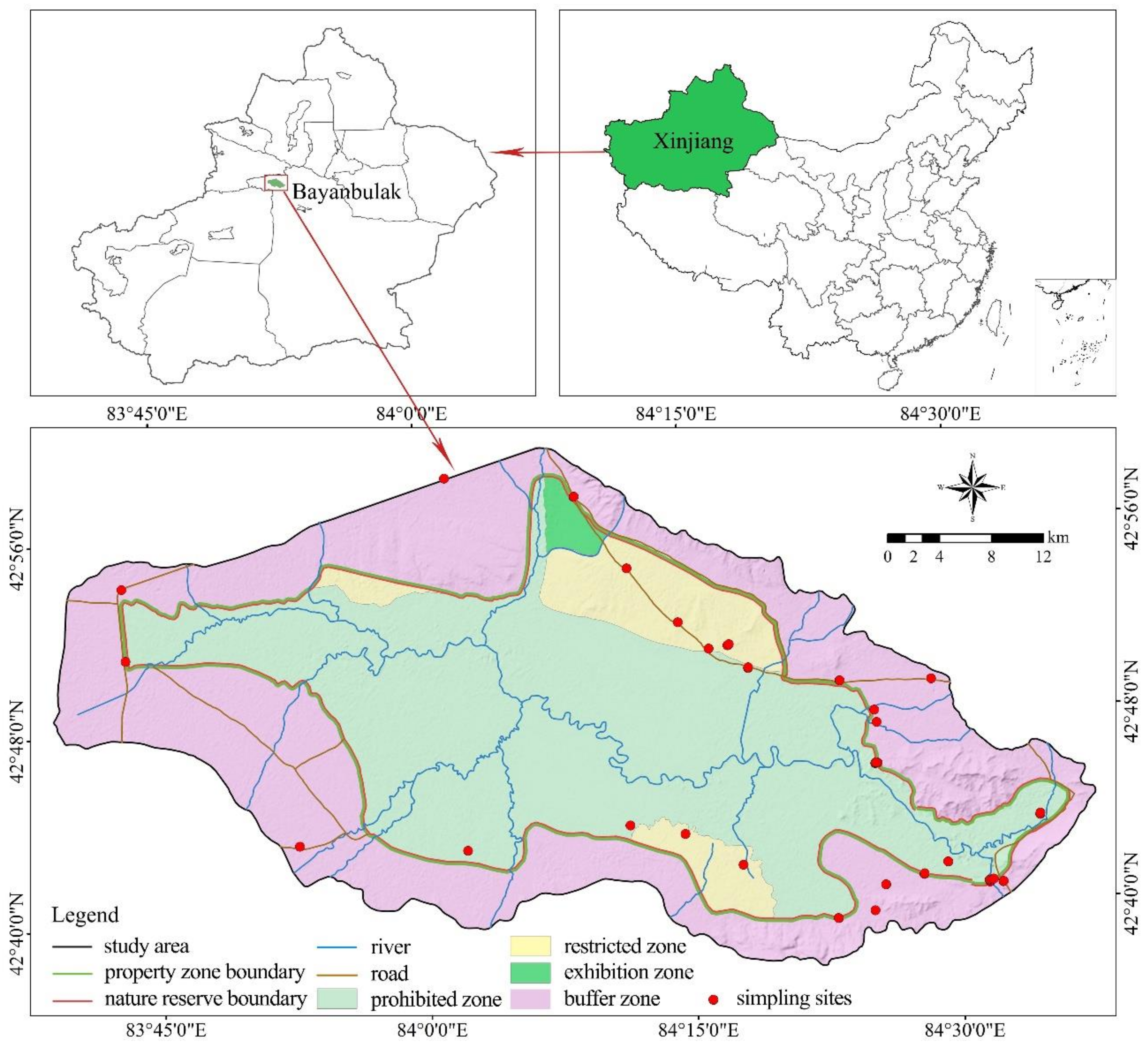
2.1. Study Area
2.2. Data Source and Processing
2.2.1. Data Sources
2.2.2. Data Processing
2.3. Method
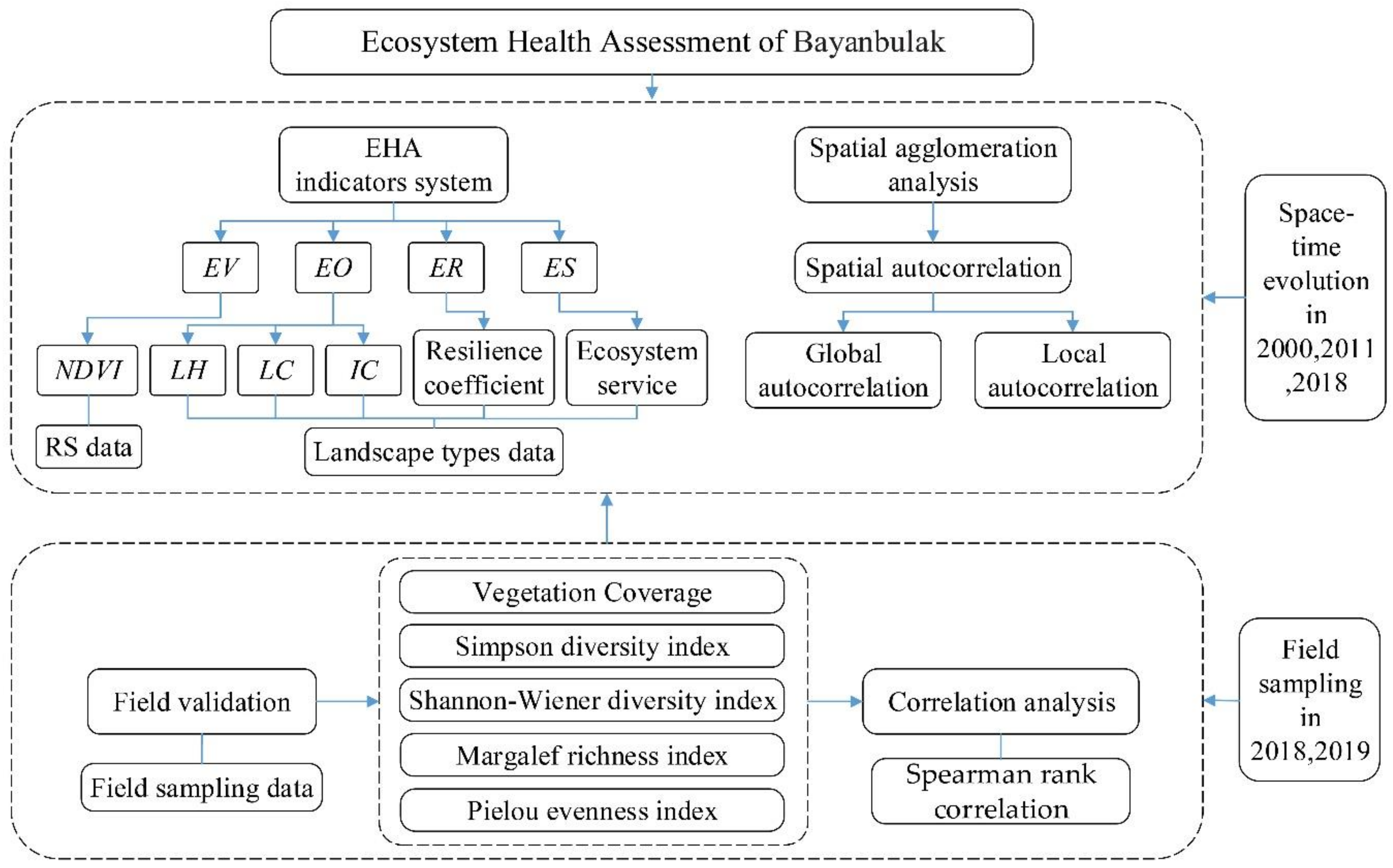
2.3.1. Ecosystem Health Assessment Framework
2.3.2. Ecosystem Health Assessment
- Ecosystem Health Assessment Model
- Ecosystem Health Assessment Indicators
2.3.3. Spatial Autocorrelation Analysis
2.3.4. Verification Based on Field Data
3. Results
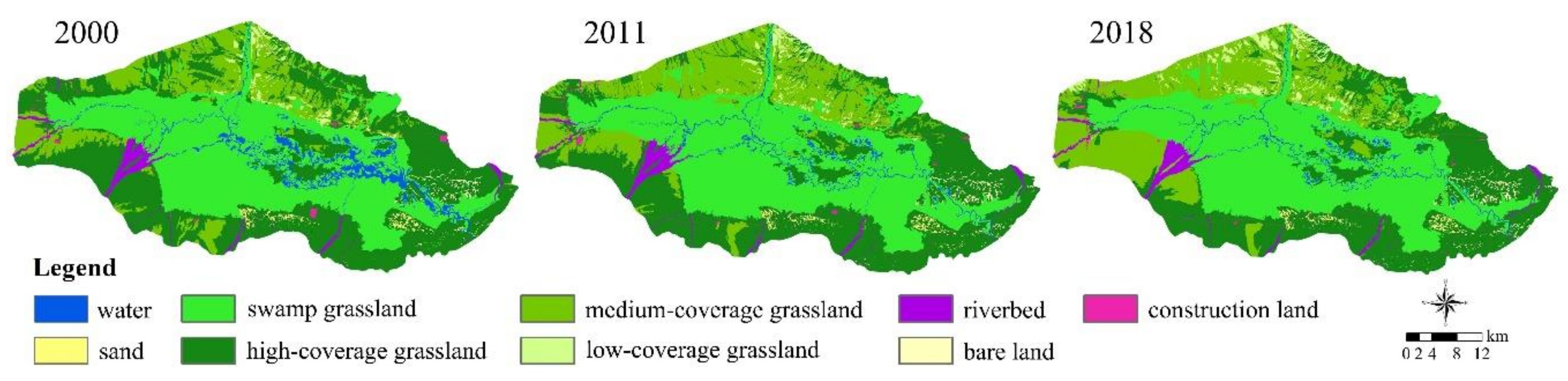
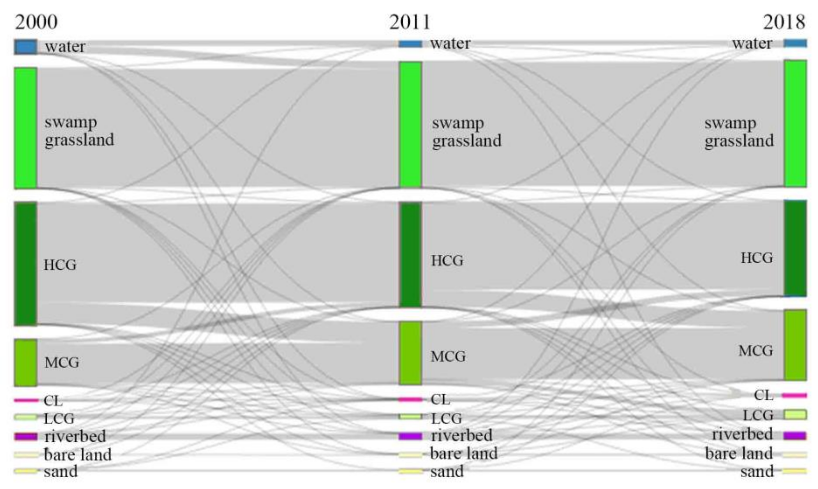
3.1. Changes in Ecosystem Landscape Types
3.2. Ecosystem Health Assessment
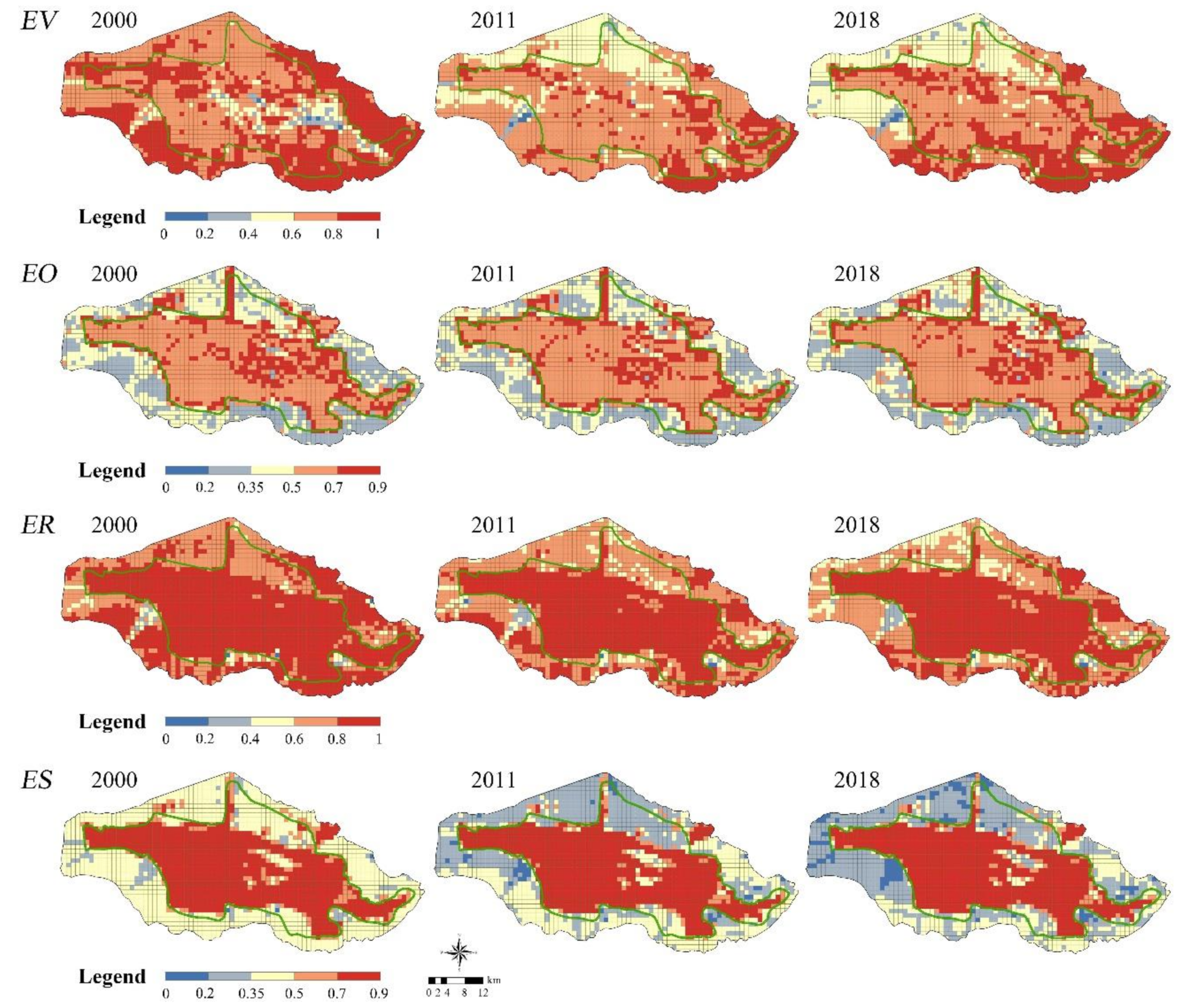
3.2.1. Changes in EHA indicators
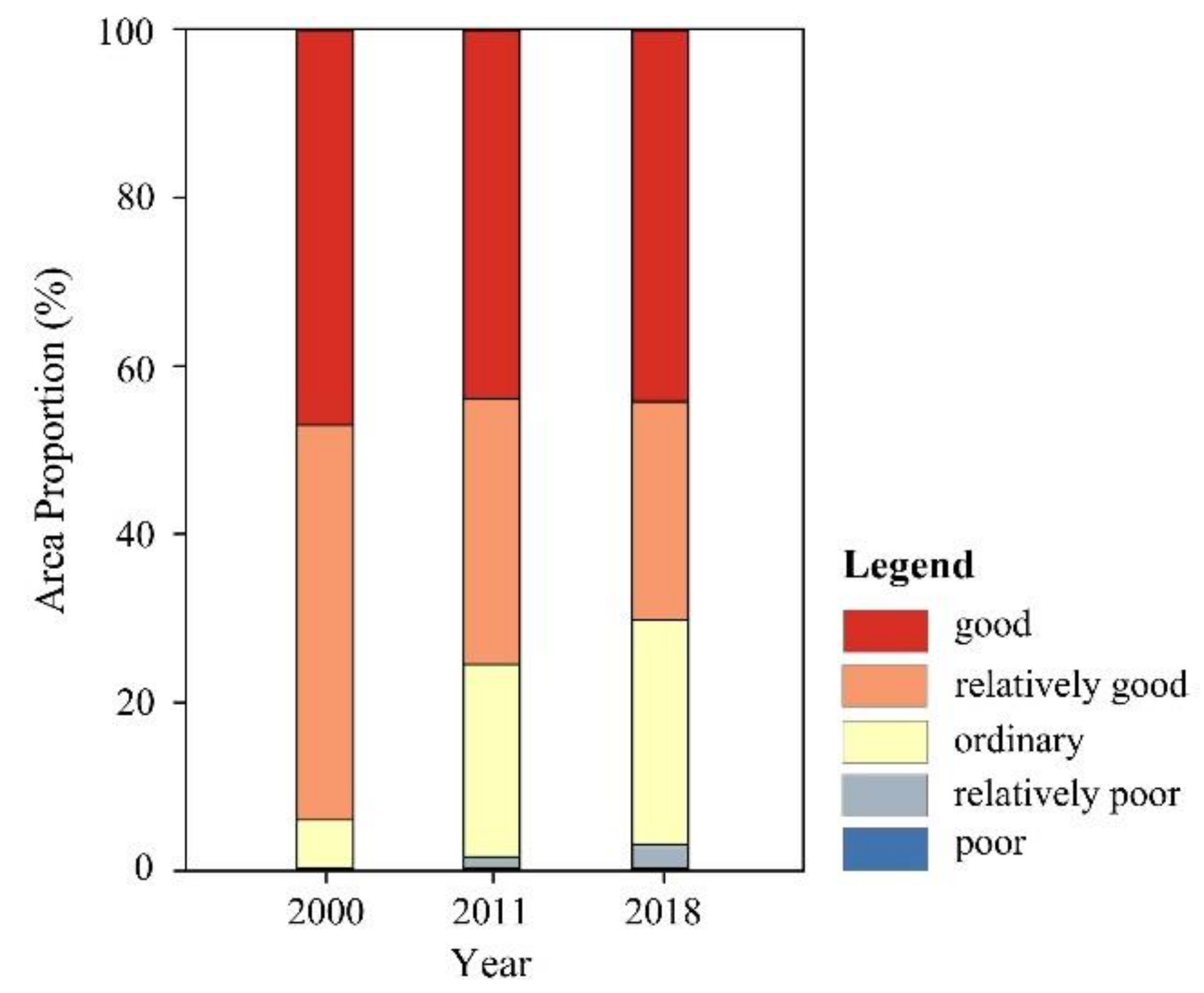
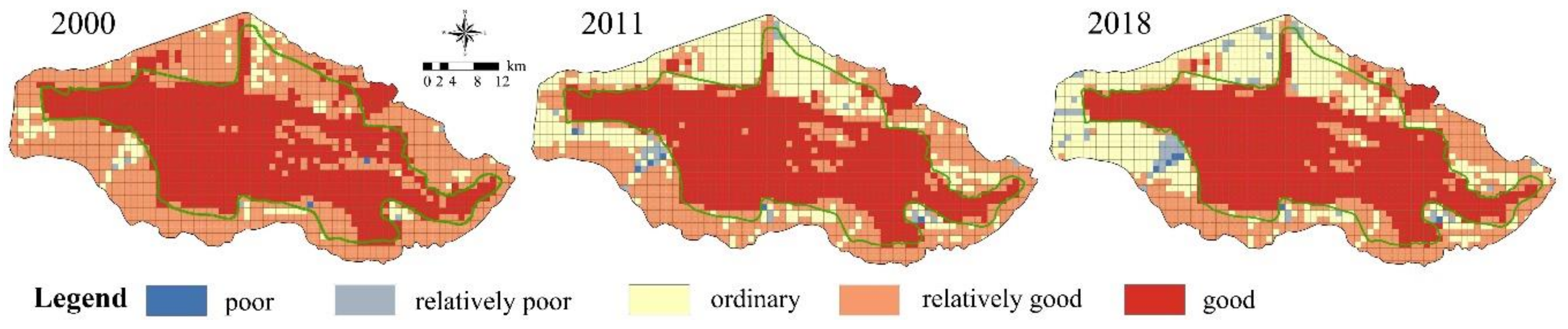
3.2.2. Changes in Ecosystem Health
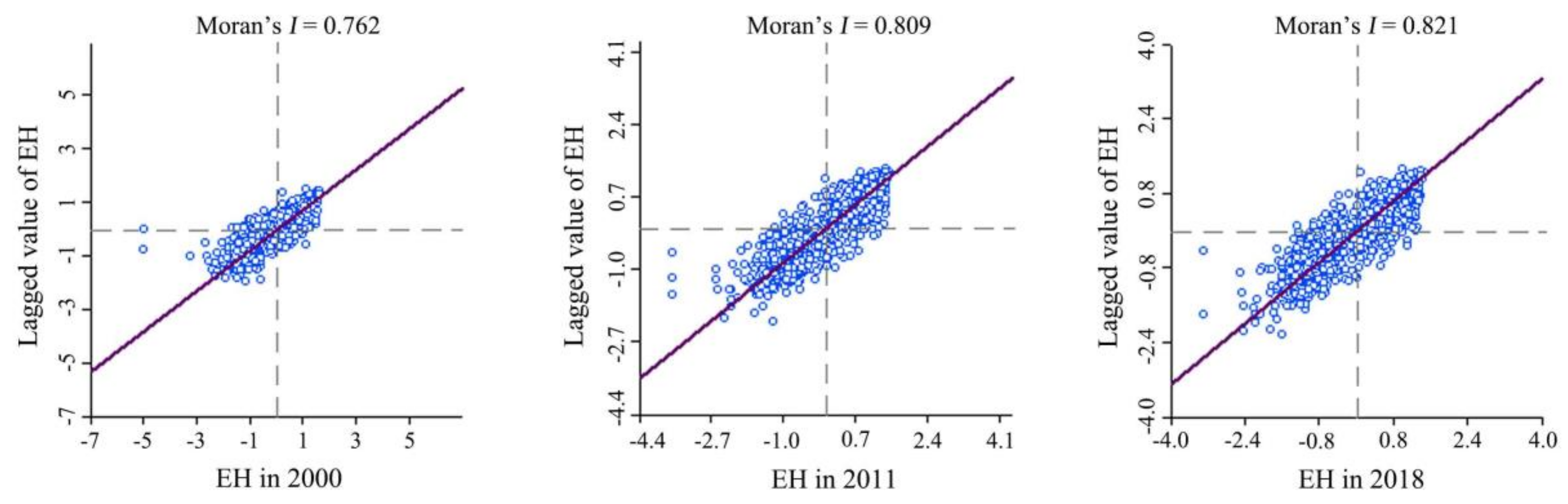
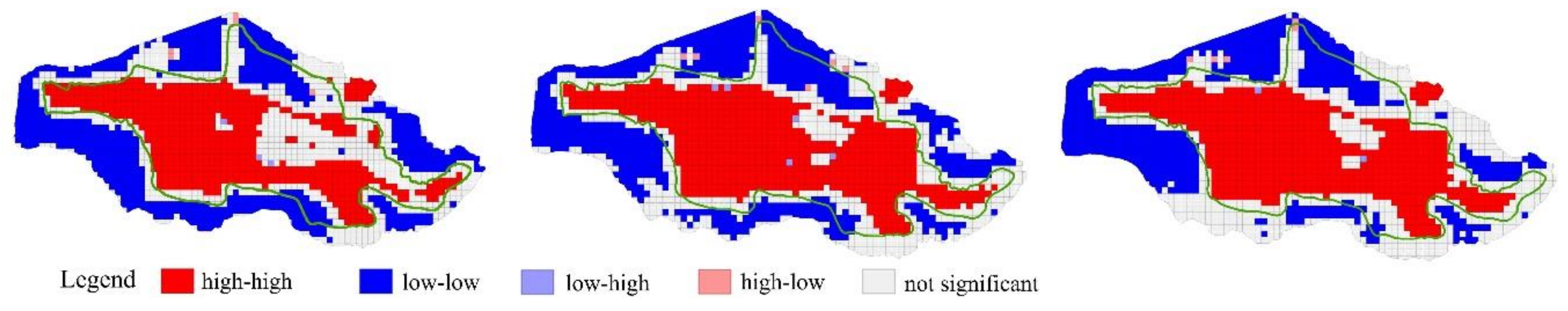
3.3. Spatial Autocorrelation Analysis
3.4. Field Verification
4. Discussion
4.1. Ecosystem Health Assessment model
4.2. Ecosystem Health Assessment
4.3. Limitations and Future Prospects
5. Conclusions
- While changes were observed in the area proportions of the various ecosystem landscape types from 2000 to 2018, the overall landscape structure did not change. The fragmentation of the landscape in the study area increased in general during the three periods. However, the degree of fragmentation remained small.
- All the EHA indicators showed a decline, with the decline in ES being the most significant. Thus, the overall ecosystem health in the study area also declined. However, the ecosystem health within the property zone remained high and essentially unchanged. Further, the area proportions of poor health were extremely low and were mostly distributed within the buffer zone. Therefore, in general, the ecosystem of the study area was in a healthy state.
- The spatial distribution of the ecosystem health exhibited obvious agglomeration characteristics, with the degree of agglomeration increasing over time. With respect to the local spatial autocorrelation, the high-high clusters were mainly distributed within the property zone, and the degree of agglomeration enhanced over time. On the other hand, the low-low clusters were mainly distributed in the buffer zone, and the degree weaken over time.
- The results of EHA obtained through RS monitoring were positively correlated with those of the field sampling of the vegetation in the study area. The areas with high levels of ecosystem health also exhibited high sampling vegetation index values. This confirmed the suitability of using RS imaging for monitoring ecosystem health.
Author Contributions
Funding
Acknowledgments
Conflicts of Interest
References
- UNESCO. Operational Guidelines for the Implementation of the World Heritage Convention; UNESCO: Paris, France, 2017. [Google Scholar]
- Jokilehto, J. World Heritage: Defining the outstanding universal value. City Time 2006, 2, 1. [Google Scholar]
- Wang, Z.; Yang, Z.; Du, X. Analysis on the threats and spatiotemporal distribution pattern of security in World Natural Heritage Sites. Environ. Monit. Assess. 2015, 187, 4143. [Google Scholar] [CrossRef]
- Allan, J.R.; Venter, O.; Maxwell, S.; Bertzky, B.; Jones, K.; Shi, Y.; Watson, J.E. Recent increases in human pressure and forest loss threaten many natural world heritage sites. Biol. Conserv. 2017, 206, 47–55. [Google Scholar] [CrossRef] [Green Version]
- UNESCO. Available online: http://www.unesco.org/ (accessed on 4 March 2020).
- Hedge, P.; Molloy, F.; Sweatman, H.; Hayes, K.R.; Dambacher, J.M.; Chandler, J.; Bax, N.; Gooch, M.; Anthony, K.; Elliot, B. An integrated monitoring framework for the great barrier reef world heritage area. Mar. Policy 2017, 77, 90–96. [Google Scholar] [CrossRef]
- Du, X.; Wang, Z. Optimizing monitoring locations using a combination of GIS and fuzzy multi criteria decision analysis, a case study from the Tomur World Natural Heritage site. J. Nat. Conserv. 2018, 43, 67–74. [Google Scholar] [CrossRef]
- Rapport, D.J.; Regier, H.A.; Hutchinson, T.C. Ecosystem behavior under stress. Am. Nat. 1985, 125, 617–640. [Google Scholar] [CrossRef]
- Costanza, R. Toward an operational definition of ecosystem health. In Ecosystem Health: New Goals for Environmental Management; Costanza, R., Norton, B.G., Hasktell, B.D., Eds.; Island Press: Washington, DC, USA, 1992; pp. 239–256. [Google Scholar]
- Rapport, D.J.; Costanza, R.; McMichael, A.J. Assessing ecosystem health. Trends Ecol. Evol. 1998, 13, 397–402. [Google Scholar] [CrossRef]
- Costanza, R. Ecosystem health and ecological engineering. Ecol. Eng. 2012, 45, 24–29. [Google Scholar] [CrossRef] [Green Version]
- Peng, J.; Liu, Y.; Wu, J.; Lv, H.; Hu, X. Linking ecosystem services and landscape patterns to assess urban ecosystem health: A case study in Shenzhen City, China. Landsc. Urban Plan. 2015, 143, 56–68. [Google Scholar] [CrossRef]
- Pan, Y.; Xu, Z.; Yu, C.; Tu, Y.; Li, Y.; Wu, J. Spatiotemporal variation of interacting relationships among multiple provisioning and regulating services of Tibet grassland ecosystem. Acta Ecol. Sin. 2013, 33, 5794–5801. [Google Scholar]
- Yang, W.; You, Q.; Fang, N.; Xu, L.; Zhou, Y.; Wu, N.; Ni, C.; Liu, Y.; Liu, G.; Yang, T.; et al. Assessment of wetland health status of Poyang Lake using vegetation-based indices of biotic integrity. Ecol. Indic. 2018, 90, 79–89. [Google Scholar] [CrossRef]
- Zhao, C.; Shao, N.; Yang, S.; Ren, H.; Ge, Y.; Zhang, Z.; Zhao, Y.; Yin, X. Integrated assessment of ecosystem health using multiple indicator species. Ecol. Eng. 2019, 130, 157–168. [Google Scholar] [CrossRef]
- Young, R.G.; Matthaei, C.D.; Townsend, C.R. Organic matter breakdown and ecosystem metabolism: Functional indicators for assessing river ecosystem health. J. N. Am. Benthol. Soc. 2008, 27, 605–625. [Google Scholar] [CrossRef]
- Xu, F.; Dawson, R.W.; Tao, S.; Cao, J.; Li, B. A method for lake ecosystem health assessment: An Ecological Modeling Method (EMM) and its application. Hydrobiologia 2001, 443, 159–175. [Google Scholar] [CrossRef]
- Liu, D.; Hao, S. Ecosystem health assessment at county-scale using the pressure-state-response framework on the Loess Plateau, China. Int. J. Environ. Res. Public Health 2017, 14, 2. [Google Scholar] [CrossRef] [Green Version]
- Sun, B.; Tang, J.; Yu, D.; Song, Z.; Wang, P. Ecosystem health assessment: A PSR analysis combining AHP and FCE methods for Jiaozhou Bay, China. Ocean Coastal. Manag. 2019, 168, 41–50. [Google Scholar] [CrossRef]
- Song, D.; Gao, Z.; Zhang, H.; Xu, F.; Zheng, X.; Ai, J.; Hu, X.; Huang, G.; Zhang, H. GIS-based health assessment of the marine ecosystem in Laizhou Bay, China. Mar. Pollut. Bull. 2017, 125, 242–249. [Google Scholar] [CrossRef]
- Suo, A.; Xiong, Y.; Wang, T.; Yue, D.; Ge, J. Ecosystem health assessment of the Jinghe River watershed on the Huangtu Plateau. EcoHealth 2008, 5, 127–136. [Google Scholar] [CrossRef]
- Wu, L.; You, W.; Ji, Z.; Xiao, S.; He, D. Ecosystem health assessment of Dongshan Island based on its ability to provide ecological services that regulate heavy rainfall. Ecol. Indic. 2018, 84, 393–403. [Google Scholar]
- Costanza, R.; De Groot, R.; Sutton, P.; Van der Ploeg, S.; Anderson, S.J.; Kubiszewski, I.; Farber, S.; Turner, R.K. Changes in the global value of ecosystem services. Glob. Environ. Chang. 2014, 26, 152–158. [Google Scholar] [CrossRef]
- Halpern, B.S.; Longo, C.; Hardy, D.; McLeod, K.L.; Samhouri, J.F.; Katona, S.K.; Kleisner, K.; Lester, S.E.; O’Leary, J.; Ranelletti, M.; et al. An index to assess the health and benefits of the global ocean. Nature 2012, 488, 615–620. [Google Scholar] [CrossRef] [Green Version]
- Meng, L.; Huang, J.; Dong, J. Assessment of rural ecosystem health and type classification in Jiangsu province, China. Sci. Total Environ. 2018, 615, 1218–1228. [Google Scholar] [CrossRef]
- De Toro, P.; Iodice, S. Ecosystem Health Assessment in urban contexts: A proposal for the Metropolitan Area of Naples (Italy). Aestimum 2018, 72, 39–59. [Google Scholar]
- He, J.; Pan, Z.; Liu, D.; Guo, X. Exploring the regional differences of ecosystem health and its driving factors in China. Sci. Total Environ. 2019, 673, 553–564. [Google Scholar] [CrossRef] [PubMed]
- Yan, Y.; Zhao, C.; Wang, C.; Shan, P.; Zhang, Y.; Wu, G. Ecosystem health assessment of the Liao River Basin upstream region based on ecosystem services. Acta Ecol. Sin. 2016, 36, 294–300. [Google Scholar] [CrossRef]
- Sun, T.; Lin, W.; Chen, G.; Guo, P.; Zeng, Y. Wetland ecosystem health assessment through integrating remote sensing and inventory data with an assessment model for the Hangzhou Bay, China. Sci. Total Environ. 2016, 566, 627–640. [Google Scholar] [CrossRef] [PubMed]
- Singh, P.K.; Saxena, S. Towards developing a river health index. Ecol. Indic. 2018, 85, 999–1011. [Google Scholar] [CrossRef]
- Chen, W.; Cao, C.; Liu, D.; Tian, R.; Wu, C.; Wang, Y.; Qian, Y.; Ma, G.; Bao, D. An evaluating system for wetland ecological health: Case study on nineteen major wetlands in Beijing-Tianjin-Hebei region, China. Sci. Total Environ. 2019, 666, 1080–1088. [Google Scholar] [CrossRef]
- Wu, N.; Liu, A.; Wang, Y.; Li, L.; Chao, L.; Liu, G. An Assessment Framework for Grassland Ecosystem Health with Consideration of Natural Succession: A Case Study in Bayinxile, China. Sustainability 2019, 11, 1096. [Google Scholar] [CrossRef] [Green Version]
- Xu, X.; Wang, X.; Zhu, X.; Jia, H.; Han, D. Landscape pattern changes in alpine wetland of Bayanbulak Swan Lake during 1996–2015. J. Nat. Resour. 2018, 33, 1897–1911. [Google Scholar]
- Zhang, M.; Xu, D.; You, G. Ecological carrying capacity and sustainable development of grassland and wetland in Bayanbulak national alpine grassland nature reserve. Biol. Disaster Sci. 2018, 41, 101–107. [Google Scholar]
- Lv, C.; Pan, X.; Feng, C.; Qian, J. Spectral models for estimating vegetation coverage and its application on Bayanbulak grassland. Bull. Soil Water Conserv. 2016, 36, 62–67. [Google Scholar]
- Shi, H.; Yang, Z.; Han, F.; Shi, T.; Li, D. Assessing landscape ecological risk for a world natural heritage site: A case study of Bayanbulak in China. Pol. J. Environ. Stud. 2015, 24, 269–283. [Google Scholar] [CrossRef]
- Liu, Q.; Yang, Z.; Han, F.; Shi, H.; Wang, Z.; Chen, X. Ecological environment assessment in world natural heritage site based on remote-sensing data. A case study from the Bayinbuluke. Sustainability 2019, 11, 6385. [Google Scholar] [CrossRef] [Green Version]
- Ayimin, B.; An, S.; Dong, Y.; Yang, J.; Zhang, A. Soil stoichiometry characteristics in different degradation stages of alpine steppe in Bayanbulak. Xinjiang Agric. Sci. 2018, 55, 957–965. [Google Scholar]
- Liu, Y. Ecological Factors of Pedicularis kansuensis Maxim. Expansion in Bayanbulak Grassland. Ph.D. Thesis, Xinjiang University, Urumqi, China, 2018. [Google Scholar]
- Yang, Z.; Zhang, X.; Xu, X.; Han, F.; Zhang, Y.; Yang, W.; Yan, S.; Hai, Y.; Yin, L.; Zhao, X.; et al. World Natural Heritage of Xinjiang Tianshan; Science Press: Beijing, China, 2017. [Google Scholar]
- Jia, H.; Cao, C.; Ma, G.; Bao, D.; Wu, X.; Xu, M.; Zhao, J.; Tian, R. Assessment of wetland ecosystem health in the source region of Yangtze, Yellow and Yalu Tsangpo Rivers of Qinghai province. Wetl. Sci. 2011, 9, 209–217. [Google Scholar]
- Peng, J.; Liu, Y.; Li, T.; Wu, J. Regional ecosystem health response to rural land use change: A case study in Lijiang City, China. Ecol. Indic. 2017, 72, 399–410. [Google Scholar] [CrossRef]
- Xiao, R.; Liu, Y.; Fei, X.; Yu, W.; Zhang, Z.; Meng, Q. Ecosystem health assessment: A comprehensive and detailed analysis of the case study in coastal metropolitan region, eastern China. Ecol. Indic. 2019, 98, 363–376. [Google Scholar] [CrossRef]
- Yu, G.; Yu, Q.; Hu, L.; Zhang, S.; Fu, T.; Zhou, X.; He, X.; Liu, Y.; Wang, S.; Jia, H. Ecosystem health assessment based on analysis of a land use database. Appl. Geogr. 2013, 44, 154–164. [Google Scholar] [CrossRef]
- Liao, C.; Yue, Y.; Wang, K.; Fensholt, R.; Tong, X.; Brandt, M. Ecological restoration enhances ecosystem health in the karst regions of southwest China. Ecol. Indic. 2018, 90, 416–425. [Google Scholar] [CrossRef]
- Yuan, M.; Liu, Y.; Wang, M.; Tian, L.; Peng, J. Ecosystem health assessment based on the framework of vigor, organization, resilience and contribution in Guangzhou City. Chin. J. Ecol. 2019, 38, 1249–1257. [Google Scholar]
- Xie, G.; Zhang, C.; Zhang, L.; Chen, W.; Li, S. Improvement of the evaluation method for ecosystem service value based on per unit area. J. Nat. Resour. 2015, 30, 1243–1254. [Google Scholar]
- Xie, G.; Zhang, C.; Zhen, L.; Zhang, L. Dynamic changes in the value of China’s ecosystem services. Ecosyst. Serv. 2017, 26, 146–154. [Google Scholar] [CrossRef]
- Mageau, M.T. The development and initial testing of a quantitative assessment of ecosystem health. Ecosyst. Health 1995, 1, 201–213. [Google Scholar]
- Myneni, R.B.; Ganapol, B.D.; Asrar, G. Remote sensing of vegetation canopy photosynthetic and stomatal conductance efficiencies. Remote Sens. Environ. 1992, 42, 217–238. [Google Scholar] [CrossRef]
- Phillips, L.B.; Hansen, A.J.; Flather, C.H. Evaluating the species energy relationship with the newest measures of ecosystem energy: NDVI versus MODIS primary production. Remote Sens. Environ. 2008, 112, 4381–4392. [Google Scholar] [CrossRef]
- Li, Z.; Xu, D.; Guo, X. Remote sensing of ecosystem health: Opportunities, challenges, and future perspectives. Sensors 2014, 14, 21117–21139. [Google Scholar] [CrossRef] [Green Version]
- Rapport, D.J. Ecosystem services and management options as blanket indicators of ecosystem health. J. Aquat. Ecosyst. Health 1995, 4, 97–105. [Google Scholar] [CrossRef]
- Turner, M.G. Landscape ecology: The effect of pattern on process. Annu. Rev. Ecol. Syst. 1989, 20, 171–197. [Google Scholar] [CrossRef]
- Frondoni, R.; Mollo, B.; Capotorti, G. A landscape analysis of land cover change in the Municipality of Rome (Italy): Spatio-temporal characteristics and ecological implications of land cover transitions from 1954 to 2001. Landsc. Urban Plan. 2011, 100, 117–128. [Google Scholar] [CrossRef]
- Kang, P.; Chen, W.; Hou, Y.; Li, Y. Linking ecosystem services and ecosystem health to ecological risk assessment: A case study of the Beijing-Tianjin-Hebei urban agglomeration. Sci. Total Environ. 2018, 636, 1442–1454. [Google Scholar] [CrossRef] [PubMed]
- Holling, C.S. Resilience and stability of ecological systems. Annu. Rev. Ecol. Syst. 1973, 4, 1–23. [Google Scholar] [CrossRef] [Green Version]
- Lautenbach, S.; Kugel, C.; Lausch, A.; Seppelt, R. Analysis of historic changes in regional ecosystem service provisioning using land use data. Ecol. Indic. 2011, 11, 676–687. [Google Scholar] [CrossRef]
- Costanza, R.; d’Arge, R.; De Groot, R.; Farber, S.; Grasso, M.; Hannon, B.; Limburg, K.; Naeem, S.; O’Neill, R.V.; Paruelo, J.; et al. The value of the world’s ecosystem services and natural capital. Nature 1997, 387, 253–260. [Google Scholar] [CrossRef]
- Xie, G.; Zhen, L.; LU, C.; Xiao, Y.; Chen, C. Expert Knowledge Based Valuation Method of Ecosystem Services in China. J. Nat. Resour. 2008, 23, 911–919. [Google Scholar]
- Moran, P.A. Notes on continuous stochastic phenomena. Biometrika 1950, 37, 17–23. [Google Scholar] [CrossRef]
- Anselin, L. Local indicators of spatial association—LISA. Geogr. Anal. 1995, 27, 93–115. [Google Scholar] [CrossRef]
- Quijas, S.; Schmid, B.; Balvanera, P. Plant diversity enhances provision of ecosystem services: A new synthesis. Basic Appl. Ecol. 2010, 11, 582–593. [Google Scholar] [CrossRef] [Green Version]
- Xie, H.; Wang, G.G.; Yu, M. Ecosystem multifunctionality is highly related to the shelterbelt structure and plant species diversity in mixed shelterbelts of eastern China. Glob. Ecol. Conserv. 2018, 16, e00470. [Google Scholar] [CrossRef]
- Shi, H.; Shi, T.; Han, F.; Liu, Q.; Wang, Z.; Zhao, H. Conservation value of world natural heritage site’ outstanding universal value via multiple techniques—Bogda, Xinjiang Tianshan. Sustainability 2019, 11, 5953. [Google Scholar] [CrossRef] [Green Version]
- Geng, S.; Shi, P.; Song, M.; Zong, N.; Zu, J.; Zhu, W. Diversity of vegetation composition enhances ecosystem stability along elevational gradients in the Taihang Mountains, China. Ecol. Indic. 2019, 104, 594–603. [Google Scholar] [CrossRef]
- Magurran, A.E. Ecological Diversity and its Measurement; Princeton University Press: Princeton, NJ, USA, 1988. [Google Scholar]
- Peng, J.; Wang, Y.; Wu, J.; Zhang, Y. Evaluation for regional ecosystem health: Methodology and research progress. Acta Ecol. Sin. 2007, 27, 4877–4885. [Google Scholar] [CrossRef]
- Mitchell, M.G.; Suarez-Castro, A.F.; Martinez-Harms, M.; Maron, M.; McAlpine, C.; Gaston, K.J.; Johansen, K.; Rhodes, J.R. Reframing landscape fragmentation’s effects on ecosystem services. Trends. Ecol. Evol. 2015, 30, 190–198. [Google Scholar] [CrossRef] [PubMed] [Green Version]
- Liu, R.; Dong, X.; Zhang, P.; Zhang, Y.; Wang, X.; Gao, Y. Study on the sustainable development of an arid Basin based on the coupling process of ecosystem health and human wellbeing under land use change—A case study in the Manas River Basin, Xinjiang, China. Sustainability 2020, 12, 1201. [Google Scholar] [CrossRef] [Green Version]
- Woodhill, J. Planning, Monitoring and Evaluating Programmes and Projects: Introduction to Key Concepts, Approaches and Terms; World Conservation Union: Gland, Switzerland, 2000. [Google Scholar]
- Job, H.; Becken, S.; Lane, B. Protected Areas in a neoliberal world and the role of tourism in supporting conservation and sustainable development: An assessment of strategic planning, zoning, impact monitoring, and tourism management at natural World Heritage Sites. J. Sustain. Tour. 2017, 25, 1697–1718. [Google Scholar] [CrossRef]
- Kruse, M. Ecosystem health indicators. In Encyclopedia of Ecology, 2nd ed.; Fath, B., Ed.; Elsevier: Amsterdam, The Netherlands, 2019; pp. 407–414. [Google Scholar]
- Ludwig, J.A.; Bastin, G.N.; Chewings, V.H.; Eager, R.W.; Liedloff, A.C. Leakiness: A new index for monitoring the health of arid and semiarid landscapes using remotely sensed vegetation cover and elevation data. Ecol. Indic. 2007, 7, 442–454. [Google Scholar] [CrossRef]
- Shi, Y.; Rui, H.; Luo, G. Temporal–Spatial distribution of ecosystem health and its response to human interference based on different terrain gradients: A case study in Gannan, China. Sustainability 2020, 12, 1773. [Google Scholar] [CrossRef] [Green Version]
- Qian, Y.; Lou, Y.; Chu, Y.; Liu, J.; Hu, J. Ecosystem Evaluation of International Important Wetlands in Dongting Lake. Wetl. Sci. 2016, 14, 516–523. [Google Scholar]
- Liu, Y.; Hu, Y.; Yu, J.; Li, K.; Gao, G.; Wang, X. Study on harmfulness of Pedicularis myriophylla and its control measures. Arid Zone Res. 2008, 25, 778–782. [Google Scholar]


| Indices | Indicators | Description | |
|---|---|---|---|
| EV | NDVI | EV refers to the primary productivity of the ecosystem. NDVI is widely used in ecosystem primary productivity evaluation. | |
| EO | landscape heterogeneity (LH) | Shannon’s diversity index (SHDI) | The higher the Shannon’s diversity index, the higher the heterogeneity, and the stronger the landscape organization. |
| Landscape connectivity (LC) | landscape fragmentation (FN) | Refers to the degree of landscape fragmentation, which reflects the spatial complexity of the landscape as a whole in the study area. | |
| connectivity of patches with important ecological functionality (IC) | Swamp grassland fragmentation (FN1) | Refers to the degree of swamp grassland landscape fragmentation, which reflects the complexity of landscape component space. | |
| swamp grassland patch cohesion index (COHESION) | The patch concentration index describes the natural connectivity of the corresponding patch type. The higher the patch concentration index, the better the connectivity, and the stronger the landscape organization. | ||
| ER | resilience coefficient | Set the resilience coefficient according to the resilience of different ecosystem types, the value is between 0–1. | |
| ES | ecosystem service value | Refer to Xie et al. (2015, 2017) to improve the value coefficient of terrestrial ecosystem services in China, and set the ecosystem service value of ecosystem types [47,48]. | |
| Ecosystem Type | Swamp Grassland | HCG | MCG | LCG | Water | Riverbed | Construction Land | Sand | Bare Land |
|---|---|---|---|---|---|---|---|---|---|
| RC | 0.9 | 0.8 | 0.7 | 0.6 | 0.8 | 0.5 | 0.2 | 0.1 | 0.2 |
| Service Type | Food Production | Raw Material | Water Supply | Gas Regulation | Climate Regulation | Purify Environment | Soil Maintenance | Biodiversity | Landscape Aesthetics |
|---|---|---|---|---|---|---|---|---|---|
| SWG | 1146.40 | 1123.93 | 5821.93 | 4270.92 | 8092.26 | 8092.26 | 5192.54 | 17690.59 | 10632.33 |
| HCG | 674.36 | 899.14 | 1775.80 | 3102.03 | 7395.43 | 3798.87 | 3776.39 | 6676.12 | 3664.00 |
| MCG | 539.48 | 719.31 | 1420.64 | 2481.63 | 5916.34 | 3039.09 | 3021.11 | 5340.89 | 2931.20 |
| LCG | 404.61 | 539.48 | 1065.48 | 1861.22 | 4437.26 | 2279.32 | 2265.83 | 4005.67 | 2198.40 |
| water | 1798.28 | 517.01 | 18634.68 | 1730.85 | 5147.58 | 12475.57 | 2090.50 | 5732.02 | 4248.44 |
| riverbed | 606.92 | 202.31 | 6226.55 | 674.36 | 1798.28 | 4473.22 | 809.23 | 2023.07 | 1461.10 |
| CL | 0.00 | 0.00 | 0.00 | 0.00 | 0.00 | 0.00 | 0.00 | 0.00 | 0.00 |
| sand | 22.48 | 67.44 | 44.96 | 247.26 | 224.79 | 696.83 | 292.22 | 269.74 | 112.39 |
| bare land | 0.00 | 0.00 | 0.00 | 44.96 | 0.00 | 224.79 | 44.96 | 44.96 | 22.48 |
| Landscape Type | Water | Swamp Grassland | Sand | HCG | MCG | LCG | Riverbed | Construction Land | Bare Land | Study Area |
|---|---|---|---|---|---|---|---|---|---|---|
| 2000 | 0.0058 | 0.0012 | 0.2439 | 0.0022 | 0.0076 | 0.0487 | 0.0083 | 0.0705 | 0.2448 | 0.0061 |
| 2011 | 0.0218 | 0.0010 | 0.2615 | 0.0048 | 0.0050 | 0.0868 | 0.0094 | 0.0525 | 0.2163 | 0.0076 |
| 2018 | 0.0367 | 0.0012 | 0.2754 | 0.0037 | 0.0051 | 0.0651 | 0.0120 | 0.0566 | 0.2369 | 0.0084 |
| Year | EV | EO | ER | ES | EH | |
|---|---|---|---|---|---|---|
| overall study area | 2000 | 0.7758 | 0.5431 | 0.8468 | 0.6507 | 0.6802 |
| 2011 | 0.6927 | 0.5397 | 0.8068 | 0.5820 | 0.6324 | |
| 2018 | 0.7000 | 0.5416 | 0.7956 | 0.5611 | 0.6251 | |
| property zone | 2000 | 0.7515 | 0.6377 | 0.9024 | 0.7928 | 0.7531 |
| 2011 | 0.7072 | 0.6345 | 0.8796 | 0.7544 | 0.7276 | |
| 2018 | 0.7400 | 0.6368 | 0.8794 | 0.7445 | 0.7330 | |
| buffer zone | 2000 | 0.8095 | 0.4560 | 0.7802 | 0.4881 | 0.6046 |
| 2011 | 0.6788 | 0.4529 | 0.7177 | 0.3826 | 0.5284 | |
| 2018 | 0.6638 | 0.4528 | 0.6952 | 0.3477 | 0.5075 |
| Vegetation Index | Good | Relatively Good | Ordinary | Relatively Poor |
|---|---|---|---|---|
| vegetation coverage | 92.22 ± 1.88 | 80.58 ± 5.28 | 72.90 ± 3.75 | 39.50 ± 5.5 |
| Simpson diversity index | 0.71 ± 0.04 | 0.64 ± 0.05 | 0.63 ± 0.02 | 0.53 ± 0.10 |
| Shannon-Wiener diversity index | 1.56 ± 0.12 | 1.43 ± 0.12 | 1.31 ± 0.07 | 1.12 ± 0.23 |
| Margalef richness index Pielou evenness index | 1.39 ± 0.17 0.68 ± 0.02 | 1.44 ± 0.16 0.63 ± 0.04 | 1.21 ± 0.11 0.65 ± 0.02 | 1.08 ± 0.08 0.60 ± 0.08 |
| Vegetation Index | rs | P value |
|---|---|---|
| vegetation coverage | 0.341 | 0.019 |
| Simpson diversity index | 0.323 | 0.035 |
| Shannon-Wiener diversity index | 0.318 | 0.038 |
| Margalef richness index | 0.170 | 0.277 |
| Pielou evenness index | 0.149 | 0.341 |
© 2020 by the authors. Licensee MDPI, Basel, Switzerland. This article is an open access article distributed under the terms and conditions of the Creative Commons Attribution (CC BY) license (http://creativecommons.org/licenses/by/4.0/).
Share and Cite
Wang, Z.; Yang, Z.; Shi, H.; Han, F.; Liu, Q.; Qi, J.; Lu, Y. Ecosystem Health Assessment of World Natural Heritage Sites Based on Remote Sensing and Field Sampling Verification: Bayanbulak as Case Study. Sustainability 2020, 12, 2610. https://doi.org/10.3390/su12072610
Wang Z, Yang Z, Shi H, Han F, Liu Q, Qi J, Lu Y. Ecosystem Health Assessment of World Natural Heritage Sites Based on Remote Sensing and Field Sampling Verification: Bayanbulak as Case Study. Sustainability. 2020; 12(7):2610. https://doi.org/10.3390/su12072610
Chicago/Turabian StyleWang, Zhi, Zhaoping Yang, Hui Shi, Fang Han, Qin Liu, Jianwei Qi, and Yayan Lu. 2020. "Ecosystem Health Assessment of World Natural Heritage Sites Based on Remote Sensing and Field Sampling Verification: Bayanbulak as Case Study" Sustainability 12, no. 7: 2610. https://doi.org/10.3390/su12072610