Economic Growth, Public and Private Investment: A Comparative Study of China and the United States

Abstract

Public and private investments play a central role in production functions by providing the required capital for development. There are many studies in the literature investigating the linear macroeconomic relations based on public and private investment in cross-country and country-specific analyses by focusing on various perspectives and methodologies. However, there is a gap in the literature in exploring nonlinear causal relations among public-private investment and economic growth, particularly in the U.S. and China, in order to comparatively discuss policy implementations and potential implications. To narrow the gap, this study investigates nonlinear causal relationships between public-private investment and gross domestic product in the U.S. and China, which are the largest economies comprising about 40 percent of the global gross domestic product (GDP) in 2018. These countries show a similar pattern in economic growth and implementing sustainable development goals, although they follow considerably different socio-economic regimes and fall into different development levels (i.e., developed and developing countries). Therefore, there should be a common underlying mechanism in macroeconomic factors that fosters economic development. In this regard, the motivation behind the study is to reveal a common, but hidden, behavior of the nonlinear causal relations of given macroeconomic factors in these countries to make recommendations about sustainable economic growth for policymakers. To this end, there are three main contributions of the paper. First, the research finds nonlinear dependencies in the related time series between 1960–2015, thereby nonlinear causality tests are performed to reach more reliable information than the linear causality. Second, the study formulates a feedback loop between public and private investment through economic growth, which indicates that public and private investment should stimulate each other directly or indirectly (i.e., through the GDP). Third, the direction of the causality does not affect sustainable economic growth as long as it exists directly or indirectly.

1. Introduction

Economists have long discussed how to predict global and country-specific market fluctuations, recessions, economic turmoil, and financial crises, and how to correct these problems for the welfare of nations. Therefore, many macroeconomic factors have been investigated to find a robust model and framework explaining past performance and determining the future behavior of the economies. In this regard, investment and economic growth have been studied by many researchers in the literature since the late 1970s, describing the change in the macroeconomic dynamics, particularly, in both developed and developing countries. There is a complex relationship between public-private investment and economic growth. They affect each other and depend on many external factors such as the capacity of human resources [1], geographical and cultural conditions [2], natural resources, income taxation [3,4], debt-based investing [5], and the political regimes [6]. This study investigates the interrelations of public-private investment and economic growth in the U.S. and China in order to reveal nonlinear causal relations and comparatively discuss policy implementations and potential implications.

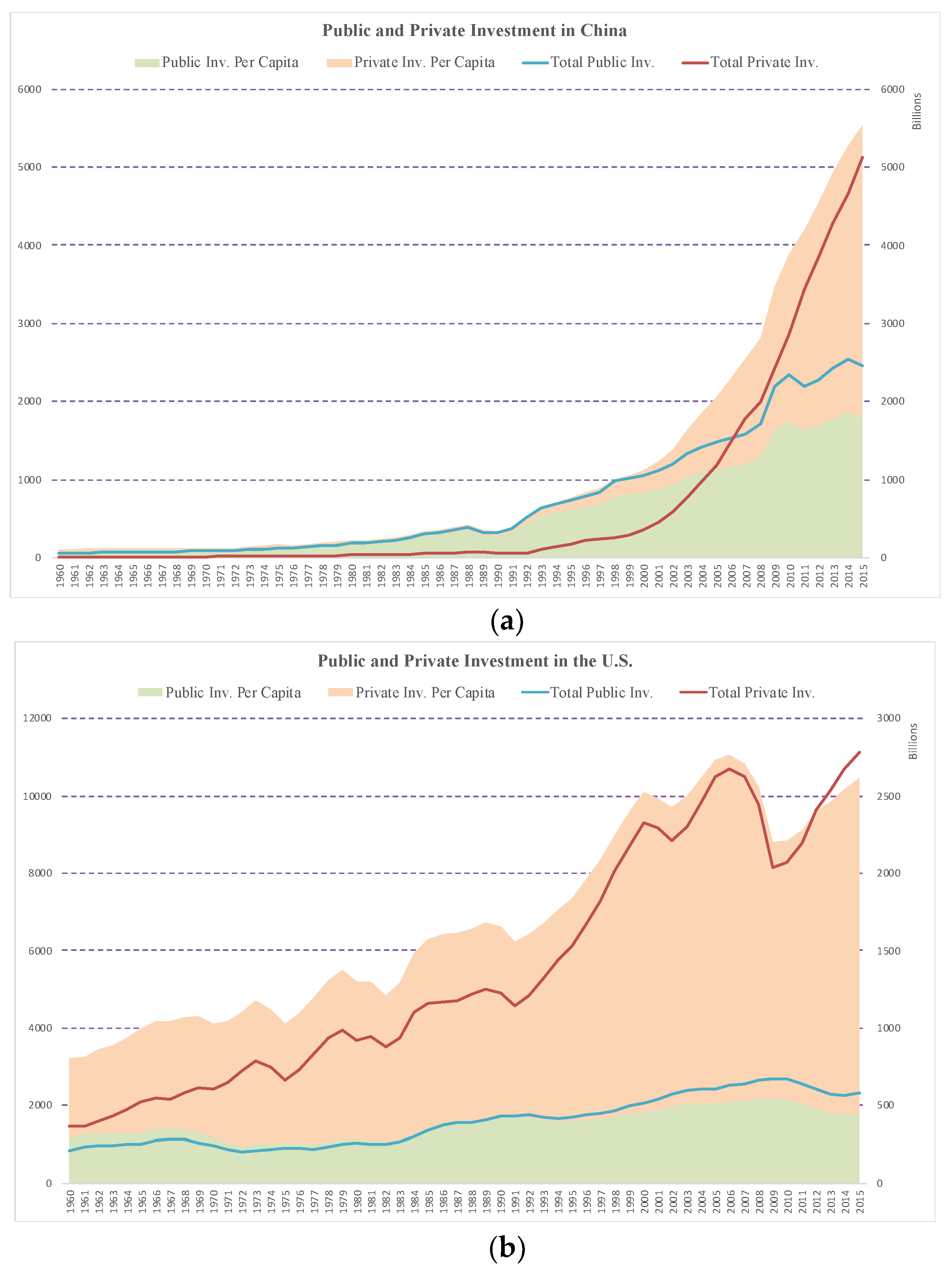
Public and private investment data represent different behavior in both countries (see Figure 1). In both countries, public investment per capita (PUC) reached about USD 1800 in 2015, although they arrived at this point by following very different trends. The U.S. PUC has been increased by only 50% between 1960 and 2015, while there has been a dramatic rise in China by twenty times in the same period. Private investment per capita (PRIC) in the U.S. has grown by four times between 1960 and 2015, although there have been fluctuations over the course. It has been higher than the PUC in the U.S. at all times. PRIC in the U.S. reached about USD 8500 in 2015, that is, more than twice the value in China. However, China has made significant progress by dramatically increasing the PRIC by more than 200 times for the same period. There has been a steep rise in the PRIC in China after 1992, and it exceeded the PUC of China in 2006. This rapid progress after the 1990s is because China implemented new policies that opened up the economy to foreign investment and performed an unprecedented system that enabled free enterprise and capitalist ideas within a socialist framework to grow economy and social welfare under the control of a single-party political system. In short, public and private investment has shown a similar pattern in 2015, at the end of the data points, although they have followed considerably separate routes.

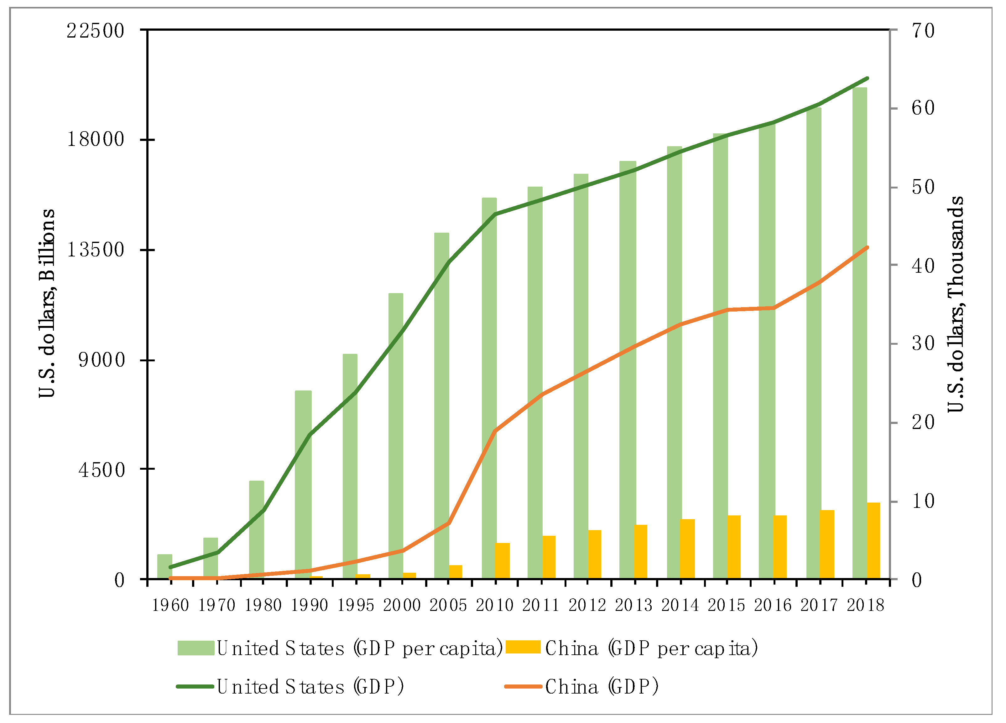
The U.S. and China, which are the largest economies comprising about 40 percent of the global gross domestic product (GDP) in 2018, show a remarkably similar trend in economic growth in the last 20 years (see Figure 2), although they follow considerably different socio-economic regimes. Figure 2 also shows that these countries fall into different levels of development in terms of the GDP per capita. In other words, regarding the GDP per capita, the U.S. and China produce more than USD 60 thousand and less than USD 10 thousand in 2018, respectively, which indicates the former is considered as a developed country and the latter is developing one. Therefore, the similarities of economic growths in both countries enabled us to ask the key question: What might be a common framework in sustaining economic growth for the U.S. (a developed country) and China (a developing country) in terms of public and private investment? This study answers the question and proposes a policy framework for sustainable economic growth. The motivation behind the study is to reveal a common, but hidden, behavior of the nonlinear causal relations of given macroeconomic factors in these countries to make recommendations about sustainable economic growth for policymakers. To this end, there are three main contributions of the paper. First, the research finds nonlinear dependencies in the related time series between 1960–2015, thereby nonlinear causality tests are performed to reach more reliable information than the linear causality. Second, the study formulates a feedback loop between public and private investment through economic growth, which indicates that public and private investment should stimulate each other directly or indirectly (i.e., through the GDP). Third, the direction of the causality does not affect sustainable economic growth as long as it exists directly or indirectly.

2. Literature Review

The investment and economic growth have been studied by many researchers for both developing and developed countries since the late 1970s. Buiter [9] discussed the idea that public capital for infrastructure has an impact on private investment and economic growth. He advocated the existence of a complementary relationship between public and private investment. Later, the component of public investment had remained hidden or ignored in the analyses of productivity growth until the study by Aschauer [10]. He initiated a long-unsettled dialog between politicians and economists by arguing that much of the decline in U.S. productivity during the 1970s was estimated by reducing rates of public investment. Aschauer [10] drew attention to the significance of public capital for infrastructure by embedding public investment into the conventional production function [10]. This indicates that public investment policy exerts a great influence on the course of national (i.e., public and private) capital accumulation and economic growth, and such fiscal policy is considered as ‘nonneutral’ regarding the progress of the private sector. These findings were further supported by Munnell [11] and Greene and Villanueva [12]. There were also sharp criticisms against the complementary relationship by such as Tatom [13] and Evans and Karras [14], who found that public investment has a negligible effect on productivity.

Erenburg [15] approached the problem from a different perspective by embedding both public capital stock and government investment spending in various investment models to investigate the change in private investment activity. He obtained a statistically significant inverse relationship between private investment activity and public investment flow but a direct relationship with public capital stock. Put differently, neglecting public investment for infrastructure has an adverse effect on private sector equipment investment and economic growth. In the following study, Erenburg and Wohar [16] studied the causal linkage among private investment and public capital stock and government investment spending. They found that there is a feedback effect between public and private investment rather than a unidirectional causality. However, Voss [17] examined private and public investment by employing an unstructured vector autoregression (VAR) model and found a conflicting result that there is no ‘crowding in’ effect due to complementarities between public and private investment. Erden and Holcombe [18] investigated the relationship between public and private investment by applying an investment model to panel data of developed and developing countries. Their result revealed that public investment crowds in private investment in developing countries while crowding out private investment in developed countries. This might be because public investment provides the required infrastructure facilities in emerging economies that promote private investment; on the other hand, the developed economies have a mature public sector, and more investment might cause resource scarcity or compete with the private sector.

Mittnik and Neumann [19] investigated the causal relationship between public investment and economic growth for six developed countries by examining impulse responses derived from vector autoregressions. Their empirical findings showed that public investment inclines to apply a positive impact on the GDP. To measure the level of public investment required for economic growth, Barro [20] derived a growth-maximizing spending share by utilizing an endogenous-growth model that combines productive public investment into the production function. He illustrated that the growth-maximizing share acts as a limit for promoting economic growth and determines the relationship between public spending and growth. In other words, additional public investment will raise economic growth when it is under the growth-maximizing share.

Xu and Yan [21] demonstrated the impact of public investment on private investment in China by dividing public investment into the spending on public goods and private industry. Their findings suggested that public investment in public goods promotes private investment significantly, while government spending in private industry discourages private investment significantly. Furthermore, Dreger and Reimers [22] explored the long-run relationship between public and private investment by applying econometric panel models for Europe. They presented that public investment scarcity might limit private investment and economic growth in Europe. Bahal et al. [23] followed a different angle for investigating the relationship between public and private investment by dividing the time series into two chunks, before and after 1980. They found that public investment discourages private investment in India over the entire sample, whereas the opposite is correct when the sample is restricted to post 1980. They attributed this feature to the policy changes after the 1980s.

Ari et al. [24] analyzed the nonlinear relationship between public and private investment for the hydrocarbon-based rentier states in the case study of GCC countries. They illustrated that public investment leads to private investment in those countries because of the lack of economic diversification. Afonso and St. Aubyn [25] investigated the economic growth effects of public and private investment in seventeen OECD countries by a linear VAR analysis. They found that public investment crowded-in economic growth in many countries and crowded-out in Japan, UK, Canada, Sweden, and Finland. Besides, they showed that private investment induced a positive growth path in all sample countries. Deleidi et al. [26] examined the macroeconomic effect of public investment on economic growth in eleven Eurozone countries by Local Projections (LP) methodology, which is an alternative model to VAR models. They presented that an increase in public investment promotes economic growth both in the short and long run. Masten and Grdović Gnip [27] studied the dynamic effects on macroeconomic implications of public investment in South-East Europe by the LP methodology. They also confirmed that public investment had a positive effect on GDP and private investment. Besides, they also noted that the countries in their study have low (less than 60%) public debt-to-GDP ratio. Abdul et al. [28] emphasized that public investment demonstrates higher efficiency and boosting productivity when it is a debt-based investment. However, Ari and Koc [29] provided a piece of evidence for the claim in the U.S., China, Japan, and Germany that an increase in public debt-to-GDP retards public investment if it exceeds certain limits. In this case, Ari and Koc [30] developed a novel financing model to reduce debt-based financing for public investment through private participation.

In summary, there are many studies in the literature investigating the interrelations among economic growth, public investment and private investment with various methods such as embedding these variables into production function, employing various investment models, and performing causality tests. However, there is a gap in studying nonlinear interrelations between the three variables (public and private investment, and economic growth) to establish a structure, such as a feedback loop, in China and the United States. This paper narrows this gap by three main contributions. First, the research finds nonlinear dependencies in the related time series between 1960–2015, thereby nonlinear causality tests are performed to reach more reliable information than the linear causality. Second, the study formulates a feedback loop between public and private investment through economic growth, which indicates that public and private investment should stimulate each other directly or indirectly (i.e., through the GDP). Third, the direction of the causality does not affect sustainable economic growth as long as it exists directly or indirectly.

3. Methodology

3.1. Data

Gross domestic product (GDP) is a widely utilized measure of a country’s overall economic activity, and the change in GDP corresponds to economic growth. This study gathers the GDP data of the U.S. and China from the International Monetary Fund (IMF) [8]. Public and private investment might have an influence on sustainable economic growth. Public investment can be considered a source that provides physical assets for the benefit of the public by providing economic infrastructure (such as highways, railways, seaports, airports, and power plants) and social infrastructure (such as schools, universities, and hospitals). Private investment, on the other hand, is recognized as profit-driven financing by private entities in order to maximize their benefits. In this study, public and private investments span the time between 1960 and 2015. The data is collected from the IMF Fiscal Affairs Department [31,32]. All variables collected in this study are expressed in the logarithm for analysis.

3.2. The Unified Causality Framework

This study designs a unified framework for statistical experiments conducted in the research to systematically investigate the nonlinear causality and devise a policy framework for sustainable economic growth. The causality framework consists of three stages that are pretesting, linear causality, and nonlinear causality (see Figure 3).

In the pretesting stage, the Augmented Dickey-Fuller (ADF) and Zivot-Andrew (ZA) unit root tests (URTs) are conducted to obtain integration orders (in levels or first differences) of the variables for public and private investment and economic growth [33,34]. The reason for performing more than one URT for the same time series, rather than depending on the results from only one test, is to crosscheck the integration orders for the same dataset. Put differently; URTs cannot calculate integration orders with a hundred percent certainty, therefore, conducting various URTs for the same dataset increases the accuracy of the integration orders. This research consolidates integration orders from various URTs for the same time series by confirmation analysis. If the ADF and ZA tests give the same integration order for the same time series, then confirmation analysis shows a conclusive result, and this series can be considered as a stationary dataset. Otherwise, the confirmation analysis leads to a nonconclusive result indicating that the time series is not a stationary dataset and thereby, not appropriate for Granger causality [35]. Next, in the pretesting stage, the Johansen cointegration test is conducted to evaluate the long-run relationship for the given datasets by investigating whether the time series share a common trend or not [36]. The existence of cointegration indicates that there exists a long-run relationship among variables, but this test cannot reveal the direction of the interrelation. To determine the direction, the study follows the next stage in the unified framework, which is the linear causality stage.

In the linear causality stage, the study examines the conditions that resulted in the pretesting stage. If the time series is stationary and there is no pairwise cointegration, then the linear causality is examined by the Granger test. If the condition is not satisfied, then the Toda-Yamamoto Granger test is performed for further analysis of the linear causality. In the last step, the BDS test is conducted to ascertain the existence of the nonlinear behaviors in the given time series. The nonlinearity test is performed for variables when the null hypothesis of the BDS, which is a series of independent and identically distributed random variables, is rejected [37]. In the case of the nonlinearity in a given time series, the study performs the nonlinear Granger causality test.

3.3. Confirmatory Analysis

The ADF and ZA tests are performed to discover the integration orders in a given dataset. The reason for employing more than one analysis in finding the integration order is that unit root tests rarely provide different conclusions from each other. Therefore, the research conducts confirmatory analysis to crosscheck the stationarity of a given time series and enhance the accuracy of the conclusion of whether each dataset is stationary. The confirmatory analysis consolidates integration orders from the ADF and ZA tests for the same dataset. If both tests result in an identical integration order, then the confirmation analysis provides a conclusive result, and this series can be considered as a stationary time series. Otherwise, the confirmation analysis leads to a nonconclusive result that the time series is a non-stationary time indicating the appropriateness of the standard Granger causality. Otherwise, the confirmation analysis leads to a nonconclusive result, whether the time series is stationary or not. If all the variables become stationary in levels or differences, then confirmatory analysis compares the integration orders of the variables pairwise before conducting causality tests between them. The dependent and independent variables in a causality test have a common integration order if the orders in a pairwise comparison of the variables are identical. Otherwise, the confirmatory analysis leads to a nonconclusive result indicating that the standard Granger causality is not an appropriate test. In this case, after performing the Johansen cointegration test for examining the long-run relationship, the study conducts the Toda-Yamamoto (TY) Granger causality.

3.4. Toda-Yamamoto (TY) Causality Test

The causality tests carry crucial importance in modeling a country’s economic system for policymaking because this relationship defines the direction and amount of the flow data and the behaviors of the agents in the model. The Granger test has a couple of limitations depending on datasets that lead the test to unreliable results. There are two primary conditions checked right after the pretesting stage in this study to reach reliable conclusions. First, the pairwise datasets associated with the Granger causality have to become stationary in the same integration order with each other. The confirmatory analysis examines this condition in the pretesting stage and finds that this requirement is satisfied for performing the Granger test. To avoid spurious results, the second condition is to have no cointegration between the variables that are subjected to test the causality. In this regard, the Granger test is not applicable for analyzing the causality in this study because all variables are cointegrated pairwise. In detail, Toda and Phillips [38] demonstrated the limitations of the Granger test.

Toda and Yamamoto [39] derived a reliable approach that is based on the Wald test running on the augmented VAR (p + d_max) model, where d_max is the maximum integration order between the variables under the pairwise causality test. Thus, the Wald statistic converges to the asymptotic χ² random variable. Additionally, this test does not require any pretesting conditions between pairwise variables to avoid spurious results. The augmented VAR (p + d_max) model for TY Granger causality is represented as follows:

$$Y_t=\widehat{\gamma }+\widehat{C_1}{Y}_{t-1}+\cdots +\widehat{C_p}{Y}_{t-p}+\widehat{C_{p+d_{max}}}{Y}_{t-p-d_{max}}+\widehat{u_t}$$

(1)

where the circumflex over $C_k$, $\gamma$, and $u_t$ expresses the estimation of ordinary least squares; $C_k$ denotes the $nxn$ matrix for lag k ($k=1,\dots ,p$); d_max represents the maximum integration in pairwise variables. This study calculates the lag order $p$ by the Schwarz Information Criterion (SIC) [40]. In the Wald test based on the augmented VAR (p + d_max), if the null hypothesis H₀ is rejected, then the jth element of $Y_t$ does Granger-cause the ith element of $Y_t$.

$$H_0:\mathrm{The}\left(i,j\right)\mathrm{element}\mathrm{of}{C}_k\mathrm{equals}\mathrm{zero}\mathrm{for}k=1,\dots ,p.$$

The TY Granger test requires that the lag $p$ has to be greater than or equal to $d_{max}$ of the variables unless there is cointegration between the variables [39].

3.5. BDS Nonlinearity Test

This test utilizes the concept of the correlation integral [41] to investigate the “identically and independently distributed (henceforth, called as i.i.d.)” assumption on the error term. The correlation integral for an m-dimensional variable $X_t$, where m represents embedding dimensions, is given as follows [42]:

$$C_m\left(T,ϵ\right)=\frac{2}{T_m\left(T_{m-1}\right)}\times {\displaystyle \sum _{t=1}^{T_m-1}\sum _{s=t+1}^{T_m}}I\left(X_t^m,X_s^m,ϵ\right)$$

(2)

here $\left(X_t,X_{t+1},\dots ,X_{t+m-1}\right)$ are the observations. $I\left(X_t^m,X_s^m,ϵ\right)$ denotes the indicator function below:

$$I\left(X_t^m,X_s^m,ϵ\right)=\{\begin{array}{llll}1,& & & if\Vert X_t^m,X_s^m\Vert <ϵ\\ 0,& & & otherwise\end{array}$$

(3)

where $\Vert X_t^m,X_s^m\Vert$ corresponds to the Euclidian distance between $X_t^m$ and $X_s^m$, $T$ represents the size of the sample, and $T_m$ denotes the sub-sample size for the m dimensions. Brock et al. (1996) derived the BDS statistic as follows [43]:

$$W_m\left(T,ϵ\right)=\frac{\sqrt{T}\left(C_m\left(T,ϵ\right)-C_1{\left(T,ϵ\right)}^m\right)}{{\sigma }_m\left(ϵ\right)}$$

(4)

where $ϵ$ is a radius of the bandwidth, and ${\sigma }_m\left(ϵ\right)$ denotes the standard deviation for the m-dimensional sample. This statistic asymptotically converges to the standard normal distribution. In the BDS test, if the null hypothesis H₀ is rejected, then there exists a nonlinearity in a time series.

$$H_0:X_t\mathrm{is}\mathrm{a}\mathrm{series}\mathrm{of}\mathrm{i}.\mathrm{i}.\mathrm{d}.\mathrm{random}\mathrm{variables}.$$

3.6. Nonlinear Granger Causality

Time-series might follow complex and hidden behaviors whereby linear tests cannot uncover the causality. Baek and Brock [44] (BB), therefore, derived a nonlinear test for the causality based on the Granger test. Hiemstra and Jones [45] (HJ) improved the BB test by decreasing problems in nuisance-parameter and increasing sizes and power properties of the finite-sample. Diks and Panchenko [46] showed that the HJ test has a propensity for over-rejection of the null hypothesis. In the same study, they derived nonparametric test statistics (henceforth, called the DP test) for the causality based on the Granger test. The HJ test statistic is replaced with a weighted average of local contributions. Then, the DP test changed the null hypothesis to the local conditional mean given in Equation (5).

$$H_0:E\left[f_{X,Y,Z}\left(X,Y,Z\right)f_Y\left(Y\right)-f_{X,Y}\left(X,Y\right)f_{Y,Z}\left(Y,Z\right)\right]=0$$

(5)

The natural estimator of $H_0$ utilizing the indicator function in Equation (3) is shown as follows.

$$T_n\left({ϵ}_n\right)=\frac{{\left(2ϵ\right)}^{-d_x-2d_y-d_z}}{n\left(n-1\right)\left(n-2\right)}{\displaystyle \sum _i}\left[{\displaystyle \sum _{k,k\ne i}\sum _{j,j\ne i}}{I}_{ik}^{XYZ}{I}_{ij}^Y-I_{ik}^{XY}{I}_{ij}^{YZ}\right]$$

(6)

This statistic indicates the average value of Equation (4) for the conditional distributions of X and Z, given $Y\ne y_i$.

The null hypothesis can be reformulated by the invariant distribution of $W_t=(X_t^{l_x},Y_t^{l_y},Y_{t+1})$. Assuming that $W_t$ is a continuous random variable, then it becomes $W=\left(X,Y,Z\right)$ by removing the time index $t$ and by taking $l_x=l_y=1$. Following this simplification, the local density function, which is the estimator of a $d_W$-variate random vector is given as follows;

$$\widehat{f_W}\left(W_i\right)=\frac{{\left(2ϵ\right)}^{-d_W}}{n-1}{\displaystyle \sum _{j,j\ne i}}{I}_{ij}^W$$

(7)

then the test statistic can be derived from Equation (7) as follows:

$$T_n\left({ϵ}_n\right)=\frac{n-1}{n\left(n-2\right)}{\displaystyle \sum _i}\left(\widehat{f_{X,Y,Z}}\left(X_i,Y_i,Z_i\right)\widehat{f_Y}\left(Y_i\right)-\widehat{f_{X,Y}}\left(X_i,Y_i\right)\widehat{f_{Y,Z}}\left(Y_i,Z_i\right)\right)$$

(8)

Diks and Panchenko [46] proved that the statistic in Equation (8) prevents the over-rejection under various bandwidths ${ϵ}_n$

$$\frac{\sqrt{n}\left(T_n\left({ϵ}_n\right)-q\right)}{S_n}\stackrel{converges}{\to }N\left(0,1\right)$$

(9)

where $S_n$ denotes the estimator of the asymptotic standard deviation of $\sqrt{n}\left(T_n\left({ϵ}_n\right)-q\right)$. This study performs the nonlinear Granger-causality test by using the DP test statistic.

4. Empirical Results and Discussions

4.1. Unit Root Tests

This study, first examines whether the variables are stationary in levels or first differences by conducting unit root tests—the ADF and ZA. These tests are required to determine the following methodology for conducting causality tests. Besides, the ZA test also delivers the structural time breaks in variables, which shows dramatic changes in a given time series.

Table 1. The results for the Augmented Dickey-Fuller (ADF) unit root test.

	Level		First Difference
	Test Value		Test Value
China
Public investment	−2.3375	(4)	−5.5044	(1) ***
Private investment	−1.4908	(2)	−4.5061	(1) ***
GDP	−0.3471	(3)	−4.9928	(1) ***
United States
Public investment	−2.5865	(4)	−3.6839	(2) **
Private investment	−1.9448	(4)	−5.1548	(2) ***
GDP	−0.4246	(4)	−3.7600	(1) **

Notes: 1. ***, ** and * denote significance level at the 1%, 5% and 10%, respectively. 2. The lag orders are selected by the SIC and given in the parentheses.

provides the results of the ADF stationary test for the public-private investment and the GDP in the U.S. and China. The test rejects the null hypothesis of non-stationarity in the first differences for all variables in both countries. In other words, these results provide evidence that economic growth (i.e., the GDP), public and private investment in the U.S. and China are non-stationary in levels, but stationary in the first differences. In detail, all datasets in China are strongly stationary in the first differences at the 1% significance level. In the U.S., private investment stands stationary at the 1% significance level, whereas the public investment and economic growth become stationary at the 5% significance level.

The Zivot-Andrews test is performed to examine both the stationarity of the datasets and the endogenous structural time breaks by analyzing the possible shifts in the regime of the unit root test.

Table 2. The results for the Zivot-Andrews (ZA) test of unit roots and structural time breaks.

	Level			First Difference
	Test Value		Break (Year)	Test Value		Break (Year)
China
Public investment	−3.3062	(4)	1991	−6.5720	(1) ***	1990
Private investment	−4.7373	(2)	1988	−7.6291	(1) ***	1991
GDP	−3.6330	(3)	1985	−5.5815	(1) ***	1992
United States
Public investment	−3.3687	(4)	1967	−5.0887	(2) ***	1971
Private investment	−4.0040	(4)	1997	−6.1788	(2) ***	2006
GDP	−3.1698	(4)	1977	−6.1912	(1) ***	1980

Notes: 1. ***, ** and * denote significance level at the 1%, 5% and 10%, respectively. 2. The lag orders are selected by the SIC and given in the parentheses.

shows consistent results with the findings given in Table 1. In China and the U.S., all variables become strongly stationary in the first differences at the 1% significance level. The ZA test contributes to the evidence from the ADF test that all variables for both countries become stationary in the same order, which is the first difference of the time series. China presents the structural time break for all variables in the early 1990s. This finding is consistent with the economic history of China. There has been a sharp increase in private investment and a considerable rise in public investment and the GDP in China after the 1990s. This rapid progress is because China implemented new policies that opened up the economy to foreign investment and performed an unprecedented system that enabled free enterprise and capitalist ideas within a socialist framework to grow the economy and social welfare.

The U.S., on the other hand, presents various structural time breaks for each macroeconomic variable, and these breaks are different from China. Public investment showed the structural time break in 1971. It had been declining between the late 1960s and early 1970s and then stagnating up to the early 1980s. This might be because policymakers could not balance tax income against both the Vietnam war (outside the country) and spending on social welfare (inside the country). Aschauer [10] argued that reducing and stagnating rates of public investment precipitated much of the decline in the U.S. productivity that occurred in the 1970s. The economic growth had a structural time break in 1980 and showed a more steep increase after the oil (energy) crises in the 1970s. Private investment experienced the structural time break right before the 2008 global financial crises, and during that period, it suddenly and sharply dropped to the value ten years back.

Table 3. The comparison for the integration orders of economic growth, public, and private investment.

	ADF	ZA	Result	Conclusion
China				Ipub (1) = Ipri (1) = Igdp (1) = I (1)
Public investment	Ipub (1)	Ipub (1)	Ipub (1)
Private investment	Ipri (1)	Ipri (1)	Ipri (1)
GDP	Igdp (1)	Igdp (1)	Igdp (1)
United States				Ipub (1) = Ipri (1) = Igdp (1) = I (1)
Public investment	Ipub (1)	Ipub (1)	Ipub (1)
Private investment	Ipri (1)	Ipri (1)	Ipri (1)
GDP	Igdp (1)	Igdp (1)	Igdp (1)

Notes: 1. I (1) represents the integration orders in level, 1st difference, and 2nd difference, respectively. 2. The conclusion is obtained by comparing the results of unit root tests (ADF and ZA) for each country.

consolidates the ADF and ZA results to compare whether the datasets have an identical integration order. The findings show us that public and private investment, and the GDP have a common integration order, which is I (1). In other words, all datasets become stationary in the first differences of the ADF and ZA tests.

4.2. The Cointegration of Time Series

Engle and Granger [47] illustrated that a VAR model in differences may induce spurious results of the Granger test if there exists cointegration among the variables in levels. If there is cointegration between the variables, VAR models cannot be applicable for the Granger (1969) causality test. Therefore, the VAR (p) model is replaced with either an error-correction model (ECM) or an augmented VAR (p + d_max) model in the Wald test to avoid spurious results [39,47]. This study selects the Johansen and Juselius [48] tests for performing cointegration tests both the trace test and maximum eigenvalue to examine the common trends in levels for public-private investment and economic growth in the U.S. and China.

Table 4. The cointegration results in pairwise.

	Maximal Eigenvalue Test		Trace Test
	r = 0	r = 1	r = 0	r = 1
China
Public-Private investment	24.7793 ***	5.4999	30.2791 ***	5.4999
Public investment-GDP	21.4867 ***	2.4734	23.9601 **	2.4734
Private investment-GDP	18.6035 **	7.2183	25.8219 ***	7.2183
United States
Public-Private investment	17.4152 **	5.5224	22.9375 **	5.5224
Public investment-GDP	34.2042 ***	9.1580 *	43.3622 ***	9.1580 *
Private investment-GDP	14.2078 *	5.1781	19.3859 *	5.1781

Notes: 1. ***, ** and * denote significance level at the 1%, 5% and 10%, respectively. 2. The lag orders are selected by the SIC and given in the parentheses.

reports both maximal eigenvalue and trace test results in the U.S. and China. These findings illustrate that the GDP, public and private investment are cointegrated pairwise in both countries. The results of cointegrations in levels show that there is at least a unidirectional long-run relationship pairwise in any direction between the cointegrated variables. Because of the cointegration results, this study performs TY Granger causality in the U.S. and China by employing the augmented VAR (p + d_max) model to avoid spurious results.

4.3. TY Granger Causality Test

This study performs the TY Granger test to investigate the causal linear relationship between public and private investment, and economic growth in the U.S. and China. In this regard, the VAR (p + dmax) model is implemented in levels, and the Wald test is conducted for the datasets pairwise.

Table 5. TY Granger causality results between economic growth, public and private investment.

	Period	dmax	K	Null Hypothesis	Chi2	p-Value
China	1960–2015	1	5	Public ≠> Private	42.4941 ***	0.0000
		1	5	Private ≠> Public	39.2256 ***	0.0000
		1	5	Public ≠> GDP	24.2607 ***	0.0001
		1	5	GDP ≠> Public	61.5853 ***	0.0000
		1	5	Private ≠> GDP	184.828 ***	0.0000
		1	5	GDP ≠> Private	11.7039 **	0.0391
United States	1960–2015	1	3	Public ≠> Private	2.47482	0.4799
		1	3	Private ≠> Public	18.9871 ***	0.0003
		1	3	Public ≠> GDP	1.00947	0.7990
		1	3	GDP ≠> Public	18.8115 ***	0.0003
		1	3	Private ≠> GDP	2.41985	0.4899
		1	3	GDP ≠> Private	8.26690 **	0.0408

Notes: 1. The column K reports the augmented lags which is equal to d_max + p. 2. The lag orders p are selected by the SIC. 3. ***, ** and * denote significance level at the 1%, 5% and 10%, respectively. 4. The null hypothesis X≠>Y means variable X does not Granger cause variable Y.

reports the linear causality results in the U.S. and China. The findings show that all variables in China have bidirectional linear causality running in either direction. This result supports the studies in the literature [18,21]. In detail, the GDP causes private investment at the 5% significant level, and the inverse direction of the causality also exists but at the 1% significant level. There exists two-way causality between public and private investment at a 1% significant level. Furthermore, public investment and economic growth show strong bidirectional causality at the 1% significant level.

The U.S. shows only a unidirectional causality in each pair of variables. Private investment causes public investment at a level of 1% significance, but not vice versa. There is no causality running from public to private investment, thus supporting the study conducted by Voss [17]. The findings show that economic growth causes both public and private investment at levels of 1% and 5% significance, respectively. This is because economic growth brings more tax revenue which is the main source of public investment [49]. There is no causality running from both variables to the GDP. The results of the TY Granger causality for the U.S. and China are also compatible with the cointegration results, which indicate that there should be at least a unidirectional causality in each pair.

4.4. BDS Non-Linearity Test

The BDS test is conducted on the residuals of each variable to investigate the nonlinear characteristics of each time series in the study by examining the null hypothesis, which is that X_t is a series of i.i.d. random variables.

Table 6. The results of the BDS test.

		W Statistic
Length in S.D.	Embedding Dimensions	Public Investment		Private Investment		GDP
		China	U.S.	China	U.S.	China	U.S.
0.5	2	1.8341 *	−2.3460 **	3.2717 ***	5.8360 ***	2.2813 **	−0.0944
0.5	3	3.0225 ***	−2.5018 **	2.9936 ***	6.8804 ***	1.9265 *	−0.2857
0.5	4	2.8922 ***	−2.8342 ***	2.7025 ***	6.9914 ***	2.3857 **	−0.4991
0.5	5	2.6706 ***	−2.9279 ***	2.4372 **	6.5232 ***	1.5183	−0.4488
0.5	6	2.1620 **	−3.1757 ***	3.4731 ***	7.0513 ***	2.7384 ***	−0.5431
0.5	7	2.5330 **	−1.9321 *	3.0605 ***	6.0963 ***	2.6362 ***	−1.4798
0.5	8	2.0289 **	−2.1194 **	3.3188 ***	5.7353 ***	1.4557	−2.7397 ***
0.5	9	2.6671 ***	−2.5731 **	2.5207 **	5.1960 ***	1.7059 *	−3.2943 ***
0.5	10	3.4232 ***	−3.4270 ***	3.5441 ***	4.9292 ***	1.7484 *	−3.2456 ***

Notes: 1. ***, ** and * denote significance level at the 1%, 5% and 10%, respectively.

reports the nonlinear behavior of each variable subjected to analyze the nonlinear causality in the U.S. and China. The findings show that all variables in the study for both countries can be considered as the variables embedding the nonlinearity, by rejecting the null hypothesis under the various embedded dimensions. In this case, the nonlinear Granger causality for the variables in both countries provides more accurate results than the TY Granger test. Therefore, the following step performs the DP nonlinear-Granger causality test as a complement to the causality analysis in the study.

4.5. Nonlinear Granger Causality

This study analyses the nonlinear causal relationships among the variables in the U.S. and China to reach robust conclusions by avoiding possible spurious results from the linear causality because there is a nonlinear relationship in each time series. Therefore, the study employs the DP nonlinear causality test. In the model, optimal bandwidth is taken as 1.5 since the observations are less than five hundred [46]. The study investigates the nonlinear causality by changing the lag number from one to eight for the same pair of variables (such as L_x = L_y = 1, 2, …, 8).

Table 7. The nonlinear-Granger results between economic growth, public and private investment.

Lx = Ly	H0: Public ≠> Private	p-Value	H0: Private ≠> Public	p-Value
China
1	−1.9494	0.9744	1.9888 **	0.0233
2	2.4485 ***	0.0072	1.7069 **	0.0439
3	1.9696 **	0.0244	0.6137	0.2697
4	1.8858 **	0.0297	0.7051	0.2404
5	1.5902 *	0.0559	0.3663	0.3571
6	1.3632 *	0.0864	0.5861	0.2789
7	1.3250 *	0.0926	0.5730	0.2833
8	1.2180	0.1116	0.9035	0.1831
	H0: Public ≠> GDP	p-value	H0: GDP ≠> Public	p-value
1	−1.4039	0.9198	1.3155 *	0.0942
2	0.1791	0.4289	1.7101 **	0.0436
3	0.0500	0.4801	1.1111	0.1333
4	0.9466	0.1719	0.9360	0.1746
5	1.2449	0.1066	0.6511	0.2575
6	1.1816	0.1187	1.1701	0.1210
7	1.0809	0.1399	1.1721	0.1206
8	1.4347 *	0.0757	1.0677	0.1428
	H0: Private ≠> GDP	p-value	H0: GDP ≠> Private	p-value
1	1.0114	0.1559	0.7195	0.2359
2	1.6764 **	0.0468	1.3699 *	0.0854
3	1.6505 **	0.0494	1.3934 *	0.0817
4	1.5474 *	0.0609	1.4694 *	0.0709
5	1.1977	0.1155	1.6753 **	0.0469
6	1.2647	0.1030	1.6069 *	0.0540
7	1.2912 *	0.0983	1.5972 *	0.0551
8	0.9307	0.1760	1.5240 *	0.0637
Lx = Ly	H0: Public ≠> Private	p-Value	H0: Private ≠> Public	p-Value
United States
1	0.2046	0.4189	1.6361 *	0.0509
2	0.5129	0.3040	1.8394 **	0.0329
3	−0.1689	0.5671	0.5480	0.2918
4	−1.1001	0.8644	0.5333	0.2969
5	−1.1278	0.8703	0.8472	0.1985
6	−0.7490	0.7731	0.3353	0.3687
7	−1.1455	0.8740	0.3889	0.3487
8	−0.8002	0.7882	0.7975	0.2126
	H0: Public ≠> GDP	p-value	H0: GDP ≠> Public	p-value
1	−0.5869	0.7213	0.3421	0.3661
2	1.0182	0.1543	−0.0183	0.5073
3	1.8574 **	0.0316	0.0701	0.4721
4	0.9692	0.1662	−0.0001	0.5000
5	1.1069	0.1342	0.1739	0.4310
6	0.1239	0.4507	−1.2419	0.8929
7	1.0791	0.1403	−0.3656	0.6427
8	0.9191	0.1790	−0.6631	0.7463
	H0: Private ≠> GDP	p-value	H0: GDP ≠> Private	p-value
1	1.1316	0.1289	1.6389 *	0.0506
2	0.9395	0.1737	2.0104 **	0.0222
3	0.7306	0.2325	1.2831 *	0.0997
4	1.2141	0.1123	1.2305	0.1092
5	1.0641	0.1436	1.2543	0.1049
6	0.8368	0.2013	1.1857	0.1179
7	0.4967	0.3097	0.8798	0.1895
8	0.5771	0.2819	0.9026	0.1834

Notes: 1. Lx = Ly represents the lag numbers. 2. ***, ** and * denote significance level at the 1%, 5% and 10%, respectively. 3. The lag orders are selected by the SIC and given in the parentheses. 4. The X≠>Y denotes null hypothesis that indicates variable X does not Granger cause variable Y.

reveals the hidden behavior that is the nonlinear causality between public investment, economic growth, and private investment in the U.S. and China.

China shows strong nonlinear causality running from public to private investment at a level of 1% significance. In addition to this, there is also the nonlinear causality in the opposite direction at a level of 5% significance. In other words, the findings provide strong evidence that public investment has more influence over private investment. This is because China has reformed and opened up the economy over three decades ago within a socialist framework to flourish society. Besides, there is a huge need for infrastructure, education, and energy because of the large population. Fisher and Turnovsky [50], and Vijverberg et al. [51] also confirm that public investment crowds-in private investment. In China, public investment and economic growth present bidirectional causality, although the causality running from public investment to the GDP is weak but significant at a level of 10%. The economic growth exerts more influence on public investment than vice versa. On the other hand, there is bidirectional causality between economic growth and private investment in China at a level of 5% significance.

In the U.S., there is a unidirectional nonlinear causality running from private to public investment at a level of 5% significance. However, there is no nonlinear causality running from the opposite direction for the same pair of variables. This finding implies that private investment leads and determines the amount of public investment by exerting its influence on the public authorities and the government. However, public investment causes economic growth in the U.S. at a level of 5% significance, and the private sector benefits from such growth. This result supports the findings in [19,20]. There is no evidence for the existence of nonlinear causality running from the economic growth to public investment. Instead of causing public investment, economic growth leads private investment by a unidirectional nonlinear causality at a level of 5% significance. There is no nonlinear causality in the opposite direction for the same pair of time series. This indicates that the private sector depends on economic growth, but not vice versa.

4.6. Key Findings

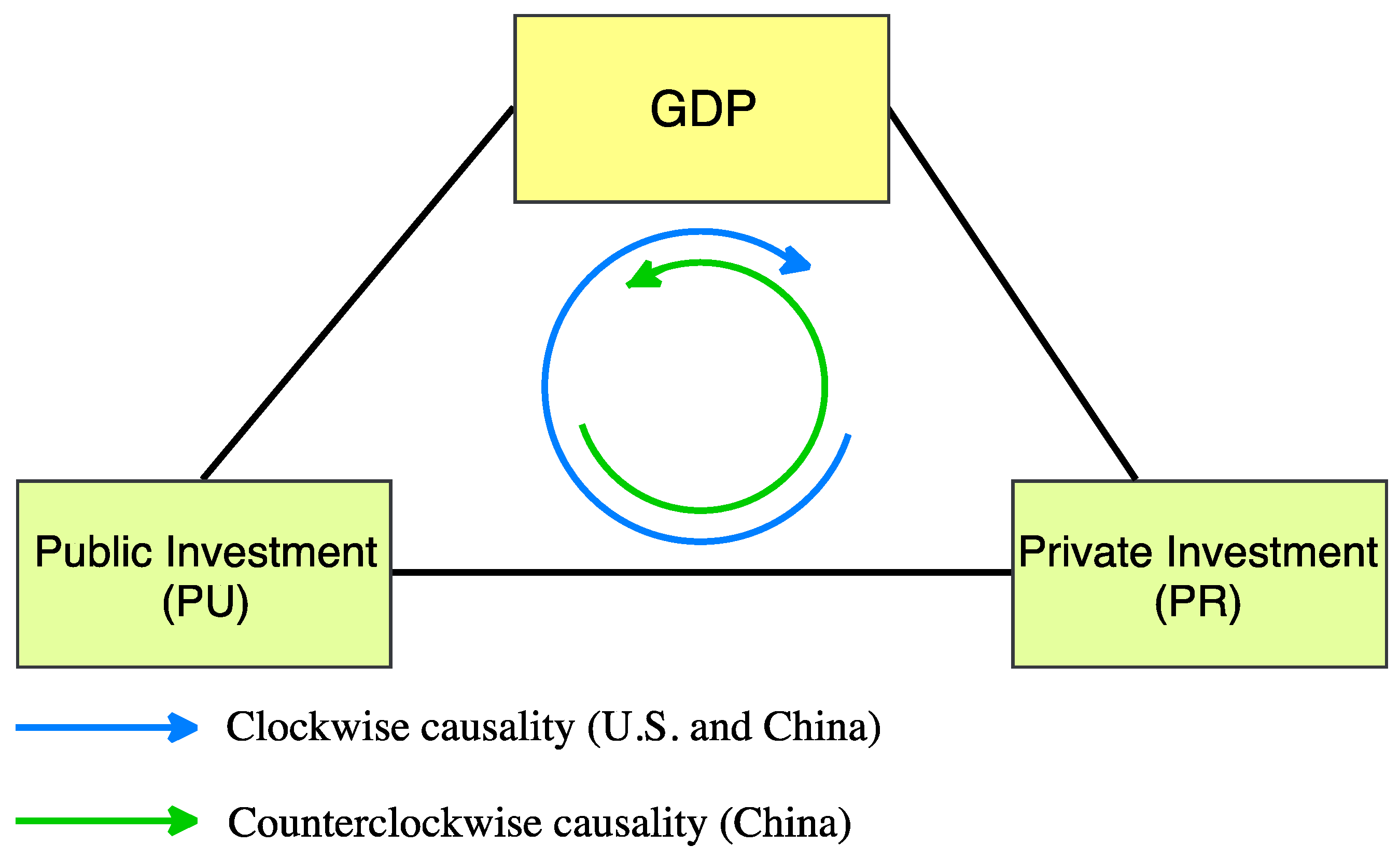
Figure 4 illustrates the strong and common causal relationship between the U.S. and China for sustainable economic growth among public and private investment and economic growth. The findings show that there is a feedback loop in either or both directions (i.e., clockwise or counterclockwise or both) of the causality chain through PU–GDP–PR–PU (see Figure 4). In the U.S., private investment promotes public investment, and this leads to economic growth. Last, economic growth feeds back to private investment. This chain forms a feedback loop in a clockwise direction between public and private investment through the GDP which sustains economic growth. On the other hand, China has the feedback loops in both directions for indirect transitions from public to private investment through the GDP and vice versa. This result implies that the existence of the feedback loop in Figure 4 is necessary for sustainable economic growth, which is a common behavior in the U.S. and China, but the direction of the loop can be determined by the socio-economic regimes of the countries. This assumption can be expanded to other countries with different levels of development and different political environments.

This study shows that the U.S. is a private-investment-driven economy in sustaining economic growth. Put differently, to sustain economic growth, decision-makers in the U.S. prioritize private sectors rather than public benefits, and design policies of public investment according to the needs of the private sector. This is because policymakers in a capitalist regime believe in the invisible hand, which is a core concept of mainstream economics, which describes the unintended social benefits of an individual’s self-interested actions. In other words, increasing private investment raises public investment automatically. Therefore, policymakers design public policies for the interests of the private sector to reach the benefits of the public in the big picture. This stimulates indirectly private investment by triggering economic growth. Furthermore, this strategy limits public investment by the requirements for private investment, thereby there is no crowding-out effect between them.

China, on the other hand, can be considered a more public-investment-driven economy in terms of sustainable economic growth, although there is a statistically weak feedback loop in the opposite direction, which is clockwise in Figure 4. In this regard, China’s government exerts a strong influence over the private sector by designing public policies for the benefit of the public rather than prioritizing the private sector. However, China realized the importance of the private sector after the 1990s to promote economic growth rapidly. Therefore, China has implemented new policies since the 1990s that enabled foreign direct investment in the economy and performed an unprecedented system that facilitated free enterprise and capitalist ideas within a socialist framework to flourish society along with the economy. Furthermore, China has empowered private sectors by aligning them with public policy and supported the public investment that resulted in the strong bidirectional and direct causal relationship between public and private investment. In other words, this indicates that these variables trigger each other without depending on economic growth.

Table 8. Overview of causality test results.

		Linear Causality	Nonlinear causality
China	Public => Private	***	***
	Private => Public	***	**
	Public => GDP	***	*
	GDP => Public	***	**
	Private => GDP	***	**
	GDP => Private	**	**
United States	Public => Private	✗	✗
	Private => Public	***	**
	Public => GDP	✗	**
	GDP => Public	***	✗
	Private => GDP	✗	✗
	GDP => Private	**	**

Notes: 1. ***, ** and * denote significance level at the 1%, 5% and 10%, respectively. 2. The X≠>Y denotes null hypothesis that indicates variable X does not Granger cause variable Y.

summarizes the findings from the linear and nonlinear causality between public and private investment and economic growth, and compares the overall results within and across the countries. China shows consistent bidirectional causalities in both linear and nonlinear settings for each pair of datasets, and the findings only differ at the significance level. These results provide strong evidence to support the bidirectional causalities in China between public and private investment and economic growth. The U.S. presents a common unidirectional causality running from private to public investment in both linear and nonlinear tests. Furthermore, there is no causality in both settings running from public to private investment. In the U.S., economic growth leads to private investment in both tests with an identical significance level. Moreover, the opposite direction, from private investment to the GDP, has no causality in both tests. Thus far, the study finds consistent results in both linear and nonlinear. However, there is a significant change in the direction of causality between linear and nonlinear tests for public investment and economic growth. In the linear causality, economic growth causes public investment but not vice versa. In the nonlinear causality, on the other hand, public investment leads to economic growth but not vice versa. This change in the nonlinear test provides evidence to reveal the common behavior for sustainable economic growth in the U.S. and China.

5. Conclusion

There are many studies in the literature investigating the linear macroeconomic relations based on public and private investment in cross-country and country-specific analyses by focusing on various perspectives and methodologies. However, there is a gap in the literature in exploring nonlinear causal relations among public-private investment and economic growth, particularly in the U.S. and China, in order to comparatively discuss policy implementations and potential implications. To narrow the gap, this study investigates nonlinear causal relationships between public-private investment and gross domestic product in the U.S. and China, which are the largest economies comprising about 40 percent of the global GDP in 2018 [8]. These countries show a similar pattern in economic growth and implementing sustainable development goals, although they follow considerably different socio-economic regimes and fall into different development levels (i.e., developed and developing countries). Therefore, there should be a common underlying mechanism in macroeconomic factors that fosters economic development. In this regard, the motivation behind the study is to reveal a common but hidden behavior of the nonlinear causal relations of given macroeconomic factors in these countries for sustainable economic growth.

This study contributes to the literature by providing robust evidence to propose a framework of sustainable economic growth for both developing and developed countries. First, there is a nonlinear causal relationship among the variables in this study between 1960 and 2015. Second, there exists a common feedback loop of causality in China and the U.S. for sustainable economic growth between public and private investment and the GDP. Third, the direction of the loop (i.e., clockwise or counterclockwise direction, or both) does not affect sustainable economic growth as long as such a causal loop exists between the variables. This direction is only dependent on the economic and social regimes of the countries but does not affect sustainable economic growth.

Thus far, we have investigated the interrelations among economic growth, public and private investment in the U.S. and China to provide evidence for sustainable economic growth. In what follows, we state several proposals for future research. First, we plan to comprehensively investigate the political systems (capitalistic vs. "market communism") and the cultural backgrounds of the U.S. and China on the economic growth effects. Second, we will expand this study to evaluate public-private-partnership business models, foreign direct investment (FDI), investment law, and the ease of doing business for the behavior of economic growth by analyzing the data from the literature, progress reports, and other sources (such as the United Nations, World Bank, and so on). Third, this study investigates the interrelations on aggregate public and private investment, thus we plan to examine the industry-specific data to evaluate if the findings are valid for specific industries. Next, there exist several directions towards follow-up research to explore different independent variables that might affect economic growth considerably, such as human development, education, and social welfare. These variables have the potential to increase labor productivity and flexibility to promote sustainable economic growth.

References

- Benhabib, J.; Spiegel, M.M. The role of human capital in economic development evidence from aggregate cross-country data. J. Monet. Econ. 1994, 34, 143–173. [Google Scholar] [CrossRef]
- Peet, R. Culture, imaginary, and rationality in regional economic development. Environ. Plan. A 2000, 32, 1215–1234. [Google Scholar] [CrossRef]
- Marrero, G.A.; Novales, A. Income taxes, public investment and welfare in a growing economy. J. Econ. Dyn. Control 2007, 31, 3348–3369. [Google Scholar] [CrossRef]
- Hindriks, J.; Peralta, S.; Weber, S. Competing in taxes and investment under fiscal equalization. J. Public Econ. 2008, 92, 2392–2402. [Google Scholar] [CrossRef] [Green Version]
- Waheed, A. Sustainability of public debt: Empirical analysis for Bahrain. J. Internet Bank. Commer. 2016, 21. [Google Scholar]
- Munnell, A.H. Policy Watch: Infrastructure Investment and Economic Growth. J. Econ. Perspect. 1992, 6, 189–198. [Google Scholar] [CrossRef]
- IMF Investment and Capital Stock Dataset, 1960–2015. Available online: https://www.imf.org/external/np/fad/publicinvestment/data/data122216.xlsx (accessed on 15 February 2019).
- IMF Gross Domestic Product (GDP). Available online: https://www.imf.org/external/datamapper/NGDPD@WEO/OEMDC/ADVEC/WEOWORLD (accessed on 1 October 2019).
- Buiter, W.H. “Crowding Out” and the effectiveness of fiscal policy. J. Public Econ. 1977, 7, 309–328. [Google Scholar] [CrossRef]
- Aschauer, D.A. Does public capital crowd out private capital? J. Monet. Econ. 1989, 24, 171–188. [Google Scholar] [CrossRef]
- Munnell, A.H. Why has productivity growth declined? Productivity and Public Investment. New Engl. Econ. Rev. 1990, 3–22. [Google Scholar]
- Greene, J.; Villanueva, D. Private Investment in Developing Countries: An Empirical Analysis. IMF Work. Pap. 1991, 38, 33–58. [Google Scholar] [CrossRef]
- Tatom, J.A. Public Capital and Private Sector Performance. Review 1991, 73. [Google Scholar] [CrossRef] [Green Version]
- Evans, P.; Karras, G. Are Government Activities Productive? Evidence from a Panel of U.S. Rev. Econ. Stat. 1994, 76, 1–11. [Google Scholar] [CrossRef]
- Erenburg, S.J. The Relationship Between Public and Private Investment; The Jerome Levy Economics Institute: Kansas City, MO, USA, 1993. [Google Scholar]
- Erenburg, S.J.; Wohar, M.E. Public and private investment: Are there causal linkages? J. Macroecon. 1995, 17, 1–30. [Google Scholar] [CrossRef]
- Voss, G.M. Public and private investment in the United States and Canada. Econ. Model. 2002, 19, 641–664. [Google Scholar] [CrossRef]
- Erden, L.; Holcombe, R.G. The effects of public investment on private investment in developing economies. Public Financ. Rev. 2005, 33, 575–602. [Google Scholar] [CrossRef]
- Mittnik, S.; Neumann, T. Dynamic effects of public investment: Vector autoregressive evidence from six industrialized countries. Empir. Econ. 2001, 26, 429–446. [Google Scholar] [CrossRef]
- Barro, R.J. Government spending in a simple model of endogeneous growth. J. Polit. Econ. 1990, 98, 103–125. [Google Scholar] [CrossRef] [Green Version]
- Xu, X.; Yan, Y. Does government investment crowd out private investment in China? J. Econ. Policy Reform 2014, 17, 1–12. [Google Scholar] [CrossRef] [Green Version]
- Dreger, C.; Reimers, H.E. Does public investment stimulate private investment? Evidence for the euro area. Econ. Model. 2016, 58, 154–158. [Google Scholar] [CrossRef]
- Bahal, G.; Raissi, M.; Tulin, V. Crowding-out or crowding-in? Public and private investment in India. World Dev. 2018, 109, 323–333. [Google Scholar] [CrossRef]
- Ari, I.; Akkas, E.; Asutay, M.; Koç, M. Public and private investment in the hydrocarbon-based rentier economies: A case study for the GCC countries. Resour. Policy 2019, 62, 165–175. [Google Scholar] [CrossRef]
- Afonso, A.; St. Aubyn, M. Economic growth, public, and private investment returns in 17 OECD economies. Port. Econ. J. 2019, 18, 47–65. [Google Scholar] [CrossRef] [Green Version]
- Deleidi, M.; Iafrate, F.; Levrero, E.S. Public investment fiscal multipliers: An empirical assessment for European countries. Struct. Chang. Econ. Dyn. 2020, 52, 354–365. [Google Scholar] [CrossRef]
- Masten, I.; Grdović Gnip, A. Macroeconomic effects of public investment in South-East Europe. J. Policy Model. 2019, 41, 1179–1194. [Google Scholar] [CrossRef]
- Abdul, A.; Furceri, D.; Topalova, P. The macroeconomic effects of public investment: Evidence from advanced economies. J. Macroecon. 2016, 50, 224–240. [Google Scholar]
- Ari, I.; Koc, M. Sustainable financing for sustainable development: Understanding the interrelations between public investment and sovereign debt. Sustainability 2018, 10, 3901. [Google Scholar] [CrossRef] [Green Version]
- Ari, I.; Koc, M. Sustainable Financing for Sustainable Development: Agent-Based Modeling of Alternative Financing Models for Clean Energy Investments. Sustainability 2019, 11, 1967. [Google Scholar] [CrossRef] [Green Version]
- IMF FAD Investment and Capital Stock Database 2017: Estimating Public, Private, and PPP Capital Stocks; International Monetary Fund: Washington, DC, USA, 2017.
- IMF Estimating the Stock of Public Capital in 170 Countries; IMF Fiscal Affairs Department (FAD): Washington, DC, USA, 2017.
- Dickey, D.A.; Fuller, W.A. Likelihood Ratio Statistics for Autoregressive Time Series with a Unit Root. Econometrica 1981, 49, 1057–1072. [Google Scholar] [CrossRef]
- Zivot, E.; Andrews, D.W.K. Further evidence on the Great Crash, the oil price shock, and the unit root hypothesis. J. Bus. Econ. Stat. 1992, 10, 251–270. [Google Scholar]
- Granger, C.W.J. Investigating causal relations by econometric models and cross-spectral methods. Econometrica 1969, 37, 424–438. [Google Scholar] [CrossRef]
- Johansen, S. Testing weak exogeneity and the order of cointegration in UK money demand data. J. Policy Model. 1992, 14, 313–334. [Google Scholar] [CrossRef]
- Brock, W.A.; Dechert, W.D.; Scheinkman, J.A. A Test for Independence Based on the Correlation Dimension; Econometric reviews: Madison, WI, USA, 1987. [Google Scholar]
- Toda, H.Y.; Phillips, P.C.B. Vector autoregressions and causality: A theoretical overview and simulation study. Econom. Rev. 1994, 13, 37–41. [Google Scholar] [CrossRef]
- Toda, H.Y.; Yamamoto, T. Statistical inference in vector autoregressions with possibly integrated processes. J. Econom. 1995, 66, 225–250. [Google Scholar] [CrossRef]
- Schwarz, G. Estimating the dimension of a model. Ann. Stat. 1978, 6, 461–464. [Google Scholar] [CrossRef]
- Grassberger, P.; Procaccia, I. Measuring the strangeness attractors. Phys. D 1982, 170–189. [Google Scholar]
- Chiou-Wei, S.Z.; Chen, C.-F.; Zhu, Z. Economic growth and energy consumption revisited—Evidence from linear and nonlinear Granger causality. Energy Econ. 2008, 30, 3063–3076. [Google Scholar] [CrossRef]
- Brock, W.A.; Scheinkman, J.A.; Dechert, W.D.; LeBaron, B. A test for independence based on the correlation dimension. Econom. Rev. 1996, 15, 197–235. [Google Scholar] [CrossRef]
- Baek, E.; Brock, W. A general test for nonlinear Granger causality: Bivariate model. In Iowa State University and University of Wisconsin at Madison Working Paper; Iowa State University: Ames, IA, USA; University of Wisconsin at Madison: Madison, WI, USA, 1992. [Google Scholar]
- Hiemstra, C.; Jones, J.D.J. Testing for linear and nonlinear Granger Causality in the stock price- volume relation. J. Finance 1994, 49, 1639–1664. [Google Scholar]
- Diks, C.; Panchenko, V. A new statistic and practical guidelines for nonparametric Granger causality testing. J. Econ. Dyn. Control 2006, 30, 1647–1669. [Google Scholar] [CrossRef] [Green Version]
- Engle, R.F.; Granger, C.W.J. Co-Integration and Error Correction: Representation, Estimation, and Testing. Econometrica 1987, 55, 251–276. [Google Scholar] [CrossRef]
- Johansen, S.; Juselius, K. Maximum likelihood estimation and inference on cointegration—With applications to the demand for money. Oxf. Bull. Econ. Stat. 1990, 52, 169–210. [Google Scholar] [CrossRef]
- Mawejje, J.; Sebudde, R.K. Tax revenue potential and effort: Worldwide estimates using a new dataset. Econ. Anal. Policy 2019, 63, 119–129. [Google Scholar] [CrossRef]
- Fisher, W.H.; Turnovsky, S.J. Public investment, congestion, and private capital accumulation. Econ. J. 1998, 108, 399–413. [Google Scholar] [CrossRef]
- Vijverberg, W.P.M.; Vijverberg, C.-P.C.; Gamble, J.L. Public capital and private productivity. Rev. Econ. Stat. 1997, 79, 267–278. [Google Scholar] [CrossRef]
Figure 1.
Public and private investment in (a) China and (b) the U.S. [7].
Figure 2.
The GDP of the U.S. and China [8].
Figure 3.
The causality framework.
Figure 4.
The common causality relationship between developing (China) and developed (the U.S.) countries for sustainable economic growth.