The Impact of Air Pollution on Domestic Tourism in China: A Spatial Econometric Analysis


School of Business Administration, Southwestern University of Finance and Economics, Chengdu 611130, China
*
Author to whom correspondence should be addressed.
Sustainability 2019, 11(15), 4148; https://doi.org/10.3390/su11154148
Submission received: 23 June 2019
/
Revised: 27 July 2019
/
Accepted: 30 July 2019
/
Published: 1 August 2019
(This article belongs to the Special Issue Tourism Sustainability in Developing Countries and Emerging Economies)
Abstract
:This study utilizes a spatial econometric model to analyze the impact of air pollution on domestic tourism in China. Based on a panel dataset covering 337 cities from 2004–2013, this study derives the following findings. (1) Air pollution significantly reduces domestic tourist arrivals in the local city. On average, if the concentration of PM (particulate matter equal to or less than 2.5 micrometers in width) in one city increases by 1 g/m, the number of domestic tourists to the city declines by 0.7%. (2) Air pollution demonstrates significant spatial spillover effects. If the PM in other cities simultaneously increases by 1 g/m, the number of domestic tourists traveling to the local city rises by 4.1%. (3) The magnitude of the spillover effects of air pollution is larger than the negative direct effects on local cities. This study suggests that enhancing air quality in the local area will effectively promote the domestic tourism industry in the local city. In addition, it is implied that a simultaneous improvement in the air quality in all cities might not lead to an increase in the number of domestic tourist arrivals. Thus, in order to deal with the spillover effects of air pollution on the domestic tourism industry, local governments should make efforts to develop cross-city or cross-region tourism.
1. Introduction
Given that air pollution poses a great threat to human health, the climate, and ecosystem, in 2014, the United Nations Environment Assembly (UNEA) made air quality improvement a top priority for world sustainable development [1]. Air pollution also puts enormous stress on sustainable growth in tourist arrivals and receipts. Previous studies have reported the impact of air pollution on the tourism industry worldwide, from both micro [2,3,4,5] and macro perspectives [6,7]. In recent years, China’s tourism industry has seen unprecedented development and become one of the world’s top inbound and outbound tourist markets [8]. However, the severe air pollution problem in some Chinese districts has harmed tourism development. For instance, in 2016, it was reported that hundreds of flights were canceled in Beijing because thick smog cut visibility to less than 200 m [9]. Given that air pollution in China has bought disruption to outdoor travel activities due to low visibility and increased health risk, the extensive air pollution problem in China has received a lot of attention from scholars in the tourism industry. However, studies focus mainly on the impact of air pollution on inbound tourism [2,3,4,5], and few research efforts have been dedicated to the impact of air pollution on China’s domestic tourism market, with the exceptions of Liu et al. [10], Peng and Xiao [11], and Zhang et al. [12].
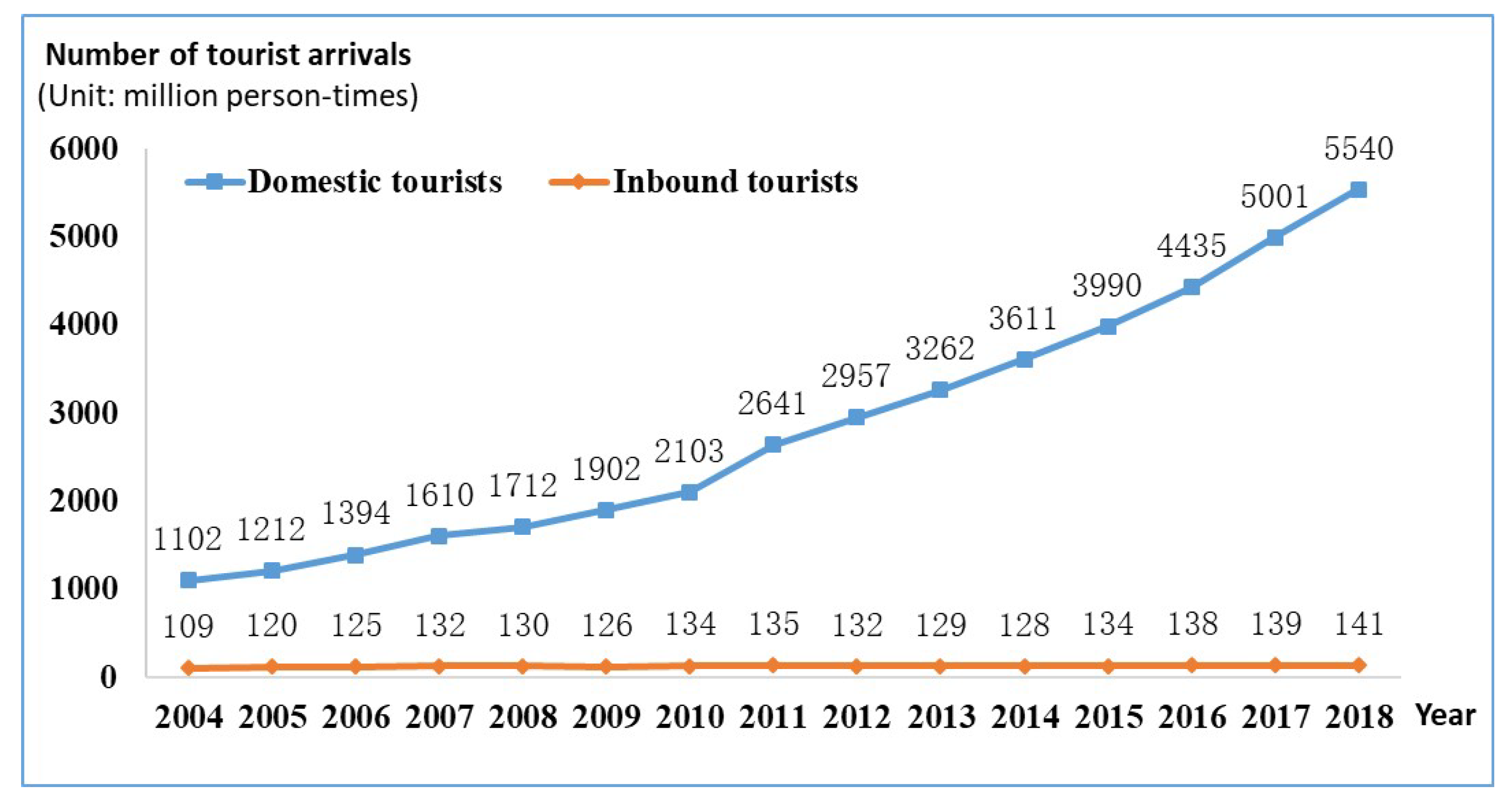
It is widely acknowledged that China has become one of the world’s most important tourism destinations, with 141 million inbound visits in 2018 [13]. However, the rise of China’s domestic tourism market is also worthy of attention, as the number of domestic tourist trips reached 5.54 billion person-times in 2018, with an annual increase of 10.8%. Figure 1 shows the number of domestic and inbound tourist arrivals in China during the period 2004–2018. It is apparent that while the scale of China’s domestic tourism market is much larger, its growth is also faster than inbound tourism. Therefore, it is important to have a good understanding of China’s domestic tourism industry.
Air quality influences domestic travel [10,11,12]. It is worth mentioning that poor air quality in China has given rise to the widespread popularity of smog avoidance travel packages [14]. Ctrip, a leading online travel agent (OTA) in China, reported that travelers tend to search keywords such as “smog escape”, “lung cleaning”, and “forests” in order to find a destination with fresh air. The top ten “haze evading” cities are Beijing, Tianjin, Shanghai, Chengdu, Guangzhou, Shenzhen, Chongqing, Xi’an, Wuhan, and Jinan. The top domestic destinations to escape smog include, but are not limited to, the following districts: Sanya, Harbin, Kunming, Xiamen, Jiuzhaigou, Zhangjiajie, Beihai, and Lijiang [15]. There are a number of OTAs that have released smog-escape travel products. Furthermore, it is reported that the rise of rural tourism in China contributes to an increase in domestic tourism. Rural tourism in China usually features fresh air and tranquil pastoral scenery. The Chinese Tourism Academy estimated that Chinese tourists spent around $200 billion on rural tourism in 2017 [16], implying that seeking fresh air and unspoiled nature has become a pull factor that motivates the Chinese to travel domestically. According to Yang and Fik [17], the unintended side effects caused by a region’s characteristics (e.g., transport infrastructure, tourism resources) on tourism in neighboring regions is referred to as spillover effects. However, few studies have examined the spillover effects of air pollution on domestic tourism in China. To address the aforementioned gaps, this study aims to investigate how and to what extent air pollution influences China’s domestic tourism industry by taking spatial interactions among different districts into account.
Based on a panel dataset of 337 Chinese cities for the period 2004–2013, this study utilized a spatial econometric model to evaluate the impact of air pollution on China’s domestic tourism. Importantly, this study examines the spillover effects on tourism flows among different cities. This study is expected to help Chinese policy makers understand the consequences of air pollution on the domestic tourism industry. Furthermore, the results could help destination marketers assess how to position travel products to meet domestic travelers’ needs.
This study contributes to the academic literature in several aspects. First, this study empirically evaluates the impact of air pollution on China’s domestic tourism based on a wide sample of cities, which supplements the findings of the existing literature on the impact of air pollution on China’s international tourism industry, or based on using Beijing as a case study. Second, by utilizing a spatial econometric framework, this study is among the first to assess the unintended side effects of air pollution from other cities on local cities’ domestic tourism industry. The results of this study are expected to help local governments and tourism organizations develop strategies to reach a sustainable balance between the domestic tourism industry and environmental quality management.
2. Literature Review
This study is closely relevant to three streams of literature. The first stream studies the impacts of air pollution on tourism. The second stream evaluates tourism spatial spillover effects. The third concerns the spatial spillover impacts of air pollution in China.
2.1. Impacts of Air Pollution on Tourism
A number of studies have found a negative impact of air pollution on tourism, which supports the assertion by Buckley [18] that the tourism industry remains far from sustainable. For instance, Anaman and Looi [6] estimated the effect of haze-related air pollution on the inbound tourism industry in Brunei Darussalam. According to their estimate, the haze-related air pollution reduced monthly arrivals by about 28.7%, resulting in total direct loss of about eight million Brunei dollars (BND). Sajjad et al. [7] regarded deforestation and natural source depletion as two negative indicators of tourism development and revealed that, on average, air pollution in Asia and Africa negatively influenced the tourism industry. Some scholars have broadened the scope of research by focusing on the impact of adverse climate changes, which may exacerbate air pollution problems. Hamilton et al. [19] indicated that the growth of international tourism is projected to decrease in the long term due to climate change. Gössling et al. [20] indicated that the climate change of destinations is important in forming travel decisions. Based on an overview of the relationship between tourism and global climate change, Pang et al. [21] suggested that climate change could negatively influence the tourism industry by making trip planning difficult and decreasing visitor satisfaction.
In recent years, some areas of China have suffered from serious air pollution. This phenomenon has gained attention from scholars who seek to investigate the impact of particle pollution on China’s tourism industry. Given that Beijing is China’s capital city and one of the top tourism destinations, its air pollution is especially remarkable. A number of studies took Beijing as a case study and examined the impact of air pollution on the tourism industry from a micro-level perspective. Li et al. [22] found that smog concern among international travelers in Beijing would negatively influence their satisfaction. Zhang et al. [12] indicated that tourists who intend to visit Beijing in the next two years saw haze pollution as a crucial influencing factor when making decisions. Peng and Xiao [11] later examined domestic travelers’ attitudes towards smog in Beijing, indicating that travelers’ perceived health risk and experience risk associated with smog had a negative impact on destination image and subsequently led to a behavioral tendency of avoidance.
Besides Beijing, Cheung and Law [3] examined the inbound tourists’ perceptions of choosing Hong Kong as a tourist destination. It was found that Asian visitors were more concerned with air quality when selecting a destination than Western travelers. Law and Cheung [4] further indicated that international travelers generally did not regard air pollution as a concern while making travel decisions, but they became aware of Hong Kong’s air quality issues after their visits. At a national level, Becken et al. [2] reported that the U.S. and Australian residents regarded air pollution issues in China as one of the major travel risks, which negatively influenced destination image and visit intention to China. Based on a cross-sectional sample survey, Qiao et al. [5] reported that for Australian residents, the pollution and air quality issues in China were considered as the substantially negative factors when considering travel to China.
From a macro perspective, the negative impact of air pollution on China’s inbound tourism industry has been verified by previous studies. In the case of Beijing, Tang et al. [23] applied monthly times series data from January 2004–December 2015 and found air pollution had a negative impact on inbound tourism in the long term rather than the short term. Deng et al. [24] utilized panel data on 31 Chinese provinces and found that industrial waste gas emissions had a significant negative effect. Dong et al. [25] analyzed the data from 274 Chinese cities during the period 2009–2012, confirming the negative impact of air pollution on inbound tourism in China. Liu et al. [10] used panel data from the 17 undeveloped provinces of China during the period 2005–2015 and found that domestic travelers in China were more sensitive to PM concentration than international travelers. Wang et al. [26] provided further evidence of the impact of air pollution on outbound tourism in China. Using data from a dominant online travel agent (OTA) in China, they discovered that air pollution is a push factor that motivates Chinese people to travel abroad.
The literature on the impact of air quality in the place of destination on the tourism industry substantially outnumbered the studies on the impact of air quality in the place of origin. In addition, prior studies tended to place much greater emphasis on inbound tourism, neglecting the domestic tourism market in China. This current study intends to shrink the gap in the literature by focusing on domestic tourism in China and using a spatial analysis method to investigate the impacts of air pollution in both tourist origin and destination cities.
2.2. Spatial Spillover Effects in the Tourism Industry
Previous studies have confirmed the existence of spillover effects in the tourism industry. From the supply side, Li et al. [27] examined the role of tourism development in reducing regional income inequality in China using a spatiotemporal autoregressive model, indicating that the development of domestic tourism significantly narrows regional inequality. Ma et al. [28] showed the spatial spillover effect of tourism development on urban economic growth. Previous studies also have identified a spatial correlation between tourism building investments and tourist revenues, the flow of tourist capital and labor and tourism-related economic growth, as well as local tourism development patterns (e.g., hotel infrastructure, tourism resource endowments) and regional tourism growth [17,29]. It has also been found that the growth of cruise tourism has a spillover effect on other tourism sectors, such as hotels and restaurants [30].
From the demand side, previous studies examined the spatial spillover effects in tourism flows. Yang and Wong [31] found spatial spillover effects in both inbound and domestic tourism flows to 341 cities in mainland China. It is suggested that physical infrastructure factors, tourist attractions, and the severe acute respiratory syndrome (SARS) outbreak exhibited spatial spillover effects. Investigating 55 countries participating in the “One Belt, One Road” initiative, Deng and Hu [32] confirmed the existence of positive spillover effect in Chinese outbound tourist flows among countries with geographic and cultural proximity. Using data from 98 cities in Eastern China during the period 2004–2012, Zhou et al. [33] also found that tourist attractions in the regions surrounding a specific destination had a positive spatial spillover effect on tourist flows to that destination.
2.3. Spatial Spillover Effects of Air Pollution in China
The existing literature includes spatial analyses of urban air pollution and air pollution control. Based on a panel covering 285 cities, Feng et al. [34] utilized the spatial Durbin model to examine the spatial spillover effect of air pollution control on urban development quality in China, providing evidence of heterogeneity within different spatial regions in China. Fang et al. [35] later discovered the unintended spillover effects of regional air pollution policies on mitigating air pollution in urban areas. Previous research has also explored the spatial spillover effect of air pollution on public health and healthcare expenditure in China [36,37].
Based on the above review of the literature on the impact of air pollution and spatial spillover effects, it can be concluded that the spatial correlation between air pollution and tourist flows is underexplored. A notable exception is the research of Deng et al. [24], who reported that air pollution had a negative spatial spillover effect on China’s inbound tourism industry, implying that international tourists are unlikely to visit a province that is surrounded by seriously polluted regions. Similarly, this finding was later supported by Xu et al. [38], who conducted a spatial analysis on inbound tourism in 174 cities of mid-eastern China. It seems that no empirical studies have examined the spatial spillover effects of air pollution on the domestic tourism industry. This current study attempts to shrink this gap in the literature.
On the basis of the literature, two hypotheses are proposed to address precisely whether and to what extent air pollution influences the sustainable development of the domestic tourism industry.
Hypothesis 1.
Air pollution in the local city negatively affects the number of domestic tourist arrivals in that city.
Hypothesis 2.
Air pollution in other cities positively affects the number of domestic tourist arrivals in the local city.
3. Empirical Model and Data
3.1. Regression Model
The spatial Durbin model (SDM) is widely used in spatial analysis of tourism economics, because it considers both the spatial lagged dependent and independent variables [24,39]. We use the SDM as follows:
where the dependent variable y refers to , the logarithmic value of the number of domestic tourist arrivals (in 10,000 person-times) in a city during one year. The vector is a set of explanatory variables. The core explanatory variable of interest is , the concentration density (g/m) of particulate matter in the air that is 2.5 micrometers or less in width. Besides, we also considered six important control variables: , , , , , and . (i) is an index for the abundance of tourism resource endowment, calculated by the number of 5A- and 4A-rated scenic spots. One 5A spot is regarded as equal to two 4A spots, as a 5A spot is usually considered to be much more attractive than a 4A spot. (ii) is an indicator of tourism infrastructure availability. As hotels are one of the most important tourism facilities, we used the number of star-rated hotels divided by the local population to index this variable. (iii) is an indicator of the density of transportation infrastructure, proxied by the road length (km) per area (km). (iv) refers to government size, measured by the ratio of fiscal spending to local GDP. This variable intends to capture the role of local government in tourism development. (v) is the logarithmic value of the gross domestic product (GDP) per capita. This variable measures the degree of economic development. (vi) is the logarithmic population within the city. The population is included as a control variable to control for the possible economies of scale in the tourism industry.
is a spatial weight matrix. In our model, is a distance matrix constructed based on the longitude and latitude data of the cities. Based on the classical assumption that spillover effects decline as the geographic distance increases, the off-diagonal elements of were set equal to the inverse of the linear distance (km) between two cities, and the diagonal elements were zero. Another spatial weight matrix will be used for the robustness check, which will be discussed in detail in Section 4.3.
u refers to the fixed effect (FE) or random effect (RE) incorporated into the panel data model, depending on whether we apply an FE or RE model. is the error term. , , and are coefficients to be estimated. Based on these coefficients, we were able to measure the direct and indirect effects of each explanatory variable. We focus in particular on the effects of air pollution.
3.2. Data
The data were collected from several different sources. The data of PM were taken from NASA’s Global Annual PM Grids data [40,41]. Data of , , , , , and came from the China Statistical Yearbook for Regional Economy [42]. The data regarding were collected from the public information released by the local governmental departments of tourism in different provinces. The spatial weight matrix is a distance matrix constructed based on the longitude and latitude data from the National Geomatics Center of China (NGCC).
The dataset comprised both temporal and spatial dimensions. In terms of its time dimension, it covered the period from 2004–2013. In fact, the China Statistical Yearbook for Regional Economy provides data for the period 2002–2013. The data for 2002 and 2003 were intentionally dropped because the tourism industry in China was greatly affected by the SARS issue in 2003 [43]. Thus, the data before and after 2003 are not comparable. The sampling period ended in 2013, because the city-level tourism data were substantially incomplete since 2014. In terms of its spatial dimension, it had a wide geographic range covering almost all areas within Mainland China. To be precise, the sample consisted of 337 districts in Mainland China, covering all four province-level municipalities (Beijing, Shanghai, Tianjin, and Chongqing) and all prefecture-level administrative regions except Sansha City of Hainan Province. For convenience, these administrative districts are denoted as “cities” in the rest of the paper. Sansha City, which was established in 2012, was excluded due to its extremely small population size of approximately 3000 residents and a lack of relevant statistical data. Chaohu City in Anhui Province lacked data during 2011–2013, because it was no longer a prefecture-level city due to the adjustment of administrative division in 2011. Thus, for simplicity, the missing values during the period 2011–2013 were imputed using the data for 2010. After a data cleansing process, a balanced panel dataset of 337 cities for 10 years was kept for further analyses, which generated 3370 observations. The summary statistics of the variables used in our regressions are shown in Table 1. (The data are available online as supplementary materials).
4. Results
The empirical results are presented in this section. We first show the results of the statistical tests of spatial autocorrelation. Then, we demonstrate the main estimation results for the regression model expressed by Equation (1). After that, several robustness checks are discussed. Some important extended analyses based on the estimates are presented at the end of this section.
4.1. Statistical Tests of Spatial Autocorrelation
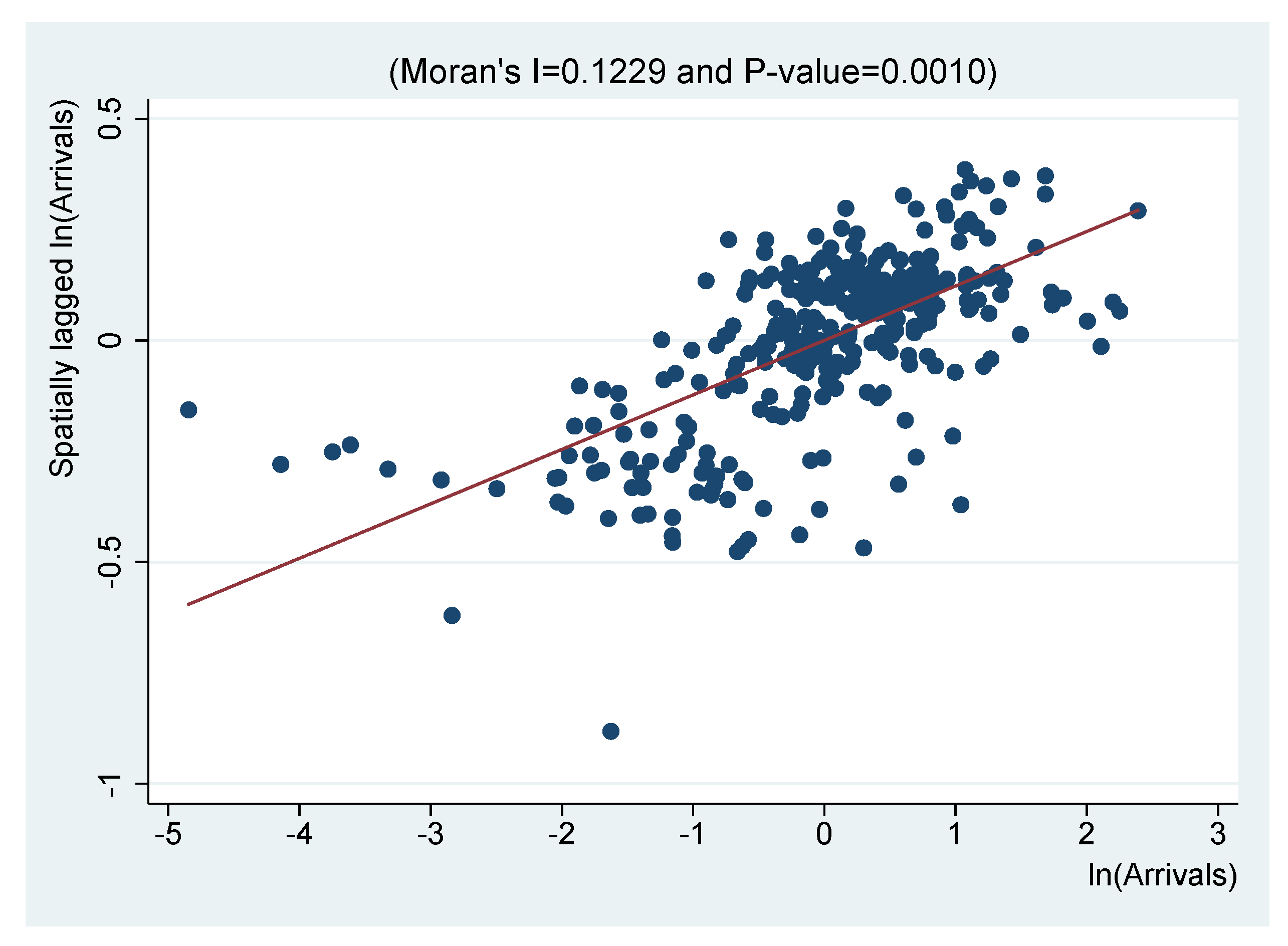
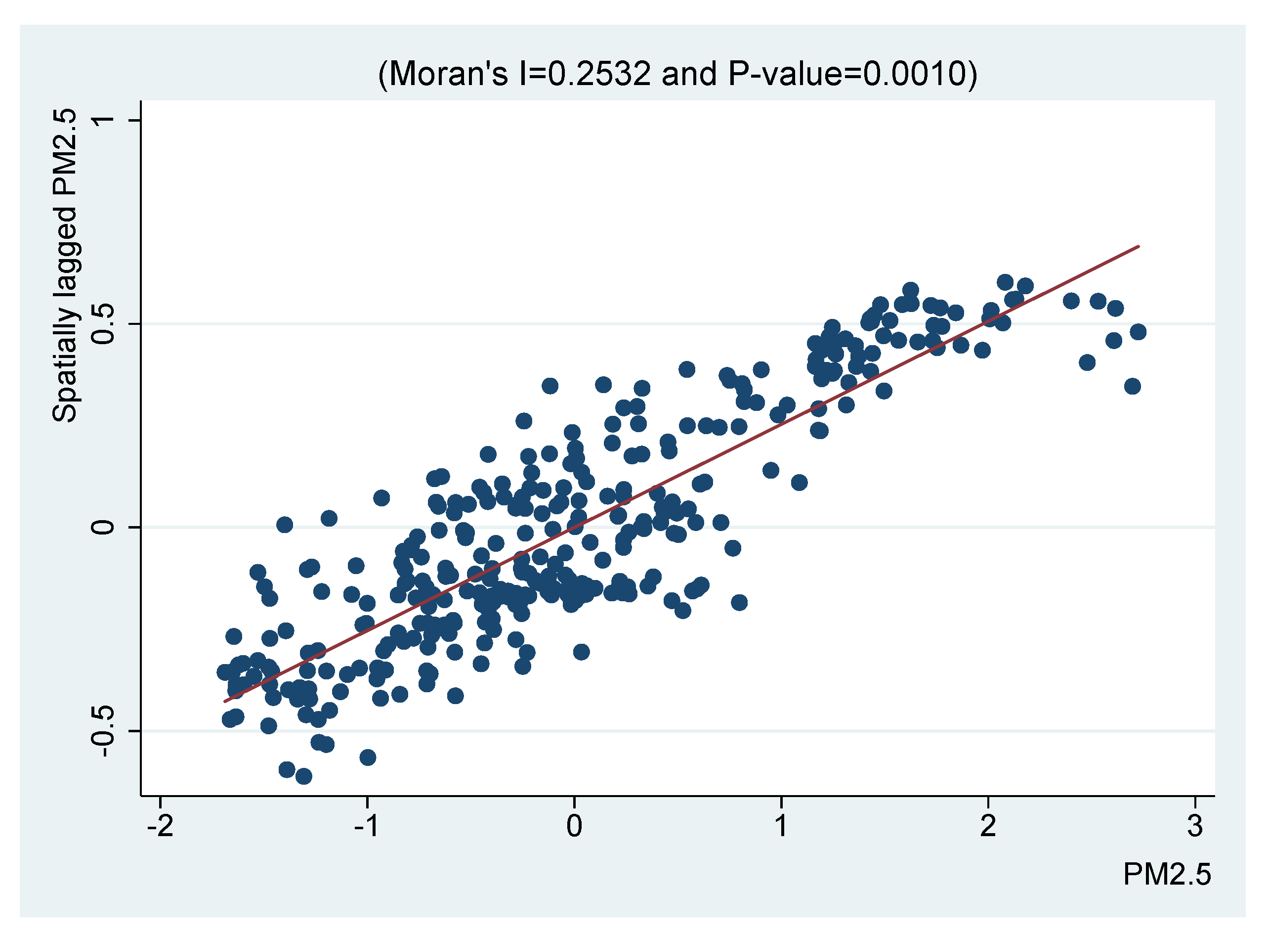
Table 2 shows the estimated value of Moran’s I, a well-known measure of spatial autocorrelation, and the associated z-score for the variables of and in each sample year. As presented in the table, tourism and air pollution both displayed statistically-significant spatial autocorrelation.
Next, scatter plots were used to visualize the existence of spatial autocorrelation of and , shown in Figure 2 and Figure 3, respectively. We only present the scenario for 2013 for the sake of simplicity. Scenarios in other years yielded similar results. Figure 2 and Figure 3 respectively exhibit strong signs of spatial autocorrelation of the domestic tourism industry and air pollution data. In other words, the distributions of tourist arrivals and PM were not geographically random, but demonstrated substantial spatial agglomeration in space. Therefore, this study adopted a spatial econometric model to take into account the spatial spillover effects among independent and dependent variables.
4.2. Main Estimation Results
The main estimation results for Equation (1) are reported in this subsection. Before running regressions, we first used the Hausman test to decide whether we should apply an FE model or RE model. The result of the Hausman test indicated that the FE model was preferred. Thus, we used the FE model to estimate Equation (1) and report the estimated coefficients in Column (a) of Table 3. The coefficient of was −0.007 and was statistically significant at the 1% level, indicating that air pollution within a local city reduced domestic tourist arrivals in the city (It is notable that within a framework of SDM, in order to measure the “direct effect” of air pollution on local tourism, we must consider the complex spatial feedbacks among different variables across the sample cities. Hence, at this moment, we do not discuss the implied direct effect of air pollution and the associated economic significance of the estimated coefficients in Table 3. The relevant discussion is postponed until Section 4.4.2.). In addition, the coefficient of was 0.033 and was significant at the 1% level, which confirmed the existence of spatial spillover effects of air pollution on the domestic tourism industry across different cities. It is important to note that the coefficient was positive, indicating that air pollution in other cities in fact tended to increase the number of tourists traveling to the local city.
In terms of control variables, hotel density (), government size (), GDP per capita (), and population scale () all had a statistically-significant positive impact on domestic tourist arrivals. The number of scenic spots () and road density () did not generate significant effects. Regarding the spatial spillover effect of control variables, it can be seen from the table that the number of scenic spots in other cities () and transportation infrastructure density in other cities () had a significantly negative impact. These support the viewpoint of the existence of strong competition in the domestic tourism industry among different cities: the improvement of tourism resources and transportation infrastructure in other regions reduced a local city’s attractiveness to domestic tourists. The government size in other cities () had a significantly positive coefficient, perhaps because there were some cooperative activities among the local governments across different cities to promote tourism. The population size in other cities () showed a significant negative coefficient, suggesting that large cities might depress the tourism attractiveness of small cities. The availability of hotel () and GDP per capita () failed to yield significant spatial spillovers.
4.3. Robustness Checks
We conduct several robustness checks for our main estimation results and report the estimated coefficients in Columns (b), (c), and (d) of Table 3.
We first considered the issue of model misspecification. Although the Hausman test supports the usage of the FE model, it is still beneficial to test whether our estimation results were sensitive to an alternative model specification. We re-estimated Equation (1) using the RE model and report its results in Column (b) of Table 3. A comparison between Columns (a) and (b) shows that the difference between FE and RE estimates was small.
Next, we considered whether the regression was robust if we used an alternative index of air pollution. In the model shown in Column (a), the core explanatory variable was the density of PM (g/m), which is a straightforward measure of air pollution. However, it is possible that the severity of PM pollution is not linearly correlated with the physical density of PM in the air. For example, an increase of PM concentration from 50 g/m–100 g/m may have a substantially distinct influence compared to an increase from 150 g/m–200 g/m. Considering this, we made a nonlinear monotonic transformation by converting the PM density value to the corresponding air quality index (AQI) value, according to the Technical Regulation on Ambient Air Quality Index (HJ 633-2012) published by China’s Ministry of Environmental Protection. This technical regulation provides a reliable guide to the nonlinear relationship between the original density data of air pollutant(s) and the AQI. We used the calculated AQI to replace in Equation (1) and report the regression results in Column (c) of Table 3. The results supported our previous findings.
As the estimates in the spatial econometric model depended on the setup of a spatial weight matrix, we should investigate whether our previous results were robust if we utilized another weight matrix. Previously, we set the spatial distance matrix with off-diagonal elements equal to the inverse of the distance between two cities. Now, we exploited another matrix : the diagonal element was zero, and the off-diagonal element was one if the distance between city i and j was below or equal to 800 km, and zero otherwise. We regarded 800 km as a proper threshold value because many domestic tourists travel by car, bus, and train with an average speed of around 100 km/h. At this speed, traveling for 800 km takes 8 h, equivalent to the length of working hours on a typical working day. Thus, a distance below and above 800 km can be reasonably regarded as “near” and “far”, respectively. (We also tried other values, such as 500 km or 1000 km, as a threshold to construct the binary matrix , and found similar regression results. To save space, we only report the estimates based on the weighting matrix using 800 km as the threshold.) Column (d) of Table 3 shows our estimates. It was found that the coefficient of was close to the previous estimates in the baseline model. The coefficient of became smaller, but was still positive and statistically significant at the 1% level.
In brief, the robustness checks validated the estimates based on the baseline model and confirmed our previous findings that air pollution damages domestic tourism in the local city, but tends to increase the domestic tourist arrivals in other cities.
4.4. Extended Analyses
We further analyzed our main estimation results presented in Section 4.2. We first examined the heterogeneity across different regions in China. Then, we decomposed the marginal effect of air pollution into two parts: direct effect and indirect effect.
4.4.1. Circumstances in Different Districts
As the eastern, central, and western areas of China are highly heterogeneous in the degree of economic and social development, it is possible that the impact of air pollution on domestic tourism is not homogenous over these three regions. To deal with this concern, we re-estimated Equation (1) for the subsamples of these three regions separately and then compared the results. The sample was divided according to the official classification by the National Bureau of Statistics of China. In our sample, 101, 105, and 131 cities belonged to the eastern, central, and western areas, respectively. Columns (a), (b), and (c) in Table 4 display the estimates for the eastern, central, and western subsamples, respectively. Focusing on the effect of air pollution, there were two main findings. (1) In all regions, air pollution generated a significant negative impact on domestic tourism in local cities. The significant negative coefficients of variable in Columns (a), (b), and (c) made this point clear. (2) In all regions, air pollution had a positive spatial spillover effect on domestic tourism in other cities. As displayed in the table, the coefficients of were positive in Columns (a), (b), and (c). In particular, the coefficients for the central and western regions were statistically significant at the 1% level.
Overall, the separate investigation on the three Chinese regions supported our previous argument based on Table 3. Our previous findings on the negative local effect and positive spillover effect of air pollution on domestic tourism were robust.
4.4.2. Decomposition of Direct and Indirect Effects
The marginal effect of the air pollution indicator can be decomposed into two components: “direct effect” and “indirect effect”. The former measures the average influence of air pollution in one city on the domestic tourism in the same city. The latter measures the average influence of air pollution in other cities on one city of reference (and equivalently, in a numerical sense, it measures the influence of air pollution in one city on other cities). The summation of the direct effect and indirect effect is referred to as “total effect”. This total effect can measure the aggregate impact of a simultaneous change with the same magnitude of air pollution in all regions. This implies that we can utilize the total effect to ascertain whether a coordinated air pollution control policy is feasible and beneficial.
It is notable that, although the estimates in Table 3 suggested the existence of a negative local effect and a positive spillover effect of air pollution on domestic tourism, the estimated coefficients of and in Equation (1) did not directly reflect the magnitude of the direct effect and indirect effect. Within a framework of SDM, in order to calculate the direct and indirect effects of air pollution on tourism, we must consider the complicated spatial feedbacks among different variables across the sample cities. Equation (1) is . This can be expressed as , where is the new residual term. Therefore, for the explanatory variable, the direct effect is measured by the mean value of the diagonal elements of matrix . Based on the same matrix, the indirect effect is measured by the mean value of the row sum of the non-diagonal elements. The summation of direct and indirect effects is the total effect of the corresponding variable. Our results are displayed in Table 5.
We first used the estimates on the baseline model in Table 3 to calculate the direct, indirect, and total effect. Row (a) of Table 5 gives the results. The coefficient of the direct effect was −0.007 with a statistical significance at the 1% level, indicating that a 1 g/m increase of PM concentration caused a decline of 0.7% in domestic tourist arrivals. In our sample, the mean value of tourist arrivals across all cities was 12.17 million person-times. Thus, a decline of 0.7% corresponds to a reduction of 85,190 person-times in domestic tourist arrivals. This was indeed a large loss. The coefficient of the indirect effect was 0.041 with statistical significance at the 5% level, indicating that the domestic tourists visiting the local city would rise by 4.1% if PM concentration in other cities simultaneously increased by 1 g/m. This was a substantial influence. According to our estimates, the size of the (positive) indirect effect exceeded the size of the (negative) direct effect. As a consequence, the total effect, equal to the direct effect plus the indirect effect, had a positive coefficient of 0.034. This positive value had an interesting implication: a simultaneous depravation in air quality in all cities actually increased the number of domestic tourists. This phenomenon might be explained by the possibility that air pollution stimulates the demand for tourism.
Next, we inspected the robustness of our estimates. In Row (b) of Table 5, we calculate the direct, indirect, and total effect of pollution based on the RE model in Table 3. The results were similar: a negative direct effect, positive indirect effect, and positive total effect. In Row (c) of Table 5, we report the calculation results using AQI as the independent variable. The results were close to those shown in Row (a). In Row (d) of Table 5, we estimated with the spatial weight matrix . The estimated direct effect was close to that in Row (a). The estimated indirect effect was still significantly positive, but had a magnitude considerably smaller than that in Row (a). The shrinkage in the size of indirect effect was because artificially imposed that the cities farther than 800 km had no effect. No matter the shrinkage of indirect effect, the magnitude of the estimated indirect effect was still larger than the direct effect, and the total effect was still positive.
In general, the baseline model and different robustness checks provided consistent results. Our core findings can be summarized as follows. (1) Air pollution had a significantly negative direct effect on the domestic tourist arrivals in the local city. This had an important policy implication: an improvement of air quality will effectively promote the development of domestic tourism in the local city. (2) According to our estimates, the magnitude of the positive indirect effect of air pollution in other cities was larger than the magnitude of the negative direct effect of air pollution in the local city. Thus, the total effect of air pollution was actually positive, which might be explained as a tourism-demand-inducement effect (i.e., the deterioration of environmental quality increases the demand of traveling to the regions with a relatively better environment).
5. Discussion and Implications
This study implies that air quality is an important consideration factor when domestic tourists select a travel destination. Hypothesis 1 was supported. The result is consistent with Cheung and Law [3], whose study indicated that Asian visitors are conscious of air quality when selecting a travel destination. This result is also in line with Peng and Xiao [11] who examined the impact of smog on the domestic travel demand for Beijing and found a significant impact of travel risk perception on avoidance tendency and Liu et al. [10] who used panel data from the 17 undeveloped provinces in China and reported that the number of domestic travelers is negatively correlated with PM concentration. This study supplements the literature based on a wide city-level sample. It is implied that air pollution is not only viewed as an international travel risk [2], but also poses a threat to domestic travel. Therefore, it is suggested that China should implement effective policies to reduce air pollution so as to ensure sustainable growth for its domestic tourism industry.
Additionally, this study suggests that air pollution in other cities in fact tends to increase the number of tourists traveling to the local city. Hypothesis 2 was supported. This kind of spatial spillover effect may be attributed to two reasons. To facilitate interpretation of this result, let us consider an area that consists of three cities: City A with good air quality and Cities B and C with air pollution problems. (1) The first reason is relevant to the increased tourism demand in air polluted areas. People dislike air pollution and are unwilling to stay in polluted places for a long time. The air pollution in Cities B and C may motivate the residents in those cities to travel, and of course, City A with relatively cleaner air will be an attractive destination. In this way, an increase in PM density in other cities causes a rise of tourist arrivals at the local city. This result supplements the finding by Wang et al. [26], who indicated that a deterioration of air quality in the place of origin increases outbound tourism demand. This study shows the possibility of the tourism-demand-inducement effect of air pollution on domestic tourism, which is consistent with previous findings indicating that seeking fresh air is a push motivational factor for travel, especially for wellness or rural tourism [44,45]. Thus, it is suggested that Chinese cities with fresh air or cities with better air quality than their neighboring cities could develop haze-avoidance tourism packages to attract customers who are eager to escape air pollution. (2) The second reason is relevant to the competition between local and other cities for domestic tourism. For instance, suppose that a resident in City B is planning to travel and there are two candidate destinations: Cities A and C. Naturally this potential tourist will compare the characteristics of these two cities. Holding all variables else constant, this tourist will prefer City A over C because of the difference in air quality. Following the same logic, the air pollution in City B will raise the relative attractiveness of City A to the tourists originating from City C, because poor air quality was found to influence travelers’ aesthetic judgments on destinations [46] and perceived health risk [11]. In this way, an increase in PM concentration in other cities diverts some potential tourists from those cities to the local city. An implication for tourism marketing is that online travel agents could add a filter function by PM to each destination so that customers could make better decisions when choosing a destination.
Finally, this study implies that a simultaneous improvement of air quality in all cities does not cause an increase in the number of domestic tourist arrivals in each city. In other words, in the short term, for the purpose of expanding domestic tourism, there is a non-cooperative game among different cities: while it is beneficial to control unilaterally for the air pollution in the local area, a joint activity to reduce pollution in all cities simultaneously is not preferred because the local city can actually benefit from the air pollution in other cities. However, from a long-term perspective, since a tourism destination might reach a “decline” phase (during which the visitor flows to the destination decrease) according to the tourism-life-cycle model [47], awareness about different regions’ joint tourism resources and cooperation opportunities could help rejuvenate a tourism destination. Moreover, given the damage of air pollution to human health, the Chinese government should still make efforts to remedy air quality problems for the foreseeable future. As such, in the long term, it is suggested that cross-region or cross-city tourism destinations should be developed to deal with the spillover effect of air pollution on domestic tourism.
6. Conclusions, Limitations, and Future Studies
Using a spatial Durbin model, this study empirically demonstrated the significant impact of air pollution on domestic tourism in China based on a wide sample covering 337 cities, for the period 2004–2013. The estimates indicated that local air pollution significantly harms domestic tourism in the local city, and the air pollution in other cities generates strong positive spillovers onto local domestic tourism. By decomposing the marginal effects of air pollution into the direct effect and indirect effect, it was found that the magnitude of the (positive) indirect effect was larger than the (negative) direct effect.
This study is subject to certain limitations. First, this study only used the number of domestic tourist arrivals as the dependent variable, because of the limitation of data availability. It could be promising to consider other tourism-relevant variables such as tourism receipts, tourists’ average expenditure, and length of stay. Second, this study was conducted using data from China, and it is still unknown whether the findings can be applied to other countries. It is suggested that future studies could assess the impact of air pollution on the domestic tourism industries in other countries, especially for those countries suffering severe pollution problems, such as India and Pakistan in Asia and several countries in Central and Eastern Europe. As revealed by this study, if different districts have dissimilar environmental quality, the cleanest district would have a substantial competition advantage in attracting domestic tourists. Third, the model did not take into account the impacts of other pollution sources and environmental factors, such as water pollution and forest coverage. Incorporating other environmental factors into the model could provide a more comprehensive understanding of the pollution–tourism nexus.
Supplementary Materials
The data used in the empirical analyses are available online at https://www.mdpi.com/2071-1050/11/15/4148/s1.
Author Contributions
Conceptualization and funding acquisition, D.D. and X.X.; methodology, data curation, formal analysis, and original draft preparation, D.D.; literature review and review and editing, X.X.; software, validation, and supervision, H.Y. and Y.Z.
Funding
This research was funded by the Fundamental Research Funds for the Central Universities (Grant Nos. JBK1801039 and JBK1809054).
Acknowledgments
The authors are grateful to the editors and four anonymous referees for their comments and suggestions.
Conflicts of Interest
The authors declare no conflict of interest.
References
- Melamed, M.L.; Schmale, J.; von Schneidemesser, E. Sustainable policy—Key considerations for air quality and climate change. Curr. Opin. Environ. Sustain. 2016, 23, 85–91. [Google Scholar] [CrossRef]
- Becken, S.; Jin, X.; Zhang, C.; Gao, J. Urban air pollution in China: Destination image and risk perceptions. J. Sustain. Tour. 2017, 25, 130–147. [Google Scholar] [CrossRef]
- Cheung, C.; Law, R. The impact of air quality on tourism: The case of Hong Kong. Pac. Tour. Rev. 2001, 5, 69–74. [Google Scholar]
- Law, R.; Cheung, C. Air Quality in Hong Kong: A Study of the Perception of International Visitors. J. Sustain. Tour. 2007, 15, 390–401. [Google Scholar] [CrossRef]
- Qiao, G.; Peng, S.; Prideaux, B.; Qiao, M. Identifying Causes for the Decline in International Arrivals to China-Perspective of Sustainable Inbound Tourism Development. Sustainability 2019, 11, 1723. [Google Scholar] [CrossRef]
- Anaman, K.A.; Looi, C.N. Economic Impact of Haze-Related Air Pollution on the Tourism Industry in Brunei Darussalam. Econ. Anal. Policy 2000, 30, 133–143. [Google Scholar] [CrossRef]
- Sajjad, F.; Noreen, U.; Zaman, K. Climate change and air pollution jointly creating nightmare for tourism industry. Environ. Sci. Pollut. Res. 2014, 21, 12403–12418. [Google Scholar] [CrossRef] [PubMed]
- Xinhua. China’s domestic, inbound tourist trips to top 5.1 bln this year. Xinhuanet, 20 December 2017. [Google Scholar]
- South China Morning Post. Hundreds of flights canceled in Beijing as thick smog lays siege to capital. South China Morning Post, 20 December 2016. [Google Scholar]
- Liu, J.; Pan, H.; Zheng, S. Tourism Development, Environment and Policies: Differences between Domestic and International Tourists. Sustainability 2019, 11, 1390. [Google Scholar] [CrossRef]
- Peng, J.; Xiao, H. How does smog influence domestic tourism in China? A case study of Beijing. Asia Pac. J. Tour. Res. 2018, 23, 1115–1128. [Google Scholar] [CrossRef]
- Zhang, A.; Zhong, L.; Xu, Y.; Wang, H.; Dang, L. Tourists’ Perception of Haze Pollution and the Potential Impacts on Travel: Reshaping the Features of Tourism Seasonality in Beijing, China. Sustainability 2015, 7, 2397–2414. [Google Scholar] [CrossRef]
- Xinhua. China’s inbound tourism remains steady in 2018. Xinhuanet, 5 February 2019. [Google Scholar]
- Arlt, W.G. As Smog Hits China, Chinese Tourists Seek Fresh Air on Pollution Free Holidays. Forbes, 5 January 2017. [Google Scholar]
- China Daily. Top 8 domestic destinations to escape smog. China Daily, 7 January 2016. [Google Scholar]
- Skift. China’s Domestic Tourism Boom Has Lessons for the Rest of the World. Skift, 18 August 2018. [Google Scholar]
- Yang, Y.; Fik, T. Spatial effects in regional tourism growth. Ann. Tour. Res. 2014, 46, 144–162. [Google Scholar] [CrossRef] [Green Version]
- Buckley, R. Sustainable tourism: Research and reality. Ann. Tour. Res. 2012, 39, 528–546. [Google Scholar] [CrossRef] [Green Version]
- Hamilton, J.M.; Maddison, D.J.; Tol, R.S.J. Effects of climate change on international tourism. Clim. Res. 2005, 29, 245–254. [Google Scholar] [CrossRef] [Green Version]
- Gössling, S.; Bredberg, M.; Randow, A.; Sandström, E.; Svensson, P. Tourist Perceptions of Climate Change: A Study of International Tourists in Zanzibar. Curr. Issues Tour. 2006, 9, 419–435. [Google Scholar] [CrossRef]
- Pang, S.F.H.; McKercher, B.; Prideaux, B. Climate Change and Tourism: An Overview. Asia Pac. J. Tour. Res. 2013, 18, 4–20. [Google Scholar] [CrossRef]
- Li, J.; Pearce, P.L.; Morrison, A.M.; Wu, B. Up in Smoke? The Impact of Smog on Risk Perception and Satisfaction of International Tourists in Beijing. Int. J. Tour. Res. 2016, 18, 373–386. [Google Scholar] [CrossRef]
- Tang, J.; Yuan, X.; Ramos, V.; Sriboonchitta, S. Does air pollution decrease inbound tourist arrivals? The case of Beijing. Asia Pac. J. Tour. Res. 2019, 24, 597–605. [Google Scholar] [CrossRef]
- Deng, T.; Li, X.; Ma, M. Evaluating impact of air pollution on China’s inbound tourism industry: A spatial econometric approach. Asia Pac. J. Tour. Res. 2017, 22, 771–780. [Google Scholar] [CrossRef]
- Dong, D.; Xu, X.; Wong, Y.F. Estimating the Impact of Air Pollution on Inbound Tourism in China: An Analysis Based on Regression Discontinuity Design. Sustainability 2019, 11, 1682. [Google Scholar] [CrossRef]
- Wang, L.; Fang, B.; Law, R. Effect of air quality in the place of origin on outbound tourism demand: Disposable income as a moderator. Tour. Manag. 2018, 68, 152–161. [Google Scholar] [CrossRef]
- Li, H.; Chen, J.L.; Li, G.; Goh, C. Tourism and regional income inequality: Evidence from China. Ann. Tour. Res. 2016, 58, 81–99. [Google Scholar] [CrossRef]
- Ma, T.; Hong, T.; Zhang, H. Tourism spatial spillover effects and urban economic growth. J. Bus. Res. 2015, 68, 74–80. [Google Scholar] [CrossRef]
- Zhou, M.; Liu, X.; Pan, B.; Yang, X.; Wen, F.; Xia, X. Effect of Tourism Building Investments on Tourist Revenues in China: A Spatial Panel Econometric Analysis. Emerg. Mark. Financ. Trade 2017, 53, 1973–1987. [Google Scholar] [CrossRef]
- Skrede, O.; Tveteraas, S.L. Cruise spillovers to hotels and restaurants. Tour. Econ. 2019. [Google Scholar] [CrossRef]
- Yang, Y.; Wong, K.K.F. A Spatial Econometric Approach to Model Spillover Effects in Tourism Flows. J. Travel Res. 2012, 51, 768–778. [Google Scholar] [CrossRef]
- Deng, T.; Hu, Y. Modelling China’s outbound tourist flow to the `Silk Road’: A spatial econometric approach. Tour. Econ. 2018. [Google Scholar] [CrossRef]
- Zhou, B.; Yang, B.; Li, H.; Qu, H. The spillover effect of attractions: Evidence from Eastern China. Tour. Econ. 2016, 23, 731–743. [Google Scholar] [CrossRef]
- Feng, Y.; Wang, X.; Du, W.; Liu, J. Effects of Air Pollution Control on Urban Development Quality in Chinese Cities Based on Spatial Durbin Model. Int. J. Environ. Res. Public Health 2018, 15, 2822. [Google Scholar] [CrossRef]
- Fang, D.; Chen, B.; Hubacek, K.; Ni, R.; Chen, L.; Feng, K.; Lin, J. Clean air for some: Unintended spillover effects of regional air pollution policies. Sci. Adv. 2019, 5, eaav4707. [Google Scholar] [CrossRef] [Green Version]
- Chen, X.; Shao, S.; Tian, Z.; Xie, Z.; Yin, P. Impacts of air pollution and its spatial spillover effect on public health based on China’s big data sample. J. Clean. Prod. 2017, 142, 915–925. [Google Scholar] [CrossRef]
- Zeng, J.; He, Q. Does industrial air pollution drive health care expenditures? Spatial evidence from China. J. Clean. Prod. 2019, 218, 400–408. [Google Scholar] [CrossRef]
- Xu, D.; Huang, Z.; Hou, G.; Zhang, C. The spatial spillover effects of haze pollution on inbound tourism: Evidence from mid-eastern China. Tour. Geogr. 2019. [Google Scholar] [CrossRef]
- Yu, N.; de Jong, M.; Storm, S.; Mi, J. Spatial spillover effects of transport infrastructure: Evidence from Chinese regions. J. Transp. Geogr. 2013, 28, 56–66. [Google Scholar] [CrossRef]
- van Donkelaar, A.; Martin, R.V.; Brauer, M.; Hsu, N.C.; Kahn, R.A.; Levy, R.C.; Lyapustin, A.; Sayer, A.M.; Winker, D.M. Global Estimates of Fine Particulate Matter Using a Combined Geophysical-Statistical Method with Information from Satellites. Environ. Sci. Technol. 2016, 50, 3762–3772. [Google Scholar] [CrossRef]
- Van Donkelaar, A.; Martin, R.V.; Brauer, M.; Hsu, N.C.; Kahn, R.A.; Levy, R.C.; Lyapustin, A.; Sayer, A.M.; Winker, D.M. Global Annual PM2.5 Grids from MODIS, MISR and SeaWiFS Aerosol Optical Depth (AOD) with GWR, 1998–2016; Columbia University: New York, NY, USA, 2018. [Google Scholar]
- National Bureau of Statistics of China. China Statistical Yearbook for Regional Economy 2005–2014; China Statistics Press: Beijing, China, 2015. (In Chinese)
- Dombey, O. The effects of SARS on the Chinese tourism industry. J. Vacat. Mark. 2004, 10, 4–10. [Google Scholar] [CrossRef]
- Heung, V.C.S.; Kucukusta, D. Wellness Tourism in China: Resources, Development and Marketing. Int. J. Tour. Res. 2013, 15, 346–359. [Google Scholar] [CrossRef]
- Park, D.B.; Yoon, Y.S. Segmentation by motivation in rural tourism: A Korean case study. Tour. Manag. 2009, 30, 99–108. [Google Scholar] [CrossRef]
- Kirillova, K.; Fu, X.; Lehto, X.; Cai, L. What makes a destination beautiful? Dimensions of tourist aesthetic judgment. Tour. Manag. 2014, 42, 282–293. [Google Scholar] [CrossRef]
- Butler, R.W. The Concept of a Tourist Area Cycle of Evolution: Implications for Magagement of Resources. Can. Geogr. 1980, 24, 5–12. [Google Scholar] [CrossRef]
Figure 1.
Number of domestic vs. inbound tourist arrivals in China during 2004–2018. Note: Data were derived from the National Bureau of Statistics of China.
Figure 1.
Number of domestic vs. inbound tourist arrivals in China during 2004–2018. Note: Data were derived from the National Bureau of Statistics of China.

Figure 2.
Moran’s scatter plot for domestic tourist arrivals in 2013.

Figure 3.
Moran’s scatter plot for PM concentration in 2013.


Table 1.
Summary statistics of the variables used in the spatial Durbin model (SDM).
| Variable | Observations | Mean | Standard Deviation | Minimum | Maximum |
|---|---|---|---|---|---|
| 3370 | 6.378 | 1.320 | 0 | 10.185 | |
| 3370 | 33.191 | 17.881 | 2.002 | 90.856 | |
| 3370 | 3.499 | 5.490 | 0 | 69 | |
| 3370 | 0.143 | 0.226 | 0.003 | 4.338 | |
| 3370 | 0.769 | 0.498 | 0.003 | 2.249 | |
| 3370 | 0.189 | 0.179 | 0.040 | 3.581 | |
| 3370 | 9.719 | 0.730 | 7.613 | 11.874 | |
| 3370 | 5.666 | 0.877 | 2.077 | 7.996 |
Table 2.
Tests of spatial autocorrelation of tourism and air pollution in each year.
| Year | ||||
|---|---|---|---|---|
| Moran’s I | z-Score | Moran’s I | z-Score | |
| 2004 | 0.121 *** | 22.876 | 0.243 *** | 45.110 |
| 2005 | 0.120 *** | 22.612 | 0.245 *** | 45.474 |
| 2006 | 0.122 *** | 23.030 | 0.240 *** | 44.649 |
| 2007 | 0.122 *** | 23.048 | 0.265 *** | 49.228 |
| 2008 | 0.135 *** | 25.336 | 0.256 *** | 47.503 |
| 2009 | 0.131 *** | 24.646 | 0.252 *** | 46.799 |
| 2010 | 0.130 *** | 24.429 | 0.251 *** | 46.480 |
| 2011 | 0.129 *** | 24.313 | 0.254 *** | 47.188 |
| 2012 | 0.129 *** | 24.367 | 0.246 *** | 45.661 |
| 2013 | 0.123 *** | 23.208 | 0.253 *** | 47.014 |
Note: *** indicates statistical significance at the 1% level.
Table 3.
Results of regression estimates.
| Variable | Baseline | Robustness Check | ||
|---|---|---|---|---|
| RE Model | Use AQI | With | ||
| (a) | (b) | (c) | (d) | |
| −0.007 *** | −0.007 *** | −0.006 *** | −0.006 *** | |
| −0.003 | 0.002 | −0.003 | 0.001 | |
| 0.133 *** | 0.208 *** | 0.133 *** | 0.130 *** | |
| 0.002 | 0.029 | 0.001 | 0.085 ** | |
| 0.349 *** | 0.279 *** | 0.349 *** | 0.470 *** | |
| 0.592 *** | 0.671 *** | 0.593 *** | 0.866 *** | |
| 0.612 *** | 0.897 *** | 0.611 *** | 0.846 *** | |
| 0.033 *** | 0.033 *** | 0.026 *** | 0.018 *** | |
| −0.076 ** | −0.083 *** | −0.076 ** | 0.006 | |
| −0.252 | −0.526 | −0.255 | −0.211 | |
| −0.654 *** | −0.697 *** | −0.658 *** | −0.601 *** | |
| 5.636 *** | 5.562 *** | 5.626 *** | 1.546 | |
| −0.107 | −0.861 *** | −0.103 | 0.747 ** | |
| −5.822 ** | −0.553 | −5.833 ** | −5.072 ** | |
| 1.818 *** | 1.884 *** | 1.819 *** | 0.522 ** | |
| 0.078 *** | 0.088 *** | 0.078 *** | 0.084 *** | |
| 0.211 | 0.714 | 0.211 | 0.150 | |
Note: ***, **, and * indicate statistical significance at the 1%, 5%, and 10% levels, respectively.
Table 4.
Results of regression estimates for eastern, central, and western regions.
| Variable | Eastern | Central | Western |
|---|---|---|---|
| (a) | (b) | (c) | |
| −0.004 * | −0.009 *** | −0.015 *** | |
| −0.005 ** | 0.009 ** | 0.001 | |
| 0.011 | 0.896 *** | 0.235 ** | |
| 0.231 *** | 0.065 | −0.028 | |
| 0.122 | 2.947 *** | 0.165 ** | |
| 0.648 *** | 0.707 *** | 0.476 *** | |
| −0.111 | 0.961 *** | 0.600 *** | |
| 0.021 | 0.044 ** | 0.150 *** | |
| −0.159 *** | 0.008 | 0.061 | |
| 0.030 | −30.240 *** | 18.556 *** | |
| −1.223 *** | −0.410 | −4.326 *** | |
| −2.878 | 10.582 | 4.937 | |
| −6.386 *** | 0.624 | −1.151 | |
| −1.382 | 4.131 | 18.433 * | |
| 8.156 *** | 0.457 | 2.635 *** | |
| 0.0277 *** | 0.062 *** | 0.117 *** | |
| 0.147 | 0.180 | 0.304 | |
| Number of cities | 101 | 105 | 131 |
| Observations | 1010 | 1050 | 1310 |
Note: ***, **, and * indicate statistical significance at the 1%, 5%, and 10% levels, respectively.
Table 5.
Estimated direct, indirect, and total effects of PM on domestic tourist arrivals in Chinese cities.
Table 5.
Estimated direct, indirect, and total effects of PM on domestic tourist arrivals in Chinese cities.
| Model | Direct Effect | Indirect Effect | Total Effect |
|---|---|---|---|
| (a) Baseline | −0.007 *** | 0.041 ** | 0.034 * |
| (−3.23) | (2.25) | (1.93) | |
| (b) RE model | −0.007 *** | 0.042 | 0.035 |
| (−3.56) | (0.30) | (0.24) | |
| (c) Use AQI | −0.005 *** | 0.032 ** | 0.27 * |
| (−3.55) | (2.28) | (1.94) | |
| (d) With | −0.006 *** | 0.009 ** | 0.003 |
| (−2.80) | (2.70) | (1.14) |
Note: ***, **, and * indicate statistical significance at the 1%, 5%, and 10% levels, respectively. The corresponding t-statistics are reported in parentheses.
© 2019 by the authors. Licensee MDPI, Basel, Switzerland. This article is an open access article distributed under the terms and conditions of the Creative Commons Attribution (CC BY) license (http://creativecommons.org/licenses/by/4.0/).
Share and Cite
MDPI and ACS Style
Dong, D.; Xu, X.; Yu, H.; Zhao, Y. The Impact of Air Pollution on Domestic Tourism in China: A Spatial Econometric Analysis. Sustainability 2019, 11, 4148. https://doi.org/10.3390/su11154148
AMA Style
Dong D, Xu X, Yu H, Zhao Y. The Impact of Air Pollution on Domestic Tourism in China: A Spatial Econometric Analysis. Sustainability. 2019; 11(15):4148. https://doi.org/10.3390/su11154148
Chicago/Turabian StyleDong, Daxin, Xiaowei Xu, Hong Yu, and Yanfang Zhao. 2019. "The Impact of Air Pollution on Domestic Tourism in China: A Spatial Econometric Analysis" Sustainability 11, no. 15: 4148. https://doi.org/10.3390/su11154148
Note that from the first issue of 2016, this journal uses article numbers instead of page numbers. See further details here.