Evaluation of the Effects of Land Cover Change on Ecosystem Service Values in the Upper Reaches of the Heihe River Basin, Northwestern China

1
Linze Inland River Basin Research Station, Chinese Ecosystem Research Network, Key Laboratory of Eco-hydrology of Inland River Basin, Northwest Institute of Eco-Environment and Resources, Chinese Academy of Sciences, Lanzhou 730000, China
2
University of Chinese Academy of Sciences, Beijing 100049, China
*
Author to whom correspondence should be addressed.
Sustainability 2018, 10(12), 4700; https://doi.org/10.3390/su10124700
Submission received: 16 October 2018
/
Revised: 3 December 2018
/
Accepted: 6 December 2018
/
Published: 10 December 2018
(This article belongs to the Section Economic and Business Aspects of Sustainability)
Abstract
:Ecological protection and restoration results in a series of complicated changes in land cover. Lack of research on the historical and potential effects of land cover change on ecosystem service value (ESV) hinders decision-making on trade-offs involved in environmental management. To address this gap, the effects of land cover change on ESV in the upper reaches of the Heihe River Basin in northwestern China were evaluated. First, on the basis of land cover maps for 2001, 2008 and 2015, the land cover map for 2029 was predicted with CA-Markov model. Then, the changes in ESV resulting from land cover change were valuated with the benefit transfer method. The results showed that the total ESV increased from $1207.33 million (USD) in 2001 to $1479.48 million (USD) in 2015, and the value was expected to reach $1574.53 million (USD) in 2029. The increase in ESV can be mainly attributed to expansion in areas of wetland. In this study, the elastic index was applied to identify areas that were more sensitive to ecological management, aiding in selecting sites for investment in ecological protection and restoration programs. Furthermore, the potential effects of land cover change on ESV was evaluated. The results are of great importance for guiding future ecological management.
1. Introduction
Ecosystem services are defined as services and goods that are of fundamental importance to human well-being, livelihoods, health and survival [1]. Estimation of the ecosystem service value (ESV) in terms of monetary units reflects the impacts of human activities on ecosystem structure and function [2], supplies a basis for decisions about ecological compensation [3], and enhances awareness of importance of ESV relative to other contributors to human well-being [4]. Interest in ESVs in both the academia and policy communities around the world has grown rapidly in recent years [5,6,7,8,9].
Together with declining resources and increasing appeals for sustainable development, investment in protecting and restoring natural asset has been enlarged in recent years [10]. Following severe flooding along the Yangze River in 1998, China has implemented some of the world’s largest ecological protection and restoration programs. This has not only prevented vegetation destruction due to economic development, but also promoted the conversion of bare land and farmland into grassland and woodland [11]. Such transitions change the landscape pattern and ecosystem structure and function, which influence the delivery of ecosystem services [12,13,14,15]. Assessing the effects of land cover change on ESV can generate many benefits for both China and the rest of the world by providing a foundation for reducing natural disaster risk, while alleviating poverty and improving livelihoods [16].
The Heihe River is the second largest inland river in China, originating in the Qilian Mountains and flowing into the Inner Mongolia Plateau. Serving as the water source that supports sustainability of the agricultural ecosystems in the middle reaches and the stability of the ecosystems in the lower reaches, the upper reaches of the Heihe River Basin are an ideal case for ecological protection and restoration in northwestern China [17]. Since 2001, the scale of and investment in protecting and restoring natural asset have been greatly expanded. Accurate evaluation of effects of land cover change on ESV can support the decision-making process regarding the trade-offs involved in ecological management [18].
Land cover change is a complex process with both spatial and temporal dimensions [19,20,21,22]. Currently, many models are developed to simulate future land cover change [23,24]. Most of the models, such as LUSD (Land Use Scenario Dynamics) [25], CLUE-S (Conversion of Land Use and its Effects at Small regional extent) [26], are more suitable for application in urban regions, rather than areas that are mostly covered by vegetation. While the CA-Markov (Cellular Automata-Markov) model can be applied in different areas. The hybrid model can simulate the spatial variation of complex systems with the Cellular Automata (CA) [27], and long-term predictions with the Markov Chain [28]. More importantly, the CA-Markov model allows setting goals of ecological protection and restoration programs as constrains, and setting habitats of various vegetation types as factors when producing suitability maps, thereby increasing the simulation accuracy in regions that are mostly covered by vegetation.
To date, theoretical and methodological frameworks have been established for evaluating ESV, including travel cost, market price, productivity and benefit transfer method [29,30]. Among them, the benefit transfer method evaluates ESV by transferring the economic values gathered from one existing study site to new unstudied study site. Actually, the method evaluates ESV by using pre-assigned parameters for each land cover type [31], and it is increasingly popular because of its low demand for data, and simplicity of use at different scales [32]. Meanwhile, most recent advances show that ecosystem services are regulated by various ecological mechanisms exhibiting a dynamic change closely related to ecological structure and function [33,34]. Moreover, the capability and willingness of humans to pay for ecosystem services also vary with economic development [2]. Thus, correcting the pre-assigned parameters is beneficial to accurately reflecting the spatial-temporal dynamics of ESV.
The objectives of this study were to (1) analyze the land cover change from 2001 to 2015; (2) forecast the land cover change from 2015 to 2029; and (3) estimate the effects of land cover change on regional ESV. In this study, the elastic index was adopted to identify areas that were more sensitive to ecological management, aiding in selecting representative sites for investment in ecological protection and restoration programs. Furthermore, the historical and potential effects of land cover change on ESV were evaluated. The results can support the adjustment of current ecological protection and restoration programs, develop more effective ecological management strategies, and provide a basis for the formulation of ecological compensation.
2. Materials and Methods
2.1. Study Area
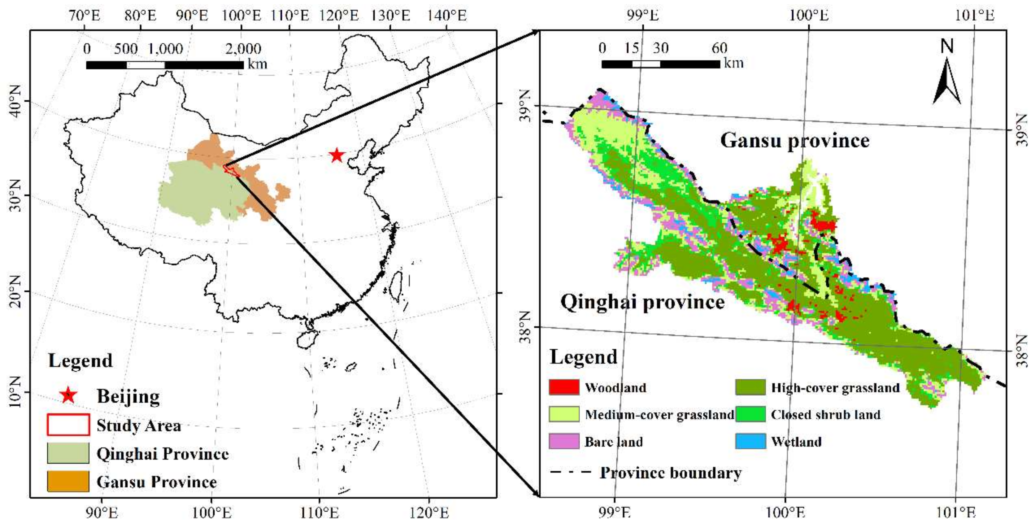
Our study site was located in the upper reaches of the Heihe River Basin. The Heihe River is the second largest inland river in China, originating in the Qilian Mountains and flowing into the Inner Mongolia Plateau. The upper reaches of the Heihe River Basin span between 37.7° N–39.1° N and 98.6° E–101.2° E. Total area is nearly 1 × 10⁶ ha, with 20% located in Gansu Province, and 80% distributed in Qinghai Province (Figure 1). 98.53% of the study area belongs to unpopulated zone. Elevation in the area ranges from 1991 to 4741 m. The region has a typical continental monsoon climate with an annual average temperature of 2.3 °C and an annual average precipitation of 536 mm [35]. Affected by climate, topography and vegetation, the landscape exhibits vertical zones, with mountain deserts and grasslands below 2600 m, conifer/broadleaf mixed forest between 2600–2800 m, Qinghai spruce (Picea crassifolia Kom) forest and alpine shrub land between 3500–4500 m, and alpine desert and glacier above 4500 m [36]. Soil types also display a vertical distribution, with mountain grey calcic soil at 1900–2300 m, chestnut soil at 2300–2600 m, grey cinnamon and chestnut soil at 2600–3200 m, gray brown and mountain black earth soil at 3200–3600 m, alpine shrub meadow soil and alpine shrub grassland soil at 3600–4000 m, and cold desert soil at >4000 m [37].
2.2. Acquisition of Land Cover Data
2.2.1. Historical Land Cover Data
We used 16-day 1000 m MODIS NDIV data (Table 1) to classify land cover types of the study area. First, we transformed the geographic coordinate system to the Universal Transverse Mercator (UTM) projection. While water vapor, bi-directional reflection, aerosol and other factors may affect the accuracy of NDVI data, resulting in difficulties with trend analyses and information extraction [38]. Thus, NDVI data are typically processed to improve classification accuracy. The HANTS smoothing process has the following advantages when dealing with NDVI data: it resolves unequal intervals of time series data, simplifies and compresses time series data, and it detects and replaces invalid data in the time series. In short, the HANTS smoothing process can reconstruct high-quality NDVI timing data [39]. Then we used this method to handle with the obtained MOD13A2 data.
Classification processes include two phases. The first phase involves choosing the classification method. Gu et al. [40] proposed a detailed and effective method to classify land cover types in the Heihe River Basin by analyzing 16-day 1000 m MODIS NDIV data. Thus, we used this classification method to classify land cover types. The second phase involves determination of land cover types. Land cover types in the study area were classified into 6 categories: woodland, closed shrub land, high-cover grassland (cover > 50%), medium-cover grassland (cover between 20% and 50%), wetland and bare land (cover < 20%).
2.2.2. Future Land Cover Data
We used the IDRISI 17.2 software to forecast land cover map for 2029 based on the following 6 steps: (1) Preparation of suitability maps. The Multi-Criteria Evaluation (MCE) module was used to produce suitability maps (Appendix A) by combing driving factors based on certain weights (Appendix B). Besides, the woodland and wetland were constrained to convert to other land cover types based on the goals of local ecological protection and restoration programs. (2) Acquisition of the transition probability matrix through the Markov module in IDRISI 17.2 by inputting land cover maps for 2001 and 2008. (3) Construction of a CA filter. A 5 × 5 contiguity filter was chosen as the neighborhood definition [41]. (4) Simulation of land cover map for 2015. With the suitability maps and transition probability matrix entered into the CA-Markov model, and with the land cover map for 2008 set as the initial year, we simulated the land cover map for 2015 by iterating the module 7 times. (5) Accuracy test. We entered both the simulated and the actual land cover map for 2015 into the VALIDAT module to test the reliability of the CA-Markov model (If the Kappa index > 0.80, it denotes that the CA-Markov model passed the accuracy test) [42]. (6) Prediction of land cover map for 2029. By setting the land cover map for 2015 as the initial year, the land cover map for 2029 was obtained by iterating the CA-Markov model 14 times.
2.3. Estimation of the Total ESV
The benefit transfer method was used to estimate the total ESV; the pre-assigned equivalents were based on Xie et al. [32], who refined the classification of ecosystem services and proposed a set of equivalents applicable to China. The ecosystem was subdivided into 14 sub-types on the basis of the former 6 primary types [43], improving classification of ecosystem services from 9 to 11. The study area is mostly covered by vegetation, and such land cover has 11 types of ecosystem services as proposed by Xie et al. [32]. Moreover, Xie et al. [32] proposed a method for correcting equivalents, which reduced subjectivity of the equivalents derived from expert experience. These corrected equivalents are more suitable for our study area. Data required for correcting equivalents are listed in Table 1.
2.3.1. The Economic Value of One Equivalent
The economic value of one equivalent refers to the net profit from farmland food production per ha per year [32]. Based on the Zhangye Statistical yearbook for 2001–2015, corn, wheat, and potatoes were main crops in the study area. Furthermore, Costanza et al. [31] proposed that there were differences in the levels of economic development among different regions, and the levels of inhabitant understanding of ecosystem services were different. Therefore, the capacity and willingness to pay for ecosystem services should be included in the calculation process. Then, the economic value of one equivalent was calculated by using the following formulas [31,32,47,48]:
where E is the economic value of one equivalent; Pi is the percentage of planting area of crop i; Qi is the net profit for crop i; R is the index of capacity to pay; Y is the index of willingness to pay; GDPm is the real GDP per capita of the study area; GDPn is the real GDP per capita of China; e is the natural logarithm; t is the socioeconomic development index; and En is the Engel coefficient.
2.3.2. Calculation of ESV per ha
We calculated the unit values based on the following formulas, which were proposed by Xie et al. [32].
where Uki is the unit value of ecosystem service i of land cover k; E is the economic value of one equivalent; Dki is the equivalent per ha of ecosystem service i of land cover k [32]; Fki is the functional adjustment index for equivalent of ecosystem service i of land cover k; Ck, Wk, and Mk refer to the average NDVI of growing season, the annual average precipitation, and annual average amount of soil retention of land cover k in the study area, respectively; , , and
represent the corresponding average values in China. Specifically, (1) includes the ecosystem services of food production, raw material, atmosphere regulation, climate regulation, waste treatment, nutrient cycling, biodiversity protection and recreation & culture; (2) includes the ecosystem services of water supply and water regulation; and (3) includes the ecosystem service of soil retention.
2.3.3. Calculation of Total ESV
2.4. Elasticity in ESV in Response to Land Cover Change
Elasticity is a measure of change in economic variables as a function of another variable. In this study, we aimed to assess the responses of ESV to land cover change. Thus, the elasticity indicator was used to measure the percent change in ESV due to percent change in land cover [29].
where EEL is the elasticity of ESV in relation to land cover change; ESVstart and ESVend are the ESVs at the start and the end of the study period, respectively; LCP is the percent of land cover conversion; ΔLUTi is the converted area of land cover i; and LUTi is the total area of land cover i. If EEL > 1, the change in ESV is elastic to land cover change, otherwise, the changes in ESV are considered inelastic to land cover changes.
2.5. Contribution Rates of Land Cover Types to ESV
The contribution rate (CR) is calculated to measure the dependency of ESV on certain land cover type [49]. The larger the CR, the higher the contribution rate of a land cover to ESV.
where CR is the contribution rate; Uk is the unit values of land cover k, Ak is the area of land cover k; ESV is the total ecosystem service value.
3. Results
3.1. Land Cover Change Analyses
3.1.1. Land Cover Change from 2001 to 2015
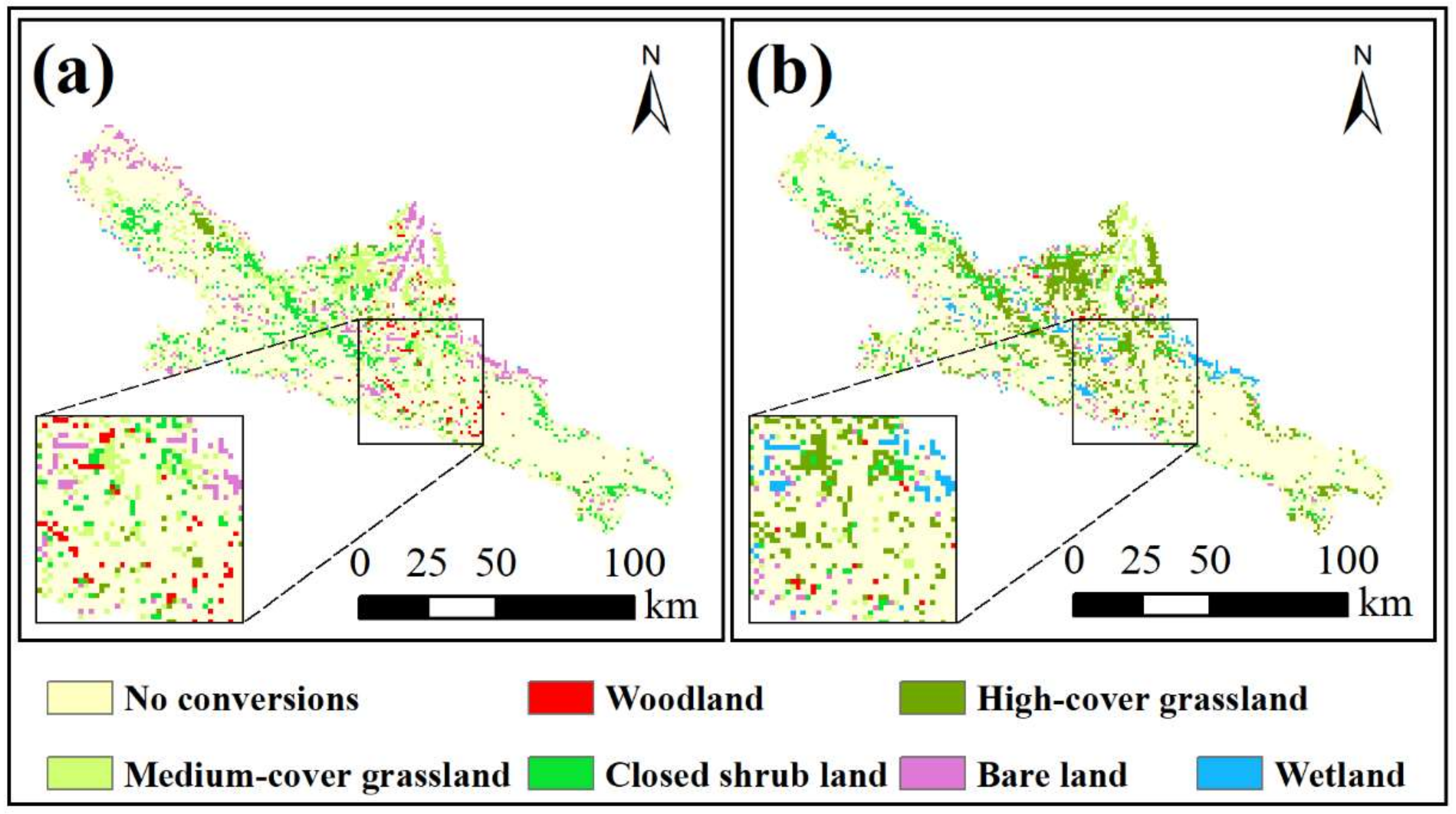
During the period 2001–2015, 25.56% of the total area was converted to other land cover types (Table 2) (Figure 2). The area of high-cover grassland comprised the largest proportion over the period of 2001–2015, at 34.75% in 2001, and at 44.44% in 2015 (Table 3). On the contrary, the area of medium-cover grassland experienced a strongly decreasing trend. Nevertheless, it accounted for the second largest proportion throughout the study period. Next, closed shrub land and bare land exhibited similar quantities. The area of closed shrub land showed a slightly increasing trend over the period of 2001–2008, then decreased rapidly by 18.54% over the second half of the study period. The area of unused land shrank by 24.15% throughout the study period. The least occupied areas were woodland and wetland. The area of woodland experienced a declining trend between 2001 and 2008, but it increased during the subsequent time interval. Wetland expanded substantially from 2001 to 2015 due to the implementation of Wetland Protection Program.
3.1.2. Land Cover Change from 2015 to 2029
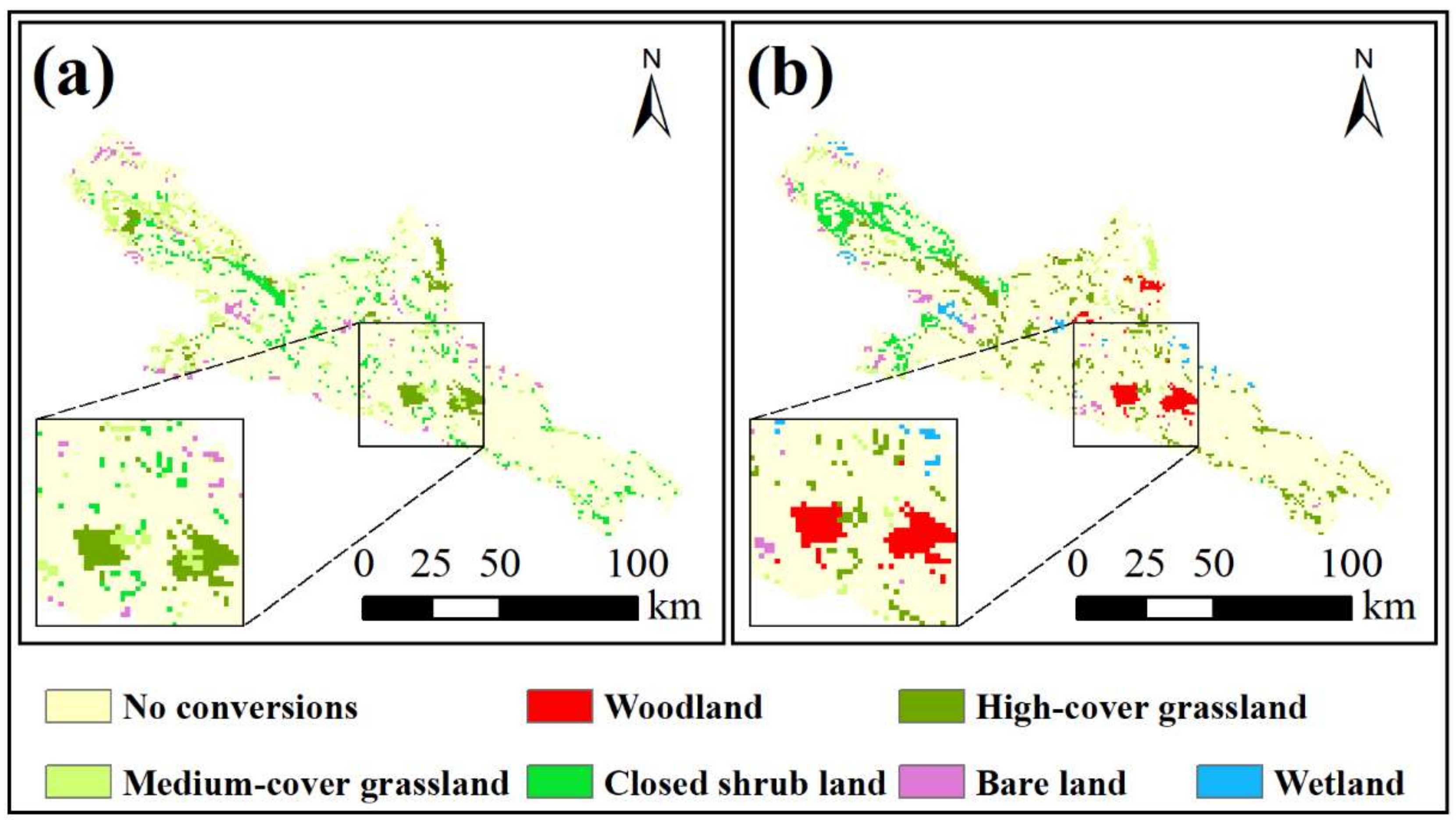
We first tested the simulation accuracy of the CA-Markov model by entering the simulated and actual land cover maps for 2015 into the VALIDAT module in IDRISI 17.2. In addition, the Kappa index was above 0.8000 (0.8370), denoting that the CA-Markov model was highly applicable for simulation of land cover maps in the study area. Thus, we forecasted the land cover map for 2029 with this model. The results showed that if current trends persisted, 16.15% of total area was expected to convert to other land cover types during the period of 2015–2029 (Table 2) (Figure 3). The trend in land cover change of the period of 2015–2029 was highly consistent with the period of 2008–2015: the woodland, high-cover grassland, and wetland were expected to continue expanding in varying degrees, especially in woodland, which was expected to increase by 86.23% (mainly due to conversion from high-cover grassland); the medium-cover grassland, closed shrub land, and bare land were expected to decrease by 16.35%, 8.88% and 4.87%, respectively.
3.2. Changes in ESV from 2001–2029
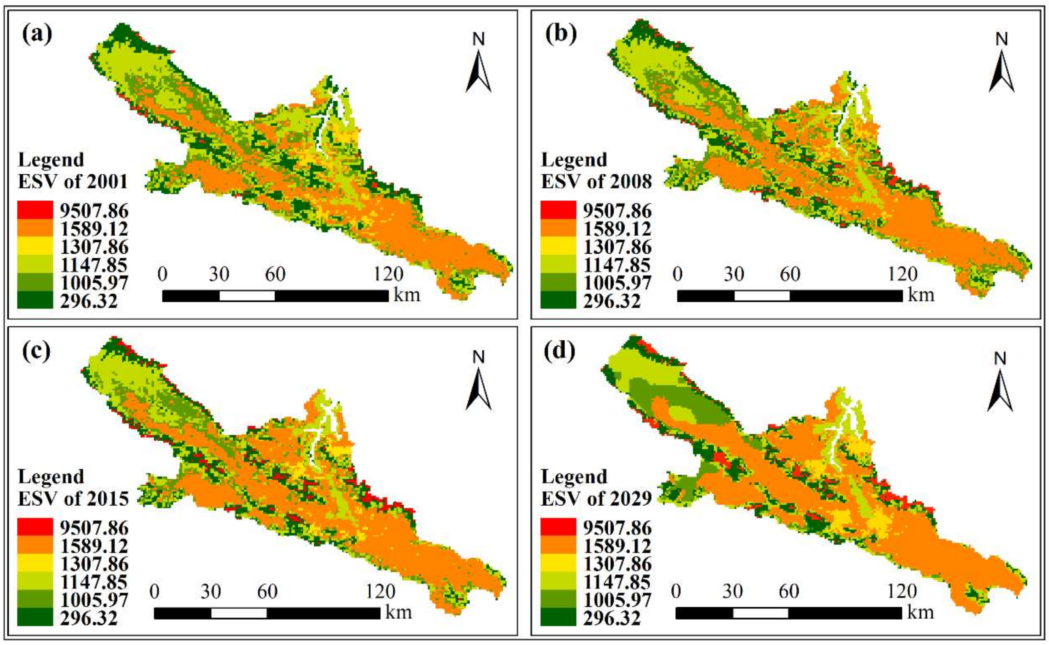
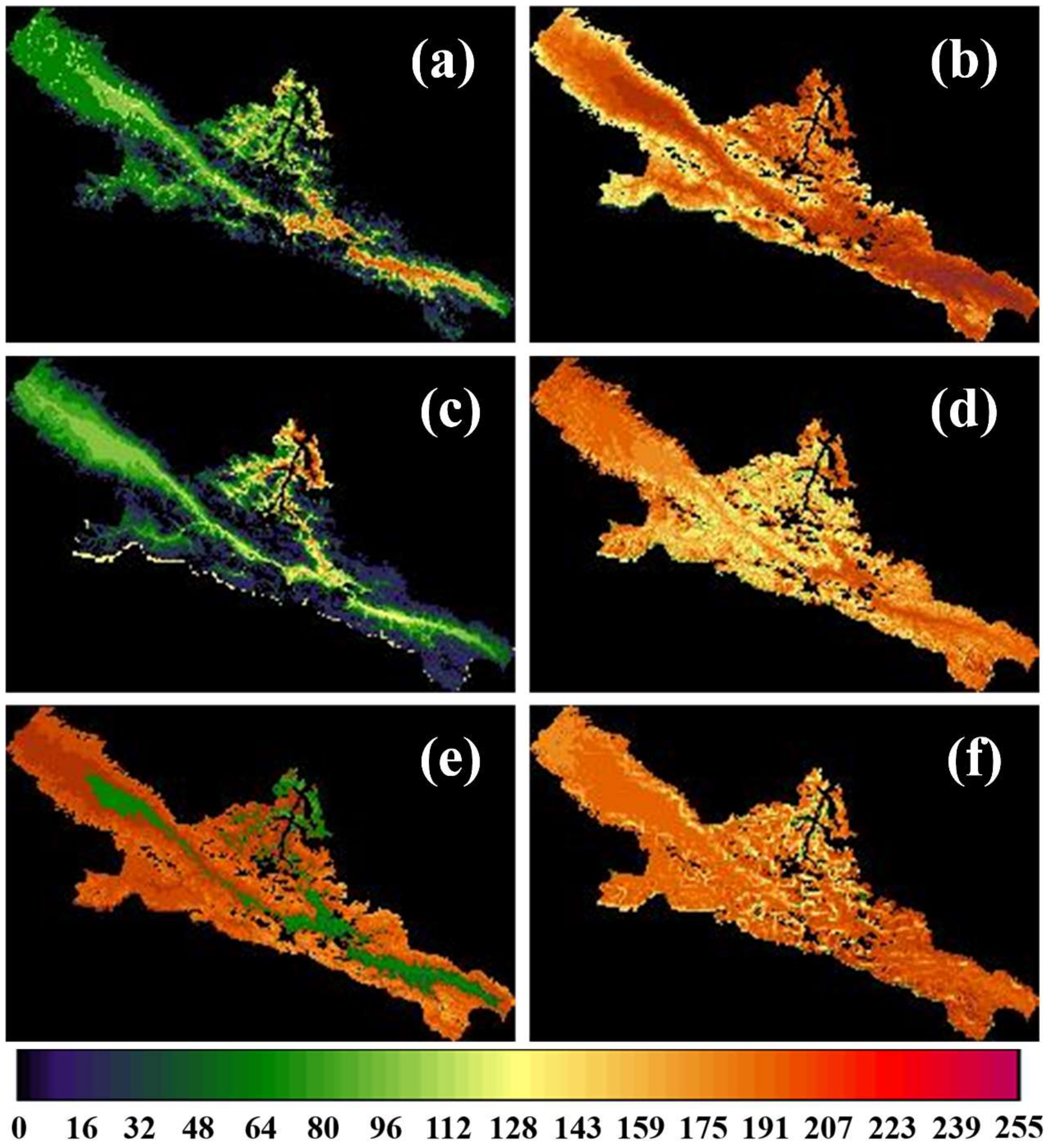
The unit values of each ecosystem service for each land cover type are shown in Table 4. Then the ESVs of 2001, 2008, 2015 and 2029 were calculated, respectively. Our results showed that total ESV of the upper reaches of the Heihe River Basin increased from $1207.33 million (USD) in 2001 to $1,479.48 million (USD) in 2015, and was expected to peak at $1574.53 million (USD) in 2029. The spatial distribution of ESV in the study area showed a trend of high in the southeast and low in the northwest (Figure 4). The ESV of high-cover grassland comprised the largest proportion of the total ESV, and the proportions from 2001 to 2029 had similar quantities (44.56–46.58%) (Figure 5). In addition, the ESV of wetland significantly increased, and its proportions increased from 7.95% in 2001 to 20.79% in 2015, and finally 25.84% in 2029. This was followed by medium-cover grassland, which accounted for more than 14.10% of the total ESV over the study period. Similarly, the proportions of ESV of closed shrub land decreased from 12.60% in 2001 to 7.34% in 2029. Finally, both of the ESVs of bare land and woodland represented less than 5% of total ESV throughout the study period.
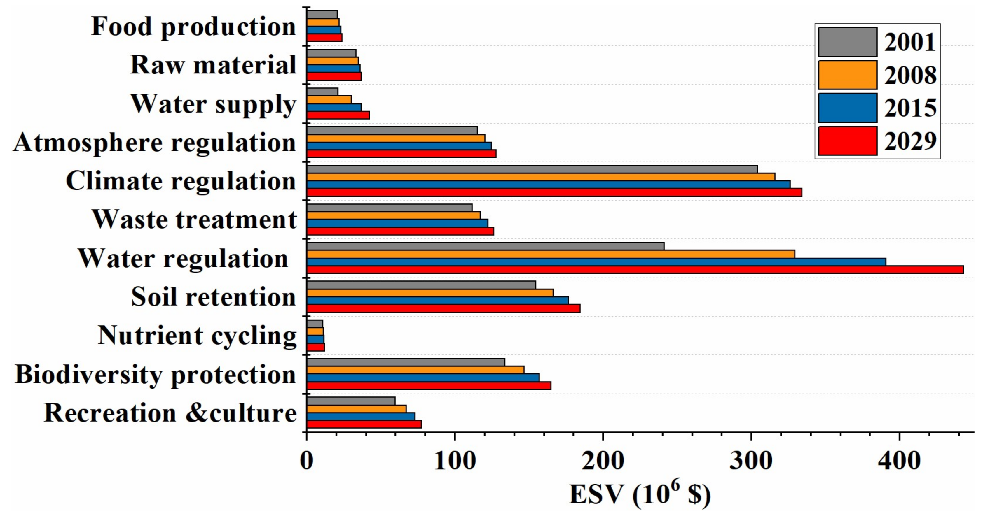
All of the 11 kinds of ESVs increased over the 14 years to varying degrees (Figure 6). The value of water regulation rose dramatically, from 19.98% in 2001 to 26.43% in 2015, and was expected to reach 28.15% in 2029. Additionally, the value of climate regulation experienced a sharp increase, with the figures climbing from $304.20 million (USD) in 2001 to $326.16 million (USD) in 2015, and $334.07 million (USD) in 2029. The values of soil conservation and biodiversity protection represented similar proportions (10–15%). Proportions of the values of gas regulation and waste treatment remained stable (5–10%). The values of the remaining ecosystem services accounted for less than 5% throughout the study period.
3.3. Elasticity of Change in ESV with Respect to Land Cover Chang.
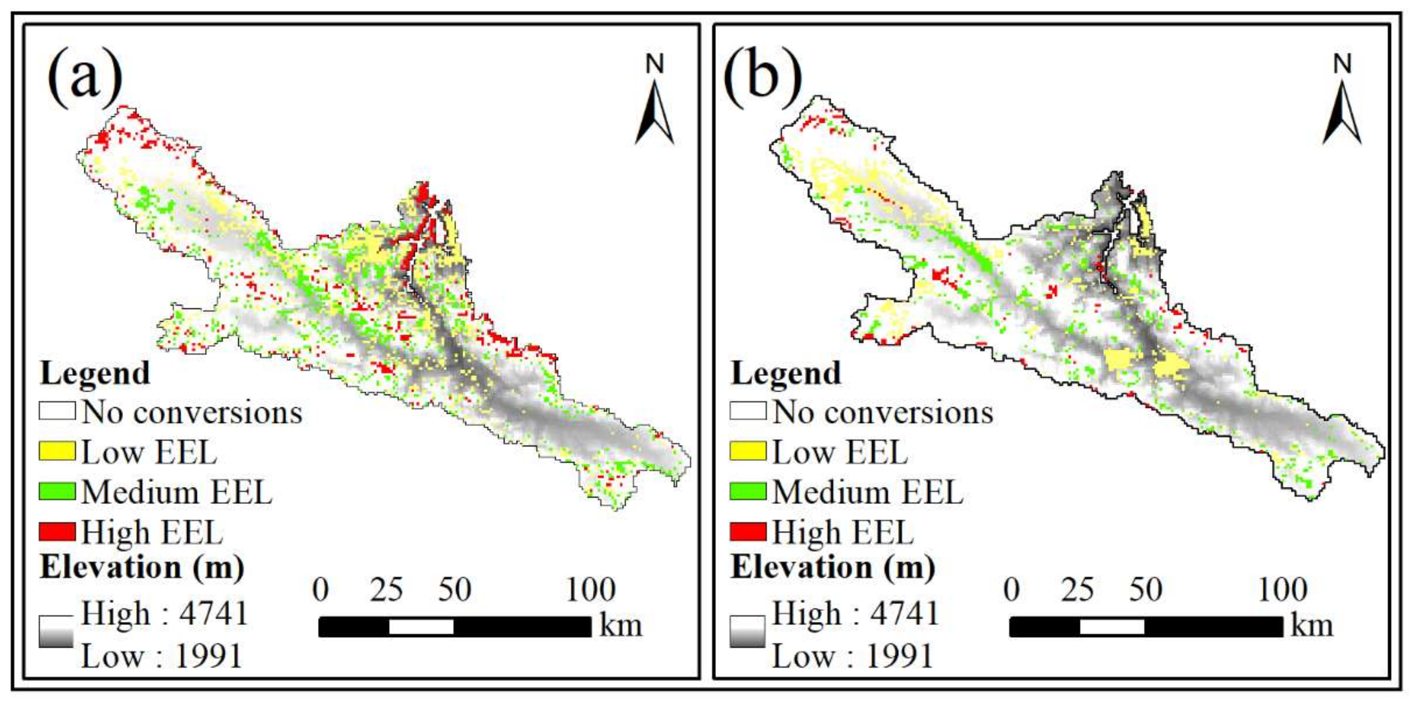
The EELs were categorized into three groups based on their distributions in the study area: EEL ≥ 1 was classified as high, 0.5 < EEL < 1 was classified as medium, 0 < EEL ≤ 0.5 was classified as low. The results showed that the EELs during the periods of 2001–2015 and 2015–2029 were 0.88 and 0.40, respectively (Figure 7), indicating that conversion of 1% of land cover area would result in 0.88% and 0.40% changes in ESV. Responses of ESV to land cover change were not very marked.
Distribution of EELs exhibited noticeable zonality (Figure 8). Namely, the higher the elevation, the higher the EEL. With an increase in elevation in the alpine area, the temperature decreased, while precipitation increased to varying degrees. Consequently, the distribution of EELs was negatively correlated with temperature, and positively with precipitation.
3.4. Analyses of Contribution Rates of Land Cover Types to ESV
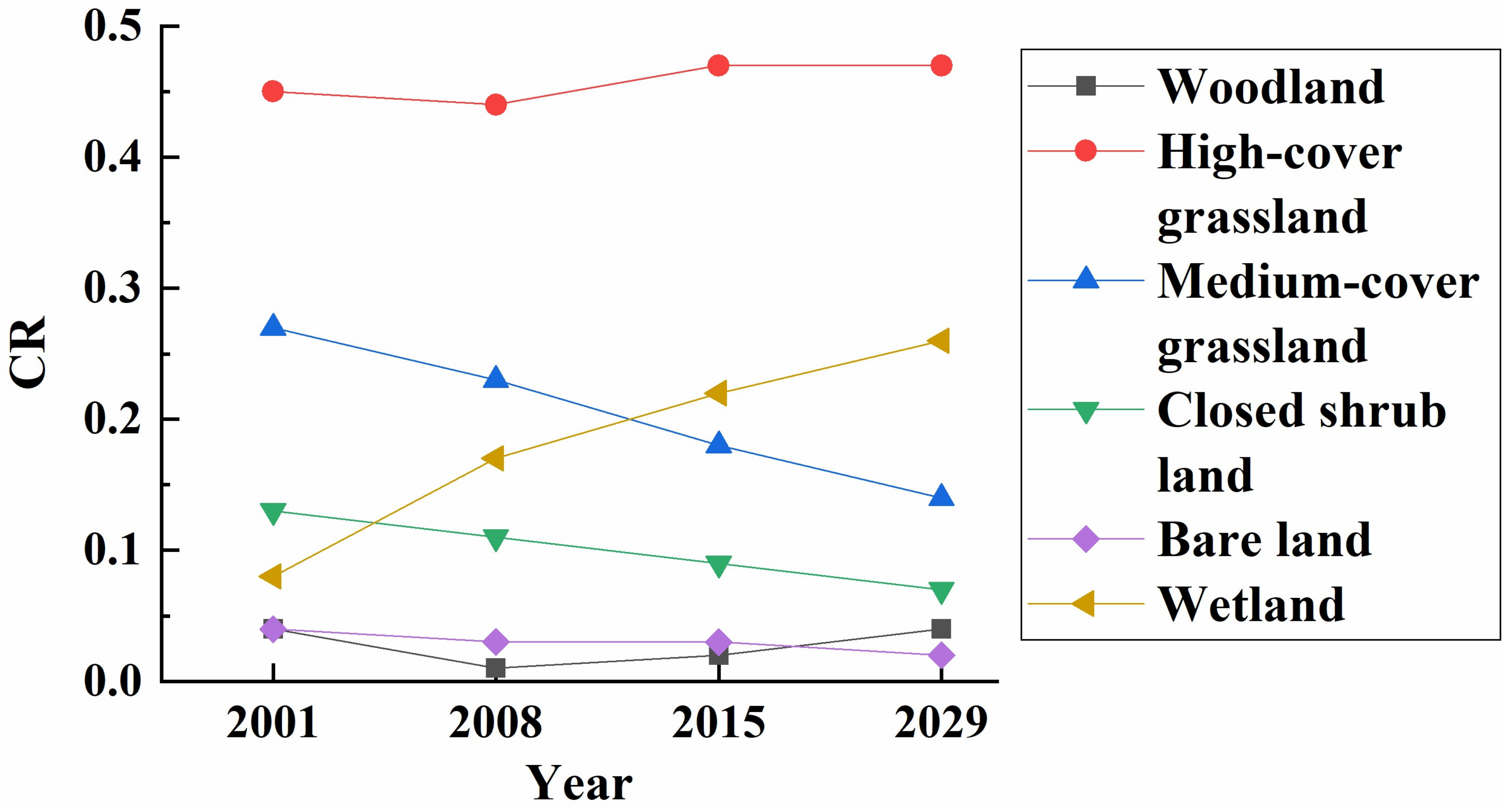
CRs (Figure 9) were calculated to measure the contribution rate of a land cover type to ESV. The results showed that CRs of high-cover grassland and wetland were relatively higher than those of other land cover types, partly because the area of high-cover grassland represented the largest proportion, and partly because its unit values were higher than those of other land cover types. Wetland CRs were expected to increase from 0.08 in 2001 to 0.26 in 2029 along with expansion of its area. Though the CR of medium-cover grassland was 0.27 in 2001, its value was expected to decrease to 0.14 in 2029. The CRs of other land cover types were close to zero. These results demonstrated that an accurate correction of coefficients of high-cover grassland and wetland were critical for the estimation of the total ESV in the upper reaches of the Heihe River Basin.
4. Discussion
4.1. Effects of Land Cover Change on ESV
Presently, ecological protection and restoration is more and more relevant than ever since appeals for sustainable development is increasing. Considerable investments in these programs have changed the landscape pattern. The cumulative land cover changes alter ecosystem structure and function [50]. In our study, area, the land cover pattern from 2001 to 2015 was also optimized due to implantation of ecological protection and restoration programs, and the total ESV increased by $272.15 million (USD). Conversion from bare land to wetland added ESV of $233.97 million (USD). Besides, conversions from closed shrub land and medium-cover grassland to high-cover grassland increased ESV by $53.83 million (USD). Nevertheless, conversions from wetland and medium-cover grassland to bare land still existed, leading to an ESV losses of $31.65 million (USD).
In the near future, the total ESV of the study area was expected to increase by $95.05 million (USD) from 2015 to 2029. Similar to the previous time interval (2001–2015), the increase in ESV was expected to mainly result from wetland expansion. Conversion from bare land to wetland was expected to increase ESV of $82.90 million (USD). In addition, closed shrub land and medium-cover grassland were expected to convert to high-cover grassland, resulting in an ESV increase of $32.09 million (USD). In addition, vegetation degradation was expected to be main cause for loss of ESV. Conversions of high-cover grassland to other vegetation types were expected to account for the largesse loss of ESV, $13.55 million (USD). Degradation of medium-cover grassland to bare land was expected to lead to an ESV loss of $10.39 million (USD).
In all, due to the implementation of ecological protection programs, land cover types with lower unit values (e.g., medium-cover grassland, bare land) were converted to those with higher unit values (e.g., high-cover grassland, wetland). In particular, the conversion of bare land to wetland contributed most to the increase of ESV. While vegetation degradation (e.g., high-cover grassland to medium-cover grassland, medium-cover grassland to bare land) was main cause for loss of ESV. This issue should be taken seriously to prevent further loss of ESV.
4.2. Comparisons with Other Results
Comparison with published results was a feasible way to assess the reasonableness of our approach. It was worth noting that because we calculated the comparable value relative to 2001, we chose the year 2001 as the base year for compared to other studies. Research on the ESV in China reached its peak in 2010 [32]. Presently, most Chinese studies are restricted to certain ecosystem types [51], certain areas [52], or including China as a whole [53]. Though several studies are conducted on the ESV of the Heihe River Basin, their focus is the middle [54], and the lower reaches [55], which have a higher intensity of human activity. Even though there are already a small number of studies on the upper reaches, research has focused on specific ecosystem services, not on total ESV [56]. Therefore, we only compared our results with those of Zhang et al. [57]. The results of Zhang et al. [57] showed that the ESV in the upper reaches of the Heihe River Basin in 2000 was $339.20 million (USD), which was 28.20% of that for our study. The main reasons for the differences were: Zhang et al. [57] calculated ESV based on the unit values of Costanza et al. [31]. However, the unit values in Costanza et al. [31] were not applicable to the study area. The adjusted unit values in our study were higher than those of Costanza et al. [31], partly because we calculated the ESVs of 11 ecosystem services, rather than 9 in Costanza et al. [31], partly because the equivalents from Xie et al. [32] were higher than those from Costanza et al. [31].
Furthermore, we compared our results with Shi et al. [53], who estimated the ESV of China based on the 1999 unit values. Overall, the unit values in our study were similar to those of Shi et al. [53]. Specifically, the unit values of woodland in our study were lower than the value from Shi et al. [53], which was due to forest type in the study area were coniferous forest and closed shrub, with lower unit values than that of broad-leaved forest and coniferous and broad-leaved mixed forest in other regions of China [32]. In contrast, the unit values of high-cover and medium-cover grassland were higher than that of the average level of China. This was principally because the main type of grassland in our study area was meadow, and its unit values were higher than steppe [32]. Finally, the unit values of wetland were significantly higher than those of other studies. This was due to the fact that in recent years scholars had attached importance to ESV of wetland in recent years, resulting in high equivalents of wetland [32,58,59]. Last, the unit values of unused land were higher, mainly because we incorporated low cover meadow into unused land, enhancing the ability of unused land to provide ecosystem services.
Our results can also be verified by comparing them with areas in the world where ecological protection and restoration programs have been implemented. Adusumilli [59] found that the Wetlands Mitigation Program in the United States was very beneficial for improvements in regional ESV. Chazdon’s [60] findings suggested that the woodland can enhance biodiversity conservation and improve ecosystem services. Namely, after implementing ecological protection and restoration programs, ecological land, such as wetland and woodland, usually expanded, and then improved the regional ESV. On the contrary, the ESVs declined in areas where ecological management measures were lacking [58,61,62]. Economic development was always the dominant factor in land use/cover change in those areas [63], and the lack of alternative economic measures has become an important cause of land degradation and ecosystem service reduction. Thus, provisions of effective ecological management, and establishment of a compensation mechanism were considered as essential measures in optimizing land use/cover pattern, and maintaining ecosystem services [64,65].
4.3. Application in Planning for Ecological Management
Assessments of ESV are always applied in spatial planning [66]. The results in this study can be used to support spatial planning and decision-making. Since the study area is belong to the Qilian Mountain Nature Reserve, 98.53% of the total areas are unpopulated. Planning in the study area involves only ecological management. Therefore, the ESV can only be used to adjust the existing ecological management measures and provide suggestions for future ecological management.
First, the ESV can be used as an information source for evaluating impacts of proposed planning decisions [67]. In the Qilian Mountain Nature Reserve, a series of ecological protection and restoration programs are implemented simultaneously, including the Wetland Protection Program, and the Natural Forest Conservation Program. Based on our results, remarkable achievements had been gained of the Wetland Protection Program as the area of wetland increased from 101 ha in 2001 to 340 ha in 2015. In addition, wetland expansion contributed most to the growth of ESV. Obviously, investment in Wetland Protection Program has the highest yield to ESV. In the future, the Wetland Protection Program should still be implemented in accordance with present measures. Contrarily, the Natural Forest Conservation Program was not very effective in protecting forest. The woodland shrunk by 23.77% from 2001 to 2015. Specifically, the area of woodland first decreased (2001–2008) and then increased (2008–2015). Obviously, the measures for woodland protection in 2008–2015 were more effective than the former time interval, which was of reference for the Natural Forest Conservation Program.
Second, the EELs can help identify areas of particular environmental sensitivity, and provide strategies for further ecological management [67]. With increasing elevation, increasing precipitation and decreasing temperature, the EELs increased significantly, indicating that the ESVs of those areas were more sensitive to land cover change resulting from these programs. As a result of the Wetland Protection Program, wetland expansion mainly contributed to high EELs. Though current ecological protection and restoration programs had achieved success in the region, further attention should be given to those areas because of the responses they have shown [29]. While the medium EEL was mainly caused by vegetation degradation (medium-grassland converting to bare land), the focus of ecological management in these regions should be to prevent further deterioration of medium-cover grassland. In summary, the focus of ecological management in the study area is to support the current protection measures, and prevent vegetation degeneration in ecologically fragile areas.
4.4. Limitations of ESV Evaluation
In this study, we applied the benefit transfer method to assess the effects of land cover change on ESV, which is popular with decision makers in virtue of fast evaluation and low demand for data when assessing ESV at broad geographical scales [29]. Nevertheless, limitations of the benefit transfer method still exist. First, we applied pre-assigned parameters that were previously reported for assessing ESV. Although we adjusted them in the application process, the results were still an estimation and simulation of the real situations. Additionally, terrestrial ecosystem supplies not only positive services, but also negative ones [53]. Taking artificial ecosystems as an example, construction land supplies the ecosystem services of recreation & culture and waste treatment, meanwhile, it changes the original natural landscape, and obstructs the original ecological process [68]. Therefore, neglecting negative ecosystem services may cause deviations in the evaluation of ESV [69]. Regarding further research on ESV, the empirical parameters should be determined more accurately based on local conditions. In addition, a greater effort should be made to incorporate the positive and negative ecosystem services into the accounting method of ESV to measure ESV accurately and comprehensively.
5. Conclusions
The effects of land cover change on ESV in the upper reaches of the Heihe River Basin were assessed in northwestern China. The results showed that from 2001 to 2015, the land cover types with lower unit values (e.g., medium-cover grassland, bare land) were converted to those with higher unit values (e.g., high-cover grassland, wetland). In addition, the trend of land cover change from 2015 to 2029 is expected to be similar to that of 2001–2015.
Due to land cover change, the total ESV of the study area increased from $1207.33 million (USD) in 2001 to $1479.48 million (USD) in 2015, and the value was expected to reach $1574.53 million (USD) in 2029. Along with those, the ESVs of 11 types of ecosystem services showed increasing trends to varying degrees, especially those of water and climate regulation due to expansions of wetland and high-cover grassland.
The EEL was also adopted to assess the response of ESV to land cover change, and the results showed that the values were 0.88% and 0.40% during 2001–2015 and 2015–2029, respectively. Moreover, high EELs were distributed in regions with higher elevation, more precipitation and lower temperature.
In this study, areas sensitive to ecological protection and restoration are identified. This will aid in selecting representative sites from the alpine zones for further ecological management. Furthermore, the results of changes in ESV will support decision-making in trade-offs involved in environmental management. However, only the positive ecosystem service values were evaluated. In the future, efforts should be paid to incorporate the negative and positive ecosystem services into the accounting method for ESVs.
Author Contributions
Conceptualization, M.Z. and Z.H.; methodology, M.Z.; software, M.Z.; validation, Z.H.; formal analysis, M.Z.; investigation, M.Z.; resources, Z.H.; data curation, Z.H.; writing—original draft preparation, M.Z.; writing—review and editing, Z.H.; visualization, Z.H.; supervision, Z.H.; project administration, Z.H.; funding acquisition, Z.H.
Funding
This research was funded by the National Natural Science Foundation of China (No. 41621001, 41522102, 41701296 and 41601051).
Acknowledgments
We are grateful to Kathryn Piatek for help with revisions.
Conflicts of Interest
The authors declare no conflict of interest.
Appendix A

Table A1.
Parameters and weights used in simulations of suitability maps.
| Land Cover Types | Consistency Ratio | Variables | Description | Factor Weight | Function Type b |
|---|---|---|---|---|---|
| Woodland | 0.0139 | Temperature | 8.0–14.0 °C, 11 °C a | 0.4175 | SS |
| Precipitation | 320–600 mm, 460 mm a | 0.2241 | SS | ||
| Elevation | 2200–3800 m, 3000 m a | 0.1132 | SS | ||
| Slope | 0°–37° | 0.0575 | DS | ||
| Aspect | 0°–180°; 180°–360° | 0.1876 | DJ;IJ | ||
| High-cover grassland | 0.0116 | Temperature | −5–16 °C | 0.4849 | IS |
| Precipitation | 240–960 mm | 0.2800 | IS | ||
| Elevation | 2000–4800 m, 3500 m a | 0.1669 | SS | ||
| Slope | 0°–37° | 0.0681 | DS | ||
| Medium-cover grassland | 0.0152 | Temperature | −5–16 °C | 0.1605 | IS |
| Precipitation | Less than 600 mm | 0.4881 | DS | ||
| Elevation | Less than 3500 m | 0.2515 | DS | ||
| Slope | 0°–37° | 0.0999 | IS | ||
| Closed shrub land | 0.0250 | Temperature | −5–16 °C | 0.4750 | IS |
| Precipitation | 240–960 mm | 0.1654 | IS | ||
| Elevation | More than 3300 m | 0.3113 | IS | ||
| Slope | 0°–37° | 0.0483 | DS | ||
| Wetland | 0.0000 | Precipitation | 240–960 mm | 0.2857 | IS |
| Elevation | 2000–4800m | 0.1429 | DS | ||
| Slope | 0°–37° | 0.5714 | DS | ||
| Bare land | 0.0000 | Temperature | −5–16 °C | 0.6000 | DS |
| Precipitation | 240–960 mm | 0.3000 | DS | ||
| Slope | 0°–37° | 0.1000 | IS |
Note: a—The value at the symmetry point. b SS—Symmetric sigmoidal function, DS—Decreasing sigmoidal function, IS—Increasing sigmoidal function, IJ—Increasing J—shaped function, DJ—Decreasing J-shaped function.
Appendix B
Figure A1.
Suitability maps of each land cover type: (a)—Woodland, (b)—High-cover grassland, (c)—Medium-cover grassland, (d)—Closed shrub land, (e)—Bare land, (f)—Wetland.
Figure A1.
Suitability maps of each land cover type: (a)—Woodland, (b)—High-cover grassland, (c)—Medium-cover grassland, (d)—Closed shrub land, (e)—Bare land, (f)—Wetland.

References
- Sarukhan, J.; Whyte, A.; Hassan, R.; Scholes, R.; Ash, N.; Carpenter, S.T.; Pingali, P.L.; Bennett, E.M.; Zurek, M.B.; Chopra, K. Millenium Ecosystem Assessment: Ecosystems and Human Well-being; World Resources Inst.: Washington, DC, USA, 2005. [Google Scholar]
- Costanza, R.; Groot, R.D.; Sutton, P.; Ploeg, S.V.D.; Anderson, S.J.; Kubiszewski, I.; Farber, S.; Turner, R.K. Changes in the global value of ecosystem services. Glob. Environ. Chang. 2014, 26, 152–158. [Google Scholar] [CrossRef]
- Farley, J.; Costanza, R.; Farley, J.; Costanza, R. Special Section: Payments for ecosystem services: From local to global. Ecol. Econ. 2010, 69, 2060–2068. [Google Scholar] [CrossRef]
- Braat, L.C.; Groot, R.D. The ecosystem services agenda:bridging the worlds of natural science and economics, conservation and development, and public and private policy. Ecosyst. Serv. 2012, 1, 4–15. [Google Scholar] [CrossRef]
- Finlayson, C.M.; Horwitz, P. Human Health and the Wise Use of Wetlands—Guidance in an International Policy Setting. Wetlands and Human Health; Springer: Dordrecht, The Netherlands, 2016. [Google Scholar]
- Turner, K.G.; Anderson, S.; Gonzales-Chang, M.; Costanza, R.; Courville, S.; Dalgaard, T.; Dominati, E.; Kubiszewski, I.; Ogilvy, S.; Porfirio, L. A review of methods, data, and models to assess changes in the value of ecosystem services from land degradation and restoration. Ecol. Model. 2016, 319, 190–207. [Google Scholar] [CrossRef]
- Lin, X.; Xu, M.; Cao, C.; Singh, R.; Chen, W.; Ju, H. Land-Use/Land-Cover Changes and Their Influence on the Ecosystem in Chengdu City, China during the Period of 1992–2018. Sustainability 2018, 10, 3580. [Google Scholar] [CrossRef]
- Frélichová, J.; Fanta, J. Ecosystem service availability in view of long-term land-use changes: A regional case study in the Czech Republic. Ecosyst. Health Sustain. 2016, 1, 1–15. [Google Scholar] [CrossRef]
- Cegielska, K.; Noszczyk, T.; Kukulska, A.; Szylar, M.; Hernik, J.; Dixongough, R.; Jombach, S.; Valanszki, I.; Kovacs, K.F. Land use and land cover changes in post-socialist countries: Some observations from Hungary and Poland. Land Use Policy 2018, 78, 1–18. [Google Scholar] [CrossRef]
- Mitsch, W.J. What is ecological engineering? Ecol. Eng. 2012, 45, 5–12. [Google Scholar] [CrossRef]
- Liu, J.; Li, S.; Ouyang, Z.; Tam, C.; Chen, X. Ecological and socioeconomic effects of China’s policies for ecosystem services. Proc. Natl. Acad. Sci. United States Am. 2008, 105, 9477. [Google Scholar] [CrossRef]
- Lawler, J.J.; Lewis, D.J.; Nelson, E.; Plantinga, A.J.; Polasky, S.; Withey, J.C.; Helmers, D.P.; Martinuzzi, S.; Pennington, D.; Radeloff, V.C. Projected land-use change impacts on ecosystem services in the United States. Proc. Natl. Acad. Sci. United States Am. 2014, 111, 7492–7497. [Google Scholar] [CrossRef] [PubMed] [Green Version]
- Zhang, S.; Fan, W.; Li, Y.; Yi, Y. The influence of changes in land use and landscape patterns on soil erosion in a watershed. Sci. Total. Environ. 2017, 574, 34–45. [Google Scholar] [CrossRef] [PubMed]
- Benini, L.; Bandini, V.; Marazza, D.; Contin, A. Assessment of land use changes through an indicator-based approach: A case study from the Lamone river basin in Northern Italy. Ecol. Indic. 2010, 10, 4–14. [Google Scholar] [CrossRef]
- Geneletti, D. Assessing the impact of alternative land-use zoning policies on future ecosystem services. Environ. Impact Assess. Rev. 2013, 40, 25–35. [Google Scholar] [CrossRef]
- Ouyang, Z.; Zheng, H.; Xiao, Y.; Polasky, S.; Liu, J.; Xu, W.; Wang, Q.; Zhang, L.; Xiao, Y.; Rao, E. Improvements in ecosystem services from investments in natural capital. Science 2016, 352, 1455–1459. [Google Scholar] [CrossRef] [PubMed]
- Zhao, C.; Nan, Z.; Cheng, G. Methods for modelling of temporal and spatial distribution of air temperature at landscape scale in the southern Qilian mountains, China. Ecol. Model. 2005, 189, 209–220. [Google Scholar]
- Tallis, H.; Polasky, S. Mapping and valuing ecosystem services as an approach for conservation and natural-resource management. Ann. N. Y. Acad. Sci. 2009, 1162, 265–283. [Google Scholar] [CrossRef]
- Brown, D.G.; Verburg, P.H.; Pontius, R.G.; Lange, M.D. Opportunities to improve impact, integration, and evaluation of land change models. Curr. Opin. Environ. Sustain. 2013, 5, 452–457. [Google Scholar] [CrossRef]
- Salata, S. Land use change analysis in the urban region of Milan. Manag. Environ. Qual. Int. J. 2017, 28, 879–900. [Google Scholar] [CrossRef]
- Ronchi, S.; Salata, S.; Arcidiacono, A. An indicator of urban morphology for landscape planning in Lombardy (Italy). Manag. Environ. Qual. Int. J. 2018, 29, 623–642. [Google Scholar] [CrossRef]
- Salata, S. Land take in the Italian Alps: Assessment and proposals for further development. Manag. Environ. Qual. Int. J. 2014, 25, 407–420. [Google Scholar] [CrossRef]
- Noszczyk, T. A review of approaches to land use changes modeling. Hum. Ecol. Risk Assess. 2018. [CrossRef]
- Dang, A.N.; Kawasaki, A. A Review of Methodological Integration in Land-Use Change Models. Int. J. Agric. Environ. Inf. Syst. 2017, 7. [Google Scholar] [CrossRef]
- He, C.; Zhang, D.; Huang, Q.; Zhao, Y. Assessing the potential impacts of urban expansion on regional carbon storage by linking the LUSD-urban and InVEST models. Environ. Model. Softw. 2016, 75, 44–58. [Google Scholar] [CrossRef]
- Anputhas, M.; Janmaat, J.; Nichol, C.F.; Wei, X.A. Modelling spatial association in pattern based land use simulation models. J. Environ. Manag. 2016, 181, 465–476. [Google Scholar] [CrossRef] [PubMed]
- Basse, R.M.; Omrani, H.; Charif, O.; Gerber, P.; Bódis, K. Land use changes modelling using advanced methods: Cellular automata and artificial neural networks. The spatial and explicit representation of land cover dynamics at the cross-border region scale. Appl. Geogr. 2014, 53, 160–171. [Google Scholar] [CrossRef]
- Nor, A.N.M.; Corstanje, R.; Harris, J.A.; Brewer, T. Impact of rapid urban expansion on green space structure. Ecol. Indic. 2017, 81, 274–284. [Google Scholar] [CrossRef]
- Song, W.; Deng, X. Land-use/land-cover change and ecosystem service provision in China. Sci. Total. Environ. 2017, 576, 705–719. [Google Scholar] [CrossRef]
- Crossman, N.D.; Burkhard, B.; Nedkov, S.; Willemen, L.; Petz, K.; Palomo, I.; Drakou, E.G.; Martín-Lopez, B.; Mcphearson, T.; Boyanova, K. A blueprint for mapping and modelling ecosystem services. Ecosyst. Serv. 2013, 4, 4–14. [Google Scholar] [CrossRef]
- Costanza, R.; D’Arge, R.; Groot, R.D.; Farber, S.; Grasso, M.; Hannon, B.; Limburg, K.; Naeem, S.; O’Neill, R.V.; Paruelo, J. The value of the world’s ecosystem services and natural capital 1. Nature 1997, 387, 3–15. [Google Scholar] [CrossRef]
- Xie, G.D.; Zhang, C.X.; Zhang, L.M.; Chen, W.H.; Shi-Mei, L.I. Improvement of the evaluation method for ecosystem service value based on per unit area. J. Nat. Resour. 2015, 30, 1243–1254. [Google Scholar]
- Benayas, J.M.R.; Bullock, J.M. Enhancement of biodiversity and ecosystem services by ecological restoration: A meta-analysis. Science 2009, 325, 1121–1124. [Google Scholar] [CrossRef] [PubMed]
- Li, F.; Zhang, S.; Yang, J.; Chang, L.; Yang, H.; Bu, K. Effects of land use change on ecosystem services value in West Jilin since the reform and opening of China. Ecosyst. Serv. 2018, 31, 12–20. [Google Scholar]
- Yang, D.; Gao, B.; Jiao, Y.; Lei, H.; Zhang, Y.; Yang, H.; Cong, Z. A distributed scheme developed for eco-hydrological modeling in the upper Heihe River. Sci. China Earth Sci. 2015, 58, 36–45. [Google Scholar] [CrossRef]
- Ding, S.; Su, P. Altitudinal variation characteristics of the plant community on the upper reaches of Heihe River in the Qilian Mountains. J. Glaciol. Geocryol. 2010, 32, 829–836. [Google Scholar]
- Wang, C. The Impact of Vegetation Change on Rainfall-runoff Process in Tianlaochi Catchment in Heihe River Basin. Ph.D. Theisi, Lanzhou University, Lanzhou, China, 2013. [Google Scholar]
- Sellers, P.; Tucker, C.; Collatz, G.; Los, S.; Justice, C.; Dazlich, D.; Randall, D. A global 1 by 1 NDVI data set for climate studies. Part 2: The generation of global fields of terrestrial biophysical parameters from the NDVI. Int. J. Remote Sens. 1994, 15, 3519–3545. [Google Scholar] [CrossRef]
- Na, X.; Zhang, S.; Li, X.; Qin, X. Application of MODIS NDVI time series to extracting wetland vegetation information in the Sanjiang Plain. Wetl. Sci. 2007, 5, 227–236. [Google Scholar]
- Gu, J.; Li, X.; Huang, C. Land cover classification based on time-series MODIS NDVI data in Heihe River Basin. Adv. Earth Sci. 2010, 25, 317–326. [Google Scholar]
- Gong, W.; Yuan, L.; Fan, W.; Stott, P. Analysis and simulation of land use spatial pattern in Harbin prefecture based on trajectories and cellular automata—Markov modelling. Int. J. Appl. Earth Obs. Geoinf. 2015, 34, 207–216. [Google Scholar] [CrossRef]
- Zhang, R.; Tang, C.; Ma, S.; Yuan, H.; Gao, L.; Fan, W. Using Markov chains to analyze changes in wetland trends in arid Yinchuan Plain, China. Math. Comput. Model. 2011, 54, 924–930. [Google Scholar] [CrossRef]
- Xie, G.D.; Lin, Z.; Chun-Xia, L.U.; Yu, X.; Cao, C. Expert knowledge based valuation method of ecosystem services in China. J. Nat. Resour. 2008, 23, 911–919. [Google Scholar]
- National Aeronautics and Space Administration (NASA). The Atmosphere Archive and Distribution System (LAADS). Available online: http://ladsweb.nascom.nasa.gov (accessed on 12 February 2016).
- Data Center for Resources and Environmental Sciences, Chinese Academy of Sciences (RESDC). Spatial interpolation data set of annual precipitation in China since 1980. Available online: http://www.resdc.cn (accessed on 5 June 2016).
- Data Center for Resources and Environmental Sciences, Chinese Academy of Sciences (RESDC). Spatial Distribution Data Set of Terrestrial Ecosystem Service Value in China. Available online: http://www.resdc.cn (accessed on 21 July 2016).
- Fu, B.; Li, Y.; Wang, Y.; Zhang, B.; Yin, S.; Zhu, H.; Xing, Z. Evaluation of ecosystem service value of riparian zone using land use data from 1986 to 2012. Ecol. Indic. 2016, 69, 873–881. [Google Scholar] [CrossRef]
- Kwasnicki, W. Logistic growth of the global economy and competitiveness of nations. Technol. Forecast. Soc. Chang. 2013, 80, 50–76. [Google Scholar] [CrossRef]
- Aschonitis, V.G.; Gaglio, M.; Castaldelli, G.; Fano, E.A. Criticism on elasticity-sensitivity coefficient for assessing the robustness and sensitivity of ecosystem services values. Ecosyst. Serv. 2016, 20, 66–68. [Google Scholar] [CrossRef] [Green Version]
- Xiong, X.; Grunwald, S.; Myers, D.B.; Ross, C.W.; Harris, W.G.; Comerford, N.B. Interaction effects of climate and land use/land cover change on soil organic carbon sequestration. Sci. Total Environ. 2014, 493, 974–982. [Google Scholar] [CrossRef] [PubMed]
- Zhang, B.; Shi, Y.T.; Liu, J.H.; Xu, J.; Xie, G.D. Economic values and dominant providers of key ecosystem services of wetlands in Beijing, China. Ecol. Indic. 2017, 77, 48–58. [Google Scholar] [CrossRef]
- Liu, Y.; Li, J.; Zhang, H. An ecosystem service valuation of land use change in Taiyuan City, China. Ecol. Model. 2012, 225, 127–132. [Google Scholar] [CrossRef]
- Shi, Y.; Wang, R.S.; Huang, J.L.; Yang, W.R. An analysis of the spatial and temporal changes in Chinese terrestrial ecosystem service functions. Chin. Sci. Bull. 2012, 57, 2120–2131. [Google Scholar] [CrossRef] [Green Version]
- Liang, Y. Economic valuation of ecosystem service in the middle basin of Heihe River, northwest China. Int. J. Environ. Eng. Nat. Resour. 2014, 1, 164–170. [Google Scholar]
- Han, Y.W.; Xue-Sen, T.; Gao, J.X.; Liu, C.C.; Gao, X.T. Assessment on the sand-fixing function and its value of the vegetation in eco-function protection areas of the lower reaches of the Heihe River. J. Nat. Resour. 2011, 26, 58–65. [Google Scholar]
- Geng, X.; Wang, X.; Yan, H.; Zhang, Q.; Jin, G. Land use/land cover change induced impacts on water supply service in the upper reach of Heihe River Basin. Sustainability 2014, 7, 366–383. [Google Scholar] [CrossRef]
- Zhang, Z.Q.; Xu, Z.M.; Wang, J. Value of the ecosystem services in the Heihe River Basin. J. Glaciol. Geocryol. 2001, 23, 360–366. [Google Scholar]
- Bhatta, L.D.; Chaudhary, S.; Pandit, A.; Baral, H.; Das, P.J.; Stork, N.E. Ecosystem Service Changes and Livelihood Impacts in the Maguri-Motapung Wetlands of Assam, India. Land 2016, 5, 15. [Google Scholar] [Green Version]
- Adusumilli, N. Valuation of Ecosystem Services from Wetlands Mitigation in the United States. Land 2015, 4, 182–196. [Google Scholar] [CrossRef] [Green Version]
- Chazdon, R.L. Beyond Deforestation: Restoring Forests and Ecosystem Services on Degraded Lands. Science 2008, 320, 1458–1460. [Google Scholar] [CrossRef] [PubMed]
- Cabral, P.; Feger, C.; Levrel, H.; Chambolle, M.; Basque, D. Assessing the impact of land-cover changes on ecosystem services: A first step toward integrative planning in Bordeaux, France. Ecosyst. Serv. 2016, 22, 318–327. [Google Scholar] [CrossRef]
- Tolessa, T.; Senbeta, F.; Kidane, M. The impact of land use/land cover change on ecosystem services in the central highlands of Ethiopia. Ecosyst. Serv. 2017, 23, 47–54. [Google Scholar] [CrossRef]
- Noszczyk, T.; Rutkowska, A.; Hernik, J. Determining Changes in Land Use Structure in Małopolska Using Statistical Methods. Pol. J. Environ. Stud. 2017, 26, 211–220. [Google Scholar] [CrossRef] [Green Version]
- Hu, H.; Liu, W.; Cao, M. Impact of land use and land cover changes on ecosystem services in Menglun, Xishuangbanna, Southwest China. Environ. Monit. Assess. 2008, 146, 147–156. [Google Scholar] [CrossRef]
- Wang, Z.; Wang, Z.; Zhang, B.; Lu, C.; Ren, C. Impact of land use/land cover changes on ecosystem services in the Nenjiang River Basin, Northeast China. Ecol. Process. 2015, 4, 11. [Google Scholar] [CrossRef]
- Langemeyer, J.; Gómez-Baggethun, E.; Haase, D.; Scheuer, S.; Elmqvist, T. Bridging the gap between ecosystem service assessments and land-use planning through Multi-Criteria Decision Analysis (MCDA). Environ. Sci. Policy 2016, 62, 45–56. [Google Scholar] [CrossRef]
- Albert, C.; Geneletti, D.; Kopperoinen, L. Application of Ecosystem Services in Spatial Planning; Pensoft Publishers: Sofia, Bulgaria, 2017. [Google Scholar]
- Dong, J.; Shu, T.; Xie, H.; Bao, C. Calculative method for ecosystem services values of urban constructive lands and its application. J. Tongji Univ. 2007, 35, 636–640. [Google Scholar]
- Arnold, J.; Kleemann, J.; Furst, C. A Differentiated Spatial Assessment of Urban Ecosystem Services Based on Land Use Data in Halle, Germany. Land 2018, 7, 101. [Google Scholar] [CrossRef]
Figure 1.
Location and land cover pattern of the study area.

Figure 2.
Land cover change from 2001 to 2015: (a) Land cover pattern in 2001, (b) Land cover pattern in 2015.
Figure 2.
Land cover change from 2001 to 2015: (a) Land cover pattern in 2001, (b) Land cover pattern in 2015.

Figure 3.
Land cover change from 2015 to 2029: (a) Land cover pattern in 2015, (b) Land cover pattern in 2029.
Figure 3.
Land cover change from 2015 to 2029: (a) Land cover pattern in 2015, (b) Land cover pattern in 2029.

Figure 4.
Changes in ESV ($) in the upper reaches of the Heihe River Basin from 2001 to 2029: (a) ESV in 2001, (b) ESV in 2015, (c) ESV in 2015, (d) ESV in 2029.
Figure 4.
Changes in ESV ($) in the upper reaches of the Heihe River Basin from 2001 to 2029: (a) ESV in 2001, (b) ESV in 2015, (c) ESV in 2015, (d) ESV in 2029.

Figure 5.
The ESV for each land cover type in the upper reaches of the Heihe River Basin from 2001 to 2029 (106$).
Figure 5.
The ESV for each land cover type in the upper reaches of the Heihe River Basin from 2001 to 2029 (106$).

Figure 6.
The ESV for each ecosystem service type in the upper reaches of the Heihe River Basin from 2001 to 2029 (106$).
Figure 6.
The ESV for each ecosystem service type in the upper reaches of the Heihe River Basin from 2001 to 2029 (106$).

Figure 7.
Changes in EELs in the upper reaches of the Heihe River Basin from 2001 to 2029: (a) EELs of 2001–2015, (b) EELs of 2015–2029.
Figure 7.
Changes in EELs in the upper reaches of the Heihe River Basin from 2001 to 2029: (a) EELs of 2001–2015, (b) EELs of 2015–2029.

Figure 8.
The environmental factors corresponding to EEL categories in the upper reaches of the Heihe River Basin from 2001 to 2029: (a) Average elevations of 2001–2015, (b) Average elevations of 2015–2029, (c) Annual average temperatures of 2001–2015, (d) Annual average temperatures of 2015–2029, (e) Annual average precipitations of 2001–2015, (f) Annual average precipitations of 2015–2029.

Figure 9.
The CRs of different land cover types from 2001 to 2029.

Table 1.
Database used for calculating ESV.
| Variables | Description | Source |
|---|---|---|
| NDVI | Average value for the growing season (from May to October) | Derived from the Atmosphere Archive and Distribution System (LAADS) [44] |
| Precipitation | Annual average precipitation | Derived from Chinese Academy of Sciences Resource and Environment Science Data Center [45] |
| Amount of soil retention | Calculated with the universal soil loss equation | Derived from Chinese Academy of Sciences Resource and Environment Science Data Center [46] |
| Real GDP per capita | Ratio of total GDP to the total population | Zhangye Statistical yearbook for 2001 |
| The Engel coefficient | Proportion of total expenditure for food to the total expenditure for personal consumption | Zhangye Statistical yearbook for 2001 |
| Crop planting area | The planting area of each crop | Zhangye Statistical yearbook for 2001 |
| Net profit of crop | Net profit per ha obtained by planting crop | Compilation of National Agricultural Product Cost and Income Data for 2001 |
Table 2.
The LCPs, changes in ESV and EELs of periods of 2001–2015 and 2015–2029(103 ha).
| Time Interval | LCP (%) | Changes in ESV (106$) | EEL |
|---|---|---|---|
| 2001–2015 | 25.56 | 272.15 | 0.88 |
| 2015–2029 | 16.15 | 95.05 | 0.40 |
Table 3.
Land cover changes between 2001 and 2029 (103 ha).
| Land Cover Types | 2001 | 2008 | 2015 | 2029 | ||||
|---|---|---|---|---|---|---|---|---|
| Area | % | Area | % | Area | % | Area | % | |
| Woodland | 32.40 | 3.30 | 13.50 | 1.38 | 24.70 | 2.52 | 46.00 | 4.69 |
| High-cover grassland | 341.10 | 34.75 | 380.30 | 38.74 | 436.30 | 44.44 | 461.50 | 47.01 |
| Medium-cover grassland | 284.60 | 28.99 | 275.90 | 28.10 | 231.20 | 23.55 | 193.40 | 19.70 |
| Closed shrub land | 151.20 | 15.40 | 154.80 | 15.77 | 126.10 | 12.85 | 114.90 | 11.70 |
| Bare land | 162.30 | 16.53 | 133.10 | 13.56 | 129.40 | 13.18 | 123.10 | 12.54 |
| Wetland | 10.10 | 1.03 | 24.10 | 2.45 | 34.00 | 3.46 | 42.80 | 4.36 |
Table 4.
The unit values of each ecosystem service for each land cover type of the Heihe River Basin ($).
Table 4.
The unit values of each ecosystem service for each land cover type of the Heihe River Basin ($).
| Ecosystem Service Types | Woodland | High-Cover Grassland | Medium-Cover Grassland | Closed Shrub Land | Bare Land | Wetland |
|---|---|---|---|---|---|---|
| Food production | 17.73 | 32.13 | 21.05 | 14.40 | 2.22 | 46.53 |
| Raw material | 42.10 | 47.64 | 32.13 | 33.24 | 7.76 | 46.53 |
| Water supply | 9.97 | 18.83 | 17.73 | 8.86 | 7.76 | 651.45 |
| Atmosphere regulation | 138.49 | 166.19 | 110.79 | 108.57 | 26.59 | 175.05 |
| Climate regulation | 414.35 | 440.94 | 294.70 | 326.83 | 24.37 | 331.26 |
| Waste treatment | 121.87 | 146.24 | 97.50 | 98.60 | 74.23 | 331.26 |
| Water regulation | 129.62 | 238.20 | 213.82 | 136.27 | 79.77 | 6091.23 |
| Soil retention | 198.31 | 216.04 | 170.62 | 94.17 | 31.02 | 655.88 |
| Nutrient cycling | 13.29 | 15.51 | 11.08 | 9.97 | 2.22 | 16.62 |
| Biodiversity protection | 154.00 | 185.02 | 124.08 | 120.76 | 28.81 | 725.67 |
| Recreation & culture | 66.47 | 81.98 | 54.29 | 53.18 | 12.19 | 435.40 |
Note: a- 1$(USD) = 6.64Yuan (CNY) in 2016.
© 2018 by the authors. Licensee MDPI, Basel, Switzerland. This article is an open access article distributed under the terms and conditions of the Creative Commons Attribution (CC BY) license (http://creativecommons.org/licenses/by/4.0/).
Share and Cite
MDPI and ACS Style
Zhao, M.; He, Z. Evaluation of the Effects of Land Cover Change on Ecosystem Service Values in the Upper Reaches of the Heihe River Basin, Northwestern China. Sustainability 2018, 10, 4700. https://doi.org/10.3390/su10124700
AMA Style
Zhao M, He Z. Evaluation of the Effects of Land Cover Change on Ecosystem Service Values in the Upper Reaches of the Heihe River Basin, Northwestern China. Sustainability. 2018; 10(12):4700. https://doi.org/10.3390/su10124700
Chicago/Turabian StyleZhao, Minmin, and Zhibin He. 2018. "Evaluation of the Effects of Land Cover Change on Ecosystem Service Values in the Upper Reaches of the Heihe River Basin, Northwestern China" Sustainability 10, no. 12: 4700. https://doi.org/10.3390/su10124700
Note that from the first issue of 2016, this journal uses article numbers instead of page numbers. See further details here.