The Location Selection for Roundabout Construction Using Rough BWM-Rough WASPAS Approach Based on a New Rough Hamy Aggregator

 ,
,  ,
,  ,
,  and
and 
Abstract
:1. Introduction
2. Literature Review
2.1. Review of MCDM Methods in Traffic Engineering
2.2. Review of Methods for Location Selection Problems
2.3. Summarized Overview of Used MCDM Approaches and a Brief Overview of the Advantages of the Proposed Model
3. Materials and Methods
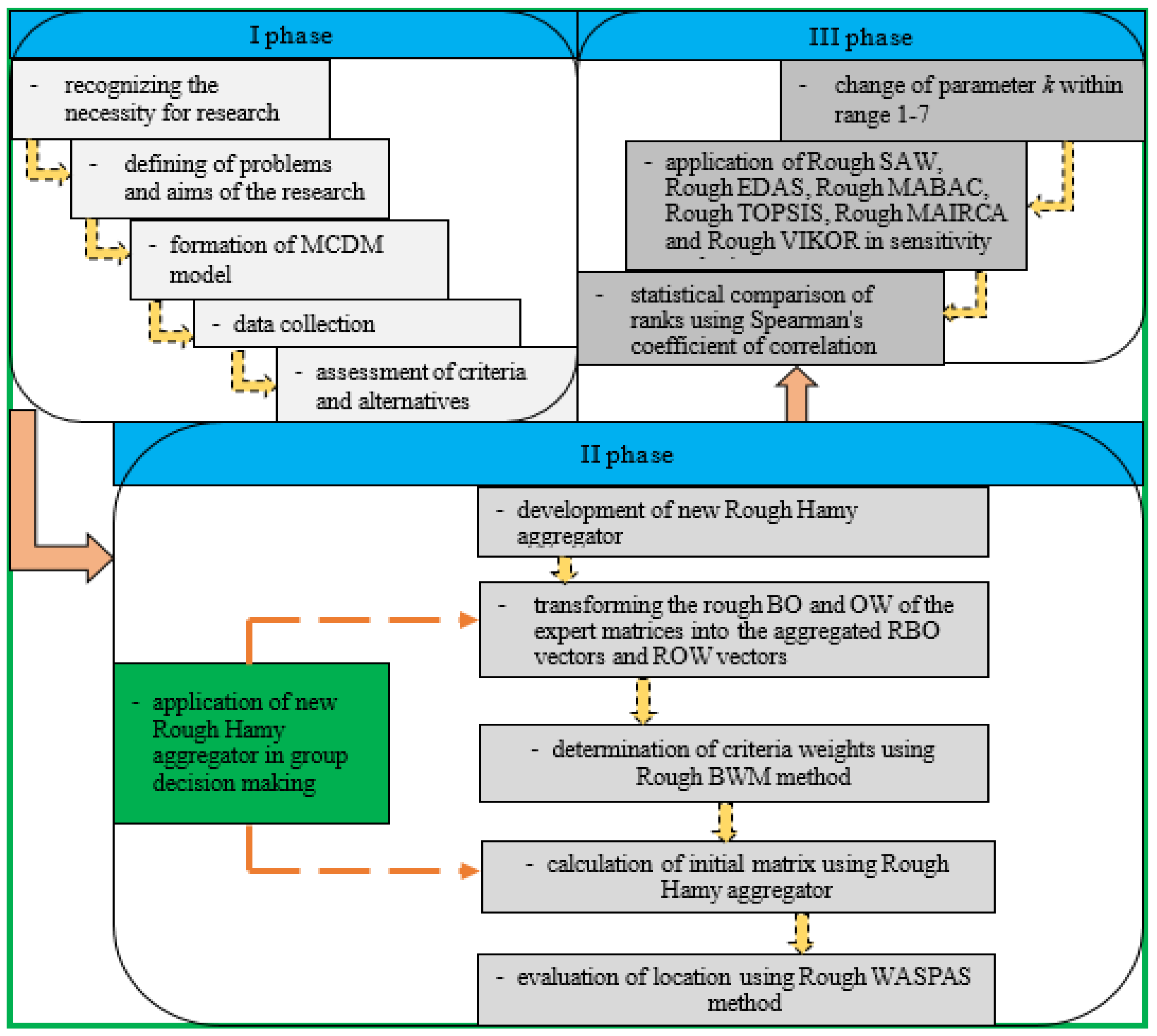
3.1. Proposed Methodology
3.2. Novel Rough Hamy Mean Operators and Their Operations
- (i).
- (ii).
- (iii).
4. The Location Selection for Roundabout Construction in Doboj
4.1. Forming a Multi-Criteria Model
4.2. Data Collection
4.3. Criteria Weight Calculation Using Rough BWM
4.4. Aggregation of an Initial Matrix on the Basis of the Developed Rough Hamy Aggregator
- (a)
- (b)
- (c)
4.5. Evaluation of Locations Using Rough WASPAS Methods
5. Sensitivity Analysis
6. Conclusions
Author Contributions
Funding
Conflicts of Interest
Appendix A
- (1)
- ,
- (2)
- ,
- (3)
- ,
- (4)
- .
- (1)
- If and , then it is obtained that ;
- (2)
- If and , then it can be concluded that there are the following equalities:
References
- Brown, M. The Design of Roundabouts; TRL State of the Art Review; Her Majesty Stationary Office: London, UK, 1995. [Google Scholar]
- Hels, T.; Orozova-Bekkevold, I. The effect of roundabout design features on cyclist accident rate. Accid. Anal. Prev. 2007, 39, 300–307. [Google Scholar] [CrossRef] [PubMed]
- Vasilyeva, E.; Sazonova, T. Justification of the Expediency of Creating Circular Intersections in Modern Cities. Earth Environ. Sci. 2017, 90, 012116. [Google Scholar] [CrossRef] [Green Version]
- Mottaeva, A. Innovative Aspects of Ecological and Economic Management of Investment and Construction Activities for the Sustainable Development of the Region. MATEC Web Conf. 2016, 73, 07020. [Google Scholar] [CrossRef] [Green Version]
- Møller, М.; Hels, Т. Cyclists’ perception of risk in roundabouts. Accid. Anal. Prev. 2008, 40, 1055–1062. [Google Scholar] [CrossRef] [PubMed]
- Li, Y.; Zhao, L.; Suo, J. Comprehensive assessment on sustainable development of highway transportation capacity based on entropy weight and TOPSIS. Sustainability 2014, 6, 4685–4693. [Google Scholar] [CrossRef]
- Pratelli, A. Design of modern roundabouts in urban traffic systems. WIT Trans. Built Environ. 2006, 89, 11. [Google Scholar]
- Retting, R.A.; Mandavilli, S.; McCartt, A.T.; Russell, E.R. Roundabouts, traffic flow and public opinion. Traffic Eng. Control 2006, 47, 268–272. [Google Scholar]
- Pratelli, A.; Sechi, P.; Roy Souleyrette, R. Upgrading Traffic Circles to Modern Roundabouts to Improve Safety and Efficiency–Case Studies from Italy. Promet-Traffic Transp. 2018, 30, 217–229. [Google Scholar] [CrossRef]
- Antov, D.; Abel, K.; Sürje, P.; Rouk, H.; Roivas, T. Speed reduction effects of urban roundabouts. Balt. J. Road Bridge Eng. 2009, 4. [Google Scholar] [CrossRef]
- Sohn, K. A systematic decision criterion for the elimination of useless overpasses. Transp. Res. Part A Policy Pract. 2008, 42, 1043–1055. [Google Scholar] [CrossRef]
- Podvezko, V.; Sivilevičius, H. The use of AHP and rank correlation methods for determining the significance of the interaction between the elements of a transport system having a strong influence on traffic safety. Transport 2013, 28, 389–403. [Google Scholar] [CrossRef]
- Pilko, H.; Mandžuka, S.; Barić, D. Urban single-lane roundabouts: A new analytical approach using multi-criteria and simultaneous multi-objective optimization of geometry design, efficiency and safety. Transp. Res. Part C Emerg. Technol. 2017, 80, 257–271. [Google Scholar] [CrossRef]
- Barić, D.; Pilko, H.; Strujić, J. An analytic hierarchy process model to evaluate road section design. Transport 2016, 31, 312–321. [Google Scholar] [CrossRef]
- Singh, T.P.; Nigam, S.P.; Singh, D.G.; Agrawal, V.P. Analysis and Validation of Traffic Noise under Dynamic Condition Near Roundabout Using Madm Approach. Ph.D. Thesis, LM Thapar School of Management, Behra, India, 2013. [Google Scholar]
- Pirdavani, A.; Brijs, T.; Wets, G. A Multiple Criteria Decision-Making Approach for Prioritizing Accident Hotspots in the Absence of Crash Data. Transp. Rev. 2010, 30, 97–113. [Google Scholar] [CrossRef]
- Murat, Y.S.; Arslan, T.; Cakici, Z.; Akçam, C. Analytical Hierarchy Process (AHP) based Decision Support System for Urban Intersections in Transportation Planning. In Using Decision Support Systems for Transportation Planning Efficiency; IGI Global: Hershey, PA, USA, 2016; pp. 203–222. [Google Scholar]
- Legac, I.; Pilko, H.; Brcic, D. Analysis of traffic capacity and design for the reconstruction of a large roundabout in the city of Zagreb. Intersec. Control Saf. 2013, 66, 17. [Google Scholar]
- Ruiz-Padillo, A.; Ruiz, D.P.; Torija, A.J.; Ramos-Ridao, Á. Selection of suitable alternatives to reduce the environmental impact of road traffic noise using a fuzzy multi-criteria decision model. Environ. Impact Assess. Rev. 2016, 61, 8–18. [Google Scholar] [CrossRef] [Green Version]
- Ruiz-Padillo, A.; Torija, A.J.; Ramos-Ridao, A.F.; Ruiz, D.P. Application of the fuzzy analytic hierarchy process in multi-criteria decision in noise action plans: Prioritizing road stretches. Environ. Model. Softw. 2016, 81, 45–55. [Google Scholar] [CrossRef] [Green Version]
- Joo, S.; Lee, G.; Oh, C. A multi-criteria analysis framework including environmental and health impacts for evaluating traffic calming measures at the road network level. Int. J. Sustain. Transp. 2017, 1–9. [Google Scholar] [CrossRef]
- Hao, N.; Feng, Y.; Zhang, K.; Tian, G.; Zhang, L.; Jia, H. Evaluation of traffic congestion degree: An integrated approach. Int. J. Distrib. Sens. Netw. 2017, 13. [Google Scholar] [CrossRef] [Green Version]
- Bongo, M.F.; Ocampo, L.A. A hybrid fuzzy MCDM approach for mitigating airport congestion: A case in Ninoy Aquino International Airport. J. Air Transp. Manag. 2017, 63, 1–16. [Google Scholar] [CrossRef]
- Hashemkhani Zolfani, S.; Esfahani, M.H.; Bitarafan, M.; Zavadskas, E.K.; Arefi, S.L. Developing a new hybrid MCDM method for selection of the optimal alternative of mechanical longitudinal ventilation of tunnel pollutants during automobile accidents. Transport 2013, 28, 89–96. [Google Scholar] [CrossRef]
- Castro-Nuño, M.; Arévalo-Quijada, M.T. Assessing urban road safety through multidimensional indexes: Application of multicriteria decision making analysis to rank the Spanish provinces. Transp. Policy 2018, 68, 118–129. [Google Scholar] [CrossRef]
- Gardziejczyk, W.; Zabicki, P. Normalization and variant assessment methods in selection of road alignment variants–case study. J. Civ. Eng. Manag. 2017, 23, 510–523. [Google Scholar] [CrossRef]
- Javid, R.J.; Nejat, A.; Hayhoe, K. Selection of CO2 mitigation strategies for road transportation in the United States using a multi-criteria approach. Renew. Sustain. Energy Rev. 2014, 38, 960–972. [Google Scholar] [CrossRef]
- Drezner, Z. Facility Location: A Survey of Applications and Methods; Springer: New York, NY, USA, 1995. [Google Scholar]
- Kahraman, C.; Ruan, D.; Doǧan, I. Fuzzy group decision-making for facility location selection. Inf. Sci. 2003, 157, 135–153. [Google Scholar] [CrossRef]
- Berman, O.; Drezner, Z.; Wesolowsky, G.O. Location of facilities on a network with groups of demand points. IIE Trans. 2001, 33, 637–648. [Google Scholar] [CrossRef]
- Melkote, S.; Daskin, M.S. Capacitated facility location/network design problems. Eur. J. Oper. Res. 2001, 129, 481–495. [Google Scholar] [CrossRef]
- Nanthavanij, S.; Yenradee, P. Predicting the optimum number, location, and signal sound level of auditory warning devices for manufacturing facilities. Int. J. Ind. Ergon. 1999, 24, 569–578. [Google Scholar] [CrossRef]
- Badri, M.A. Combining the analytic hierarchy process and goal programming for global facility location-allocation problem. Int. J. Prod. Econ. 1999, 62, 237–248. [Google Scholar] [CrossRef]
- Applebaum, W. The analog method for estimating potential store sales. Guid. Stor. Locat. Res. 1968, 3, 127–144. [Google Scholar]
- Stević, Ž.; Vesković, S.; Vasiljević, M.; Tepić, G. The selection of the logistics center location using AHP method. In Proceedings of the 2nd Logistics International Conference, Belgrade, Serbia, 21–23 May 2015; pp. 86–91. [Google Scholar]
- Benjamin, C.O.; Chi, S.C.; Gaber, T.; Riordan, C.A. Comparing BP and ART II neural network classifiers for facility location. Comput. Ind. Eng. 1995, 28, 43–50. [Google Scholar] [CrossRef]
- Satani, N.; Uchida, A.; Deguchi, A.; Ohgai, A.; Sato, S.; Hagishima, S. Commercial facility location model using multiple regression analysis. Comput. Environ. Urban Syst. 1998, 22, 219–240. [Google Scholar] [CrossRef]
- Chauhan, A.; Singh, A. A hybrid multi-criteria decision making method approach for selecting a sustainable location of healthcare waste disposal facility. J. Clean. Prod. 2016, 139, 1001–1010. [Google Scholar] [CrossRef]
- Nie, R.X.; Wang, J.Q.; Zhang, H.Y. Solving solar-wind power station location problem using an extended weighted aggregated sum product assessment (WASPAS) technique with interval neutrosophic sets. Symmetry 2017, 9, 106. [Google Scholar] [CrossRef]
- Samanlioglu, F.; Ayağ, Z. A fuzzy AHP-PROMETHEE II approach for evaluation of solar power plant location alternatives in Turkey. J. Intell. Fuzzy Syst. 2017, 33, 859–871. [Google Scholar] [CrossRef]
- Zhao, L.; Li, H.; Li, M.; Sun, Y.; Hu, Q.; Mao, S.; Li, J.; Xue, J. Location selection of intra-city distribution hubs in the metro-integrated logistics system. Tunn. Undergr. Space Technol. 2018, 80, 246–256. [Google Scholar] [CrossRef]
- Nazari, M.A.; Aslani, A.; Ghasempour, R. Analysis of solar farm site selection based on TOPSIS approach. Int. J. Soc. Ecol. Sustain. Dev. 2018, 9, 12–25. [Google Scholar] [CrossRef]
- Baušys, R.; Juodagalvienė, B. Garage location selection for residential house by WASPAS-SVNS method. J. Civ. Eng. Manag. 2017, 23, 421–429. [Google Scholar] [CrossRef]
- Pamučar, D.; Stević, Ž.; Zavadskas, E.K. Integration of interval rough AHP and interval rough MABAC methods for evaluating university web pages. Appl. Soft Comput. 2018, 67, 141–163. [Google Scholar] [CrossRef]
- Saaty, T.L.; Tran, L.T. On the invalidity of fuzzifying numerical judgments in the Analytic Hierarchy Process. Math. Comput. Model. 2007, 46, 962–975. [Google Scholar] [CrossRef]
- Wang, Y.M.; Luo, Y.; Hua, Z. On the extent analysis method for fuzzy AHP and its applications. Eur. J. Oper. Res. 2008, 186, 735–747. [Google Scholar] [CrossRef]
- Stević, Ž.; Pamučar, D.; Vasiljević, M.; Stojić, G.; Korica, S. Novel Integrated Multi-Criteria Model for Supplier Selection: Case Study Construction Company. Symmetry 2017, 9, 279. [Google Scholar] [CrossRef]
- Yager, R.R. On generalized Bonferroni mean operators for multi-criteria aggregation. Int. J. Approx. Reason. 2009, 50, 1279–1286. [Google Scholar] [CrossRef]
- Petrović, G.S.; Madić, M.; Antucheviciene, J. An approach for robust decision making rule generation: Solving transport and logistics decision making problems. Expert Syst. Appl. 2018, 106, 263–276. [Google Scholar] [CrossRef]
- Stefanovic-Marinovic, J.; Troha, S.; Milovančevic, M. An Application of Multicriteria Optimization to the Two-Carrier Two-Speed Planetary Gear Trains. Facta Univ. Ser. Mech. Eng. 2017, 15, 85–95. [Google Scholar] [CrossRef]
- Chatterjee, P.; Mondal, S.; Boral, S.; Banerjee, A.; Chakraborty, S. A novel hybrid method for non-traditional machining process selection using factor relationship and multi-attributive border approximation method. Facta Univ. Ser. Mech. Eng. 2017, 15, 439–456. [Google Scholar] [CrossRef]
- Rezaei, J. Best-worst multi-criteria decision-making method. Omega 2015, 53, 49–57. [Google Scholar] [CrossRef]
- Pamučar, D.; Gigović, L.; Bajić, Z.; Janošević, M. Location selection for wind farms using GIS multi-criteria hybrid model: An approach based on fuzzy and rough numbers. Sustainability 2017, 9, 1315. [Google Scholar] [CrossRef]
- Stević, Ž.; Pamučar, D.; Zavadskas, E.K.; Ćirović, G.; Prentkovskis, O. The Selection of Wagons for the Internal Transport of a Logistics Company: A Novel Approach Based on Rough BWM and Rough SAW Methods. Symmetry 2017, 9, 264. [Google Scholar] [CrossRef]
- Pamučar, D.; Petrović, I.; Ćirović, G. Modification of the Best–Worst and MABAC methods: A novel approach based on interval-valued fuzzy-rough numbers. Expert Syst. Appl. 2018, 91, 89–106. [Google Scholar] [CrossRef]
- Pawlak, Z. Rough Sets: Theoretical Aspects of Reasoning about Data; Springer: Berlin, Germany, 1991. [Google Scholar]
- Pawlak, Z. Anatomy of conflicts. Bull. Eur. Assoc. Theor. Comput. Sci. 1993, 50, 234–247. [Google Scholar]
- Stojić, G.; Stević, Ž.; Antuchevičienė, J.; Pamučar, D.; Vasiljević, M. A Novel Rough WASPAS Approach for Supplier Selection in a Company Manufacturing PVC Carpentry Products. Information 2018, 9, 121. [Google Scholar] [CrossRef]
- Hashemkhani Zolfani, S.; Aghdaie, M.H.; Derakhti, A.; Zavadskas, E.K.; Varzandeh, M.H.M. Decision making on business issues with foresight perspective; an application of new hybrid MCDM model in shopping mall locating. Expert Syst. Appl. 2013, 40, 7111–7121. [Google Scholar] [CrossRef]
- Mardani, A.; Nilashi, M.; Zavadskas, E.K.; Awang, S.R.; Zare, H.; Jamal, N.M. Decision making methods based on fuzzy aggregation operators: Three decades review from 1986 to 2017. Int. J. Inf. Technol. Decis. Mak. 2018, 17, 391–466. [Google Scholar] [CrossRef]
- Božanić, D.; Tešić, D.; Milićević, J. A hybrid fuzzy AHP-MABAC model: Application in the Serbian Army—The selection of the location for deep wading as a technique of crossing the river by tanks. Decis. Mak. Appl. Manag. Eng. 2018, 1, 143–164. [Google Scholar] [CrossRef]
- Roy, J.; Adhikary, K.; Kar, S.; Pamučar, D. A rough strength relational DEMATEL model for analysing the key success factors of hospital service quality. Decis. Mak. Appl. Manag. Eng. 2018, 1, 121–142. [Google Scholar] [CrossRef]
- Vasiljevic, M.; Fazlollahtabar, H.; Stevic, Z.; Veskovic, S. A rough multicriteria approach for evaluation of the supplier criteria in automotive industry. Decis. Mak. Appl. Manag. Eng. 2018, 1, 82–96. [Google Scholar] [CrossRef]
- Hara, T.; Uchiyama, M.; Takahasi, S.E. A refinement of various mean inequalities. J. Inequal. Appl. 1998, 2, 387–395. [Google Scholar] [CrossRef]
- Day, C.M.; Hainen, A.M.; Bullock, D.M. Best Practices for Roundabouts on State Highways; Publication Joint Transportation Research Program, Indiana Department of Transportation and Purdue University: West Lafayette, Indiana, 2013. [Google Scholar]
- Benekohal, R.F.; Atluri, V. Roundabout Evaluation and Design: A Site Selection Procedure; Illinois Center for Transportation (ICT): Rantoul, IL, USA, 2009. [Google Scholar]
- Deluka-Tibljaš, A.; Babić, S.; Cuculić, M.; Šurdonja, S. Possible reconstructions of intersections in urban areas by using roundabouts. In Proceedings of the The First International Conference on Road and Rail Infrastructure (CETRA 2010), Road and Rail Infrastructure, Opatija, Croatia, 17–18 May 2010; pp. 171–178. [Google Scholar]
- Steiner, R.L.; Washburn, S.; Elefteriadou, L.; Gan, A.; Alluri, P.; Michalaka, D.; Xu, R.; Rachmat, S.; Lytle, B.; Cavaretta, A. Roundabouts and Access Management; State of Florida Department of Transportation: Florida, FL, USA, 2014.
- Kozić, M.; Šurdonja, S.; Deluka-Tibljaš, A.; Karleuša, B.; Cuculić, M. Criteria for urban traffic infrastructure analyses–case study of implementation of Croatian Guidelines for Rounabouts on State Roads. In Proceedings of the 4th International Conference on Road and Rail Infrastructure, Šibenik, Croatia, 23–25 May 2016. [Google Scholar]
- Retting, R.; Kyrychenko, S.; McCartt, A. Long-term trends in public opinion following construction of roundabouts. Transp. Res. Rec. J. Transp. Res. Board 2007, 2019, 219–224. [Google Scholar] [CrossRef]
- Zavadskas, E.K.; Stević, Ž.; Tanackov, I.; Prentkovskis, O. A Novel Multicriteria Approach–Rough Step-Wise Weight Assessment Ratio Analysis Method (R-SWARA) and Its Application in Logistics. Stud. Inf. Control 2018, 27, 97–106. [Google Scholar] [CrossRef]
- Qin, J. Interval type-2 fuzzy Hamy mean operators and their application in multiple criteria decision making. Granul. Comput. 2017, 2, 249–269. [Google Scholar] [CrossRef]
- Liu, P.; You, X. Some linguistic neutrosophic Hamy mean operators and their application to multi-attribute group decision making. PLoS ONE 2018, 13, e0193027. [Google Scholar] [CrossRef] [PubMed]
- Roy, J.; Chatterjee, K.; Bandhopadhyay, A.; Kar, S. Evaluation and selection of Medical Tourism sites: A rough AHP based MABAC approach. arXiv, 2016; arXiv:1606.08962. [Google Scholar]
- Song, W.; Ming, X.; Wu, Z.; Zhu, B. A rough TOPSIS approach for failure mode and effects analysis in uncertain environments. Qual. Reliab. Eng. Int. 2014, 30, 473–486. [Google Scholar] [CrossRef]
- Pamučar, D.; Mihajlović, M.; Obradović, R.; Atanasković, P. Novel approach to group multi-criteria decision making based on interval rough numbers: Hybrid DEMATEL-ANP-MAIRCA model. Expert Syst. Appl. 2017, 88, 58–80. [Google Scholar] [CrossRef]
- Zhu, G.N.; Hu, J.; Qi, J.; Gu, C.C.; Peng, Y.H. An integrated AHP and VIKOR for design concept evaluation based on rough number. Adv. Eng. Inf. 2015, 29, 408–418. [Google Scholar] [CrossRef]
- Keshavarz Ghorabaee, M.; Zavadskas, E.K.; Turskis, Z.; Antucheviciene, J. A new combinative distance-based assessment (CODAS) method for multi-criteria decision-making. Econ. Comput. Econ. Cybern. Stud. Res. 2016, 50, 25–44. [Google Scholar]


| Ref. | Approach | Purpose of Application |
|---|---|---|
| [11] | AHP | elimination of unnecessary overpasses that had lost their positive function in the traffic flow |
| [12] | AHP | determination of the influence of traffic factor interaction on the rate of traffic accidents |
| [13] | MOO and AHP | evaluation and ranking traffic and geometric elements |
| [14] | AHP | evaluation of road section design in an urban environment |
| [15] | TOPSIS | evaluation of locations with roundabouts and noise analysis in them |
| [16] | Delphi and TOPSIS | identification of priority black spots in order to increase the safety in traffic |
| [17] | AHP | evaluation of four types of intersections |
| [18] | AHP | evaluation of variants for roundabout reconstruction |
| [19] | Fuzzy AHP, WSM ELECTRE and TOPSIS | evaluation of the alternatives for noise reduction in traffic |
| [20] | Fuzzy AHP | prioritizing road stretches included in a noise action plans |
| [21] | AHP | evaluation of the effectiveness of traffic calming measures |
| [22] | Fuzzy AHP and TOPSIS | evaluation of traffic congestion rates |
| [23] | ANP, DEMATEL, fuzzy set theory and TOPSIS | mitigation of congestion at the Ninoy Aquino airport |
| [24] | SWARA and VIKOR | selection of the optimal alternative of mechanical longitudinal ventilation of tunnel pollutants during automobile accidents |
| [25] | PROMETHEE | determination of urban road safety |
| [27] | AHP | ranking various on-road emission mitigation strategies |
| [39] | WASPAS with interval neutrosophic sets | the solar-wind power station location selection |
| [40] | Fuzzy AHP and Fuzzy PROMETHEE II | selection the best location for a solar power plant |
| [41] | AHP and TOPSIS | construction of a metro-integrated logistics system |
| [42] | TOPSIS | selection of suitable site for photovoltaic installation |
| [43] | WASPAS with single-valued neutrosophic sets | determination of the location problem of a garage for a residential house |
| Ord. No. | Criterion | Criterion Description |
|---|---|---|
| 1 | Flow of vehicles | The number of vehicles passing through the observed road intersection in a unit of time in both directions. |
| 2 | Flow of pedestrians | The number of pedestrians crossing the observed intersection at the point for pedestrian movement (pedestrian crossing, zebra, etc.) at a given time interval. |
| 3 | Traffic safety indicator | The number of traffic accidents on the observed section of the road |
| 4 | Costs of construction and exploitation | Cost estimation (construction, exploitation and maintenance) |
| 5 | Type of intersection | Three-way or four-way intersections |
| 6 | Average vehicle intensity per access arm | The limit intensity is the intensity at the entry arm into the intersection of 360 PA/h |
| 7 | Functional criterion of spatial fitting | What is the primary role of the intersection observed? This section analyzes what type of intersection is the most acceptable due to its role in traffic. |
| 8 | Public opinion | It implies a survey of local population that have chosen one of the offered locations as a priority for the construction of a roundabout. |
| C1 | C2 | C3 | C4 | C5 | C6 | C7 | C8 | |
|---|---|---|---|---|---|---|---|---|
| A1 | 1256 | 8 | 2 | 3 | 3 | 419 | 7 | 85 |
| A2 | 2194 | 4 | 2 | 9 | 3 | 731 | 5 | 89 |
| A3 | 1037 | 5 | 4 | 7 | 3 | 346 | 3 | 45 |
| A4 | 2878 | 32 | 3 | 7 | 4 | 720 | 5 | 8 |
| A5 | 1052 | 2 | 4 | 5 | 4 | 263 | 5 | 27 |
| A6 | 4197 | 124 | 1 | 3 | 4 | 1050 | 7 | 74 |
| Location 1—Exit from the Old Town onto the M17 Main Road | |||||||||||||
| Direction | Bare-Maglaj | Bare-Old Town | Maglaj-Bare | Maglaj-Old Town | Old Town-Bare | Old Town-Maglaj | Ʃ | ||||||
| Trucks | 64 | 12 | 64 | 12 | 12 | 24 | 176 | ||||||
| Passenger vehicles | 268 | 84 | 388 | 108 | 160 | 72 | 1080 | ||||||
| Location 2—The Bridge, So-Called “Japanac”, Which Represents the Entrance into the Town from Tuzla | |||||||||||||
| Direction | “Japanac”-Maglaj | “Japanac“-Bare | Maglaj-“Japanac” | Maglaj-Bare | Bare-Maglaj | Bare-“Japanac” | Ʃ | ||||||
| Trucks | 60 | 52 | 72 | 84 | 112 | 80 | 462 | ||||||
| Passenger vehicles | 200 | 240 | 360 | 380 | 272 | 280 | 1732 | ||||||
| Location 3—The Intersection on the M17 Main Road at Flea Market | |||||||||||||
| Direction | Bare-Maglaj | Bare-Town Entrance | Maglaj-Bare | Maglaj-Town Entrance | Town Exit-Bare | Town Exit-Maglaj | Ʃ | ||||||
| Trucks | 76 | 0 | 80 | 0 | 0 | 0 | 156 | ||||||
| Passenger vehicles | 244 | 108 | 384 | 24 | 100 | 24 | 884 | ||||||
| Location 4—Traffic-Light Intersection on the M17 Main Road | |||||||||||||
| Direction | Town-Railwaysstation | Town-Maglaj | Town-Bare | Bare-Maglaj | Bare-Town | Bare-r. Stat. | Maglaj-Bare | Mag.-Town | Mag.-r. Station | R. stat.-Bare | R. Stat.-Maglaj | R. Stat.-Town | Ʃ |
| Trucks | 9 | 15 | 24 | 90 | 15 | 27 | 96 | 27 | 24 | 30 | 25 | 15 | 397 |
| Passenger vehicles | 153 | 225 | 240 | 270 | 105 | 135 | 300 | 270 | 120 | 132 | 246 | 285 | 2481 |
| Location 5—Intersection at the Entrance into/Exit from the Town via Usora | |||||||||||||
| Direction | Bare-Maglaj | Bare-Usora | Maglaj-Bare | Maglaj-Usora | Usora-Bare | Usora-Maglaj | Ʃ | ||||||
| Trucks | 68 | 0 | 100 | 4 | 0 | 4 | 176 | ||||||
| Passenger vehicles | 232 | 140 | 288 | 152 | 24 | 40 | 876 | ||||||
| Location 6—Intersection in the Town at the Junction of Jug Bogdana and Cara Dušana Street | |||||||||||||
| Direction | Church-Vladimirka | Church-Center | Church-Bingo | Vlad.-Church | Vlad.-Center | Vlad.-Bingo | Center-Church | Center-Vlad. | Center-Bingo | Bingo.-Center | Bingo-Church | Bingo-Vlad. | Ʃ |
| Trucks | 9 | 15 | 24 | 90 | 15 | 27 | 96 | 27 | 24 | 30 | 25 | 15 | 397 |
| Passenger vehicles | 569 | 292 | 478 | 507 | 139 | 234 | 222 | 129 | 374 | 403 | 365 | 88 | 3800 |
| BO | OW | |||||||||||||
|---|---|---|---|---|---|---|---|---|---|---|---|---|---|---|
| Criteria | E1 | E2 | E3 | E4 | E5 | E6 | E7 | E1 | E2 | E3 | E4 | E5 | E6 | E7 |
| C1 | 1 | 1 | 2 | 1 | 1 | 1 | 1 | 6 | 6 | 4 | 6 | 8 | 7 | 7 |
| C2 | 2 | 3 | 3 | 4 | 4 | 1 | 2 | 5 | 4 | 3 | 3 | 3 | 6 | 5 |
| C3 | 1 | 2 | 1 | 2 | 2 | 1 | 1 | 6 | 5 | 5 | 5 | 5 | 6 | 6 |
| C4 | 3 | 4 | 4 | 3 | 3 | 4 | 5 | 3 | 3 | 2 | 4 | 4 | 3 | 2 |
| C5 | 2 | 3 | 3 | 3 | 5 | 2 | 2 | 4 | 4 | 3 | 4 | 2 | 5 | 5 |
| C6 | 4 | 5 | 4 | 4 | 6 | 1 | 5 | 2 | 2 | 2 | 3 | 1 | 6 | 2 |
| C7 | 3 | 4 | 4 | 5 | 7 | 5 | 2 | 3 | 3 | 2 | 2 | 1 | 2 | 5 |
| C8 | 6 | 6 | 5 | 6 | 8 | 7 | 7 | 1 | 1 | 1 | 1 | 1 | 1 | 1 |
| BO | |||||||
| Criteria | E1 | E2 | E3 | E4 | E5 | E6 | E7 |
| C1 | [1, 1.14] | [1, 1.16] | [1.16, 2] | [1, 1.02] | [1, 1.04] | [1, 1.04] | [1, 1.04] |
| C2 | [1.67, 2.96] | [2.34, 3.5] | [2.08, 3.67] | [2.53, 4] | [2.26, 4] | [1, 2.05] | [1.84, 2.32] |
| C3 | [1, 1.43] | [1.49, 2] | [1, 1.35] | [1.42, 2] | [1.27, 2] | [1, 1.19] | [1, 1.23] |
| C4 | [3, 3.71] | [3.62, 4.25] | [3.45, 4.33] | [3, 3.62] | [3, 3.68] | [3.46, 4.5] | [3.54, 5] |
| C5 | [2, 2.86] | [2.64, 3.5] | [2.48, 3.67] | [2.42, 4] | [2.71, 5] | [2, 2.34] | [2, 2.44] |
| C6 | [3.25, 4.59] | [3.86, 5.33] | [3.06, 4.63] | [3.03, 4.79] | [3.76, 6] | [1, 3.33] | [3.73, 5] |
| C7 | [2.5, 4.61] | [3.33, 4.88] | [2.83, 5.06] | [3.69, 5.67] | [3.85, 7] | [3.38, 5] | [2, 3.21] |
| C8 | [5.75, 6.63] | [5.67, 6.74] | [5, 6.45] | [5.81, 6.89] | [6.41, 8] | [6.09, 7] | [6.01, 7] |
| OW | |||||||
| Criteria | E1 | E2 | E3 | E4 | E5 | E6 | E7 |
| C1 | [5.5, 6.61] | [5.33, 6.71] | [4, 6.26] | [5.61, 6.86] | [6.16, 8] | [5.82, 7] | [5.7, 7] |
| C2 | [3.88, 5.33] | [3.25, 4.79] | [3, 4] | [3, 4.04] | [3, 4.04] | [4.04, 6] | [3.61, 5] |
| C3 | [5.43, 6] | [5, 5.35] | [5, 5.41] | [5, 5.41] | [5, 5.41] | [5.41, 6] | [5.27, 6] |
| C4 | [2.67, 3.33] | [2.6, 3.4] | [2, 2.95] | [3.04, 4] | [2.75, 4] | [2.55, 3.01] | [2, 2.58] |
| C5 | [3.48, 4.4] | [3.37, 4,5] | [2.5, 4.06] | [3.34, 4.67] | [2, 3.6] | [3.79, 5] | [3.36, 5] |
| C6 | [1.8, 2.8] | [1.75, 2.93] | [1.7, 3.11] | [2.02, 4.5] | [1, 2.4] | [2.55, 6] | [1.65, 2.2] |
| C7 | [2.22, 3.67] | [2.1, 4] | [1.75, 2.63] | [1.67, 2.65] | [1, 2.38] | [1.81, 2.78] | [2.33, 5] |
| C8 | [1, 1] | [1, 1] | [1, 1] | [1, 1] | [1, 1] | [1, 1] | [1, 1] |
| Best: C1 | RN | Worst: C8 | RN |
|---|---|---|---|
| C1 | [1.02, 1.18] | C1 | [5.42, 6.91] |
| C2 | [2.10, 3.16] | C2 | [3.38, 4.71] |
| C3 | [1.41, 1.58] | C3 | [5.16, 5.65] |
| C4 | [3.33, 4.14] | C4 | [2.50, 3.30] |
| C5 | [2.78, 3.34] | C5 | [3.08, 4.45] |
| C6 | [3.10, 4.77] | C6 | [1.75, 3.30] |
| C7 | [3.58, 5.00] | C7 | [1.81, 3.24] |
| C8 | [6.13, 6.95] | C8 | [1.00, 1.00] |
| A1 | A2 | A3 | |||||||||||||||||||
| C1 | 3 | 3 | 5 | 3 | 3 | 3 | 1 | 5 | 5 | 7 | 5 | 5 | 5 | 3 | 1 | 1 | 3 | 3 | 3 | 3 | 1 |
| C2 | 5 | 3 | 3 | 3 | 3 | 3 | 1 | 3 | 1 | 3 | 1 | 3 | 1 | 1 | 3 | 1 | 3 | 3 | 3 | 1 | 1 |
| C3 | 5 | 3 | 1 | 5 | 3 | 3 | 3 | 5 | 3 | 1 | 5 | 3 | 3 | 3 | 9 | 7 | 5 | 9 | 7 | 5 | 7 |
| C4 | 5 | 3 | 5 | 3 | 1 | 3 | 3 | 7 | 1 | 7 | 5 | 5 | 7 | 9 | 5 | 1 | 5 | 3 | 3 | 7 | 7 |
| C5 | 7 | 5 | 7 | 7 | 5 | 7 | 5 | 7 | 5 | 7 | 7 | 5 | 7 | 5 | 7 | 5 | 7 | 7 | 5 | 7 | 5 |
| C6 | 5 | 5 | 3 | 5 | 3 | 5 | 3 | 7 | 7 | 5 | 7 | 5 | 7 | 5 | 3 | 5 | 1 | 5 | 3 | 3 | 1 |
| C7 | 7 | 7 | 9 | 7 | 9 | 7 | 7 | 9 | 9 | 7 | 7 | 7 | 7 | 5 | 5 | 7 | 5 | 5 | 7 | 7 | 3 |
| C8 | 9 | 7 | 9 | 7 | 9 | 7 | 9 | 9 | 7 | 9 | 7 | 9 | 7 | 9 | 5 | 5 | 5 | 5 | 5 | 5 | 5 |
| A4 | A5 | A6 | |||||||||||||||||||
| C1 | 7 | 5 | 7 | 5 | 5 | 5 | 5 | 1 | 1 | 3 | 3 | 3 | 3 | 1 | 9 | 7 | 9 | 7 | 9 | 7 | 7 |
| C2 | 7 | 7 | 5 | 5 | 7 | 5 | 5 | 1 | 1 | 1 | 1 | 1 | 1 | 1 | 9 | 9 | 7 | 9 | 9 | 9 | 9 |
| C3 | 7 | 5 | 3 | 7 | 5 | 3 | 5 | 9 | 7 | 5 | 9 | 7 | 5 | 7 | 1 | 1 | 1 | 3 | 1 | 1 | 1 |
| C4 | 5 | 3 | 7 | 5 | 3 | 3 | 7 | 3 | 1 | 3 | 5 | 3 | 3 | 5 | 5 | 1 | 3 | 3 | 3 | 1 | 3 |
| C5 | 9 | 7 | 9 | 9 | 7 | 9 | 7 | 9 | 7 | 9 | 9 | 7 | 9 | 7 | 9 | 7 | 9 | 9 | 7 | 9 | 7 |
| C6 | 7 | 7 | 5 | 7 | 5 | 7 | 5 | 1 | 3 | 1 | 3 | 3 | 1 | 1 | 9 | 9 | 7 | 9 | 9 | 9 | 7 |
| C7 | 5 | 7 | 5 | 3 | 3 | 7 | 5 | 7 | 7 | 7 | 5 | 5 | 9 | 5 | 5 | 9 | 5 | 7 | 7 | 7 | 7 |
| C8 | 1 | 3 | 1 | 1 | 1 | 1 | 1 | 3 | 3 | 3 | 5 | 3 | 5 | 3 | 7 | 7 | 7 | 5 | 7 | 5 | 7 |
| C1 | C2 | C3 | C4 | C5 | C6 | C7 | C8 | |
|---|---|---|---|---|---|---|---|---|
| A1 | [2.42, 3.49] | [2.42, 3.49] | [2.49, 3.97] | [2.49, 3.97] | [5.63, 6.62] | [3.63, 4.62] | [7.16, 7.96] | [7.64, 8.63] |
| A2 | [4.45, 5.5] | [1.33, 2.31] | [2.49, 3.97] | [4.07, 7.21] | [5.63, 6.62] | [5.63, 6.62] | [6.54, 7.98] | [7.64, 8.63] |
| A3 | [1.59, 2.61] | [1.59, 2.61] | [6.06, 7.89] | [2.89, 5.73] | [5.63, 6.62] | [1.99, 3.87] | [4.69, 6.35] | [5, 5] |
| A4 | [5.16, 5.96] | [5.36, 6.33] | [4.04, 5.89] | [3.68, 5.69] | [7.64, 8.63] | [5.63, 6.62] | [4.04, 5.89] | [1.04, 1.48] |
| A5 | [1.59, 2.61] | [1, 1] | [6.06, 7.89] | [2.49, 3.97] | [7.64, 8.63] | [1.33, 2.31] | [5.62, 7.23] | [3.16, 3.95] |
| A6 | [7.36, 8.34] | [8.45, 8.96] | [1.04, 1.48] | [1.93, 3.39] | [7.64, 8.63] | [8.01, 8.83] | [5.98, 7.41] | [6, 6.83] |
| C1 | C2 | C3 | C4 | C5 | C6 | C7 | C8 | |
|---|---|---|---|---|---|---|---|---|
| A1 | [0.29, 0.47] | [0.29, 0.41] | [0.32, 0.65] | [0.49, 1.36] | [0.65, 0.87] | [0.41, 0.58] | [0.9, 1.11] | [0.89, 1.13] |
| A2 | [0.53, 0.75] | [0.43, 0.75] | [0.32, 0.65] | [0.27, 0.83] | [0.65, 0.87] | [0.64, 0.83] | [0.82, 1.11] | [0.89, 1.13] |
| A3 | [0.19, 0.35] | [0.38, 0.63] | [0.77, 1.3] | [0.34, 1.17] | [0.65, 0.87] | [0.23, 0.48] | [0.59, 0.89] | [0.58, 0.65] |
| A4 | [0.62, 0.81] | [0.16, 0.19] | [0.51, 0.97] | [0.34, 0.92] | [0.89, 1.13] | [0.64, 0.83] | [0.51, 0.82] | [0.12, 0.19] |
| A5 | [0.19, 0.35] | [1, 1] | [0.77, 1.3] | [0.49, 1.36] | [0.89, 1.13] | [0.15, 0.29] | [0.7, 1.01] | [0.37, 0.52] |
| A6 | [0.88, 1.13] | [0.11, 0.12] | [0.13, 0.24] | [0.57, 1.76] | [0.89, 1.13] | [0.91, 1.1] | [0.75, 1.04] | [0.7, 0.89] |
| C1 | C2 | C3 | C4 | C5 | C6 | C7 | C8 | |
|---|---|---|---|---|---|---|---|---|
| A1 | [0.07, 0.14] | [0.04, 0.05] | [0.05, 0.11] | [0.03, 0.13] | [0.08, 0.10] | [0.02, 0.05] | [0.05, 0.08] | [0.03, 0.04] |
| A2 | [0.13, 0.22] | [0.06, 0.10] | [0.05, 0.11] | [0.01, 0.08] | [0.08, 0.10] | [0.04, 0.07] | [0.04, 0.09] | [0.03, 0.04] |
| A3 | [0.05, 0.10] | [0.05, 0.08] | [0.13, 0.21] | [0.02, 0.02] | [0.08, 0.10] | [0.01, 0.04] | [0.03, 0.07] | [0.02, 0.02] |
| A4 | [0.15, 0.24] | [0.02, 0.02] | [0.08, 0.16] | [0.02, 0.09] | [0.11, 0.14] | [0.04, 0.07] | [0.03, 0.06] | [0, 0.01] |
| A5 | [0.05, 0.10] | [0.13, 0.13] | [0.13, 0.21] | [0.03, 0.13] | [0.11, 0.14] | [0.01, 0.02] | [0.04, 0.08] | [0.01, 0.02] |
| A6 | [0.21, 0.33] | [0.01, 0.02] | [0.02, 0.04] | [0.03, 0.17] | [0.11, 0.14] | [0.05, 0.09] | [0.04, 0.08] | [0.03, 0.03] |
| Ai | Rank | |||
|---|---|---|---|---|
| A1 | [0.303, 0.891] | [−0.113, 0.113] | [0.189, 1.004] | 6 |
| A2 | [0.364, 1.007] | [−0.137, 0.137] | [0.227, 1.144] | 3 |
| A3 | [0.317, 0.940] | [−0.113, 0.115] | [0.205, 1.055] | 5 |
| A4 | [0.369, 0.983] | [−0.128, 0.119] | [0.240, 1.102] | 4 |
| A5 | [0.409, 1.050] | [−0.131, 0.123] | [0.278, 1.172] | 2 |
| A6 | [0.415, 1.124] | [−0.122, 0.116] | [0.293, 1.240] | 1 |
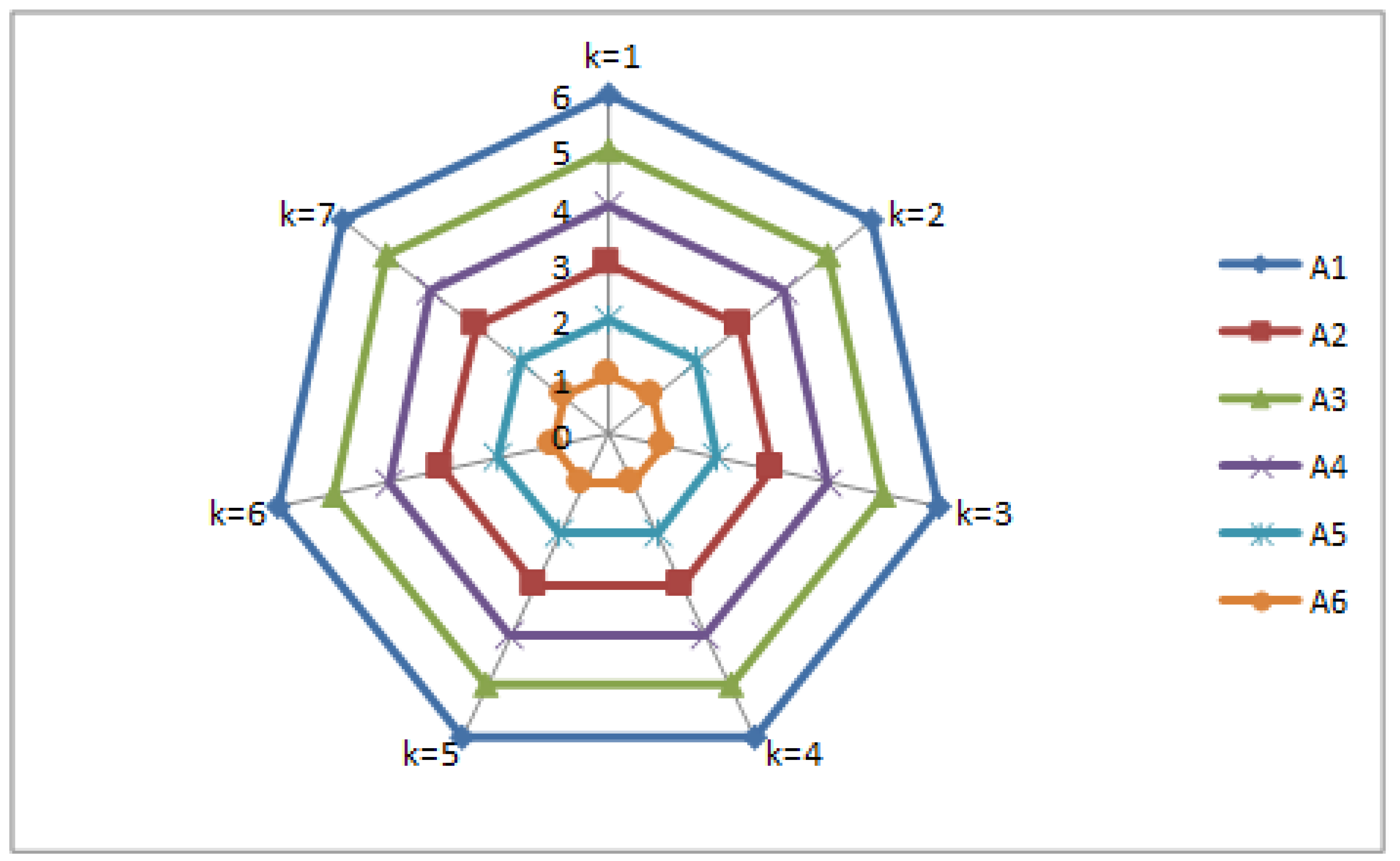
| Alte. | k = 1 | k = 2 | k = 3 | k = 4 | k = 5 | k = 6 | k = 7 |
|---|---|---|---|---|---|---|---|
| A1 | 0.595 | 0.597 | 0.599 | 0.669 | 0.679 | 0.681 | 0.682 |
| A2 | 0.702 | 0.686 | 0.685 | 0.739 | 0.746 | 0.747 | 0.748 |
| A3 | 0.638 | 0.630 | 0.631 | 0.694 | 0.703 | 0.704 | 0.705 |
| A4 | 0.684 | 0.671 | 0.669 | 0.718 | 0.726 | 0.727 | 0.728 |
| A5 | 0.734 | 0.725 | 0.726 | 0.749 | 0.754 | 0.755 | 0.756 |
| A6 | 0.767 | 0.766 | 0.768 | 0.774 | 0.778 | 0.778 | 0.779 |
| Ranking | A6 > A5 > A2 > A4 > A3 > A1 | A6 > A5 > A2 > A4 > A3 > A1 | A6 > A5 > A2 > A4 > A3 > A1 | A6 > A5 > A2 > A4 > A3 > A1 | A6 > A5 > A2 > A4 > A3 > A1 | A6 > A5 > A2 > A4 > A3 > A1 | A6 > A5 > A2 > A4 > A3 > A1 |
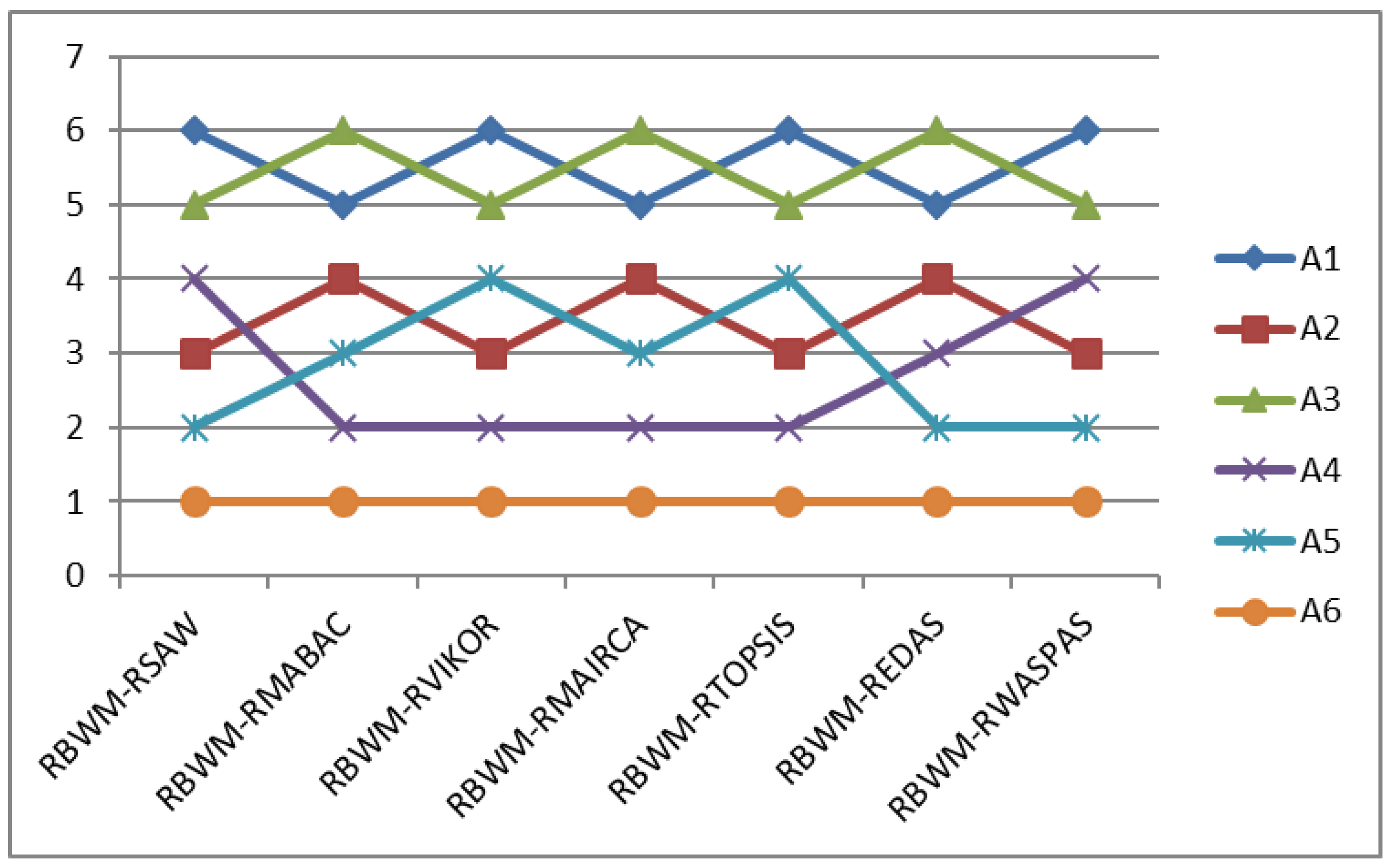
| Methods | RBWM-RWASPAS | RBWM-RSAW | RBWM-RMABAC | RBWM-RVIKOR | RBWM-RMAIRCA | RBWM-RTOPSIS | RBWM-REDAS | Average |
|---|---|---|---|---|---|---|---|---|
| RBWM-RWASPAS | 1.000 | 1.000 | 0.771 | 0.771 | 0.771 | 0.771 | 0.886 | 0.853 |
| RBWM-RSAW | - | 1.000 | 0.771 | 0.771 | 0.771 | 0.771 | 0.886 | 0.828 |
| RBWM-RMABAC | - | - | 1.000 | 0.886 | 1.000 | 0.886 | 0.943 | 0.943 |
| RBWM-RVIKOR | - | - | - | 1.000 | 0.886 | 1.000 | 0.771 | 0.914 |
| RBWM-RMAIRCA | - | - | - | - | 1.000 | 0.886 | 0.943 | 0.943 |
| RBWM-RTOPSIS | - | - | - | - | - | 1.000 | 0.771 | 0.886 |
| RBWM-REDAS | - | - | - | - | - | - | 1.000 | 1.000 |
| Overall average | 0.910 | |||||||
© 2018 by the authors. Licensee MDPI, Basel, Switzerland. This article is an open access article distributed under the terms and conditions of the Creative Commons Attribution (CC BY) license (http://creativecommons.org/licenses/by/4.0/).
Share and Cite
Stević, Ž.; Pamučar, D.; Subotić, M.; Antuchevičiene, J.; Zavadskas, E.K. The Location Selection for Roundabout Construction Using Rough BWM-Rough WASPAS Approach Based on a New Rough Hamy Aggregator. Sustainability 2018, 10, 2817. https://doi.org/10.3390/su10082817
Stević Ž, Pamučar D, Subotić M, Antuchevičiene J, Zavadskas EK. The Location Selection for Roundabout Construction Using Rough BWM-Rough WASPAS Approach Based on a New Rough Hamy Aggregator. Sustainability. 2018; 10(8):2817. https://doi.org/10.3390/su10082817
Chicago/Turabian StyleStević, Željko, Dragan Pamučar, Marko Subotić, Jurgita Antuchevičiene, and Edmundas Kazimieras Zavadskas. 2018. "The Location Selection for Roundabout Construction Using Rough BWM-Rough WASPAS Approach Based on a New Rough Hamy Aggregator" Sustainability 10, no. 8: 2817. https://doi.org/10.3390/su10082817