
Minimalist Deployment of Neural Network Equalizers in a Bandwidth-Limited Optical Wireless Communication System with Knowledge Distillation


Abstract
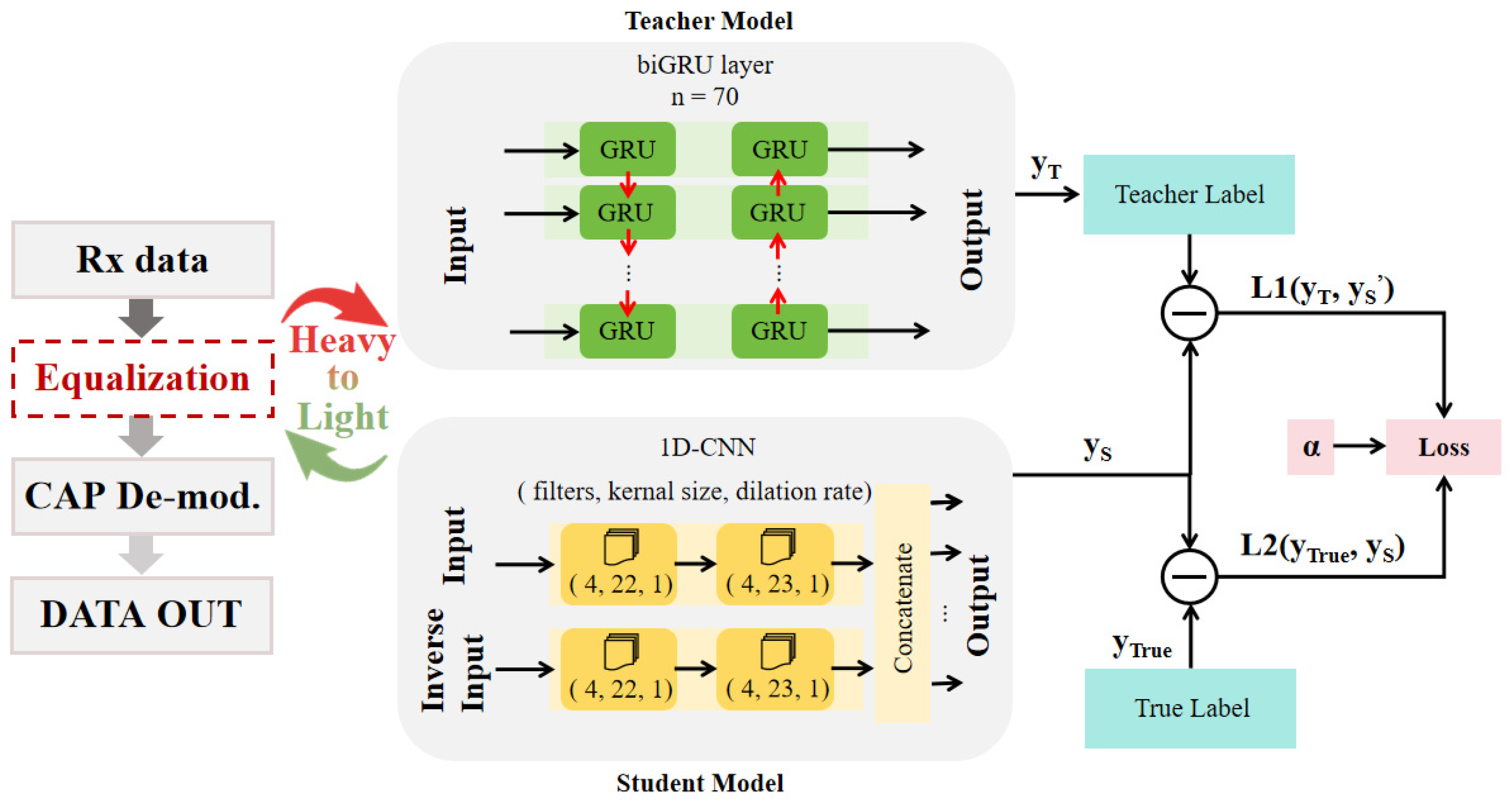
:1. Introduction
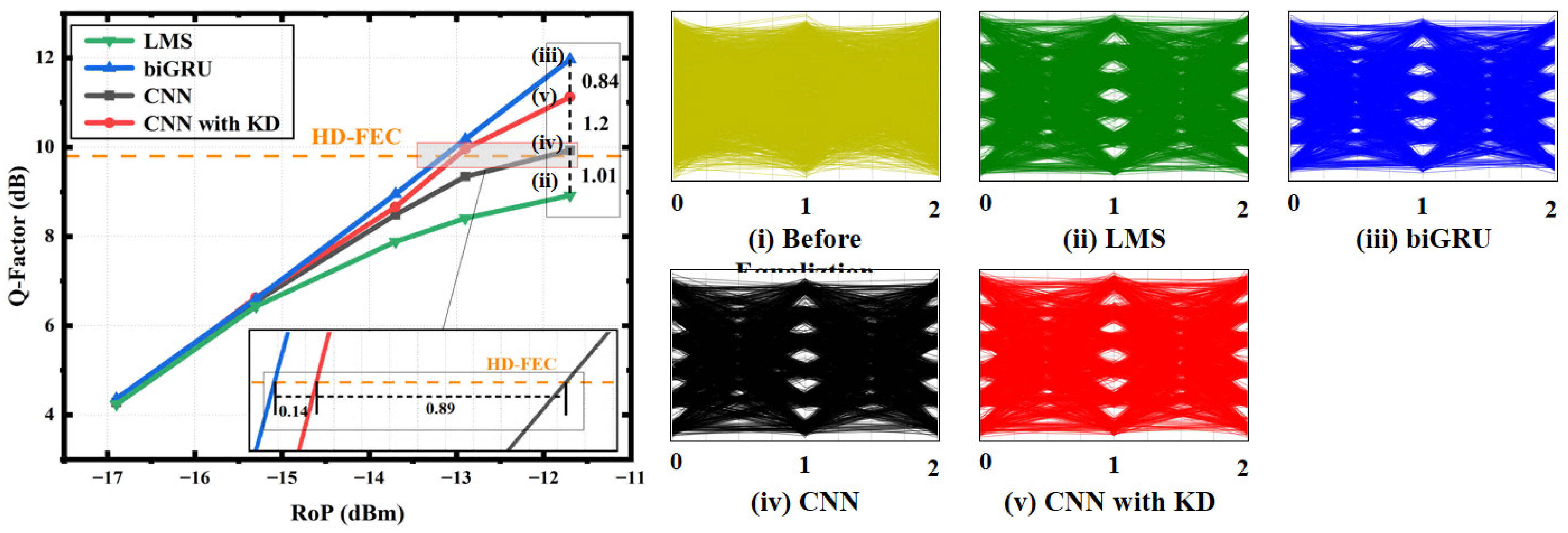
- We propose a solution using KD to distill the biGRU-based equalizer to obtain a network structure that can be parallelized. We transfer the knowledge that can recognize temporal signals from the teacher model based on the biGRU to the student model 1D-CNN, which can be processed in parallel, so that the student model also has the ability to recognize temporal information [10]. We compare the biGRU, 1D-CNN after KD and 1D-CNN without KD in terms of Q-factor and equalization velocity. The experimental data showed that the Q-factor of the 1D-CNN increased by 1 dB after KD learning from the biGRU, and KD increased the RoP sensitivity of the 1D-CNN by 0.89 dB on the HD-FEC threshold of 1 × 10⁻³.
- More importantly, we used the parallelization ability of the student model to achieve a huge speed increase: the proposed 1D-CNN reduces the computational time by 97% and the number of trainable parameters by 99.3% compared with the biGRU.
- Through experimentation, the effectiveness of the network after KD was tested in different situations with different parameters. The results demonstrate that the proposed minimalist 1D-CNN equalizer holds significant promise for future practical deployments in optical wireless communication systems.
2. Methods
2.1. Knowledge Distillation
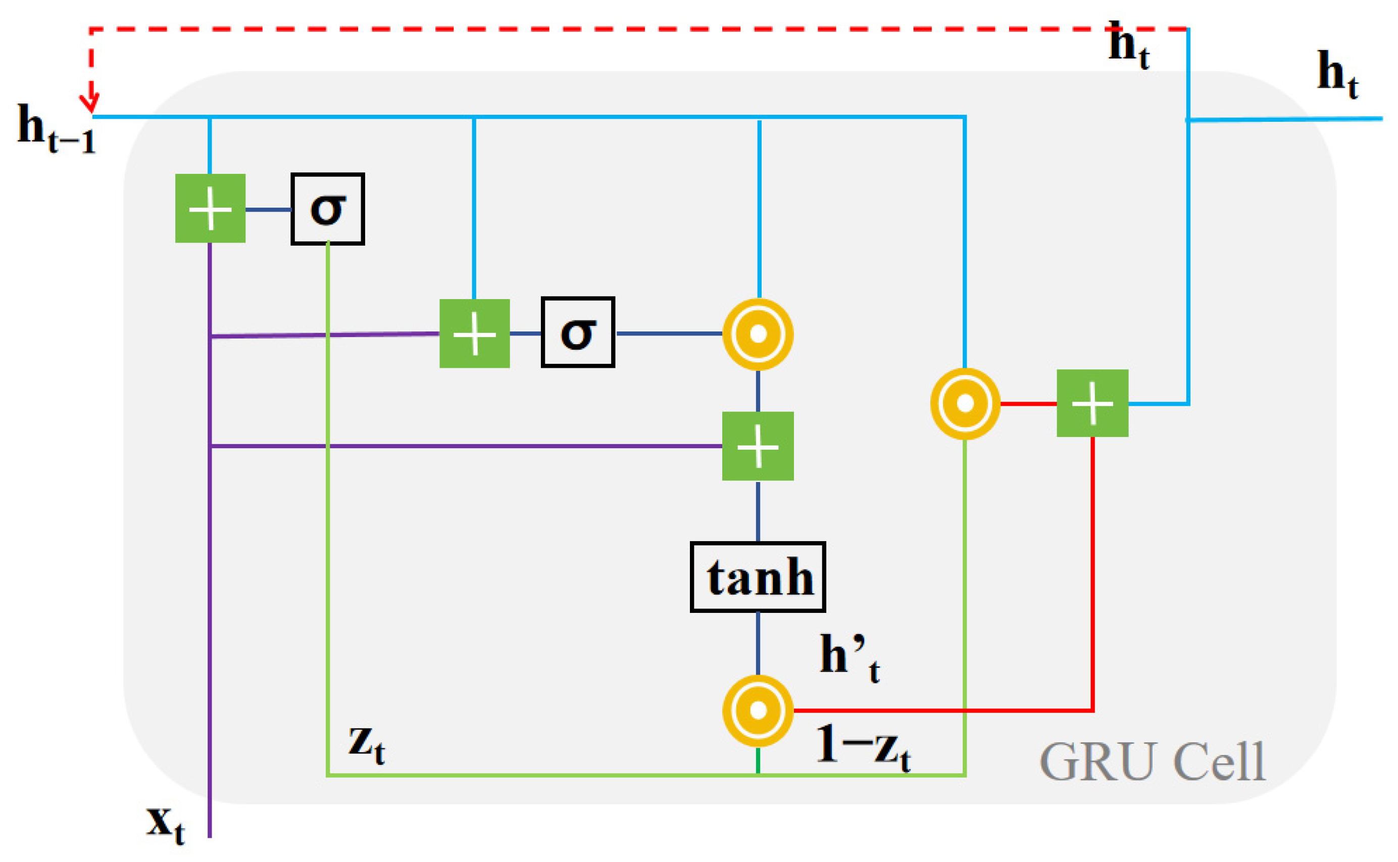
2.2. GRU
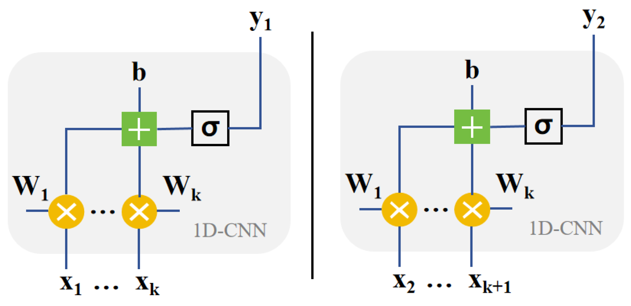
2.3. CNN and Parallelization
3. Experiment Setup and Network Training
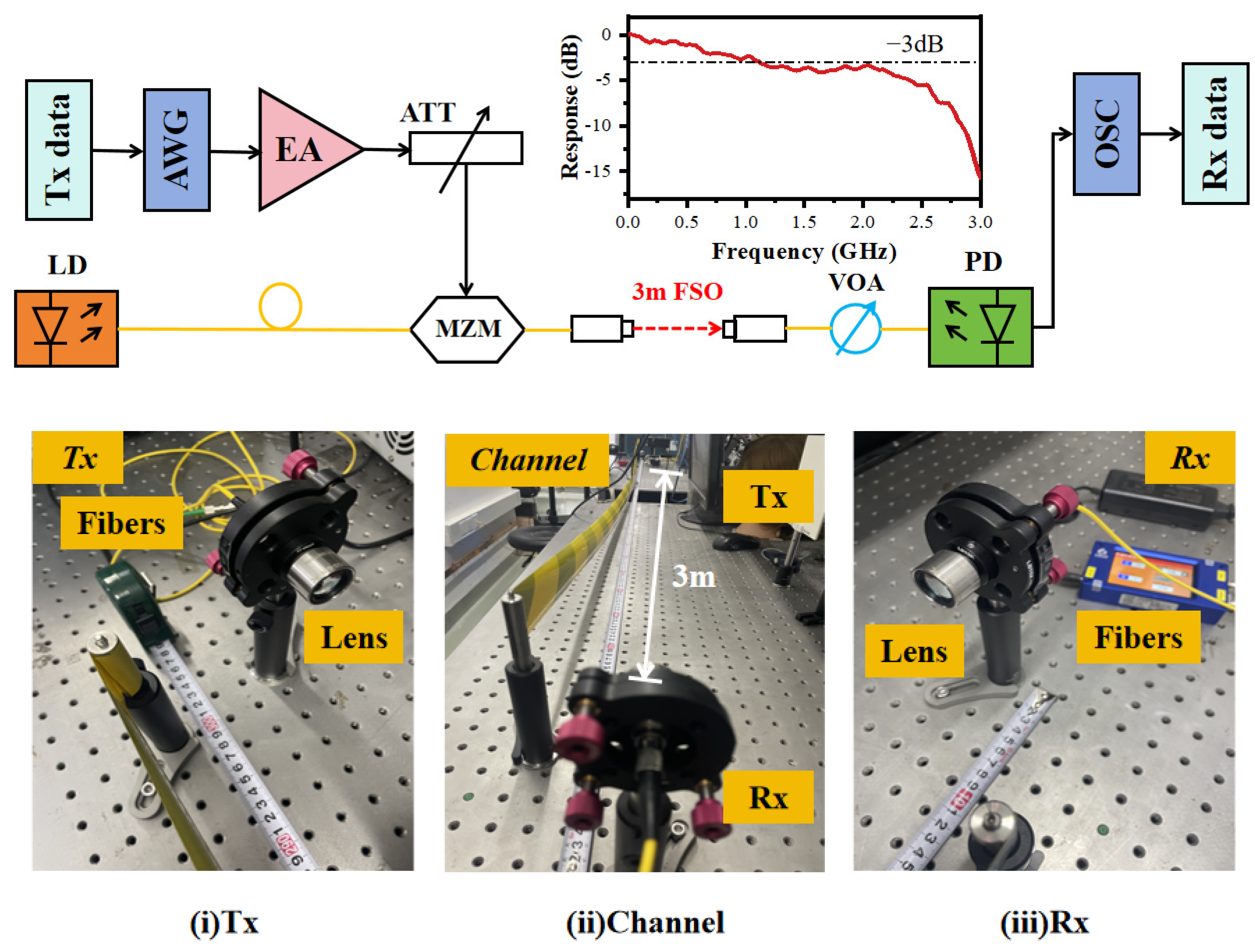
3.1. Experimental System Setup
3.2. Network Training
4. Results and Discussion
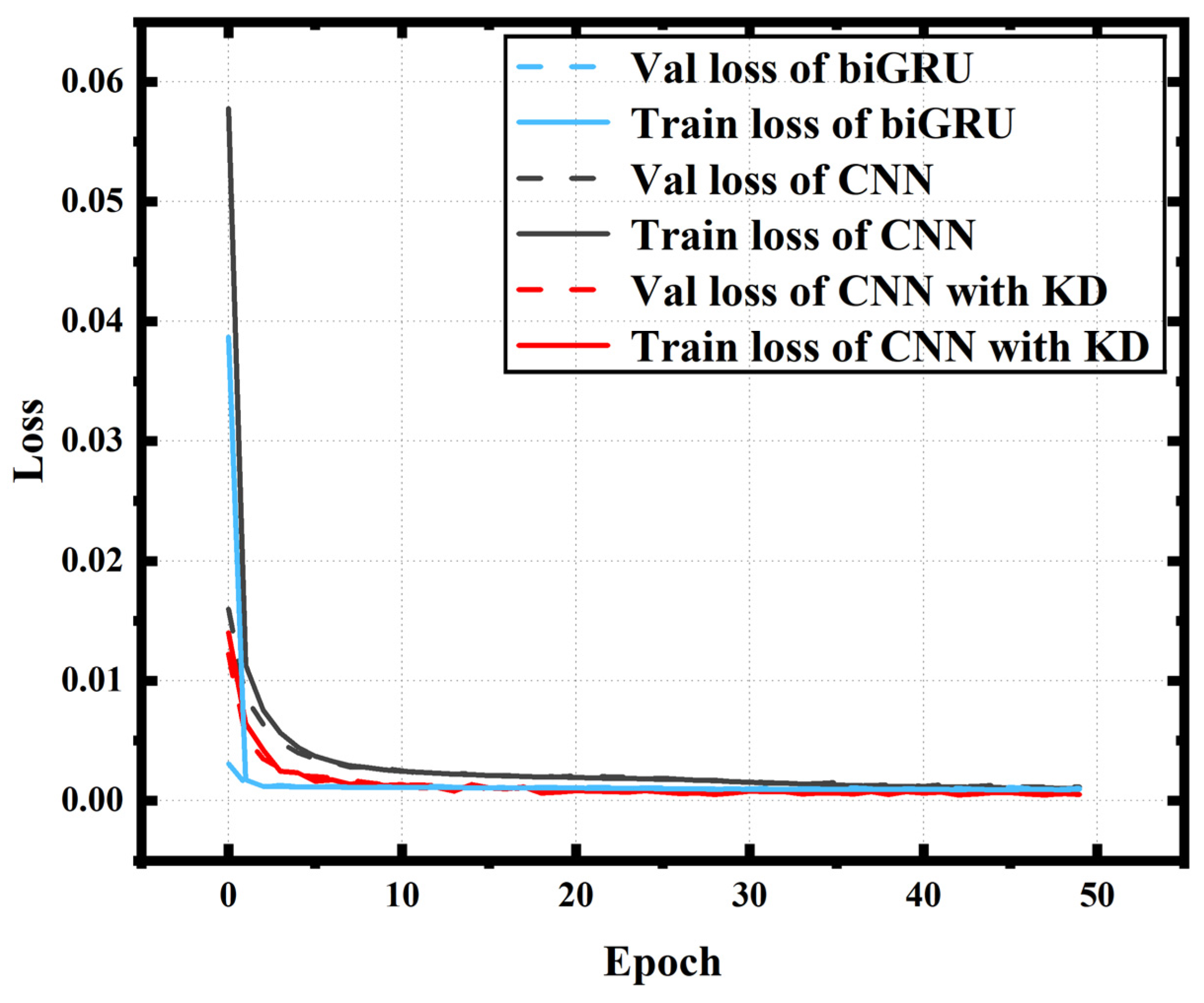
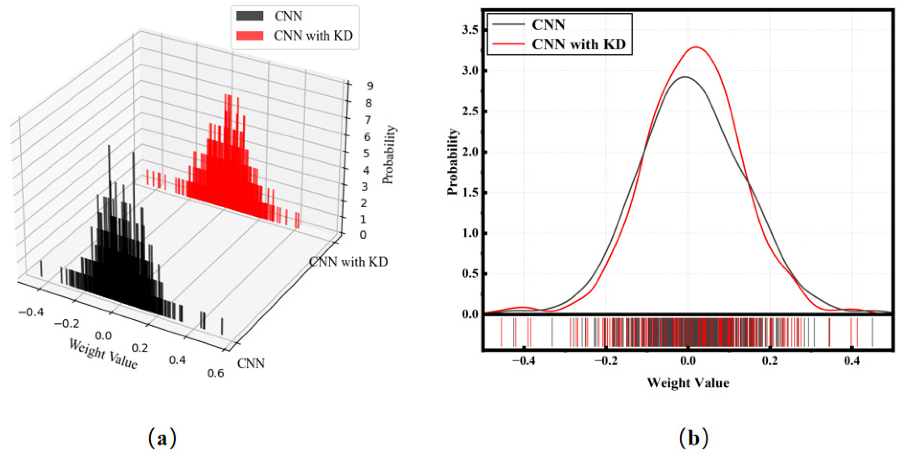
4.1. The Role of Knowledge Distillation
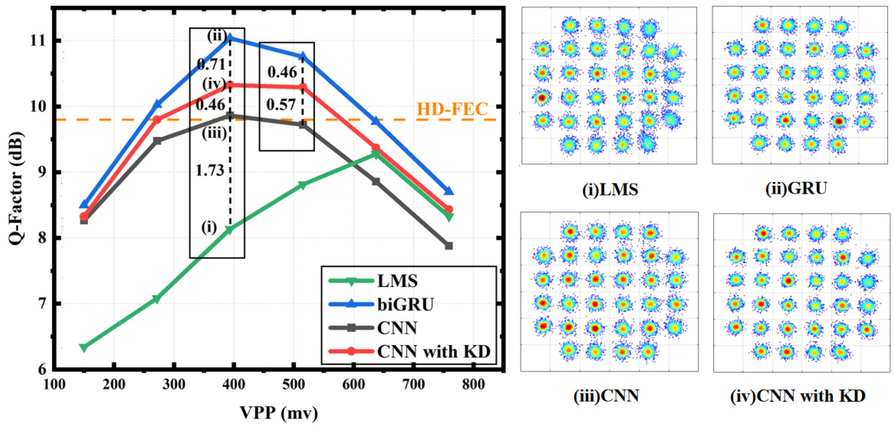
4.2. Equalization Performance
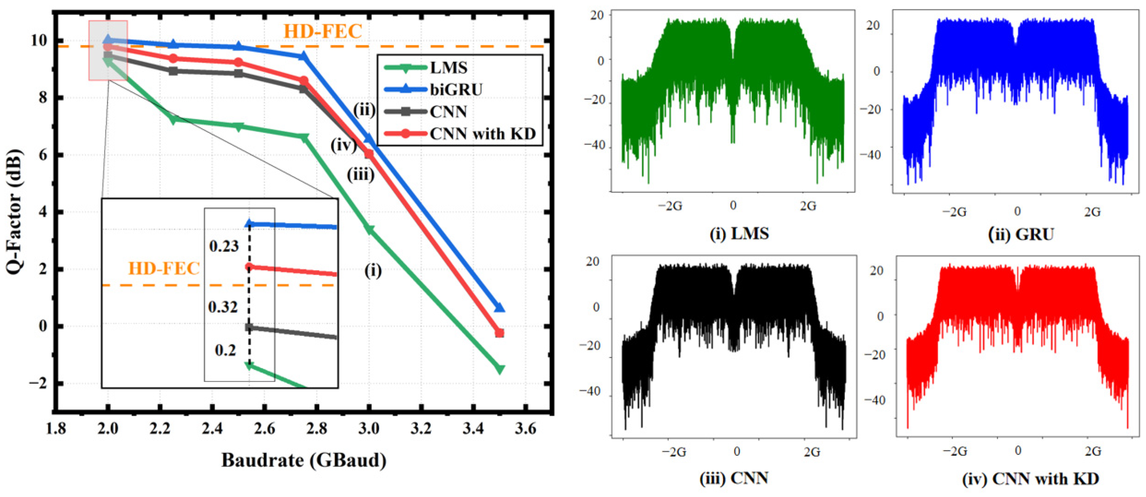
4.3. Speed Performance
5. Conclusions
Author Contributions
Funding
Institutional Review Board Statement
Informed Consent Statement
Data Availability Statement
Conflicts of Interest
References
- Chi, N.; Zhou, Y.; Wei, Y.; Hu, F. Visible light communication in 6G: Advances, challenges, and prospects. IEEE Veh. Technol. Mag. 2020, 15, 93–102. [Google Scholar] [CrossRef]
- Cartledge, J.C.; Guiomar, F.P.; Kschischang, F.R.; Liga, G.; Yankov, M.P. Digital signal processing for fiber nonlinearities. Opt. Express 2017, 25, 1916–1936. [Google Scholar] [CrossRef] [PubMed]
- Ibnkahla, M. Applications of neural networks to digital communications—A survey. Signal Process. 2000, 80, 1185–1215. [Google Scholar] [CrossRef]
- Freire, P.J.; Osadchuk, Y.; Spinnler, B.; Napoli, A.; Schairer, W.; Costa, N.; Prilepsky, J.E.; Turitsyn, S.K. Performance versus complexity study of neural network equalizers in coherent optical systems. J. Light. Technol. 2021, 39, 6085–6096. [Google Scholar] [CrossRef]
- Deligiannidis, S.; Bogris, A.; Mesaritakis, C.; Kopsinis, Y.J. Compensation of fiber nonlinearities in digital coherent systems leveraging long short-term memory neural networks. J. Light. Technol. 2020, 38, 5991–5999. [Google Scholar] [CrossRef]
- Deligiannidis, S.; Mesaritakis, C.; Bogris, A. Performance and complexity analysis of bi-directional recurrent neural network models versus volterra nonlinear equalizers in digital coherent systems. J. Light. Technol. 2021, 39, 5791–5798. [Google Scholar] [CrossRef]
- Lee, S.; Jha, D.; Agrawal, A.; Choudhary, A.; Liao, W.K. Parallel Deep Convolutional Neural Network Training by Exploiting the Overlapping of Computation and Communication. In Proceedings of the IEEE International Conference on High Performance Computing, Jaipur, India, 18–21 December 2017. [Google Scholar]
- Hinton, G.; Vinyals, O.; Dean, J. Distilling the knowledge in a neural network. arXiv 2015, arXiv:1503.02531. [Google Scholar]
- Xu, Q.; Chen, Z.; Ragab, M.; Wang, C.; Wu, M.; Li, X. Contrastive adversarial knowledge distillation for deep model compression in time-series regression tasks. Neurocomputing 2022, 485, 242–251. [Google Scholar] [CrossRef]
- Freire, P.J.; Napoli, A.; Ron, D.A.; Spinnler, B.; Anderson, M.; Schairer, W.; Bex, T.; Costa, N.; Turitsyn, S.K.; Prilepsky, J.E. Reducing computational complexity of neural networks in optical channel equalization: From concepts to implementation. J. Light. Technol. 2023, 41, 4557–4581. [Google Scholar] [CrossRef]
- Takamoto, M.; Morishita, Y.; Imaoka, H. An efficient method of training small models for regression problems with knowledge distillation. In Proceedings of the 2020 IEEE Conference on Multimedia Information Processing and Retrieval (MIPR), Shenzhen, China, 6–8 August 2020; pp. 67–72. [Google Scholar]
- Xiang, J.; Colburn, S.; Majumdar, A.; Shlizerman, E. Knowledge distillation circumvents nonlinearity for optical convolutional neural networks. Appl. Opt. 2022, 61, 2173–2183. [Google Scholar] [CrossRef] [PubMed]
- Ma, H.; Yang, S.; Wu, R.; Hao, X.; Long, H.; He, G. Knowledge distillation-based performance transferring for LSTM-RNN model acceleration. Signal Image Video Process. 2022, 16, 1541–1548. [Google Scholar] [CrossRef]
- Sherstinsky, A. Fundamentals of recurrent neural network (RNN) and long short-term memory (LSTM) network. Phys. D Nonlinear Phenom. 2020, 404, 132306. [Google Scholar] [CrossRef]
- Nosouhian, S.; Nosouhian, F.; Khoshouei, A.K. A review of recurrent neural network architecture for sequence learning: Comparison between LSTM and GRU. Preprints 2021, 2021070252. [Google Scholar] [CrossRef]
- Graves, A.; Schmidhuber, J. Framewise phoneme classification with bidirectional LSTM and other neural network architectures. Neural Netw. 2005, 18, 602–610. [Google Scholar] [CrossRef] [PubMed]
- Hamad, R.A.; Kimura, M.; Yang, L.; Woo, W.L.; Wei, B. Dilated causal convolution with multi-head self attention for sensor human activity recognition. Neural Comput. Appl. 2021, 33, 13705–13722. [Google Scholar] [CrossRef]
- Gong, S.; Wang, Z.; Sun, T.; Zhang, Y.; Smith, C.D.; Xu, L.; Liu, J. Dilated fcn: Listening longer to hear better. In Proceedings of the 2019 IEEE Workshop on Applications of Signal Processing to Audio and Acoustics (WASPAA), New Paltz, NY, USA, 20–23 October 2019; pp. 254–258. [Google Scholar]
- Zhen, X.; Chakraborty, R.; Vogt, N.; Bendlin, B.B.; Singh, V. Dilated convolutional neural networks for sequential manifold-valued data. In Proceedings of the IEEE/CVF International Conference on Computer Vision, Seoul, Republic of Korea, 27 October–2 November 2019; pp. 10621–10631. [Google Scholar]
- Maas, A.L.; Hannun, A.Y.; Ng, A.Y. Rectifier nonlinearities improve neural network acoustic models. In Proceedings of the 30th International Conference on Machine Learning, Atlanta, GA, USA, 16–21 June 2013; p. 3. [Google Scholar]
- Liu, L.; Xiao, S.; Fang, J.; Zhang, L.; Hu, W. High performance and cost effective CO-OFDM system aided by polar code. Opt. Express 2017, 25, 2763–2770. [Google Scholar] [CrossRef] [PubMed]


| Number of Trainable Parameters | Time per Process (s) | |
|---|---|---|
| 1D-CNN with KD | 961 | 0.49 |
| biGRU | 126,281 | 14.36 |
Disclaimer/Publisher’s Note: The statements, opinions and data contained in all publications are solely those of the individual author(s) and contributor(s) and not of MDPI and/or the editor(s). MDPI and/or the editor(s) disclaim responsibility for any injury to people or property resulting from any ideas, methods, instructions or products referred to in the content. |
© 2024 by the authors. Licensee MDPI, Basel, Switzerland. This article is an open access article distributed under the terms and conditions of the Creative Commons Attribution (CC BY) license (https://creativecommons.org/licenses/by/4.0/).
Share and Cite
Zhu, Y.; Wei, Y.; Chen, C.; Chi, N.; Shi, J. Minimalist Deployment of Neural Network Equalizers in a Bandwidth-Limited Optical Wireless Communication System with Knowledge Distillation. Sensors 2024, 24, 1612. https://doi.org/10.3390/s24051612
Zhu Y, Wei Y, Chen C, Chi N, Shi J. Minimalist Deployment of Neural Network Equalizers in a Bandwidth-Limited Optical Wireless Communication System with Knowledge Distillation. Sensors. 2024; 24(5):1612. https://doi.org/10.3390/s24051612
Chicago/Turabian StyleZhu, Yiming, Yuan Wei, Chaoxu Chen, Nan Chi, and Jianyang Shi. 2024. "Minimalist Deployment of Neural Network Equalizers in a Bandwidth-Limited Optical Wireless Communication System with Knowledge Distillation" Sensors 24, no. 5: 1612. https://doi.org/10.3390/s24051612