
A Robust Approach Assisted by Signal Quality Assessment for Fetal Heart Rate Estimation from Doppler Ultrasound Signal
 , ,
, ,
Abstract
:1. Introduction
- We combine time and frequency information using STFT for DUS signal pre-processing so that the ACF-based FHR estimation algorithm does not focus only on a single domain as in previous works.
- This method is robust to DUS recordings of different qualities because it is supported by DUS SQA.
- An unsupervised representation learning-based DUS SQA approach is proposed in this paper, which eliminates the need for a large dataset of quality labels. Furthermore, representation learning enables our method to exploit deeper information than human-defined features.
2. Related Work
- The ACF calculations in these existing works only focus on one domain, time, or frequency. Thus, the information about the other domain may be lost during the calculation.
- Large labeled datasets are usually required for these research works based on supervised machine learning methods. However, there are few DUS datasets with quality annotations. In addition, annotation of DUS quality levels is laborious and requires expert knowledge.
- The human-defined signal quality features used in these works limit the ability to mine deeper signal quality information in DUS signals.
- These existing methods simply eliminate the estimated FHRs from the detected low-quality DUS signal segments, which may result in a reduction in the proportion of reserved FHRs to all estimated FHRs in each recording.
3. Preliminaries
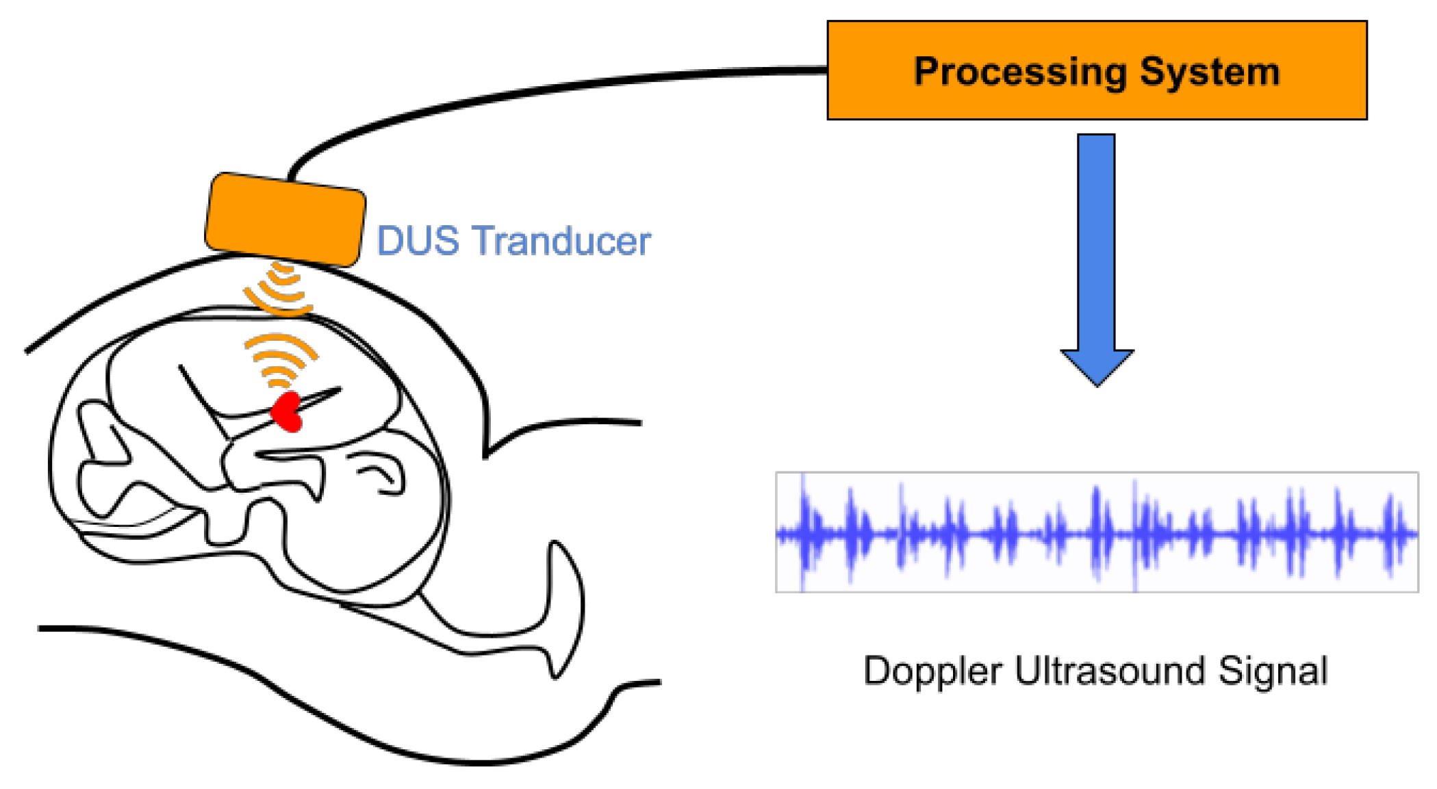
3.1. Doppler Ultrasound (DUS) Signal
3.2. Autocorrelation Function (ACF)
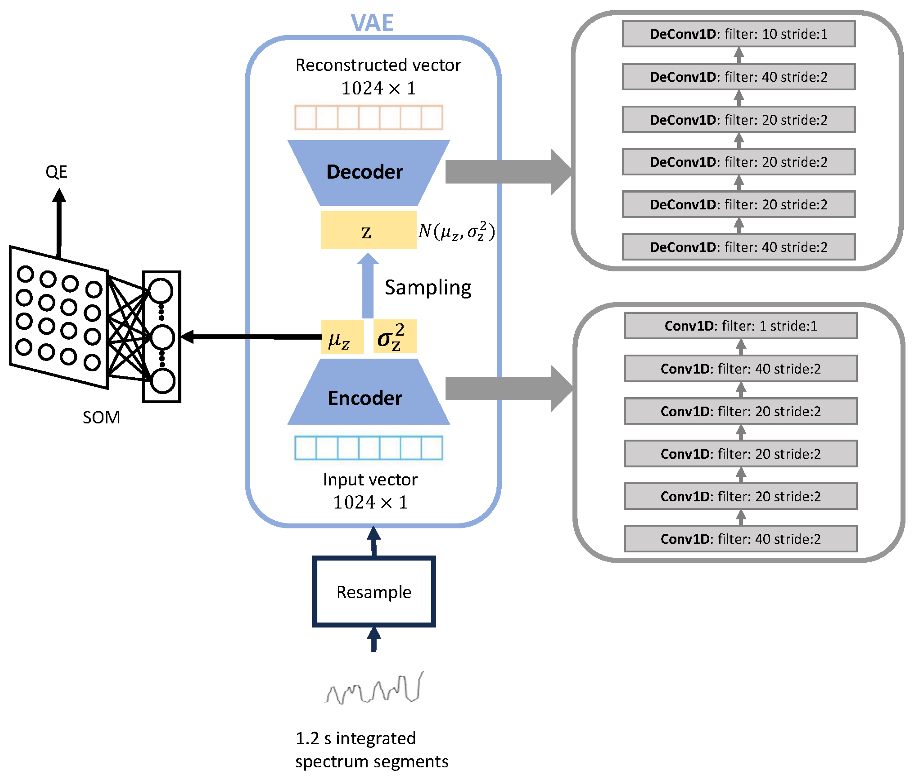
3.3. Variational Autoencoder (VAE)
3.4. Self-Organizing Map (SOM)
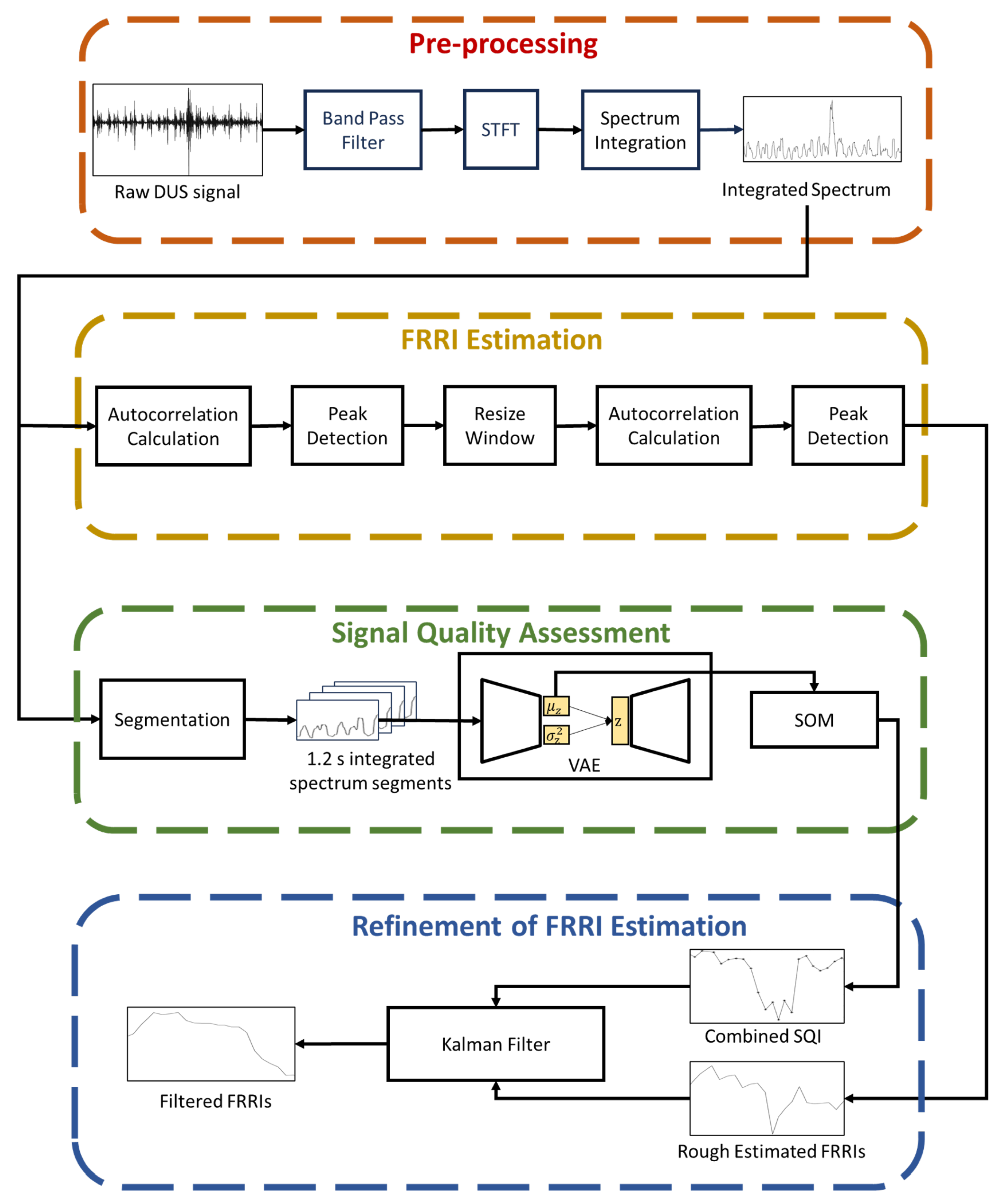
4. Proposed Method
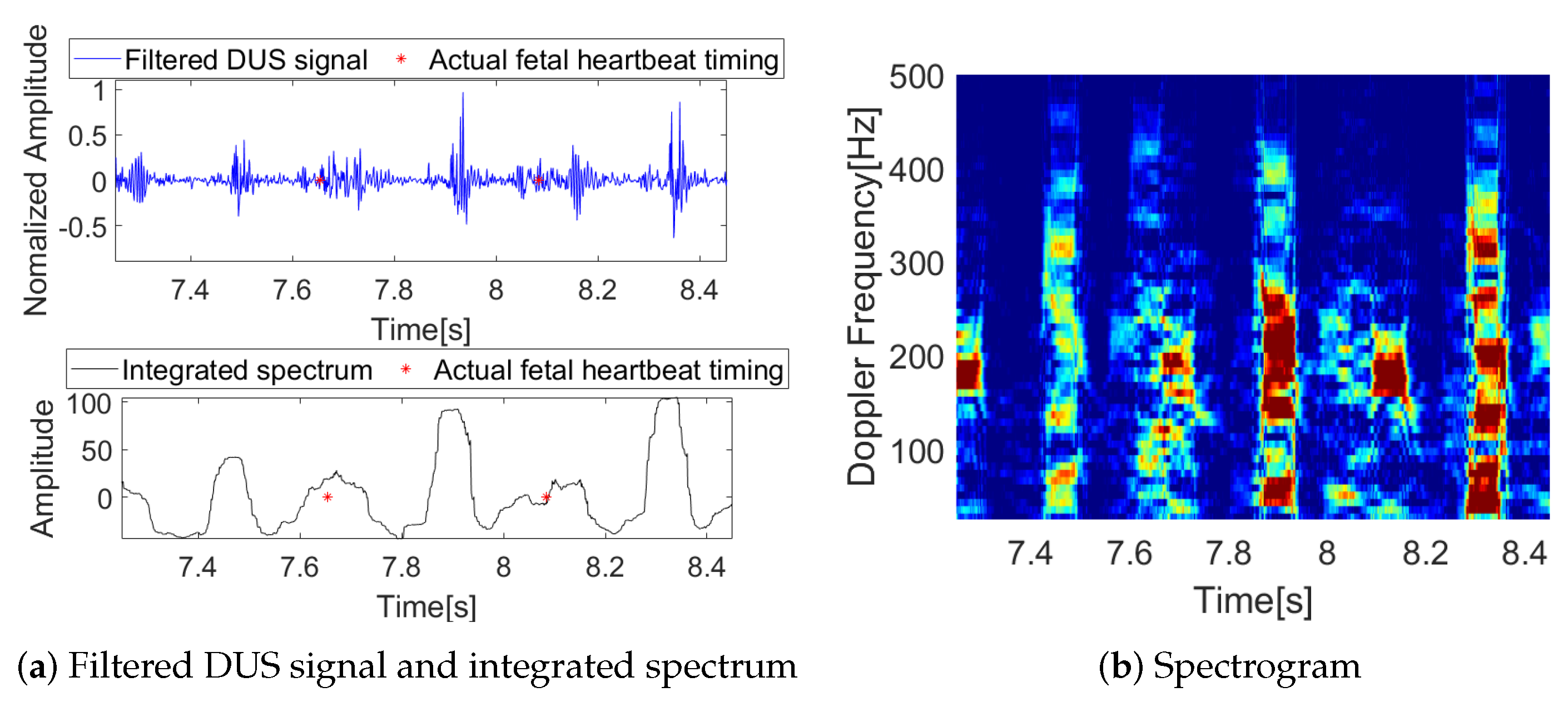
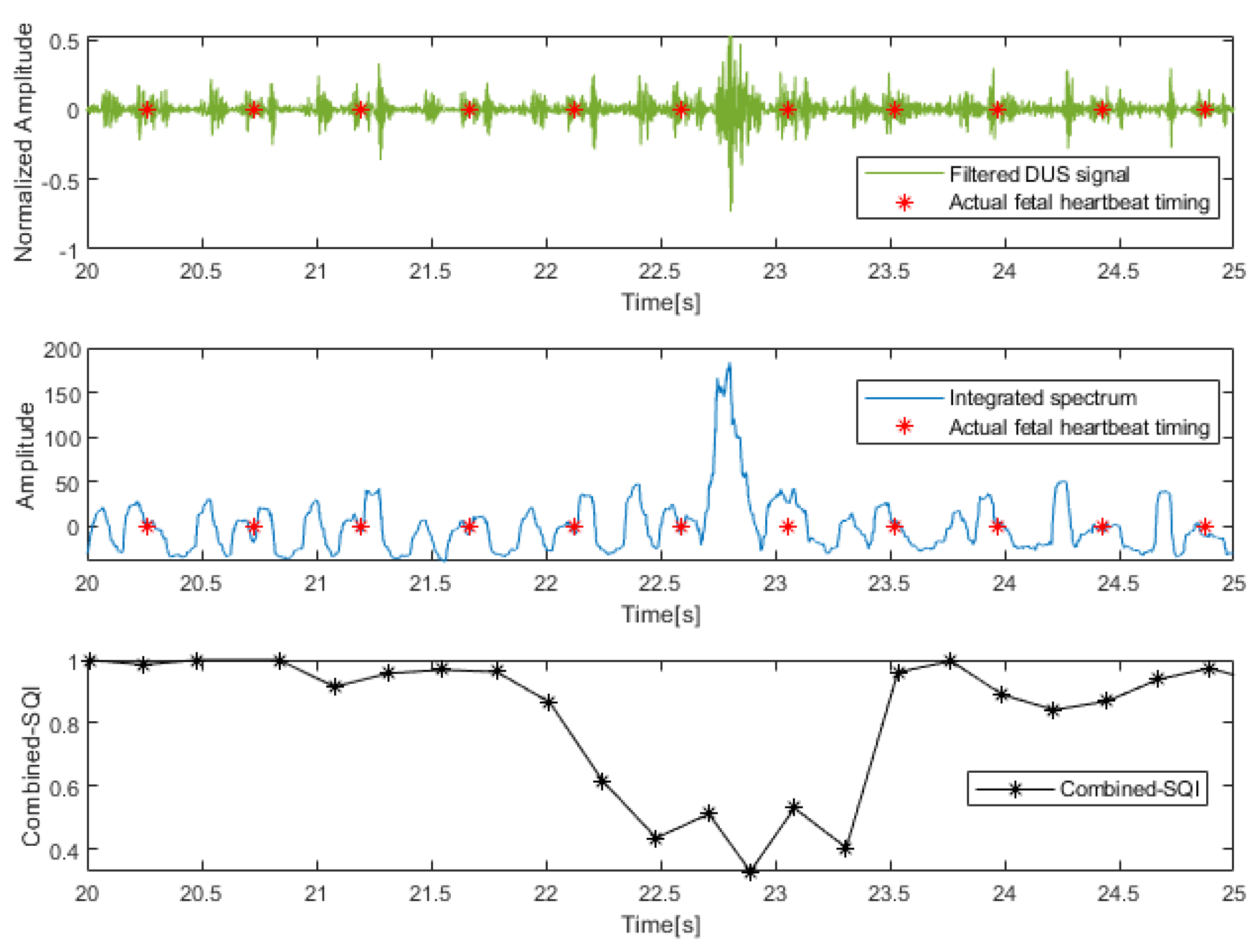
4.1. Pre-Processing
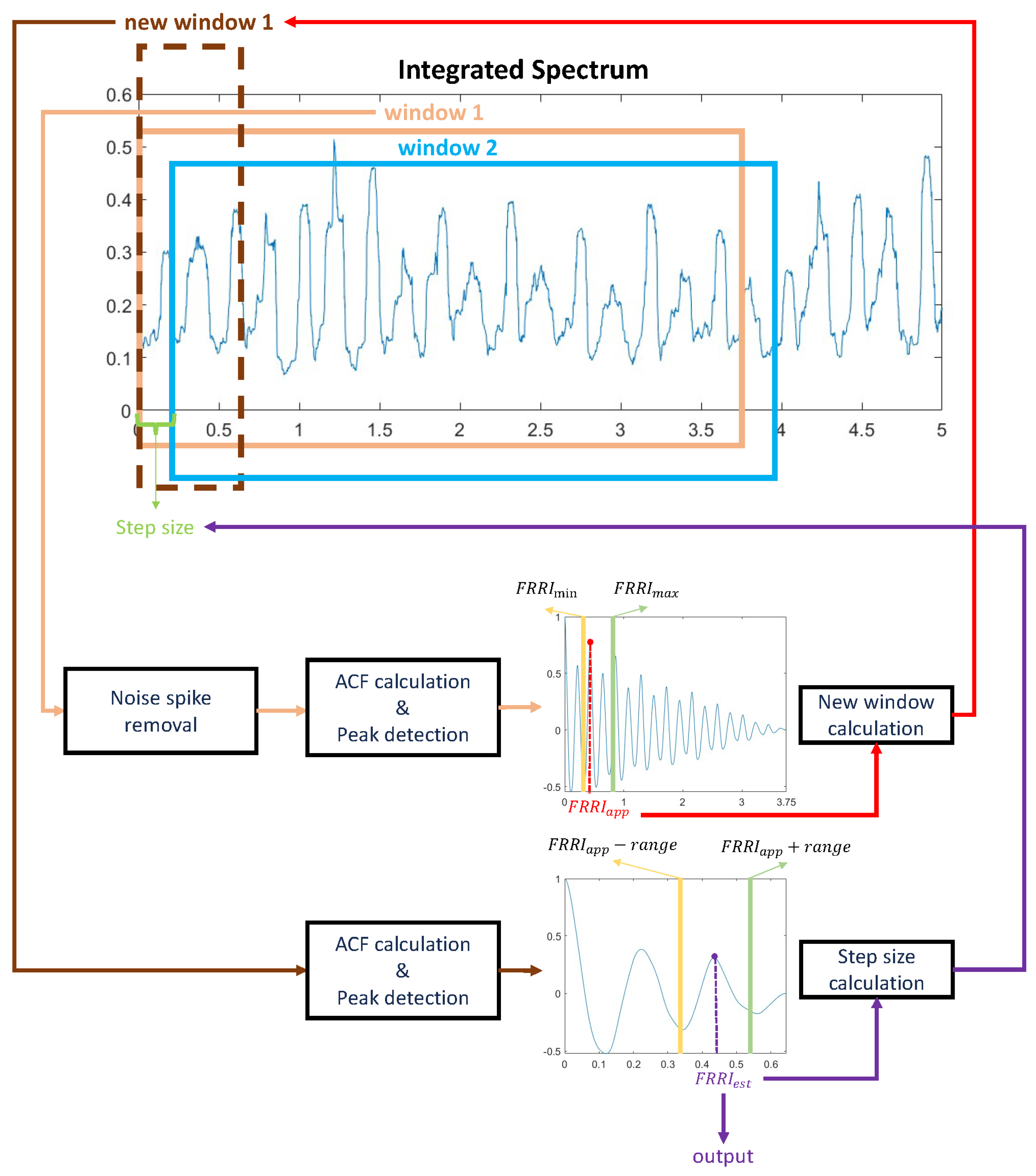
4.2. FRRI Estimation
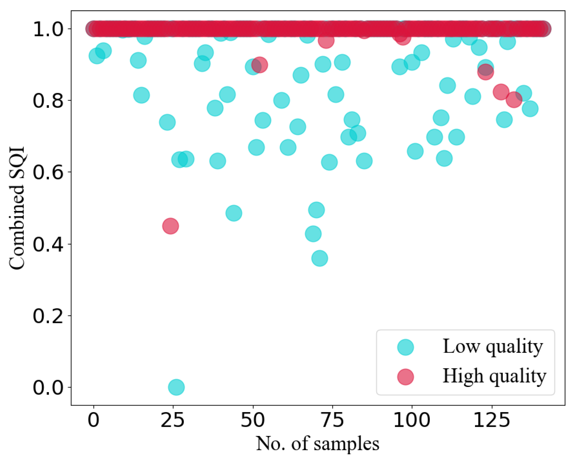
4.3. SQA
4.4. FRRI Estimation Refinement
5. Results and Discussion
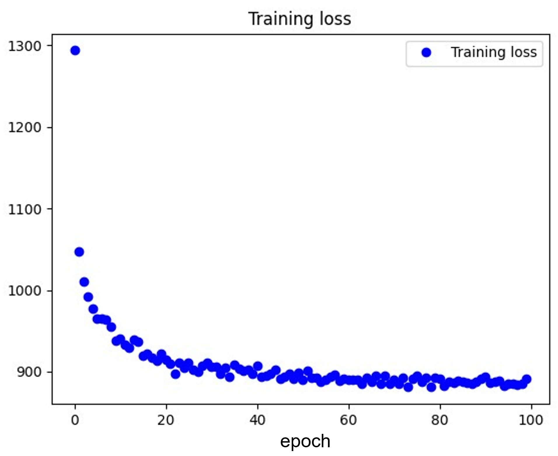
5.1. Experimental Setup
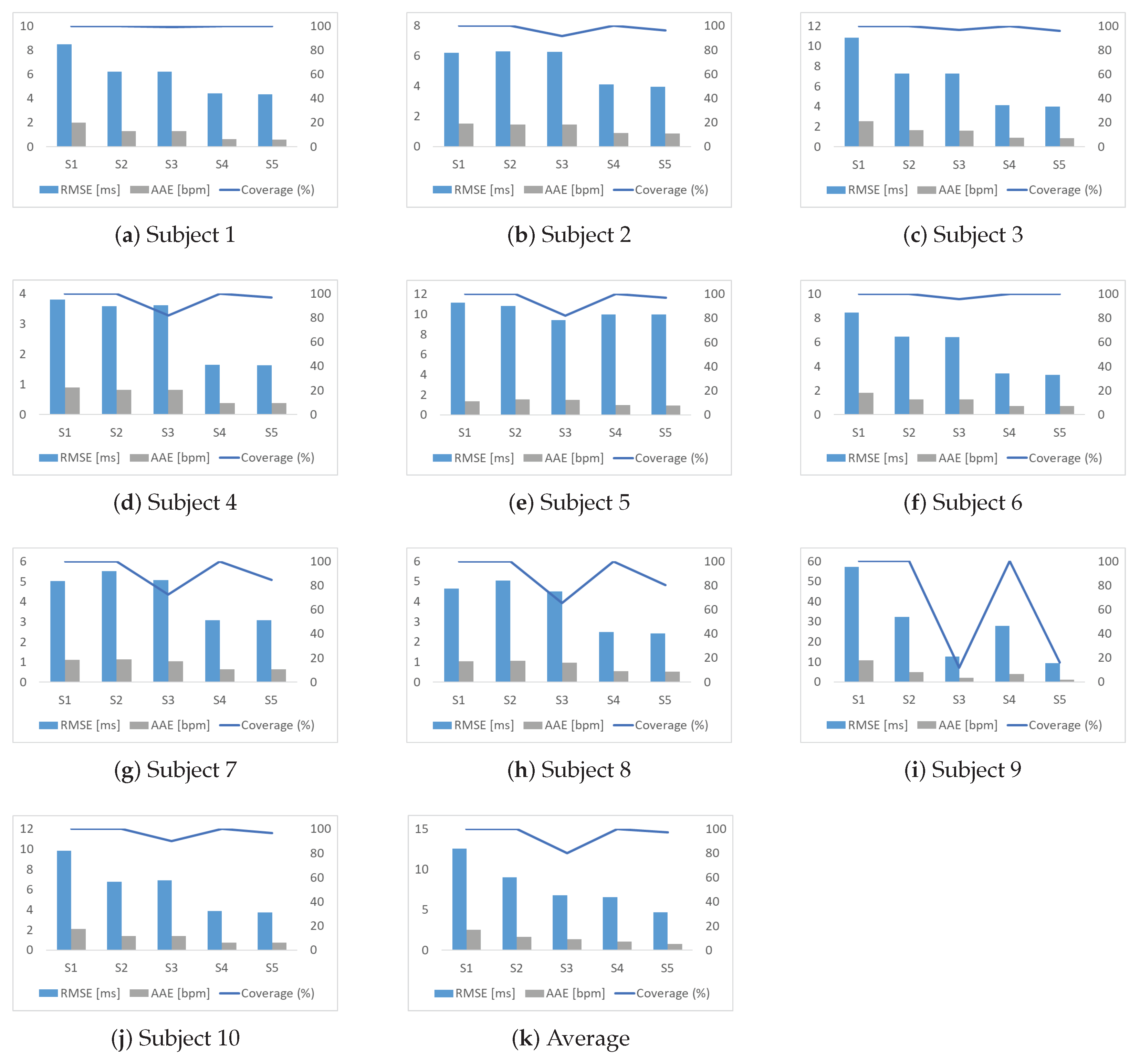
- Root mean square error (RMSE): RMSE is calculated between the estimated value and the ground truth value of FRRI, which is calculated as follows:
- Averaged absolute error (AAE): AAE is calculated between the estimated value and the ground truth value of FHR, which is calculated as follows:
- Coverage: Since some rough FRRI estimates may be removed based on the results of the SQA, the ratio of reserved FRRI estimates to all FRRI estimates is a critical indicator of whether as many FRRI estimates as possible have been retained.
- Use the method proposed by Valderrama et al. [7].
- FHR estimation only: We performed only two steps to obtain rough FRRI estimates, including preprocessing and FRRI estimation (described in Section 4.1 and Section 4.2).
- Remove unreliable FRRIs: We eliminate the unreliable rough FRRIs if the corresponding combined SQI is less than the 8th decile of all combined SQI values.
- Use conventional KF: A conventional KF with a fixed noise covariance metric was applied to the rough FRRI estimates.
- Proposed method: The four steps described in Section 4 are all used to estimate and refine FRRIs.
5.2. Experimental Results
5.3. Limitation and Future Works
6. Conclusions
Author Contributions
Funding
Institutional Review Board Statement
Informed Consent Statement
Data Availability Statement
Conflicts of Interest
References
- Grivell, R.M.; Alfirevic, Z.; Gyte, G.M.; Devane, D. Antenatal cardiotocography for fetal assessment. Cochrane Database Syst. Rev. 2015, 9, CD007863. [Google Scholar] [CrossRef] [PubMed]
- Bakker, P.; Colenbrander, G.; Verstraeten, A.; Van Geijn, H. The quality of intrapartum fetal heart rate monitoring. Eur. J. Obstet. Gynecol. Reprod. Biol. 2004, 116, 22–27. [Google Scholar] [CrossRef] [PubMed]
- Sameni, R.; Clifford, G.D. A review of fetal ECG signal processing; issues and promising directions. Open Pacing Electrophysiol. Ther. J. 2010, 3, 4. [Google Scholar] [CrossRef] [PubMed]
- Hamelmann, P.; Vullings, R.; Kolen, A.F.; Bergmans, J.W.; van Laar, J.O.; Tortoli, P.; Mischi, M. Doppler ultrasound technology for fetal heart rate monitoring: A review. IEEE Trans. Ultrason. Ferroelectr. Freq. Control. 2019, 67, 226–238. [Google Scholar] [CrossRef] [PubMed]
- Peters, C.H.; ten Broeke, E.D.; Andriessen, P.; Vermeulen, B.; Berendsen, R.C.; Wijn, P.F.; Oei, S.G. Beat-to-beat detection of fetal heart rate: Doppler ultrasound cardiotocography compared to direct ECG cardiotocography in time and frequency domain. Physiol. Meas. 2004, 25, 585. [Google Scholar] [CrossRef] [PubMed]
- Jezewski, J.; Roj, D.; Wrobel, J.; Horoba, K. A novel technique for fetal heart rate estimation from Doppler ultrasound signal. Biomed. Eng. Online 2011, 10, 1–17. [Google Scholar] [CrossRef] [PubMed]
- Valderrama, C.E.; Stroux, L.; Katebi, N.; Paljug, E.; Hall-Clifford, R.; Rohloff, P.; Marzbanrad, F.; Clifford, G.D. An open source autocorrelation-based method for fetal heart rate estimation from one-dimensional Doppler ultrasound. Physiol. Meas. 2019, 40, 025005. [Google Scholar] [CrossRef] [PubMed]
- Rouvre, D.; Kouamé, D.; Tranquart, F.; Pourcelot, L. Empirical mode decomposition (EMD) for multi-gate, multi-transducer ultrasound Doppler fetal heart monitoring. In Proceedings of the the 5th IEEE International Symposium on Signal Processing and Information Technology, Athens, Greece, 21 December 2005; pp. 208–212. [Google Scholar]
- Al-Angari, H.M.; Kimura, Y.; Hadjileontiadis, L.J.; Khandoker, A.H. A hybrid EMD-kurtosis method for estimating fetal heart rate from continuous Doppler signals. Front. Physiol. 2017, 8, 641. [Google Scholar] [CrossRef] [PubMed]
- Valderrama, C.E.; Marzbanrad, F.; Stroux, L.; Clifford, G.D. Template-based quality assessment of the Doppler ultrasound signal for fetal monitoring. Front. Physiol. 2017, 8, 511. [Google Scholar] [CrossRef]
- Marzbanrad, F.; Kimura, Y.; Endo, M.; Palaniswami, M.; Khandoker, A.H. Classification of Doppler ultrasound signal quality for the application of fetal valve motion identification. In Proceedings of the 2015 Computing in Cardiology Conference (CinC), Nice, France, 6–9 September 2015; pp. 365–368. [Google Scholar]
- Seeuws, N.; De Vos, M.; Bertrand, A. Electrocardiogram quality assessment using unsupervised deep learning. IEEE Trans. Biomed. Eng. 2021, 69, 882–893. [Google Scholar] [CrossRef] [PubMed]
- Pereira, J.; Silveira, M. Learning representations from healthcare time series data for unsupervised anomaly detection. In Proceedings of the 2019 IEEE International Conference on Big Data and Smart Computing (BigComp), Kyoto, Japan, 27 February–2 March 2019; pp. 1–7. [Google Scholar]
- Kohonen, T.; Nieminen, I.T.; Honkela, T. On the quantization error in SOM vs. VQ: A critical and systematic study. In Proceedings of the Advances in Self-Organizing Maps, St. Augustine, FL, USA, 8–10 June 2009; pp. 133–144. [Google Scholar]
- Li, Q.; Mark, R.G.; Clifford, G.D. Robust heart rate estimation from multiple asynchronous noisy sources using signal quality indices and a Kalman filter. Physiol. Meas. 2007, 29, 15. [Google Scholar] [CrossRef] [PubMed]
- Andreotti, F.; Graesser, F.; Malberg, H.; Zaunseder, S. Non-invasive fetal ECG signal quality assessment for multichannel heart rate estimation. IEEE Trans. Biomed. Eng. 2017, 64, 2793–2802. [Google Scholar] [CrossRef] [PubMed]
- Shi, X.; Yamamoto, K.; Ohtsuki, T.; Matsui, Y.; Owada, K. Unsupervised Representation Learning-based Doppler Ultrasound Signal Quality Assessment. In Proceedings of the 2022 IEEE Global Communications Conference, Rio de Janeiro, Brazil, 4–8 December 2022; pp. 2254–2259. [Google Scholar]
- Roy, M.S.; Gupta, R.; Sharma, K.D. Photoplethysmogram signal quality evaluation by unsupervised learning approach. In Proceedings of the 2020 IEEE Applied Signal Processing Conference (ASPCON), Kolkata, India, 7–9 October 2020; pp. 6–10. [Google Scholar]
- Lei, Q.; Yi, J.; Vaculin, R.; Wu, L.; Dhillon, I.S. Similarity preserving representation learning for time series clustering. arXiv 2017, arXiv:1702.03584. [Google Scholar]
- Heckert, N.A.; Filliben, J.J. Nist/Sematech e-Handbook of Statistical Methods; Chapter 1: Exploratory Data Analysis; NIST: Gaithersburg, MD, USA, 2003. [Google Scholar]
- Rui, T.; Zhang, S.; Ren, T.; Tang, J.; Zou, J. Data Reconstruction based on supervised deep auto-encoder. In Proceedings of the Pacific Rim Conference on Multimedia, Hefei, China, 21–22 September 2018; pp. 869–879. [Google Scholar]
- Kingma, D.P.; Welling, M. Auto-encoding variational bayes. arXiv 2013, arXiv:1312.6114. [Google Scholar]
- Ghosal, P.; Sarkar, D.; Kundu, S.; Roy, S.; Sinha, A.; Ganguli, S. Ecg beat quality assessment using self organizing map. In Proceedings of the 2017 4th International Conference on Opto-Electronics and Applied Optics (Optronix), Kolkata, India, 2–3 November 2017; pp. 1–5. [Google Scholar]
- Yamamoto, K.; Toyoda, K.; Ohtsuki, T. Spectrogram-based non-contact RRI estimation by accurate peak detection algorithm. IEEE Access 2018, 6, 60369–60379. [Google Scholar] [CrossRef]
- Schmidt, S.; Toft, E.; Holst-Hansen, C.; Graff, C.; Struijk, J. Segmentation of heart sound recordings from an electronic stethoscope by a duration dependent Hidden-Markov Model. In Proceedings of the 2008 Computers in Cardiology, Bologna, Italy, 14–17 September 2008; pp. 345–348. [Google Scholar] [CrossRef]
- Chiang, H.T.; Hsieh, Y.Y.; Fu, S.W.; Hung, K.H.; Tsao, Y.; Chien, S.Y. Noise reduction in ECG signals using fully convolutional denoising autoencoders. IEEE Access 2019, 7, 60806–60813. [Google Scholar] [CrossRef]
- Kalman, R.E. A New Approach to Linear Filtering and Prediction Problems. J. Basic Eng. 1960, 82, 35–45. [Google Scholar] [CrossRef]
- Liu, S.H.; Li, R.X.; Wang, J.J.; Chen, W.; Su, C.H. Classification of photoplethysmographic signal quality with deep convolution neural networks for accurate measurement of cardiac stroke volume. Appl. Sci. 2020, 10, 4612. [Google Scholar] [CrossRef]


| 1 | 2 | 3 | 4 | 5 | 6 | 7 | 8 | 9 | 10 | Average | ||
|---|---|---|---|---|---|---|---|---|---|---|---|---|
| Valderrama et al. [7] | RMSE [ms] | 8.46 | 6.21 | 10.81 | 3.80 | 11.12 | 8.46 | 5.02 | 4.64 | 57.10 | 9.83 | 12.54 |
| AAE [bpm] | 1.98 | 1.51 | 2.54 | 0.90 | 1.34 | 1.80 | 1.11 | 1.04 | 10.79 | 2.09 | 2.51 | |
| Coverage (%) | 100.00 | 100.00 | 100.00 | 100.00 | 100.00 | 100.00 | 100.00 | 100.00 | 100.00 | 100.00 | 100.00 | |
| FHR estimation only | RMSE [ms] | 6.20 | 6.30 | 7.26 | 3.58 | 10.83 | 6.48 | 5.52 | 5.03 | 32.36 | 6.78 | 9.03 |
| AAE [bpm] | 1.27 | 1.47 | 1.63 | 0.82 | 1.55 | 1.27 | 1.14 | 1.06 | 4.89 | 1.39 | 1.65 | |
| Coverage (%) | 100.00 | 100.00 | 100.00 | 100.00 | 100.00 | 100.00 | 100.00 | 100.00 | 100.00 | 100.00 | 100.00 | |
| Remove unreliable FRRIs | RMSE [ms] | 6.22 | 6.27 | 7.25 | 3.62 | 9.42 | 6.43 | 5.06 | 4.50 | 12.62 | 6.90 | 6.83 |
| AAE [bpm] | 1.27 | 1.45 | 1.61 | 0.82 | 1.48 | 1.26 | 1.04 | 0.97 | 2.06 | 1.40 | 1.34 | |
| Coverage (%) | 99.23 | 91.41 | 96.87 | 81.93 | 95.18 | 95.53 | 72.54 | 65.52 | 11.95 | 89.75 | 79.99 | |
| Use conventional KF | RMSE [ms] | 4.42 | 4.12 | 5.15 | 1.64 | 9.96 | 3.40 | 3.07 | 2.49 | 27.77 | 3.87 | 6.59 |
| AAE [bpm] | 0.63 | 0.90 | 1.01 | 0.37 | 0.96 | 0.73 | 0.64 | 0.54 | 3.83 | 0.74 | 1.03 | |
| Coverage (%) | 100.00 | 100.00 | 100.00 | 100.00 | 100.00 | 100.00 | 100.00 | 100.00 | 100.00 | 100.00 | 100.00 | |
| Proposed method | RMSE [ms] | 4.35 | 3.97 | 5.00 | 1.62 | 9.95 | 3.31 | 3.07 | 2.41 | 9.22 | 3.75 | 4.67 |
| AAE [bpm] | 0.59 | 0.86 | 0.98 | 0.37 | 0.94 | 0.72 | 0.63 | 0.52 | 1.07 | 0.72 | 0.74 | |
| Coverage (%) | 100.00 | 96.06 | 100.00 | 96.77 | 100.00 | 100.00 | 84.71 | 80.35 | 16.00 | 96.69 | 87.06 |
Disclaimer/Publisher’s Note: The statements, opinions and data contained in all publications are solely those of the individual author(s) and contributor(s) and not of MDPI and/or the editor(s). MDPI and/or the editor(s) disclaim responsibility for any injury to people or property resulting from any ideas, methods, instructions or products referred to in the content. |
© 2023 by the authors. Licensee MDPI, Basel, Switzerland. This article is an open access article distributed under the terms and conditions of the Creative Commons Attribution (CC BY) license (https://creativecommons.org/licenses/by/4.0/).
Share and Cite
Shi, X.; Niida, N.; Yamamoto, K.; Ohtsuki, T.; Matsui, Y.; Owada, K. A Robust Approach Assisted by Signal Quality Assessment for Fetal Heart Rate Estimation from Doppler Ultrasound Signal. Sensors 2023, 23, 9698. https://doi.org/10.3390/s23249698
Shi X, Niida N, Yamamoto K, Ohtsuki T, Matsui Y, Owada K. A Robust Approach Assisted by Signal Quality Assessment for Fetal Heart Rate Estimation from Doppler Ultrasound Signal. Sensors. 2023; 23(24):9698. https://doi.org/10.3390/s23249698
Chicago/Turabian StyleShi, Xintong, Natsuho Niida, Kohei Yamamoto, Tomoaki Ohtsuki, Yutaka Matsui, and Kazunari Owada. 2023. "A Robust Approach Assisted by Signal Quality Assessment for Fetal Heart Rate Estimation from Doppler Ultrasound Signal" Sensors 23, no. 24: 9698. https://doi.org/10.3390/s23249698