
Fast Trajectory Tracking Control Algorithm for Autonomous Vehicles Based on the Alternating Direction Multiplier Method (ADMM) to the Receding Optimization of Model Predictive Control (MPC)

Abstract
:1. Introduction
2. MPC-Based Trajectory Tracking Control
2.1. Vehicle Dynamics Model
2.2. Trajectory Tracking Based on Model Predictive Control
3. Implementation of ADMM Algorithm for Trajectory Tracking MPC Problem
3.1. Alternating Direction Method of Multipliers
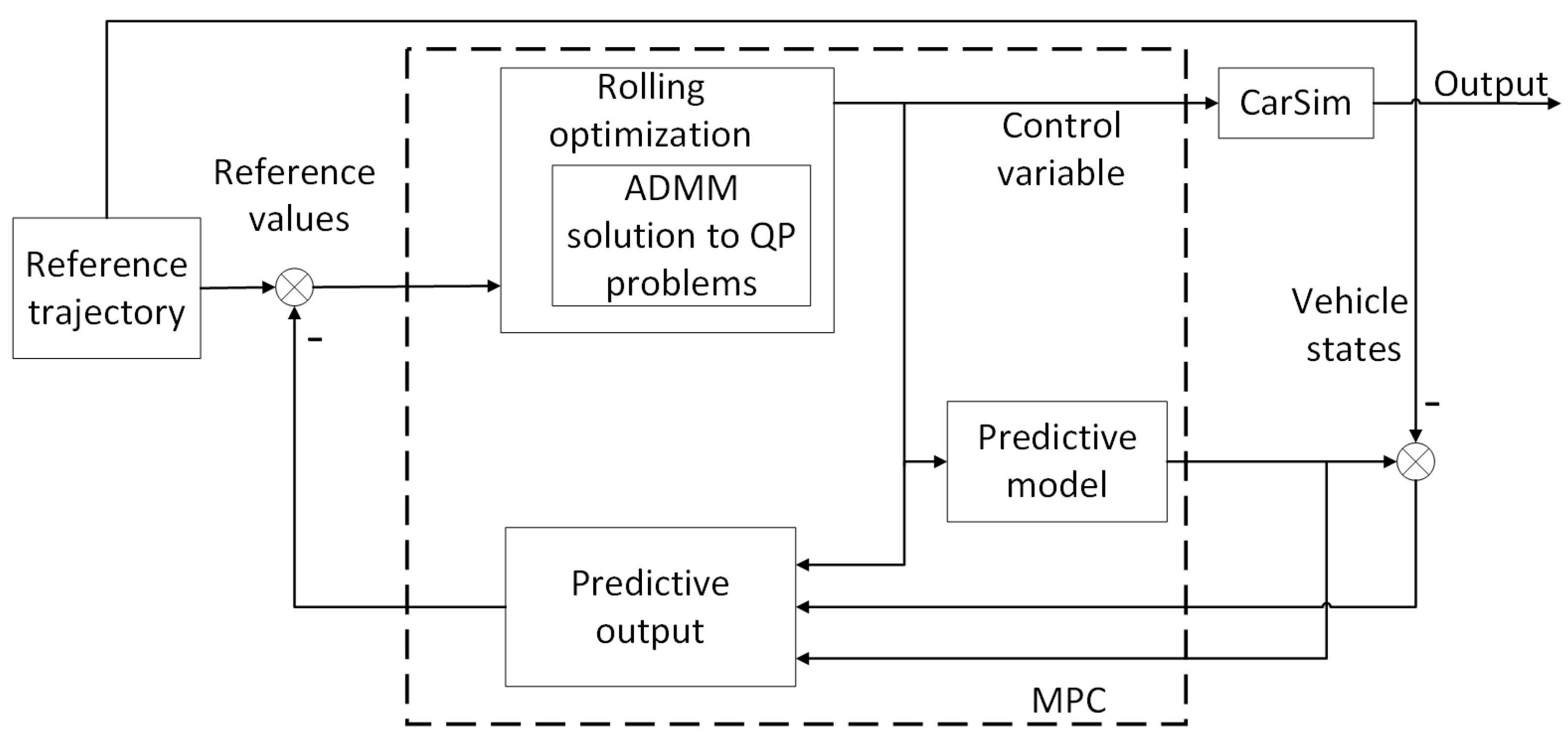
3.2. Model Predictive Controller Based on ADMM Improvement
- (1)
- Initialize the MPC parameter to obtain the system status information at the dth moment.
- (2)
- According to the equation of the state variables of the system and the input and output variables, the objective function is converted into a quadratic programming problem in the form of Equation (14).
- (3)
- Rewrite Equation (14) to form as Equation (22) conforms to the ADMM solution.
- (4)
- The optimal solution obtained at time is used as the initial value of the solution to the time problem.
- (5)
- The variables are updated according to the iterative process of the ADMM algorithm, as shown in Equation (26).
- (6)
- According to Equations (27)–(30), to determine whether the iteration process meets the termination conditions, if it is met, stop the iteration, send the first term in the calculated optimal solution sequence to the control system as input, and enter step (7); if not, continue to iterate until the maximum number of iterations is reached.
- (7)
- Go to the next sampling moment , and repeat step (1).
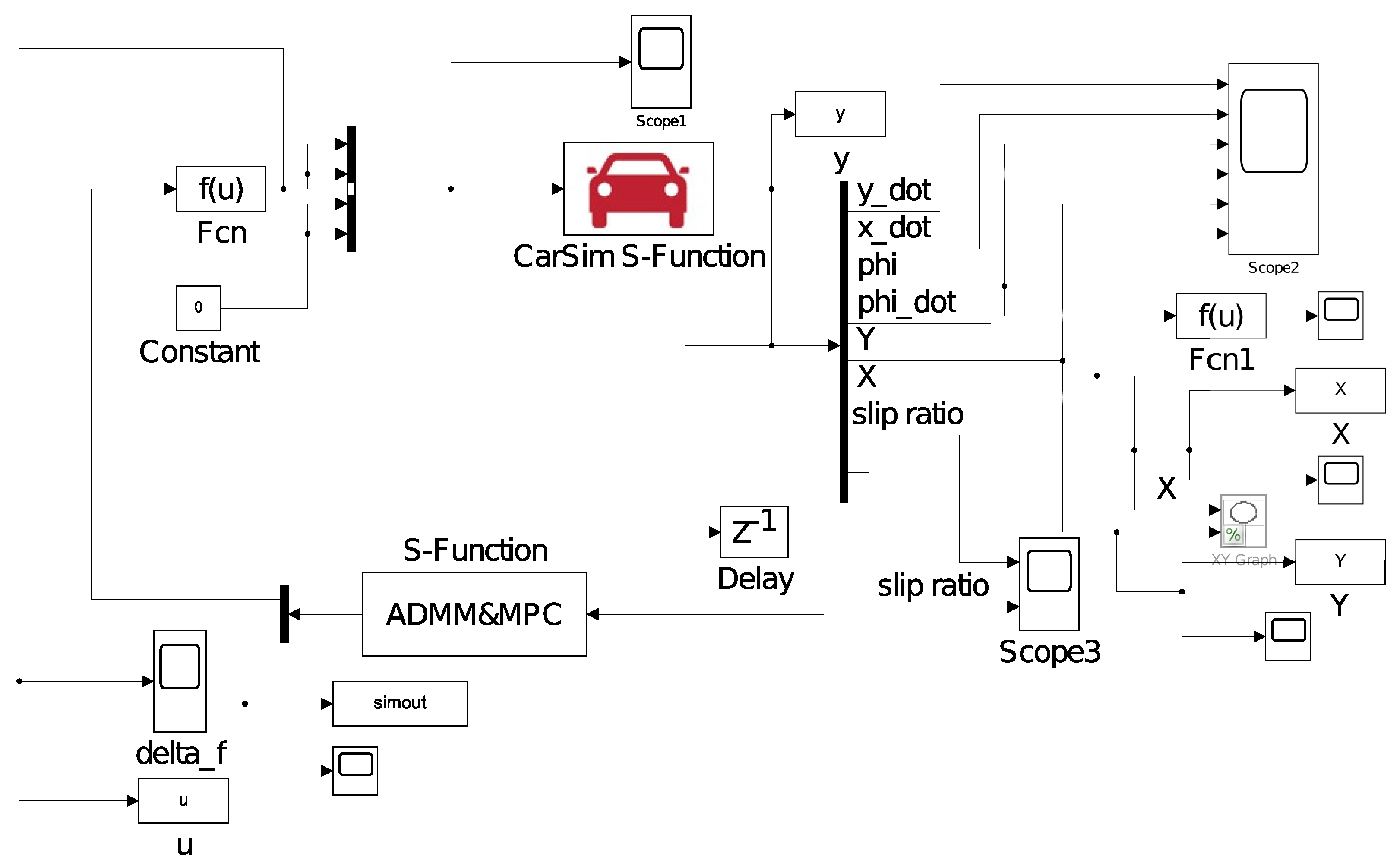
4. Simulation
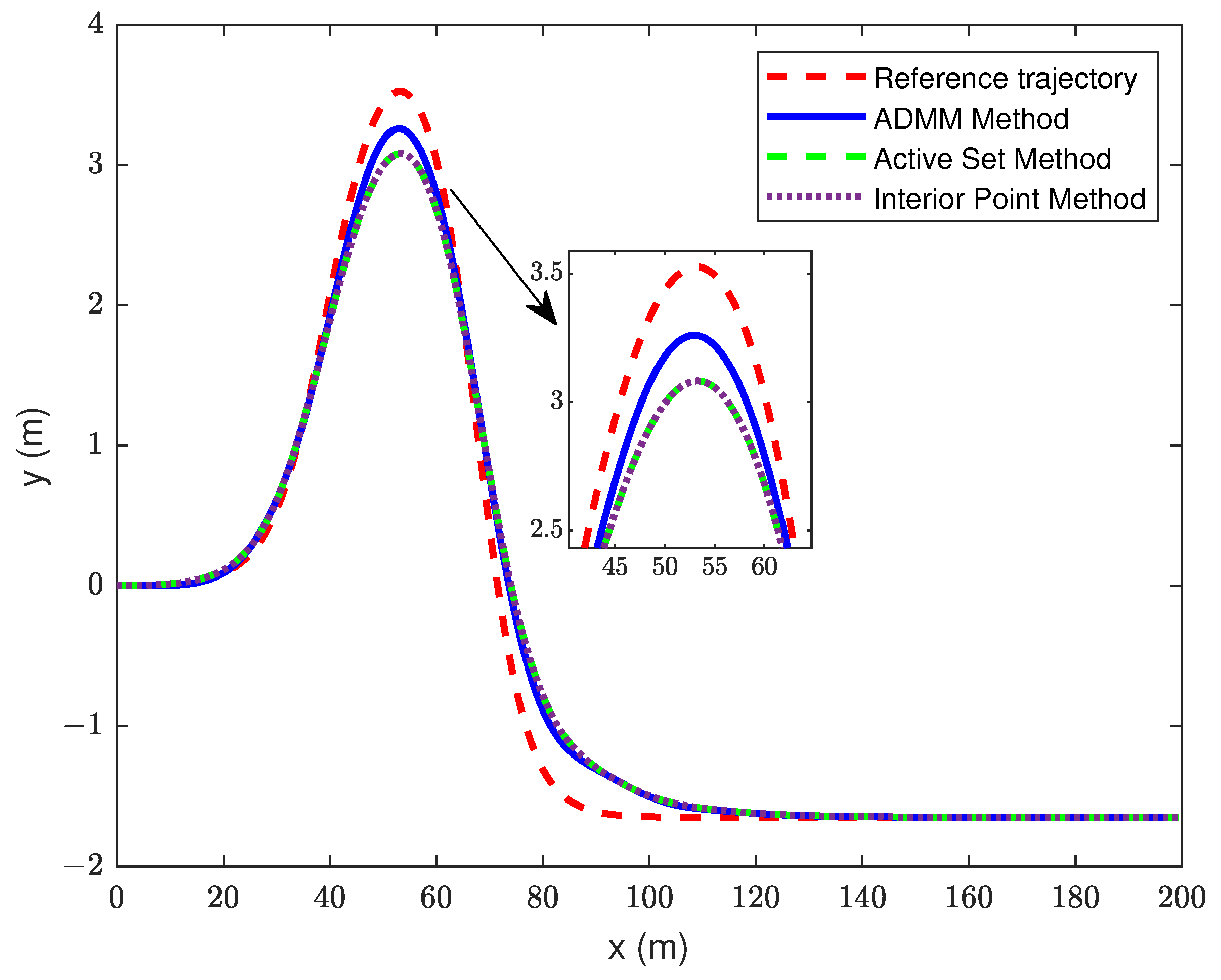
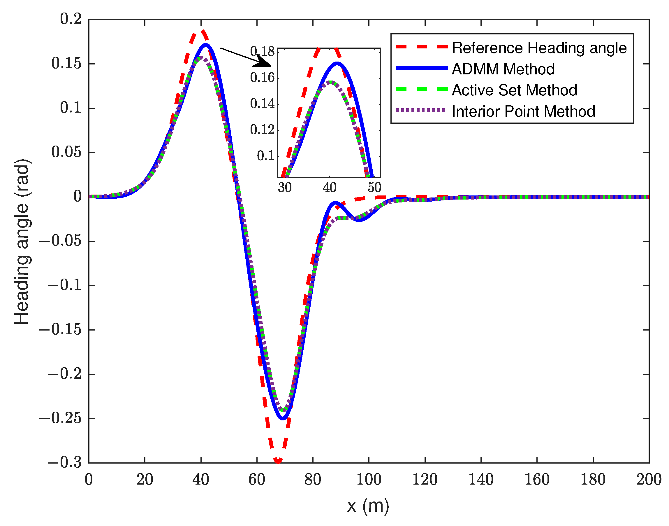
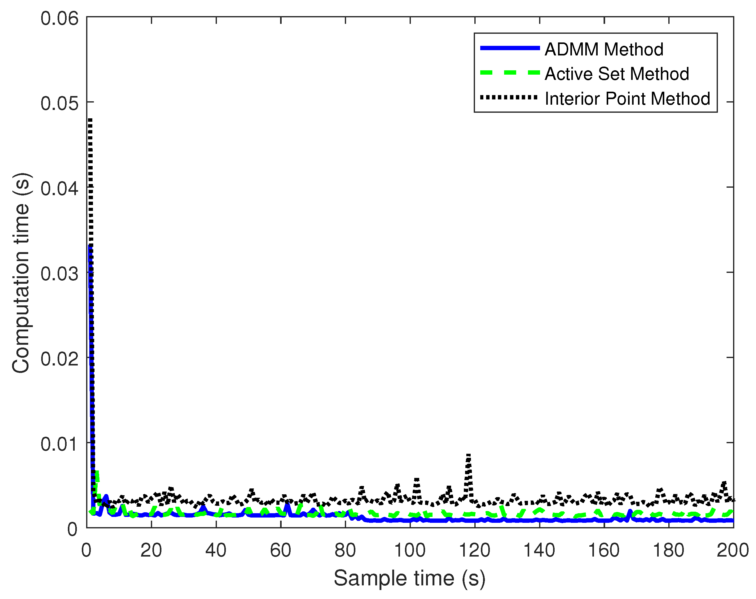
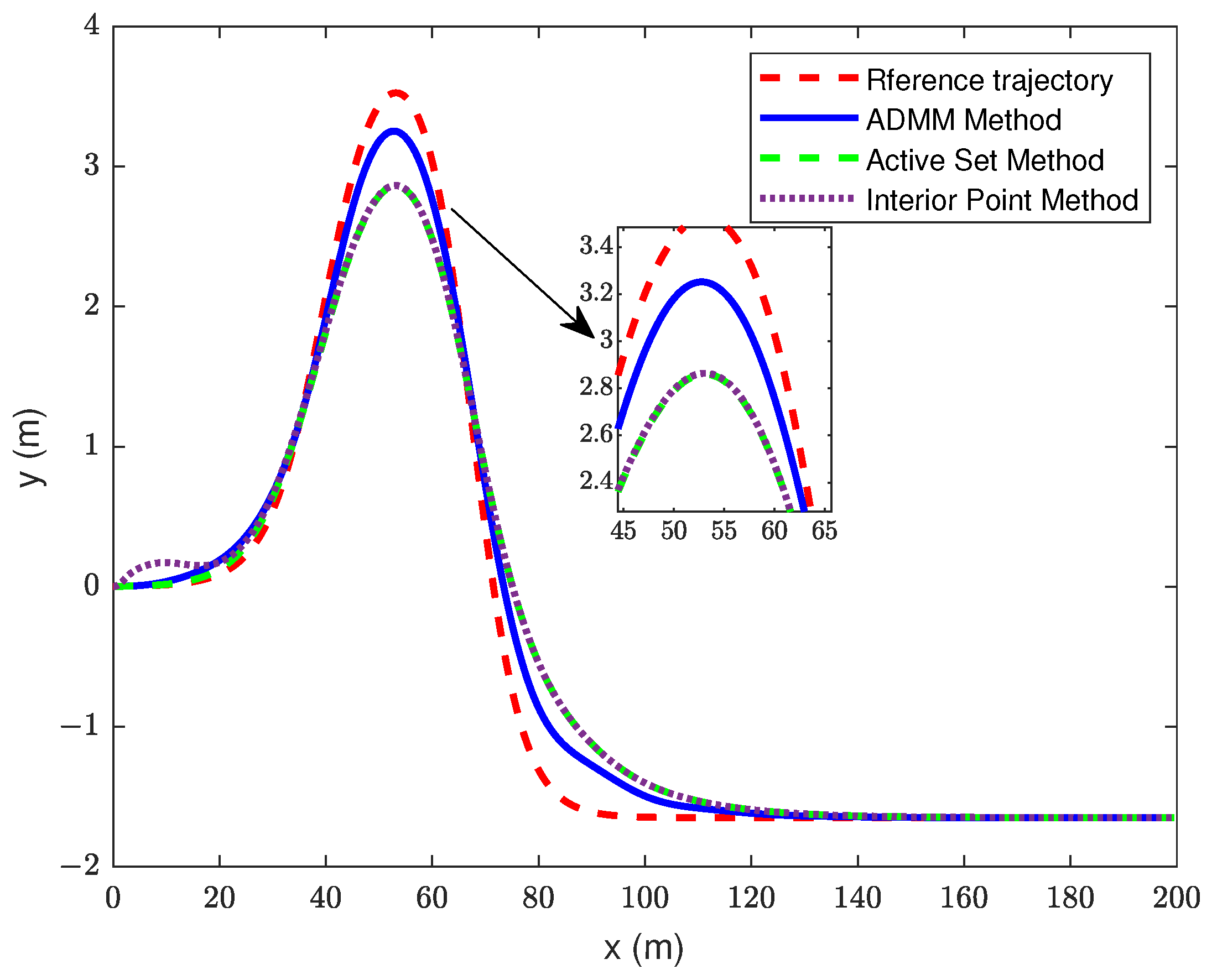
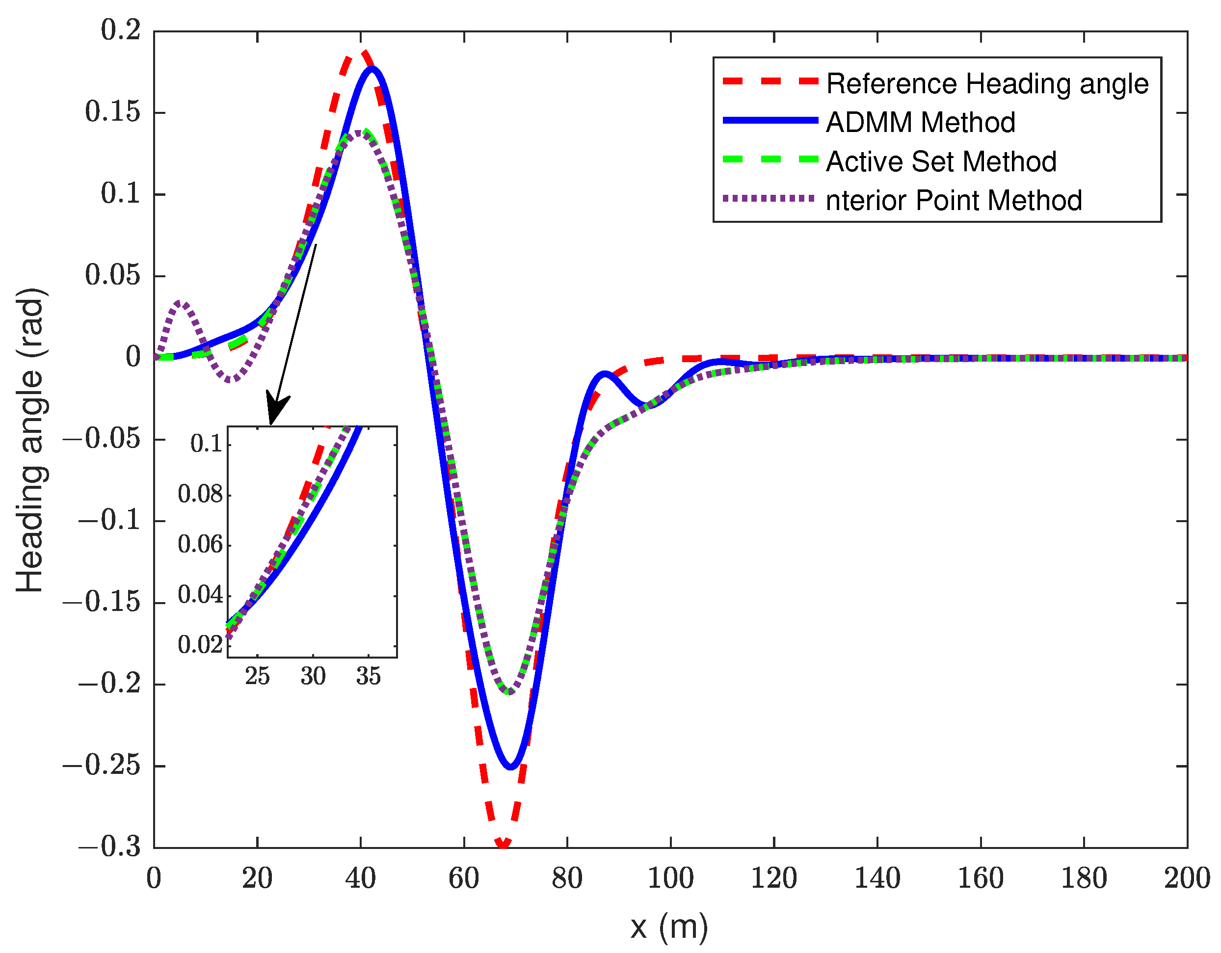
4.1. Comparison of Controllers under the Same Prediction and Control Horizon (, )
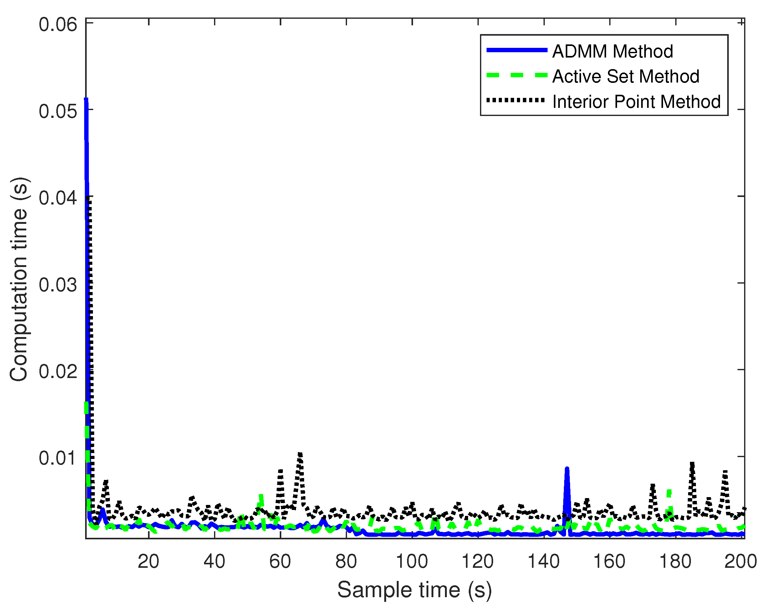
4.2. Comparison of Controllers under Different Control Horizons
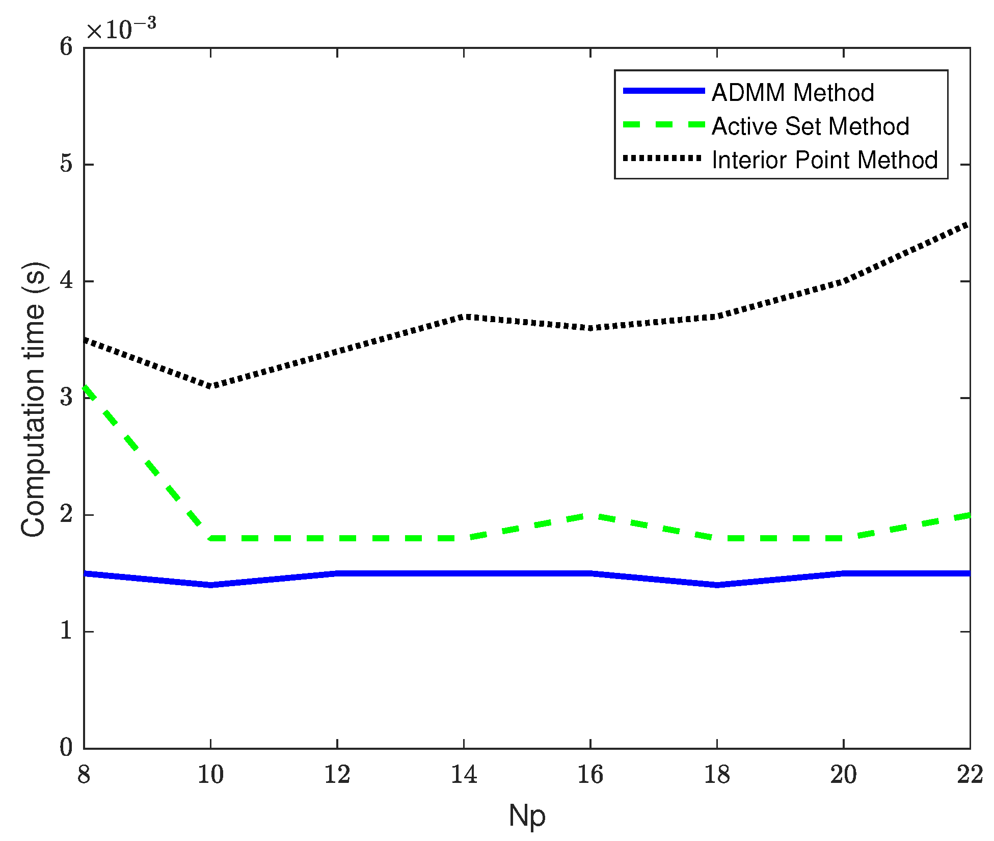
4.3. Comparison of Controller Computation Time as the Prediction Horizon Increases
5. Conclusions
Author Contributions
Funding
Institutional Review Board Statement
Informed Consent Statement
Data Availability Statement
Acknowledgments
Conflicts of Interest
References
- Chen, H.; Guo, L.; Gong, X.; Gao, B.; Zhang, L. Automotive control in intelligent era. Acta Autom. Sin. 2020, 46, 1313–1332. [Google Scholar]
- Yurtsever, E.; Lambert, J.; Carballo, A.; Takeda, K. A survey of autonomous driving: Common practices and emerging technologies. IEEE Access 2020, 8, 58443–58469. [Google Scholar] [CrossRef]
- Sun, C.; Zhang, X.; Zhou, Q.; Tian, Y. A Model Predictive Controller With Switched Tracking Error for Autonomous Vehicle Path Tracking. IEEE Access 2019, 7, 53103–53114. [Google Scholar] [CrossRef]
- Scheffe, P.; Henneken, T.M.; Kloock, M.; Alrifaee, B. Sequential Convex Programming Methods for Real-Time Optimal Trajectory Planning in Autonomous Vehicle Racing. IEEE Trans. Intell. Veh. 2023, 8, 661–672. [Google Scholar] [CrossRef]
- Shi, P.; Long, L.; Xuan, N.; Yang, A. Intelligent Vehicle Path Tracking Control Based on Improved MPC and Hybrid PID. IEEE Access 2022, 10, 94133–94144. [Google Scholar]
- Li, S.; Wang, G.; Zhang, B.; Yu, Z.; Cui, G. Vehicle Yaw Stability Control at the Handling Limits Based on Model Predictive Control. Int. J. Automot. Technol. 2020, 21, 361–370. [Google Scholar] [CrossRef]
- Qi, L.; Jiao, X.; Wang, Z. Trajectory Tracking Control of Intelligent Vehicle Based on DDPG Method of Reinforcement Learning. China J. Highw. Transp. 2021, 34, 335–348. [Google Scholar]
- Ducajú, J.M.S.; Llobregat, J.J.S.; Cuenca, Á.; Tomizuka, M. Autonomous Ground Vehicle Lane-Keeping LPV Model-Based Control: Dual-Rate State Estimation and Comparison of Different Real-Time Control Strategies. Sensors 2021, 21, 1531. [Google Scholar] [CrossRef]
- Kanchwala, H.; Bezerra, V.I.; Aouf, N. Cooperative path-planning and tracking controller evaluation using vehicle models of varying complexities. Proc. Inst. Mech. Eng. Part C J. Mech. Eng. Sci. 2020, 235, 2877–2896. [Google Scholar] [CrossRef]
- Choi, W.; Nam, H.; Kim, B.; Ahn, C. Model Predictive Control for Evasive Steering of Autonomous Vehicle. Int. J. Automot. Technol. 2019, 20, 1033–1042. [Google Scholar]
- Khan, S.; Guivant, J.; Li, X. Design and experimental validation of a robust model predictive control for the optimal trajectory tracking of a small-scale autonomous bulldozer. Robot. Auton. Syst. 2022, 147, 103903. [Google Scholar] [CrossRef]
- Jiang, C.; Zhai, J.; Tian, H.; Wei, C.; Hu, J. Approximated Long Horizon MPC with Hindsight for Autonomous Vehicles Path Tracking. In Proceedings of the 2020 3rd International Conference on Unmanned Systems (ICUS), Harbin, China, 27–28 November 2020; pp. 696–701. [Google Scholar]
- Mata, S.; Zubizarreta, A.; Pinto, C. Robust tube-based model predictive control for lateral path tracking. IEEE Trans. Intell. Veh. 2019, 4, 569–577. [Google Scholar] [CrossRef]
- Tang, Z.; Xu, X.; Wang, F. Coordinated control for path following of two-wheel independently actuated autonomous ground vehicle. IET Intell. Transp. Syst. 2019, 13, 628–635. [Google Scholar] [CrossRef]
- Wang, H.; Liu, B.; Ping, X.; An, Q. Path Tracking Control for Autonomous Vehicles Based on an Improved MPC. IEEE Access 2019, 7, 161064–161073. [Google Scholar] [CrossRef]
- Pereira, G.C.; Wahlberg, B.; Pettersson, H.; Mårtensson, J. Adaptive reference aware MPC for lateral control of autonomous vehicles. Cont. Eng. Pract. 2023, 132, 105403. [Google Scholar] [CrossRef]
- Nan, J.; Shang, B.; Deng, W.; Ren, B.; Liu, Y. MPC-based Path Tracking Control with Forward Compensation for Autonomous Driving. IFAC-PapersOnLine 2021, 54, 443–448. [Google Scholar] [CrossRef]
- Tang, X.; Shi, L.; Wang, B.; Cheng, A. Weight Adaptive Path Tracking Control for Autonomous Vehicles Based on PSO-BP Neural Network. Sensors 2023, 23, 412. [Google Scholar] [CrossRef]
- Domina, Á.; Tihanyi, V. Model Predictive Controller Approach for Automated Vehicle’s Path Tracking. Sensors 2023, 23, 6862. [Google Scholar] [CrossRef]
- Tan, Q.; Dai, P.; Zhang, Z.; Katupitiya, J. MPC and PSO Based Control Methodology for Path Tracking of 4WS4WD Vehicles. Appl. Sci. 2018, 8, 1000. [Google Scholar] [CrossRef]
- Xu, F.; Zhang, J.; Hu, Y.; Qu, T.; Qu, Y.; Liu, Q. Lateral and longitudinal coupling real-time predictive controller for intelligent vehicle path tracking. J. Jilin Univ. (Eng. Technol. Ed.) 2021, 51, 2287–2294. [Google Scholar]
- Shekhar, R.C.; Manzie, C. Optimal move blocking strategies for model predictive control. Automatica 2015, 61, 27–34. [Google Scholar] [CrossRef]
- Leng, Y.; Zhao, S. Explicit Model Predictive Control for Intelligent Vehicle Lateral Trajectory Tracking. J. Syst. Simul. 2021, 33, 1177–1187. [Google Scholar]
- Kayacan, E.; Kayacan, E.; Ramon, H.; Saeys, W. Learning in Centralized Nonlinear Model Predictive Control: Application to an Autonomous Tractor-Trailer System. IEEE Trans. Control Syst. Technol. 2014, 23, 197–205. [Google Scholar] [CrossRef]
- Pas, P.; Schuurmans, M.; Patrinos, P. Alpaqa: A matrix-free solver for nonlinear MPC and large-scale nonconvex optimization. In Proceedings of the 2022 European Control Conference (ECC), London, UK, 12–15 July 2022; pp. 417–422. [Google Scholar]
- Zhou, B.; Su, X.; Yu, H.; Guo, W.; Zhang, Q. Research on Path Tracking of Articulated Steering Tractor Based on Modified Model Predictive Control. Agriculture 2023, 13, 871. [Google Scholar] [CrossRef]
- Ju, F.; Zong, Y.; Zhuang, W.; Wang, Q.; Wang, L. Real-Time NMPC for Speed Planning of Connected Hybrid Electric Vehicles. Machines 2022, 10, 1129. [Google Scholar] [CrossRef]
- Bai, G.; Liu, L.; Meng, Y.; Liu, S. Real-time path tracking of mobile robot based on nonlinear model predictive control. J. Agric. Mach. 2020, 51, 47–52+60. [Google Scholar]
- Alcalá, E.; Puig, V.; Quevedo, J. LPV-MPC Control for Autonomous Vehicles. IFAC-PapersOnLine 2019, 52, 106–113. [Google Scholar] [CrossRef]
- Cheng, Z.; Ma, J.; Zhang, X.; Lee, T. Semi-Proximal ADMM for Model Predictive Control Problem with Application to a UAV System. In Proceedings of the 2020 20th International Conference on Control, Automation and Systems (ICCAS), Busan, Republic of Korea, 13–16 October 2020; pp. 82–87. [Google Scholar]
- Li, X.; Tyagi, A. Block-Active ADMM to Minimize NMF with Bregman Divergences. Sensors 2023, 23, 7229. [Google Scholar] [CrossRef]
- Toyoda, M.; Tanaka, M. An analysis of hot-started ADMM for linear MPC. IET Control. Theory Appl. 2021, 15, 1999–2016. [Google Scholar] [CrossRef]
- Hong, M.; Lou, Z.; Razaviyayn, M. Convergence analysis of alternating direction method of multipliers for a family of nonconvex problems. In Proceedings of the 2015 IEEE International Conference on Acoustics, Speech and Signal Processing (ICASSP), South Brisbane, QLD, Australia, 19–24 April 2015; pp. 3836–3840. [Google Scholar]
- Ma, J.; Cheng, X.; Zhang, X.; Tomizuka, M.; Lee, T. Alternating Direction Method of Multipliers for Constrained Iterative LQR in Autonomous Driving. IEEE Trans. Intell. Transp. Syst. 2022, 23, 23031–23042. [Google Scholar] [CrossRef]
- Vroemen, B.; Essen, V.; Steenhoven, V.A.; Kok, J.J. Nonlinear model predictive control of a laboratory gas turbine installation. J. Eng. Gas Turbine Power 1999, 121, 629–634. [Google Scholar] [CrossRef]
- Lau, M.S.K.; Yue, S.; Ling, K.; Maciejowski, J.M. A comparison of interior point and active set methods for FPGA implementation of model predictive control. In Proceedings of the European Control Conference (ECC), Budapest, Hungary, 23–26 August 2009; pp. 156–161. [Google Scholar]
- Shahzad, A.; Kerrigan, E.C.; Constantinides, G.A. A warm-start interior-point method for predictive control. In Proceedings of the UKACC International Conference on Control 2010, Coventry, UK, 7–10 September 2010; pp. 1–6. [Google Scholar]
- Lin, X.; Tang, Y.; Zhou, B. Improved Model Predictive Control Path Tracking Strategy Based an Online Updating Algorithm with Cosine Similarity and a Horizon Factor. IEEE Trans. Intell. Transp. Syst. 2022, 23, 12429–12438. [Google Scholar] [CrossRef]
- Shan, R.; Li, Q.; He, F.; Feng, M.; Guan, T. Model predictive control based on ADMM for aero-engine. J. Beijing Univ. Aeronaut. Astronaut. 2019, 6, 8. [Google Scholar]


| Parameters | Value | Unit |
|---|---|---|
| vehicle weight | 1723 | kg |
| lateral moment of inertia | 4331.6 | kg · m |
| roll moment of inertia | 4175 | kg · m |
| distance from front axle to center of mass | 1.232 | m |
| distance from rear axle to center of mass | 1.468 | m |
| front track width | 1.480 | m |
| front and rear axle roll stiffness | 2328/2653 | N · m/rad |
| front and rear axle roll damping | 47,298/37,311 | N · m/rad |
| front wheel lateral stiffness | 66,900 | N/rad |
| rear wheel lateral stiffness | 61,900 | N/rad |
| wheel rotational inertia | 0.9 | kg · m |
| rolling radius of the wheel | 0.353 | m |
| Method | ADMM | Active Set Method | Interior Point Method |
|---|---|---|---|
| Average computation time (s) | 0.0013 | 0.0020 | 0.0035 |
| Method | ADMM | Active Set Method | Interior Point Method |
|---|---|---|---|
| Average computation time (s) | 0.0015 | 0.0018 | 0.0038 |
| ADMM Computation Time (s) | Active Set Method Computation Time (s) | Interior Point Method Computation Time (s) | |
|---|---|---|---|
| 8 | 0.0015 | 0.0031 | 0.0035 |
| 10 | 0.0014 | 0.0018 | 0.0031 |
| 12 | 0.0015 | 0.0018 | 0.0034 |
| 14 | 0.0015 | 0.0018 | 0.0037 |
| 16 | 0.0015 | 0.0020 | 0.0036 |
| 18 | 0.0014 | 0.0018 | 0.0037 |
| 20 | 0.0015 | 0.0018 | 0.0040 |
| 22 | 0.0015 | 0.0020 | 0.0045 |
Disclaimer/Publisher’s Note: The statements, opinions and data contained in all publications are solely those of the individual author(s) and contributor(s) and not of MDPI and/or the editor(s). MDPI and/or the editor(s) disclaim responsibility for any injury to people or property resulting from any ideas, methods, instructions or products referred to in the content. |
© 2023 by the authors. Licensee MDPI, Basel, Switzerland. This article is an open access article distributed under the terms and conditions of the Creative Commons Attribution (CC BY) license (https://creativecommons.org/licenses/by/4.0/).
Share and Cite
Dong, D.; Ye, H.; Luo, W.; Wen, J.; Huang, D. Fast Trajectory Tracking Control Algorithm for Autonomous Vehicles Based on the Alternating Direction Multiplier Method (ADMM) to the Receding Optimization of Model Predictive Control (MPC). Sensors 2023, 23, 8391. https://doi.org/10.3390/s23208391
Dong D, Ye H, Luo W, Wen J, Huang D. Fast Trajectory Tracking Control Algorithm for Autonomous Vehicles Based on the Alternating Direction Multiplier Method (ADMM) to the Receding Optimization of Model Predictive Control (MPC). Sensors. 2023; 23(20):8391. https://doi.org/10.3390/s23208391
Chicago/Turabian StyleDong, Ding, Hongtao Ye, Wenguang Luo, Jiayan Wen, and Dan Huang. 2023. "Fast Trajectory Tracking Control Algorithm for Autonomous Vehicles Based on the Alternating Direction Multiplier Method (ADMM) to the Receding Optimization of Model Predictive Control (MPC)" Sensors 23, no. 20: 8391. https://doi.org/10.3390/s23208391