Estimation of Reference Evapotranspiration in a Semi-Arid Region of Mexico

Abstract

Reference evapotranspiration (ET₀) is the first step in calculating crop irrigation demand, and numerous methods have been proposed to estimate this parameter. FAO-56 Penman–Monteith (PM) is the only standard method for defining and calculating ET₀. However, it requires radiation, air temperature, atmospheric humidity, and wind speed data, limiting its application in regions where these data are unavailable; therefore, new alternatives are required. This study compared the accuracy of ET₀ calculated with the Blaney–Criddle (BC) and Hargreaves–Samani (HS) methods versus PM using information from an automated weather station (AWS) and the NASA-POWER platform (NP) for different periods. The information collected corresponds to Module XII of the Lagunera Region Irrigation District 017, a semi-arid region in the North of Mexico. The HS method underestimated the reference evapotranspiration (ET₀) by 5.5% compared to the PM method considering the total ET₀ of the study period (26 February to 9 August 2021) and yielded the best fit in the different evaluation periods (daily, 5-day mean, and 5-day cumulative); the latter showed the best values of inferential parameters. The information about maximum and minimum temperatures from the NP platform was suitable for estimating ET₀ using the HS equation. This data source is a suitable alternative, particularly in semi-arid regions with limited climatological data from weather stations.

1. Introduction

Evapotranspiration (ET) is the sum of transpiration through the plant canopy and evaporation from the soil, plant, and free surface water [1,2]. ET is the most significant component of the hydrological cycle [1,3], due to which its estimation is of common interest in climatological, hydrological, forestry, and agricultural studies [4]. This last area ET is a fundamental variable for calculating water requirements, making efficient use of water in crop production [5]. ET can be measured directly using weighing lysimeters or by measuring the net flux of water vapor between the surface and the surrounding atmosphere using micrometeorological methods [6], which depend on the energy balance of the canopy and include the energy balance of Bowen’s relation, eddy covariance, and the use of scintillometers [7].

Crop evapotranspiration (ET_C) is a crucial aspect of the water balance in agricultural areas. To estimate it, the most accessible method is to estimate reference evapotranspiration (ET₀) and then pair it with crop and soil coefficients [8]. Reference evapotranspiration (ET₀) is the evapotranspiration rate of a hypothetical reference crop (grass or alfalfa) with a height of 0.12 m, a fixed surface resistance of 70 s m⁻¹, and an albedo of 0.23, homogeneous, well-watered, free from diseases and pests, growing vigorously, and providing complete shade to the soil [9,10,11]. ET₀ measures atmospheric evaporation demand regardless of crop type, development, and management practices [12,13]. This variable is affected only by climatic factors [14] and can be calculated from meteorological data [10].

Estimating ET₀ is the first step in designing, planning, and managing different irrigation systems [15,16]. In addition, it is relevant for calculating crop water requirements [17,18]. This parameter is the backbone of the agronomic design of any irrigation system, facilitates its operation (irrigation schedule and shifts), and allows the planning of water resource management in a basin [19] or an irrigation district. Therefore, its accurate estimation is essential in water management, particularly in arid and semi-arid areas where water is scarce [20].

Given its importance, and the climate’s temporal and spatial variability, many models to estimate ET₀ have been proposed. In general, the models available in the published literature can be broadly classified as follows: (1) fully physically based models on a combination of energy balance and mass transfer; (2) semi-physical models based on temperature, radiation, and evaporation data; and (3) black-box models based on artificial neural networks, empirical relationships, and genetic and fuzzy algorithms [21,22].

Due to its practicality, many empirical equations have been developed from field experiments and those based on theoretical approaches [19]. These methods include the evaporimeter tank and empirical equations, including the complete physical model (FAO-56 Penman–Monteith), the equation based on temperature (Blaney–Criddle, Thornthwaite, and Turc), and the one based on temperature and radiation (Hargreaves, Jensen–Haise, Priestley–Taylor, and FAO Radiation), among others [21].

The UN Food and Agriculture Organization (FAO) recommends the Penman–Monteith standard method described in the FAO-56 Manual because it can be used in arid, temperate, and tropical areas [23]. Furthermore, this standardized method is more accurate than the standard proposed by the American Society of Civil Engineers (ASCE), ASCE-PM, when estimating daily ET₀; both ways were compared with lysimetric measurements [24]. However, this method requires various meteorological input variables (temperature, solar radiation, relative humidity, and wind speed), which restrains its widespread use [25]. Therefore, its usefulness is limited in regions with no meteorological stations or a shortage of input data [26], which are usually unavailable with the required frequency and quality [27]. The other equations can be used in regions with very little climatological information, such as the case of Hargreaves–Samani (HS) and Blaney–Criddle (BC) equations, which are the most common ones [28,29,30] and only require temperature as an input variable [31].

The accuracy of the HS and BC equations has been evaluated by several authors, comparing their results with the FAO-56 Penman–Monteith (PM) reference method; HS was the equation that attained the best fit in semi-arid regions [32,33]. Other authors state that the HS method works well in most climatic regions, except for wet areas where it tends to overestimate ET₀ [16,34,35,36]. Since HS was developed empirically based on data from arid to subhumid environments, it may not fit well to conditions markedly different from those considered for its calibration, as is the case of wet climates [16]. On the other hand, the HS method underestimates ET₀ for dry and windy areas because it does not include wind and is seemingly more accurate when applied for 5- to 7-day averages than for daily time scales [37,38]. However, despite a reasonably good performance of the HS equation in most applications, particularly irrigation planning, several authors have attempted to either recalibrate the HS coefficients or parameters [36,39] or modify the equation itself [40,41], aiming to improve its performance.

Reanalysis data or gridded meteorological data are an alternate source of information that can be used to estimate ET₀ [42,43,44]. It is available on different platforms: National Aeronautics and Space Administration—Prediction of Worldwide Energy Resource (NASA-POWER) [27,45], Global Land Data Assimilation System (GLDAS) [46], Climate Forecast System ver. 2 (CFSv2) [47], North American Land Data Assimilation System (NLDAS) [48], and National Digital Forecast Database (NDFD) [49]. These global or regional platforms provide data with higher spatial and temporal resolution [27]. However, it should be noted that higher spatial resolution does not necessarily imply higher precision [50]. The NASA-POWER platform (NP) is the most widely used to estimate ET₀ [51,52,53]. NP provides daily information on air temperature, precipitation, relative humidity, radiation, wind direction, and speed; it is free and easily accessible. This information is grouped into three different spatial conditions: for a single point, with time series data available based on registered geographic coordinates chosen by the user; at the regional level, in a time series dataset based on a bounding box of user-determined geographic coordinates; and globally, with climate averages worldwide [54]. Despite the wide availability of information and ease of access, evaluating and validating said NP climate information with in situ weather stations in the area of interest is essential for local bias correction and to improve accuracy [45].

This study aims to compare the accuracy of ET₀ calculated with the BC and HS methods relative to the FAO-56 Penman–Monteith (PM) reference method, with data recorded by an automated weather station (AWS) and temperature data (maximum and minimum) from the NASA–POWER platform (NP), for different calculation periods.

2. Materials and Methods

2.1. Study Area and Data Collection

The climatic variables to calculate ET₀ with empirical equations were recorded with a wireless Davis Vantage Pro 2 Plus AWS (Davis Instruments Company, Hayward, CA, USA); it has a console that allows viewing of all meteorological variables simultaneously [55], with a 30-min update frequency.

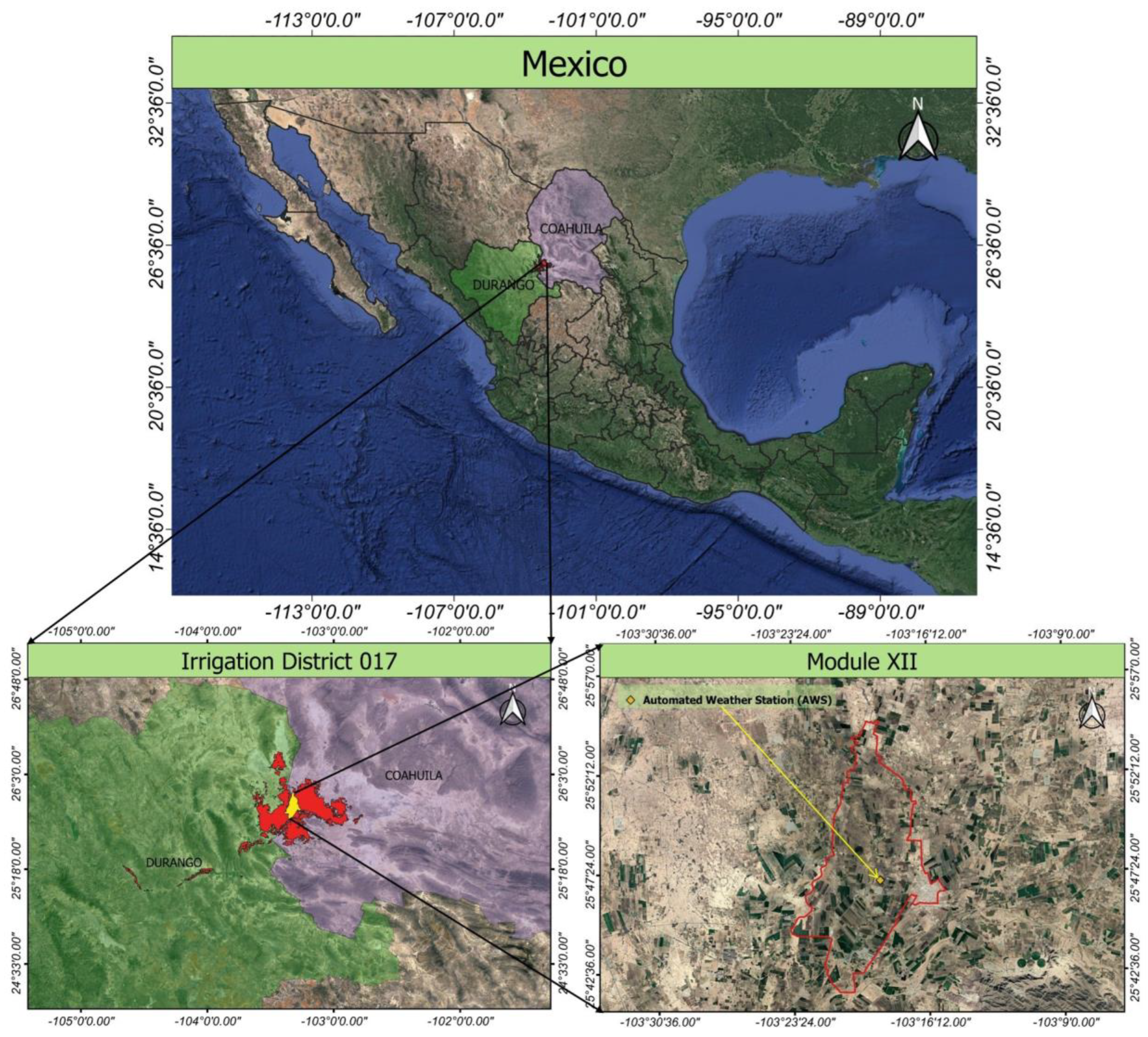
The AWS belongs to Centro Nacional de Investigación Disciplinaria en Relación Agua, Suelo, Planta, Atmósfera (National Center for Disciplinary Research on Water, Soil, Plant, Atmosphere; CENID RASPA) of Instituto Nacional de Investigaciones Forestales, Agrícolas y Pecuarias (National Institute of Forestry, Agricultural, and Livestock Research; INIFAP), within the facilities of an agricultural production unit located at Module XII of the Lagunera Region Irrigation District 017, at 1110 m a.s.l. and coordinates 25°47′00.32″ N, 103°18′46.54″ W (Figure 1).

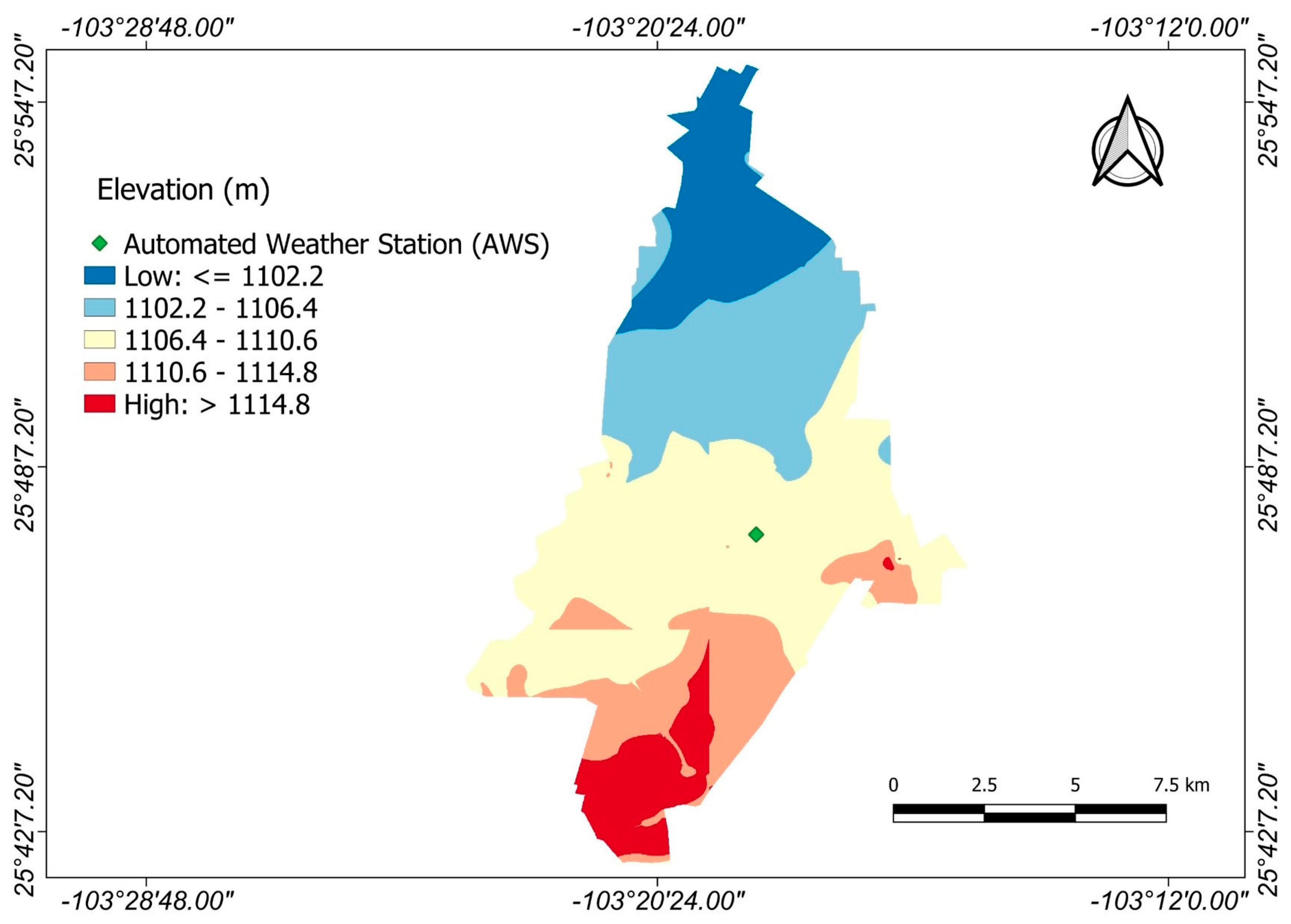
Module XII covers an area of 14,276.7 hectares with an elevation range of 1102 to 1114 m [56]. The slope of the area is gentle, at around 0.06%. It is oriented from south to north, with the southern part being the highest, as shown in Figure 2.

Based on data gathered from Series VII of INEGI (2018) [57], it is estimated that the study area is primarily used for irrigated agriculture, with 89.3% of its surface area dedicated to this use. Human settlements make up 8.7% of the area, while the remaining 2% is used for other purposes (

Table 1. Land use and vegetation of the study area INEGI-Series VII (2018).

Land Use	Code	Surface (ha)	Coverage (%)
Human Settlements	AH	1240.1	8.69
Barren Land	DV	15.6	0.11
Annual and Semi-permanent Irrigated Agriculture	RAS	10,166.6	71.21
Permanent Irrigated Agriculture	RP	63.0	0.44
Semi-permanent Irrigated Agriculture	RS	2521.3	17.66
Microphyllous Desert Scrub with Secondary Shrub Vegetation	Vsa/MDM	237.1	1.66
Halophilous Xerophytic Vegetation with Secondary Shrub Vegetation	Vsa/VH	32.9	0.23
Total		14,276.7	100.00

).

The meteorological information used was daily averages for the period between 26 February (Julian day 57) and 9 August (Julian day 221) 2021 (n = 165). In the Lagunera Region Irrigation District 017, the main crops of the spring–summer cycle are grown in this period, including forage corn.

In addition, the meteorological variables were downloaded from the NP climate website (National Aeronautics and Space Administration—Prediction of Worldwide Energy Resource; https://power.larc.nasa.gov, accessed on 5 October 2022). This website collects information from various sources: data recorded on-site, satellite data, wind probes, and assimilated data systems [27].

The NNP weather data are based on a single assimilation model named GMAO (Global Modeling and Assimilation Office), starting from the MERRA-2 (Modern Era Retrospective-Analysis for Research and Applications) reanalysis dataset and the GEOS (Goddard Earth Observation System) data processing system [58,59]. Solar radiation is derived from the GEWEX SRB (Global Energy and Water Exchanges Project Surface Radiation Budget) project [60,61].

The horizontal resolution of the NP meteorological data source corresponds to a ½° × 5/8° latitude/longitude grid, and the solar data sources come from a 1° × 1° latitude/longitude grid. The current version no longer reassigns data to a common grid; once the data are processed and filed, they are available through the NP service package. The meteorological data is derived from NASA’s GMAO MERRA-2 and GEOS 5.12.4 FP-IT. The NP platform team processes GEOS data daily and combines them with MERRA-2 data, producing daily time series that yield low-latency products usually available in approximately two days (real-time). Energy flow data (solar irradiance, thermal IR, and cloud properties) derive from NASA’s GEWEX SRB Release 4-Integrated Product (R4-IP) file and CERES SYNIdeg and FLASHFlux projects. These data are processed daily and added to the daily time series, issuing products after approximately 4 days, almost in real-time [62].

The main features of the NP system database are shown in

Table 2. Features of the NASA-POWER (NP) system information.

Parameter	Feature
Data period	1981 to date
Geographic range	Global
Download format	ASCII, CSV, GeoJSON, and NetCDF
Temporal resolution	Daily
Spatial resolution	0.5° × 0.5° (55.56 km × 55.56 km cell) for temperature (T), relative humidity (RH), and wind speed ($u_2$). 1.0° × 1.0° for solar radiation and extraterrestrial solar radiation data.
Delayed data availability	Approximately two days for temperature, relative humidity, and wind speed, and five days for solar radiation data.

. The AWS is situated near the center of Module XII (Figure 2) and aligns with the center of the NP platform cell. This suggests that one cell encompasses the entire study area’s surface.

2.2. ET₀ Estimation with Empirical Equations

ET₀ was estimated through three empirical equations with different information requirements: an equation based on a complete physical model (PM); another on temperature and solar radiation (HS); and the last one on temperature, relative humidity, and wind speed (BC).

2.2.1. FAO-56 Penman–Monteith Method (ET₀-PM)

ET₀ was estimated daily with the FAO-56 Penman–Monteith method using Equation (1) [22,63]; this method is useful for arid, temperate, and tropical zones [19,22].

$${ET}_{0-PM}=\frac{0.408∆\left(R_n-G\right)+\gamma \frac{900}{T+273}{u}_2\left(e_s-e_a\right)}{∆+\gamma \left(1+0.34u_2\right)},$$

(1)

where $R_n$ is the net radiation at the reference crop surface (MJ m⁻² d⁻¹); $G$ is the soil heat flux density (MJ m⁻² d⁻¹); $u_2$ is the wind speed at 2 m height (m s⁻¹); $e_s$ is the saturation vapor pressure (kPa); $e_a$ is the actual vapor pressure (kPa); $e_s-e_a$ is the vapor pressure deficit (kPa); $∆$ is the slope of the vapor saturation pressure curve (kPa °C⁻¹); $T$ is the mean daily air temperature at 2 m height (°C); and $\gamma$ is the psychrometric constant (kPa °C⁻¹). For daily time intervals, $G$ values are relatively small, and therefore, this term was not included [22].

2.2.2. Hargreaves–Samani Method (ET₀-HS)

The Hargreaves–Samani method estimates ET₀ based on temperature data only (Equation (2)) [64]. This equation was developed for semi-arid zones and is useful when solar radiation data are not available; however, as it is based on a few variables, its accuracy should be evaluated at the regional and local levels [65].

$${ET}_{0-HS}=K_H\left(T+K_T\right)R_0\times { \left(T_{max}-T_{min}\right)}^{A_H},$$

(2)

where $T$ is the mean daily air temperature (°C); $R_0$ is the extraterrestrial solar radiation (from tables, mm d⁻¹); $T_{max}$ is the maximum daily air temperature (°C); $T_{min}$ is the minimum daily air temperature (°C); $K_H$ and $K_T$ are the empirical calibration parameters; and $A_H$ is a Hargreaves’ empirical exponent. This study used the original values proposed by Hargreaves and Samani [64]: $K_H$= 0.0023, $K_T$ = 17.78, and $A_H$ = 0.5.

2.2.3. Blaney–Criddle Method (ET₀-BC)

The meteorological variables required to apply the Blaney–Criddle method are air temperature, relative humidity, and daytime wind speed (Equation (3) [66].

$${ET}_{0-BC}=a+b\left[p\left(0.46\times T+8.13\right)\right],$$

(3)

where $a$ and $b$ are climatic calibration coefficients calculated with Equations (4) and (5), respectively; $p$ is the mean annual percentage of daytime hours (value from tables, decimal); and $T$ is the mean air temperature at 2 m height (°C).

$$a=0.0043\times {RH}_{min}-\frac{n}{N}-1.41,$$

(4)

where ${RH}_{MIN}$ is the minimum relative humidity (%); $\frac{n}{N}$ is the ratio between theoretical and actual sunlit hours (value from tables, decimal).

$$b=0.082-0.0041\left({RH}_{min}\right)+1.07\left(\frac{n}{N}\right)+0.066\left(u_2\right)-0.006\left({RH}_{min}\right)\left(\frac{n}{N}\right)-0.0006\left({RH}_{min}\right)\left(u_2\right),$$

(5)

where $u_2$ is the mean daily wind speed at 2 m height (m s⁻¹).

2.3. Inferential Evaluation Parameters

Table 3. Equations and optimal values of inferential parameters.

Parameter	Equation		Optimal Value
Coefficient of Determination ($R^2$)	$R^2=\frac{{\left[\sum _{i=1}^n\left(E_i-\overline{E}\right)\left(O_i-\overline{O}\right)\right]}^2}{\sum _{i=1}^n{\left(E_i-\overline{E}\right)}^2{\sum }_{i=1}^n{\left(O_i-\overline{O}\right)}^2}$	(6)	1
Root Mean Error ($RMSE$)	$RMSE=\sqrt{\frac{{\sum }_{i=1}^n{\left(E_i-O_i\right)}^2}{n}}$	(7)	0
Estimate Error Percentage ($PE$)	$PE=\left|\frac{\overline{E}-\overline{O}}{\overline{O}}\right|\ast 100$	(8)	0
Mean Error Bias ($MBE$)	$MBE=\frac{{\sum }_{i=1}^n\left(E_i-O_{\mathrm{i}}\right)}{n}$	(9)	0
Concordance Index ($d$)	$d=1-\left[\frac{{\sum }_{i=1}^n{\left(E_i-O_i\right)}^2}{{\sum }_{i=1}^n{\left(\left|E_i-\overline{O}\right|+\left|O_i-\overline{O}\right|\right)}^2}\right]$	(10)	1
Correlation coefficient ($r$)	$r=\frac{{\sum }_{i=1}^n\left(\left|O_i-\overline{O}\right|\right)\left(\left|E_i-\overline{E}\right|\right)}{\sqrt{{\sum }_{i=1}^n{\left(O_i-\overline{O}\right)}^2}\sqrt{{\sum }_{i=1}^n{\left(E_i-\overline{E}\right)}^2}}$	(11)	1
Reliability coefficient ($c$)	$c=r\ast d$	(12)	1
Regression coefficient ($b$)	$b=\frac{{\sum }_{i=1}^n{O}_i{E}_i}{{\sum }_{i=1}^n{O_i}^2}$	(13)	1

shows the inferential parameters used for evaluating the empirical equations that estimate ET₀ (HS and BC), considering the PM method as a reference. Likewise, the climatic information of the NP platform was evaluated when calculating ET₀ through the reference method (PM_NP).

In the above equations, $E_i$ is the estimated value using the empirical equation; $O_i$ is the value obtained with the reference method; $\overline{E}$ is the average of estimated values obtained with the empirical equation; $\overline{O}$ is the average of the values obtained with the reference method; and $n$ is the number of observations. The criteria for interpreting the reliability coefficient are cited in [67].

ET₀ was estimated in three different ways with empirical equations (daily, mean, and cumulative) using a total of 165 observations. The mean ET₀ was determined over the 5-day period, as was the cumulative.

3. Results and Discussion

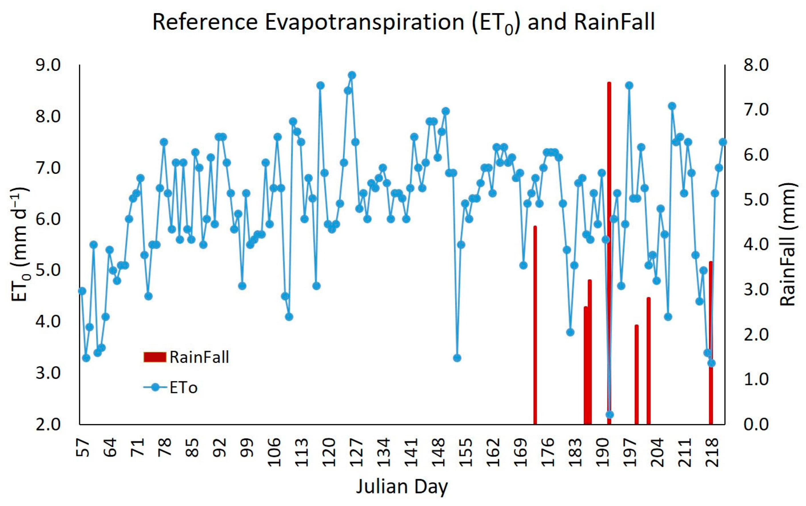
The daily ET₀ calculated by the PM method and with AWS meteorological data (Figure 3) had the peak value (8.8 mm d⁻¹) on Julian day 126 (6 May 2021)—on the same day, a wind speed of 5.0 m s⁻¹ was recorded, which was higher than the average recorded over the study period (2.2 m s⁻¹). On the other hand, the minimum ET₀ (2.2 mm day⁻¹) was recorded on Julian day 192 (11 July 2021)—the day that recorded a solar radiation value of 107.0 W m⁻², lower than the average for the study period (282.8 W m⁻²). This low radiation was due to atypical conditions: high cloudiness (rainfall of 7.6 mm recorded) and high relative humidity (84.5%). Some authors mention that wind speed and solar radiation are the climatic variables with the most significant influence on ET₀ estimates in the study area [27]. Other authors reach the same conclusion when performing a sensitivity analysis in other regions [68,69,70].

3.1. Comparison of ET₀ Estimated by Empirical Equations versus the Reference Method

Table 4. Monthly and total ET₀ estimated by empirical equations and the reference method (FAO-56 Penman–Monteith) during the study period.

Variable	Evaluation Period: 26 February to 9 August 2021
	February	March	April	May	June	July	August	Total
	(n = 3)	(n = 31)	(n = 30)	(n = 31)	(n = 30)	(n = 31)	(n = 9)	(n = 165)
ET0-PM (mm)	11.7	179.0	191.3	214.4	196.7	187.8	49.1	1030.0
ET0-HS (mm)	13.2	154.8	180.8	200.3	195.5	179.6	48.7	972.9
ET0-BC (mm)	12.5	141.3	152.1	171.7	172.2	170.9	48.8	869.5
ET0-PM_NP (mm)	13.4	183.7	204.8	242.7	238.5	203.5	52.3	1138.9

shows the monthly and total ET₀ estimated using the empirical equations and the reference method (PM). Considering the month with the maximum ET₀ (May, with the HS and PM_NP equations and June with the BC method) and the reference method (PM), HS yielded an ET₀ value that was 6.6% lower vs. PM; BC, 12.5% lower; and PM_NP, 13.2% higher. However, considering the month with the minimum ET₀ (February) and the PM method, HS yielded an ET₀ 12.8% higher vs. PM; BC, 6.8% higher; and PM_NP, 14.2% higher. It is observed that HS and BC underestimate ET₀ over most of the study period, consistent with the findings reported by some authors for an agroclimatic region similar to the study area [71].

However, when considering total ET₀ (whole study period) and the PM method, HS recorded an ET₀ value 5.5% lower vs. PM; BC, a value 15.6% lower; and PM_NP, 10.6% higher; therefore, HS was the equation that yielded values closest to the PM method. This is because HS considers temperature and radiation as the main energy sources that promote evapotranspiration [9,27].

The results in Table 4 indicate an overestimation of ET₀ relative to the value obtained with the PM_NP method during the study period. The magnitude of this overestimation is related to the accuracy of each variable and has been reported only when using NP (NASA-POWER) data and the PM method [52,53,72].

Table 5. Relationship between the meteorological variables recorded by the automated weather station (AWS) and obtained from the NP platform during the study period.

Climatic Variables	Coefficient of Determination (R2)
	Tmax_NP	Tmin_NP	RH_NP	WS_NP	SR_NP
Tmax_AWS	0.76
Tmin_AWS		0.81
RH_AWS			0.80
WS_AWS				0.27
SR_AWS					0.45

Tmax, maximum temperature; Tmin, minimum temperature; RH, relative humidity; WS, wind speed; SR, solar radiation.

summarizes the relationship between the climatic variables recorded by the AWS and those obtained from the NP platform during the study period, where wind speed (WS) and solar radiation (SR) showed a low and moderate relationship, respectively. This same behavior has been reported by some authors for WS [27,45,73] and SR [74]. By contrast, Tmax and RH recorded a high ratio, and Tmin recorded a very high ratio. Some authors reported similar R² values for Tmin, Tmax [58], and RH [27] to those obtained in the present study. WS was the variable that yielded the lowest R². This highlights the multiple challenges in determining this variable; these include quality control of the measured data since improving this aspect may return more accurate estimates [75].

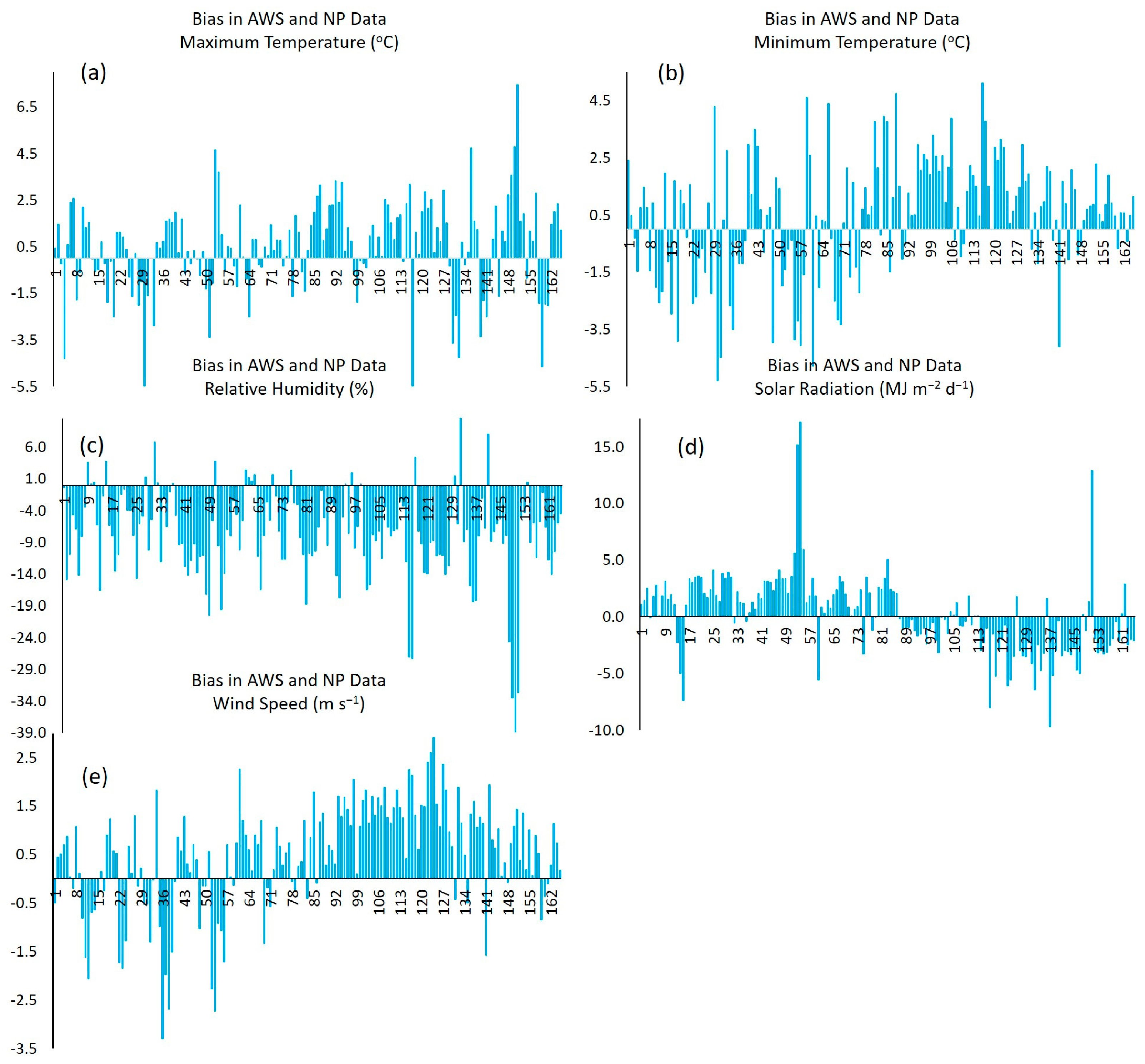
Figure 4 depicts the bias in the data recorded by the automated weather station (AWS) relative to NP platform data for the following meteorological variables: temperature (maximum and minimum), relative humidity, solar radiation, and wind speed. It is observed that 44% of the maximum temperature data evaluated (n = 165) were virtually unbiased, while 39% of NP data overestimated Tmax by 2.1 °C to 7.5 °C, and the rest of the data (17%) underestimated Tmax by 1.2 °C to 5.5 °C (Figure 4a). Regarding the minimum temperature, 39% of the data evaluated showed bias values close to zero, while 46% of the NP data overestimated Tmin by 1.6 °C to 5.1 °C and the rest (15%) underestimated Tmin by 1.8 °C to 5.3 °C (Figure 4b).

The less biased RH values (values close to zero) were observed in 16% of the evaluated data; the NP platform underestimated RH by 3.0% to 38.8% in 76% of the data, and the rest of the data (7%) overestimated RH by 5.9% to 14.9% (Figure 4c). On the other hand, 45% of the evaluated data showed the minimum differences in solar radiation bias (values between 0 MJ m⁻² d⁻¹ and 1.5 MJ m⁻² d⁻¹), while 36% of the data overestimated radiation by 3.7 MJ m⁻² d⁻¹ to 17.2 MJ m⁻² d⁻¹, and the rest of the data (19%) underestimated radiation by 2.9 MJ m⁻² d⁻¹ to 9.7 MJ m⁻² d⁻¹ (Figure 4d).

Finally, 50% of the WS data showed bias values close to zero. It is also observed that most data (41%) overestimated WS by 1.4 m s⁻¹ to 2.9 m s⁻¹, and the rest of the data (9%) underestimated WS by 1.2 m s⁻¹ to 3.3 m s⁻¹ (Figure 4e).

Based on the above, the NP platform tends to overestimate Tmax, Tmin, SR, and WS while it underestimates RH. This same behavior was reported by Jiménez et al., in the study area for Tmin, WS, and RH [27].

Estimating the 5-day cumulative ET₀ improved the values of R², r, and c relative to daily ET₀ and 5-day mean ET₀. This behavior is consistent with the one reported by Jiménez et al. [27], who obtained better R² and RMSE values when estimating 10-day mean ET₀ versus daily data. Also, this way of estimating ET₀ yielded reliability coefficients (c) rated as “very good” for BC and PM_NP and “good” for HS. However, PM_NP showed the best R², r, and c values, while HS yielded the best RMSE, PE, MBE, and b (

Table 6. Comparison and inferential parameters to determine the ET₀ equation that best fits the study area.

Parameter	Methods
	HS	BC	PM_NP	HS	BC	PM_NP	HS	BC	PM_NP
	Daily ET0 (n = 165)			5-Day Mean ET0 (n = 33)			5-Day Cumulative ET0 (n = 33)
$R^2$ (Dimensionless)	0.29	0.43	0.53	0.44	0.47	0.73	0.69	0.76	0.84
$RMSE$ (mm d−1)	1.1	1.3	1.2	0.7	1.1	0.9	3.8	5.8	4.6
$PE$ (%)	5.5	15.6	10.6	5.2	15.3	10.6	5.5	15.6	10.6
$MBE$ (mm d−1)	−0.35	−0.97	0.66	−0.32	−0.95	0.66	−1.73	−4.86	3.30
$d$ (Dimensionless)	0.94	0.99	0.98	0.85	1.00	0.94	0.86	1.00	0.94
$r$ (Dimensionless)	0.54	0.65	0.73	0.66	0.69	0.85	0.83	0.87	0.91
$c$ (Dimensionless)	0.51	0.65	0.72	0.56	0.66	0.81	0.71	0.83	0.86
$b$ (Dimensionless)	0.9270	0.8257	1.0994	0.9416	0.8399	1.1073	0.9362	0.8349	1.1075

). The latter parameter returned values close to 1, indicating that the estimated values are statistically similar to observed or reference values [16]. Some authors reported similar RMSE values (1.1 mm d⁻¹) when comparing ET₀ estimated by the HS equation and the PM method on a daily basis [71,76]. However, some authors recorded an RMSE (0.7 mm d⁻¹) for 10-day mean data, which is similar to the RMSE value obtained in the present study for 5-day cumulative ET₀ [27].

When graphically comparing the empirical equations versus the reference method (PM), daily ET₀ and 5-day mean ET₀ show a greater variability (Figure 5a,b); the 5-day cumulative ET₀ returned the best fit, with a lower variability of ET₀ values between the empirical equations and the PM method (Figure 5c).

In addition, HS yielded a better fit than the reference method (PM) in the three ways of estimating ET₀. Other authors have also reported a better fit with the HS equation relative to other methods and have taken PM as a reference for arid and semi-arid regions [16,35,76]. This equation underestimates ET₀ over most of the study period because the methods based on solar temperature and radiation do not include wind speed [19].

3.2. Comparison of Estimated ET₀ with Observed (AWS) versus Estimated (NP) Data

Table 7. Comparison and linear regression coefficients between ET₀ calculated with the reference method (FAO-56 Penman–Monteith) and HS and BC methods with temperature data from the NP platform.

Parameter	Methods
	HS_NP	BC_NP	HS_NP	BC_NP	HS_NP	BC_NP
	Daily ET0 (n = 165)		5-Day Mean ET0 (n = 33)		5-Day Cumulative ET0 (n = 33)
$R^2$ (Dimensionless)	0.29	0.38	0.55	0.45	0.75	0.74
$RMSE$ (mm d−1)	1.1	1.3	0.6	1.1	3.3	5.7
$PE$ (%)	4.4	15.0	4.1	14.6	4.4	15.0
$MBE$ (mm d−1)	−0.28	−0.93	−0.26	−0.91	−1.38	−4.67
$r$ (Dimensionless)	0.54	0.61	0.74	0.67	0.87	0.86
$a$ (Dimensionless)	2.435	−0.359	1.623	0.732	2.647	−1.700
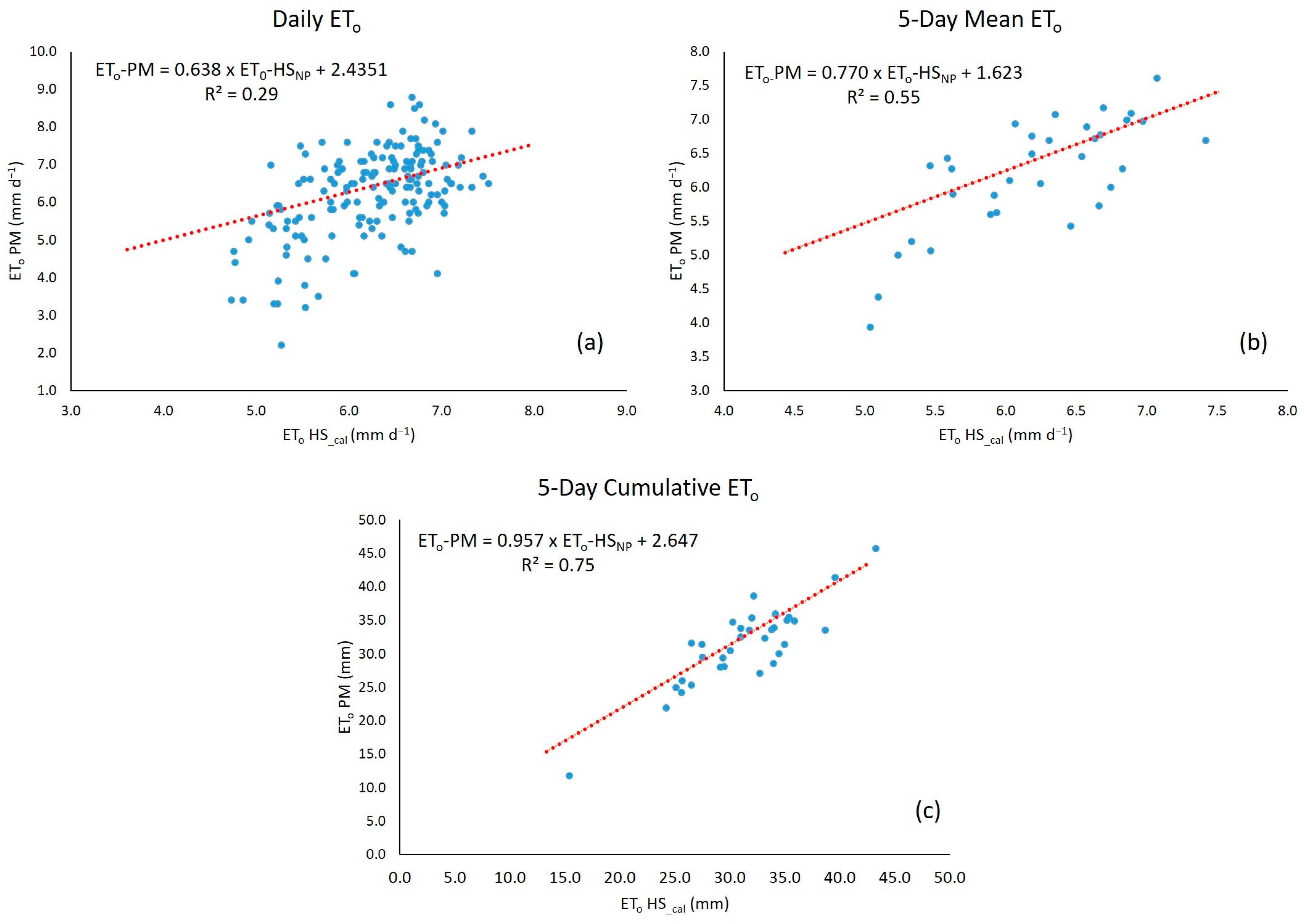
$b$ (Dimensionless)	0.638	1.244	0.770	1.033	0.957	1.240

shows the results of the goodness-of-fit tests between ET₀ calculated by the PM, HS, and BC methods, using maximum and minimum temperature data from the NP platform for the different calculation periods (daily, 5-day mean, and 5-day cumulative). The analyses of variance, with a 95% confidence interval (p-value < 0.0001), indicate a significant linear relationship between the PM method and the HS_{_NP} and BC_{_NP} equations for the three calculation periods. HS_{_NP} yielded the best values of inferential parameters versus BC_{_NP}, except for R² and r, in the daily ET₀ estimate. This indicates that HS with NP temperature data is a suitable option for estimating ET₀ for different periods. In addition, we found that the estimation percent error (PE) is lower than 5% with HS_{_NP} for the three ET₀ calculation periods. In addition, MBE is negative in the three periods, pointing to an underestimation with the HS_{_NP} method. Some authors report this same ET₀ underestimation effect in semi-arid regions during the winter–summer period [27,71].

The 5-day mean ET₀ estimate recorded the best values in most statistical parameters relative to the mean daily ET₀. However, the 5-day cumulative ET₀ estimate recorded the best r and R² values compared with the other two estimates (daily ET₀ and 5-day mean ET₀). These good results are obtained because grouping ET₀ over five days mitigates the variation in daily temperature associated with precipitation, wind speed, and cloudiness [77].

Figure 6 shows the dispersion of the calibrated HS method (HS_{_cal}) relative to PM for the different ET₀ calculation periods, depicting the best data fit obtained using data accumulated over five days.

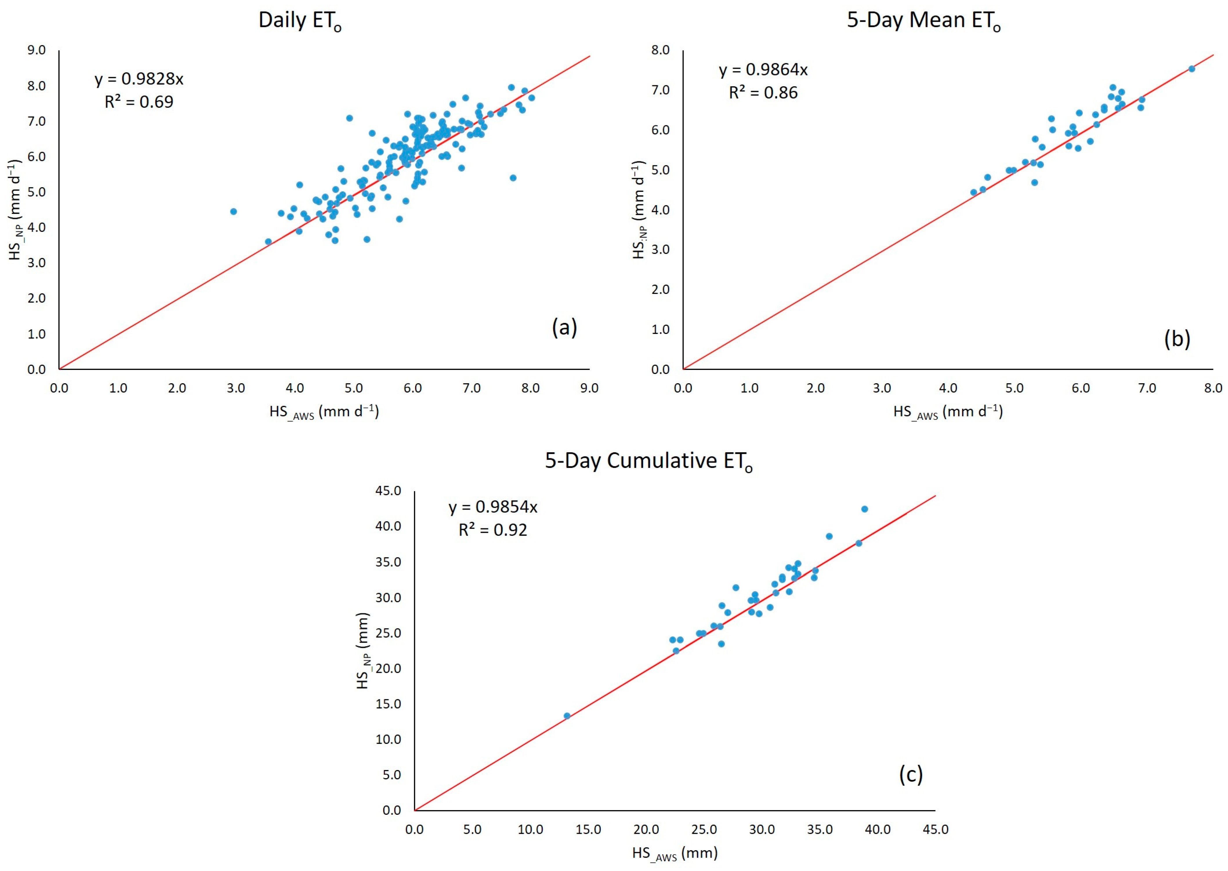
The comparison of ET₀ estimates with the HS equation using temperature data recorded by the AWS (HS_AWS) and from the NP platform (HS_NP) yielded a high correlation for the three estimates (Figure 7); the 5-day cumulative ET₀ recorded the highest R². These R² values indicate the feasibility of estimating ET₀ using the NP platform’s temperature data and the HS formula [27,71,76].

The accuracy of ET₀ calculated with methods BC and HS was compared versus the FAO-56 Penman–Monteith (PM) reference method using data from an automated weather station (AWS) and the NASA-POWER platform (NP). In this comparison, the HS equation returned the best fit in the different ways of estimating ET₀: daily, 5-day mean, and 5-day cumulative, with the latter yielding the best fit.

4. Conclusions

The Hargreaves–Samani (HS) method underestimated by 5.5% the reference evapotranspiration (ET₀) compared to the FAO-56 Penman–Monteith (PM) method considering the total ET₀ of the study period (26 February to 9 August 2021). This was because the calculation of ET₀ with the HS equation does not consider wind speed, which influences the evapotranspiration rate sometimes during the year in the study area. Nonetheless, this method is an alternative for calculating ET₀ in semi-arid regions for which only temperature records are available.

The HS equation yielded the best estimate relative to the reference method (PM) in the different ways of estimating ET₀ during the spring–summer crop cycle; the 5-day cumulative ET₀ showed the best fit. Therefore, this method is suitable for use with remote-sensing data to determine crop evapotranspiration (ET_c) with 5-day temporal resolution images. It is necessary to conduct testing of HS in various agroclimatic conditions and perform a regional spatial evaluation using data from additional automated weather stations, such as those located within the entire 017 irrigation district.

The maximum and minimum temperature data from the NASA–POWER (NP) platform was suitable for estimating ET₀ with the HS equation. This data source is a timely alternative, particularly in semi-arid regions without data from weather stations.

The results showed that NP is a reliable data source for programming medium- and low-frequency irrigation (sprinkler and surface irrigation), which are common in the study area. In addition, they provide spatially comprehensive data, unlike the point values recorded by weather stations, which could be an enormous advantage when studying large regions, such as irrigation districts.

References

- Irmak, S. Evapotranspiration. In Encyclopedia of Ecology; Academic Press: Cambridge, MA, USA, 2008; pp. 1432–1438. [Google Scholar] [CrossRef]
- Stanhill, G. Evapotranspiration. In Reference Module in Earth Systems and Environmental Sciences; Elsevier: Amsterdam, The Netherlands, 2019. [Google Scholar] [CrossRef]
- Singh, P.; Srivastava, P.K.; Mall, R.K. Estimation of potential evapotranspiration using INSAT-3D satellite data over an agriculture area. Agric. Water Manag. 2021, 2021, 143–155. [Google Scholar] [CrossRef]
- Melesse, A.M.; Weng, Q.; Thenkabail, P.S.; Senay, G.B. Remote Sensing Sensors and Applications in Environmental Resources Mapping and Modelling. Sensors 2007, 7, 3209–3241. [Google Scholar] [CrossRef] [Green Version]
- Chaudhary, S.K.; Srivastava, P.K. Future challenges in agricultural water management. Agric. Water Manag. 2021, 2021, 445–456. [Google Scholar] [CrossRef]
- Huntington, T.G. Climate Warming-Induced Intensification of the Hydrologic Cycle. Adv. Agron. 2010, 109, 1–53. [Google Scholar] [CrossRef]
- Wang, L.; Iddio, E.; Ewers, B. Introductory overview: Evapotranspiration (ET) models for controlled environment agriculture (CEA). Comput. Electron. Agric. 2021, 190, 106447. [Google Scholar] [CrossRef]
- Althoff, D.; Rodrigues, L.N. Improvement of reference crop evapotranspiration estimates using limited data for the Brazilian Cerrado. Sci. Agric. 2023, 80, 1–11. [Google Scholar] [CrossRef]
- Allen, R.G.; Pereira, L.; Raes, D.; Smith, M. Crop Evapotranspiration: Guidelines for Computing Crop Requirements; Irrigation and Drainage paper No. 56; FAO: Rome, Italy, 1998; Available online: https://www.fao.org/3/x0490e/x0490e00.htm (accessed on 1 March 2022).
- Gong, L.; Xu, C.; Chen, D.; Halldin, S.; Chen, Y.D. Sensitivity of the Penman-Monteith reference evapotranspiration to key climatic variables in the Changjiang (Yangtze River) basin. J. Hydrol. 2006, 329, 620–629. [Google Scholar] [CrossRef]
- Pereira, L.S.; Alves, I.; Paredes, P. Crop and landscape water requirements. In Reference Module in Earth Systems and Environmental Sciences; Elsevier: Amsterdam, The Netherlands, 2022. [Google Scholar] [CrossRef]
- Peng, L.; Li, Y.; Feng, H. The best alternative for estimating reference crop evapotranspiration in different sub-regions of mainland China. Sci. Rep. 2017, 7, 5458. [Google Scholar] [CrossRef] [Green Version]
- Talebmorad, H.; Ahmadnejad, A.; Eslamian, S.; Askari, K.O.A.; Singh, V.P. Evaluation of uncertainty in evapotranspiration values by FAO56-Penman-Monteith and Hargreaves-Samani methods. Int. J. Hydrol. Sci. Technol. 2020, 10, 135–147. [Google Scholar] [CrossRef]
- Wen, C.; Shuanghe, S.H.; Chunfeng, D. Sensitivity of the Penman-Monteith Reference Evapotranspiration in Growing Season in the Northwest China. In Proceedings of the International Conference on Multimedia Technology, Ningbo, China, 29–31 October 2010. [Google Scholar] [CrossRef]
- Muhammad, M.K.I.; Shahid, S.; Ismail, T.; Harun, S.; Kisi, O.; Yaseen, Z.M. The development of evolutionary computing model for simulating reference evapotranspiration over Peninsular Malaysia. Theor. Appl. Clim. 2021, 144, 1419–1434. [Google Scholar] [CrossRef]
- Raziei, T.; Pereira, L.S. Estimation of ETo with Hargreaves–Samani and FAO-PM temperature methods for a wide range of climates in Iran. Agric. Water Manag. 2013, 121, 1–18. [Google Scholar] [CrossRef]
- Gabr, M.E.-S. Management of irrigation requirements using FAO-CROPWAT 8.0 model: A case study of Egypt. Model. Earth Syst. Environ. 2022, 8, 3127–3142. [Google Scholar] [CrossRef]
- Surendran, U.; Sushanth, C.M.; Joseph, E.J.; Al-Ansari, N.; Yasseen, Z.M. FAO CROPWAT Model-Based Irrigation Requirements for Coconut to Improve Crop and Water Productivity in Kerala, India. Sustainability 2019, 11, 5132. [Google Scholar] [CrossRef] [Green Version]
- Ortiz, R.S.; Chile, A.M. Métodos de cálculo para estimar la evapotranspiración de referencia para el Valle de Tumbaco. Siembra 2020, 7, 70–79. [Google Scholar] [CrossRef]
- Yamaç, S.S. Reference Evapotranspiration Estimation With kNN and ANN Models Using Different Climate Input Combinations in the Semi-arid Environment. J. Agric. Sci. Tarim Bilimleri Dergisi 2021, 27, 129–137. [Google Scholar] [CrossRef]
- Sahoo, B.; Walling, I.; Deka, B.C.; Bhatt, B.P. Standardization of Reference Evapotranspiration Models for a Subhumid Valley Rangeland in the Eastern Himalayas. J. Irrigat. Drain. Eng. 2012, 138, 880–895. [Google Scholar] [CrossRef]
- Srivastava, A.; Sahoo, B.; Raghuwanshi, N.S.; Singh, R. Evaluation of Variable-Infiltration Capacity Model and MODIS-Terra Satellite-Derived Grid-Scale Evapotranspiration Estimates in a River Basin with Tropical Monsoon-Type Climatology. J. Irrig. Drain. Eng. 2017, 143, 04017028. [Google Scholar] [CrossRef] [Green Version]
- Allen, R.G.; Pereira, L.S.; Raes, D.; Smith, M. Evapotranspiración del cultivo: Guías para la determinación de los requerimientos de agua de los cultivos. In FAO Riego y Drenaje Manual 56; FAO: Rome, Italy, 2006; Available online: https://www.fao.org/3/x0490s/x0490s00.htm (accessed on 15 May 2022).
- Gavilán, M.P.; Estévez, J.; Berengena, J. ETo estandarizada en el sur de España ¿Cuál debe ser la referencia? In Proceedings of the XXXIV Congreso Nacional de Riegos, Escuela Universitaria de Ingeniería Técnica Agrícola, Sevilla, Spain, 7–9 June 2016; Available online: https://idus.us.es/bitstream/handle/11441/41070/T-A-01.pdf?sequence=1&isAllowed=y (accessed on 23 July 2023).
- Borges, J.C.F.; Anjos, R.J.; Silva, T.J.A.; Lima, J.R.S.; Andrade, C.L.T. Métodos de estimativa da evapotranspiração de referência diária para a microrregião de Garanhuns, PE. Rev. Bras. Eng. Agrí Amb. 2012, 16, 380–390. [Google Scholar] [CrossRef] [Green Version]
- Woldesenbet, T.A.; Elagib, N.A. Spatial-temporal evaluation of different reference evapotranspiration methods based on the climate forecast system reanalysis data. Hydrol. Process. 2021, 36, e14239. [Google Scholar] [CrossRef]
- Jiménez, J.S.I.; Ojeda, B.W.; Inzunza, I.M.A.; Marcial, P.M.D.J. Analysis of the NASA-POWER system for estimating reference evapotranspiration in the Comarca Lagunera, Mexico. Ing. Agrícola Biosist. 2021, 13, 201–226. [Google Scholar] [CrossRef]
- Luo, Y.; Chang, X.; Peng, S.; Khan, S.; Wang, W.; Zheng, Q.; Cai, X. Short-term forecasting of daily reference evapotranspiration using the Hargreaves-Samani model and temperature forecasts. Agric. Water Manag. 2014, 136, 42–51. [Google Scholar] [CrossRef]
- Perera, K.C.; Western, A.W.; Nawarathna, B.; George, B. Forecasting daily reference evapotranspiration for Australia using numerical weather prediction outputs. Agric. For. Meteorol. 2014, 194, 50–63. [Google Scholar] [CrossRef]
- Xiong, Y.; Luo, Y.; Wang, Y.; Traore, S.; Xu, J.; Jiao, X.; Fipps, G. Forecasting daily reference evapotranspiration using the Blaney-Criddle model and temperature forecasts. Arch. Agron. Soil. Sci. 2015, 62, 790–805. [Google Scholar] [CrossRef]
- Goh, E.H.; Ng, J.L.; Huang, Y.F.; Yong, S.L.S. Performance of potential evapotranspiration models in Peninsular Malaysia. J. Water Clim. Chang. 2021, 12, 3170–3186. [Google Scholar] [CrossRef]
- Fooladmand, H.R. Evaluation of some equations for estimating evapotranspiration in the south of Iran. Arch. Agron. Soil. Sci. 2011, 57, 741–752. [Google Scholar] [CrossRef]
- Hafeez, M.; Ahmad, C.Z.; Akhtar, K.A.; Bakhsh, G.A.; Basit, A.; Tahira, F. Comparative Analysis of Reference Evapotranspiration by Hargreaves and Blaney-Criddle Equations in Semi-Arid Climatic Conditions. Curr. Res. Agric. Sci. 2020, 7, 52–57. [Google Scholar] [CrossRef]
- Martinez, C.J.; Thepadia, M. Estimating Reference Evapotranspiration with Minimum Data in Florida. J. Irrig. Drain. Eng. 2010, 136, 494–501. [Google Scholar] [CrossRef]
- Tabari, H. Evaluation of Reference Crop Evapotranspiration Equations in Various Climates. Water Resour. Manag. 2010, 24, 2311–2337. [Google Scholar] [CrossRef]
- Lima, J.R.d.S.; Antonino, A.C.D.; Souza, E.S.d.; Hammecker, C.; Montenegro, S.M.G.L.; Lira, C.A.B.d.O. Calibration of Hargreaves-Samani Equation for Estimating Reference Evapotranspiration in Sub-Humid Region of Brazil. J. Water Resour. Prot. 2013, 5, 1–5. [Google Scholar] [CrossRef] [Green Version]
- Temesgen, B.; Eching, S.; Davidoff, B.; Frame, K. Comparison of Some Reference Evapotranspiration Equations for California. J. Irrig. Drain. Eng. 2005, 131, 73–84. [Google Scholar] [CrossRef]
- Todorovic, M.; Karic, B.; Pereira, L.S. Reference evapotranspiration estimate with limited weather data across a range of Mediterranean climates. J. Hydrol. 2013, 481, 166–176. [Google Scholar] [CrossRef] [Green Version]
- Shahidian, S.; Serralheiro, R.P.; Serrano, J.; Teixeira, J.L. Parametric calibration of the Hargreaves-Samani equation for use at new locations. Hydrol. Process. 2012, 27, 605–616. [Google Scholar] [CrossRef]
- Sepaskhah, A.R.; Razzaghi, F. Evaluation of the adjusted Thornthwaite and Hargreaves-Samani methods for estimation of daily evapotranspiration in a semi-arid region of Iran. Arch. Agron. Soil. Sci. 2009, 55, 51–66. [Google Scholar] [CrossRef]
- Hafeez, M.; Chatha, Z.A.; Bakhsh, A.; Basit, A.; Khan, A.A.; Tahira, F. Reference Evapotranspiration by Hargreaves and Modified Hargreaves Equations under Semi-Arid Environment. Curr. Res. Agric. Sci. 2020, 7, 58–63. [Google Scholar] [CrossRef]
- Martins, D.S.; Paredes, P.; Raziei, T.; Pires, C.; Cadima, J.; Pereira, L.S. Assessing reference evapotranspiration estimation from reanalysis weather products. An application to the Iberian Peninsula. Int. J. Climatol. 2016, 37, 2378–2397. [Google Scholar] [CrossRef]
- Paredes, P.; Martins, D.S.; Pereira, L.S.; Cadima, J.; Pires, C. Accuracy of daily estimation of grass reference evapotranspiration using ERA-Interim reanalysis products with assessment of alternative bias correction schemes. Agric. Water Manag. 2018, 210, 340–353. [Google Scholar] [CrossRef]
- Pelosi, A.; Terribile, F.; D’Urso, G.; Chirico, G. Comparison of ERA5-Land and UERRA MESCAN-SURFEX Reanalysis Data with Spatially Interpolated Weather Observations for the Regional Assessment of Reference Evapotranspiration. Water 2020, 12, 1669. [Google Scholar] [CrossRef]
- Rodrigues, G.C.; Braga, R.P. Evaluation of NASA POWER Reanalysis Products to Estimate Daily Weather Variables in a Hot Summer Mediterranean Climate. Agronomy 2021, 11, 1207. [Google Scholar] [CrossRef]
- Park, J.; Choi, M. Estimation of evapotranspiration from ground-based meteorological data and global land data assimilation system (GLDAS). Stoch. Environ. Res. Risk Assess. 2015, 29, 1963–1992. [Google Scholar] [CrossRef]
- Tian, D.; Martinez, C.J.; Graham, W.D. Seasonal Prediction of Regional Reference Evapotranspiration Based on Climate Forecast System Version 2. J. Hydrometeorol. 2014, 15, 1166–1188. [Google Scholar] [CrossRef]
- Peters, L.C.D.; Kumar, S.V.; Mocko, D.M.; Tian, Y. Estimating evapotranspiration with land data assimilation systems. Hydrol. Process. 2011, 25, 3979–3992. [Google Scholar] [CrossRef] [Green Version]
- McEvoy, D.J.; Roj, S.; Dunkerly, C.; McGraw, D.; Huntington, J.L.; Hobbins, M.T.; Ott, T. Validation and Bias Correction of Forecast Reference Evapotranspiration for Agricultural Applications in Nevada. J. Water Resour. Plan. Manag. 2022, 148, 04022057. [Google Scholar] [CrossRef]
- Blankenau, P.A.; Kilic, A.; Allen, R. An evaluation of gridded weather data sets for the purpose of estimating reference evapotranspiration in the United States. Agric. Water Manag. 2020, 242, 106376. [Google Scholar] [CrossRef]
- Ndiaye, P.M.; Bodian, A.; Diop, L.; Deme, A.; Dezetter, A.; Djaman, K.; Ogilvie, A. Trend and Sensitivity Analysis of Reference Evapotranspiration in the Senegal River Basin Using NASA Meteorological Data. Water 2020, 12, 1957. [Google Scholar] [CrossRef]
- Negm, A.; Jabro, J.; Provenzano, G. Assessing the suitability of American National Aeronautics and Space Administration (NASA) agro-climatology archive to predict daily meteorological variables and reference evapotranspiration in Sicily, Italy. Agric. For. Meteorol. 2017, 244–245, 111–121. [Google Scholar] [CrossRef]
- Srivastava, P.K.; Singh, P.; Mall, R.K.; Pradhan, R.K.; Bray, M.; Gupta, A. Performance assessment of evapotranspiration estimated from different data sources over agricultural landscape in Northern India. Theor. Appl. Clim. 2020, 140, 145–156. [Google Scholar] [CrossRef]
- Rodrigues, G.C.; Braga, R.P. Estimation of Daily Reference Evapotranspiration from NASA POWER Reanalysis Products in a Hot Summer Mediterranean Climate. Agronomy 2021, 11, 2077. [Google Scholar] [CrossRef]
- Davis. Instrumentos Climáticos de Precisión. Catálogo Global. 2020. Available online: https://cdn.shopify.com/s/files/1/0515/5992/3873/files/Weather_Catalog_Spanish.pdf (accessed on 10 February 2020).
- Instituto Nacional de Estadística y Geografía (INEGI). Continuo de Elevaciones Mexicano (CEM 3.0), Coahuila. 2013. Available online: https://www.inegi.org.mx/app/geo2/elevacionesmex/ (accessed on 19 July 2023).
- Instituto Nacional de Estadística y Geografía (INEGI). Uso de Suelo y Vegetación, Conjunto de Datos Vectoriales de Uso del Suelo y Vegetación. Escala 1:250 000. Serie VII. 2018. Available online: https://www.inegi.org.mx/temas/usosuelo/ (accessed on 21 July 2023).
- White, J.W.; Hoogenboom, G.; Stackhouse, P.W.; Hoell, J.M. Evaluation of NASA satellite- and assimilation model-derived long-term daily temperature data over the continental US. Agric. For. Meteorol. 2008, 148, 1574–1584. [Google Scholar] [CrossRef] [Green Version]
- Zhang, T.; Chandler, W.S.; Hoell, J.M.; Westberg, D.; Whitlock, C.H.; Stackhouse, P.W. A Global Perspective on Renewable Energy Resources: Nasa’s Prediction of Worldwide Energy Resources (Power) Project. In Proceedings of the ISES World Congress 2007, Beijing, China, 18–21 September 2007; Springer: Berlin/Heidelberg, Germany, 2007; Volumes 1–5, pp. 2636–2640. [Google Scholar] [CrossRef]
- Monteiro, L.A.; Sentelhas, P.C.; Pedra, G.U. Assessment of NASA/POWER satellite-based weather system for Brazilian conditions and its impact on sugarcane yield simulation. Int. J. Climatol. 2017, 38, 1571–1581. [Google Scholar] [CrossRef]
- Zhang, T.; Stackhouse, P.W.; Gupta, S.K.; Cox, S.J.; Mikovitz, J.C. Validation and Analysis of the Release 3.0 of the NASA GEWEX Surface Radiation Budget Dataset. AIP Conf. Proc. 2009, 1100, 597–600. [Google Scholar] [CrossRef]
- National Aeronautics and Space Administration. Prediction of Worldwide Energy Resource. 2023. Available online: https://power.larc.nasa.gov/ (accessed on 18 March 2023).
- Allen, R.G.; Pruitt, W.O.; Businger, J.A.; Fritschen, L.J.; Jensen, M.E.; Quinn, F.H. Capítulo 4 Evaporation and Transpiration. In ASCE Handbook of Hydrology; American Society of Civil Engineers: Reston, VA, USA, 1996; pp. 125–252. [Google Scholar] [CrossRef]
- Hargreaves, G.H.; Samani, Z.A. Reference crop evapotranspiration from ambient air temperature. Appl. Eng. Agric. 1985, 1, 96–99. [Google Scholar] [CrossRef]
- Chávez, R.E.; González, C.G.; González, B.J.L.; Dzul, L.E.; Sánchez, C.I.; López, S.A.; Chávez, S.J.A. Uso de estaciones climatológicas automáticas y modelos matemáticos para determinar la evapotranspiración. Tecnol. Cienc. Agua 2013, 4, 115–126. Available online: https://www.scielo.org.mx/pdf/tca/v4n4/v4n4a7.pdf (accessed on 23 June 2022).
- Doorenbos, J.; Pruitt, W.O. Guidelines for Predicting Crop Water Requirements; Irrigation and Drainage Paper FAO-24; FAO: Rome, Italy, 1977; Available online: https://www.fao.org/publications/card/en/c/6bae3071-5d7b-5206-af5c-c9bfa1d9d1fe/ (accessed on 29 May 2022).
- Silva, G.H.d.; Dias, S.H.B.; Ferreira, L.B.; Santos, J.É.O.; Cunha, F.F.d. Performance of different methods for reference evapotranspiration estimation in Jaíba, Brazil. Rev. Bras. Eng. Agríc. Amb. 2018, 22, 83–89. [Google Scholar] [CrossRef] [Green Version]
- Debnath, S.; Adamala, S.; Raghuwanshi, N.S. Sensitivity Analysis of FAO-56 Penman-Monteith Method for Different Agro-ecological Regions of India. Environ. Process. 2015, 2, 689–704. [Google Scholar] [CrossRef]
- Jerszurki, D.; de Souza, J.L.M.; Ramos, S.L.d.C. Sensitivity of ASCE-Penman-Monteith reference evapotranspiration under different climate types in Brazil. Clim. Dyn. 2019, 53, 943–956. [Google Scholar] [CrossRef]
- Ndiaye, P.M.; Bodian, A.; Diop, L.; Djaman, K. Sensitivity Analysis of the Penman-Monteith Reference Evapotranspiration to Climatic Variables: Case of Burkina Faso. J. Water Resour. Prot. 2017, 9, 1364–1376. [Google Scholar] [CrossRef] [Green Version]
- Villa, C.A.O.; Ontiveros, C.R.E.; Ruíz, A.O.; González, S.A.; Quevedo, T.J.A.; Ordoñez, H.L.M. Spatio-temporal variation of reference evapotranspiration from empirical methods in Chihuahua, Mexico. Ing. Agrícola Biosist. 2021, 13, 95–115. [Google Scholar] [CrossRef]
- Maldonado, W.; Valeriano, T.T.B.; de Souza, R.G. EVAPO: A smartphone application to estimate potential evapotranspiration using cloud gridded meteorological data from NASA-POWER system. Comput. Electron. Agric. 2019, 156, 187–192. [Google Scholar] [CrossRef]
- Duarte, Y.C.N.; Sentelhas, P.C. NASA/POWER and DailyGridded weather datasets—How good they are for estimating maize yields in Brazil? Int. J. Biometeorol. 2020, 64, 319–329. [Google Scholar] [CrossRef]
- Quansah, A.D.; Dogbey, F.; Asilevi, P.J.; Boakye, P.; Darkwah, L.; Oduro, K.S.; Sokama, N.Y.A.; Mensah, P. Assessment of solar radiation resource from the NASA-POWER reanalysis products for tropical climates in Ghana towards clean energy application. Sci. Rep. 2022, 12, 10684. [Google Scholar] [CrossRef]
- De Pondeca, M.S.F.V.; Manikin, G.S.; DiMego, G.; Benjamin, S.G.; Parrish, D.F.; Purser, R.J.; Wan, S.W.; Horel, J.D.; Myrick, D.T.; Lin, Y.; et al. The Real-Time Mesoscale Analysis at NOAA’s National Centers for Environmental Prediction: Current Status and Development. Weather Forecast. 2011, 26, 593–612. [Google Scholar] [CrossRef]
- Najmaddin, P.M.; Whelan, M.J.; Balzter, H. Estimating Daily Reference Evapotranspiration in a Semi-Arid Region Using Remote Sensing Data. Remote Sens. 2017, 9, 779. [Google Scholar] [CrossRef] [Green Version]
- Texeira, P.; Pannunzio, A.; Brenner, J. Calibración de la ecuación de Hargreaves para el cálculo de la evapotranspiración de cultivo de referencia (ETo) en Salto, Uruguay. Rev. Climatol. 2021, 21, 80–88. Available online: https://rclimatol.eu/wp-content/uploads/2021/06/Articulo21g.pdf (accessed on 23 June 2023).
Figure 1.
Location of the automated weather station (AWS).
Figure 2.
Altitude map of Module XII.
Figure 3.
Reference evapotranspiration estimated with the FA0-56 Penman–Monteith method using AWS meteorological data (blue points) and rainfall recorded in the study period (red bars).
Figure 4.
Bias between observed (AWS) and reference (NP) data for the meteorological. (a) Bias in AWS and NP Data Tmax. (b) Bias in AWS and NP Data Tmin. (c) Bias in AWS and NP Data RH. (d) Bias in AWS and NP Data SR. (e) Bias in AWS and NP Data WS.
Figure 5.
Different ways to estimate ET0 using empirical equations and the reference method (PM) during the study period. (a) Estimation Daily ET0. (b) Estimation 5-Day Mean ET0. (c) Estimation 5-Day Cumulative ET0.
Figure 6.
Dispersion plot of the calibrated HS method (HS_NP) relative to the FAO-56 Penman–Monteith (PM) reference method for the different ET0 calculation periods: Daily (a), 5-Day Mean (b) 5-Day Cumulative (c).
Figure 7.
Linear relationship between ET0 estimates with the HS equation using temperature data from the AWS and the NP platform for the different ET0 calculation periods: Daily (a), 5-Day Mean (b) 5-Day Cumulative (c).