


Robust Fusion Kalman Estimator of the Multi-Sensor Descriptor System with Multiple Types of Noises and Packet Loss
School of Mathematics, Physics and Statistics, Shanghai University of Engineering Science, Shanghai 201620, China
*
Author to whom correspondence should be addressed.
Sensors 2023, 23(15), 6968; https://doi.org/10.3390/s23156968
Submission received: 22 March 2023
/
Revised: 26 May 2023
/
Accepted: 3 August 2023
/
Published: 5 August 2023
(This article belongs to the Section Intelligent Sensors)
Abstract
:Under the influence of multiple types of noises, missing measurement, one-step measurement delay and packet loss, the robust Kalman estimation problem is studied for the multi-sensor descriptor system (MSDS) in this paper. Moreover, the established MSDS model describes uncertain-variance noises, multiplicative noises, time delay and packet loss phenomena. Different types of noises and packet loss make it more difficult to build the estimators of MSDS. Firstly, MSDS is transformed to the new system model by applying the singular value decomposition (SVD) method, augmented state and fictitious noise approach. Furthermore, the robust Kalman estimator is constructed for the newly deduced augmented system based on the min-max robust estimation principle and Kalman filter theory. In addition, the given estimator consists of four parts, which are the usual Kalman filter, predictor, smoother and white noise deconvolution estimator. Then, the robust fusion Kalman estimator is obtained for MSDS according to the relation of augmented state and the original system state. Simultaneously, the robustness is demonstrated for the actual Kalman estimator of MSDS by using the mathematical induction method and Lyapunov’s equation. Furthermore, the error variance of the obtained Kalman estimator is guaranteed to the upper bound for all admissible uncertain noise variance. Finally, the simulation example of a circuit system is examined to illustrate the performance and effectiveness of the robust estimators.
1. Introduction
The descriptor system is also a singular system, which has a broader structure than the normal system. Furthermore, the descriptor system can describe the non-causal phenomena in real systems, such as robot systems, power systems, image modeling, and economic systems [1,2,3]. The state estimation problem of the descriptor system has been a popular topic in recent years. Many research results and methods have been obtained to solve the estimation problem [4,5,6,7,8,9,10,11,12]. Based on the reduced-order Kalman estimation algorithm [13,14], the singular value decomposition (SVD) method for the descriptor system is presented in [4,7]. The authors of [5] give the least squares method and the maximum likelihood method for the descriptor systems, respectively. In [8], the time domain Wiener filter for the descriptor system is proposed by using the modern time series analysis method. However, the above estimation problems are only studied for the known general descriptor systems.
Moreover, it is well known that the estimator based on the classical Kalman filtering requires that noise statistics and the model parameters are exactly known [11]. However, in many practical systems, there exist many uncertainties such as modelling errors, unmodeled dynamic, random perturbations, missing measurements, measurement delays, multiplicative noises and so on [15,16,17,18]. In order to solve the effect of the uncertainty, the robust estimation is studied for an uncertain system [11]. At present, for the uncertain descriptor system, the Kalman robust filter and predictor are presented [12]. The robust time-varying estimator is proposed for descriptor systems with random one-step measurement delay by using the SVD method, the augmented method, and the fictitious noise approach [19]. However, it should be noted that reference [19] only considers the descriptor with a one-step measurement delay, and other uncertainties are not considered. In [20], the robust centralized and weighted observation fusion (CAWOF) prediction algorithm is derived for the uncertain MSDS with multiplicative noise by using the SVD method and the minimax robustness estimation criterion. Reference [20] only considers the descriptor system with multiplicative noise and uncertain noise. However, packet loss and measurement delay problems have not been taken into account. In [21], the uncertain-variance noises and packet loss problems are solved in the MSDS; however, the effects of multiplicative noise and measurement delay are not considered in the MSDS.
In addition, the estimation accuracy and performance of a single sensor descriptor system can be easily affected by the stability and reliability of the sensor [22]. To improve estimation accuracy and guarantee performance of the considered system, a multi-sensor system has been widely used [23]. For the multi-sensor descriptor system, Kalman filtering is a fundamental tool due to its recursive structure and excellent performance. In general, the fusion method of the Kalman filter can be categorized into three types: centralized fusion, measurement fusion, and distributed state fusion method [24,25]. In [24,26], the authors present distributed fusion algorithms that use optimally weighted fusion criteria with a matrix weight, a diagonal matrix weight, and a scalar weight. These algorithms the address estimation problems in multi-sensor systems, which are typically studied based on the known parameters of the system model and the complete known noise statistical structure. In [25], the fusion Kalman filter algorithm deals with an uncertain nonsingular system with multiplicative noises, missing measurements, and linearly correlated white noises with uncertain variances. However, for a multi-sensor networked descriptor control system, the distributed fusion robust Kalman filter algorithm is proposed in [27]. However, reference [27] only considers uncertain-variance correlated noises and missing measurement problems of the multi-sensor networked descriptor control system.
To date, the robust fusion estimation problem is not solved for MSDS with uncertain-variance noises, multiplicative noises and a unified measurement model, which totally include five kinds of uncertainties which are uncertain-variance noises, multiplicative noises, missing measurements, one-step measurement delays and packet dropouts. Motivated by the aforementioned analysis, for MSDS with the above five uncertainties, the robust estimation problem will be studied. The main contributions and innovations of this paper are as follows: (1) The considered MSDS is novel and challenging, which includes uncertain-variance noises, multiplicative noises, missing measurements, one-step measurement delays and packet dropouts. (2) Applying the SVD method, the augmented state method and the fictitious white noises method, MSDS is transformed to a new standard system only with uncertain-variance noise. (3) Based on the Kalman filter and the relations of the original MSDS and the newly obtained system, the robust Kalman estimators are given for MSDS and the newly obtained augmented system. (4) The robustness is proved for the proposed estimators by using the Lyapunov equation approach and the mathematical induction method.
This paper is organized into seven sections. In Section 2, the system model is given. In Section 3, a new standard augmented state model is presented. The robust Kalman estimator for descriptor system is discussed in Section 4. In Section 5, a robust analysis is discussed. Section 6 presents the numerical simulation results. Finally, Section 7 provides the conclusion.
2. System Description and Preliminaries
Consider MSDS with uncertain-variance noises, multiplicative noises and a unified measurement model
where t is a discrete time, is the state, is the input, is additive process noise, is additive measurement noise, is the ith noise-free measurement, is multiplicative state-dependent noise, is the measurement of the ith sensor, is the measurement received by estimator to be designed, and L are the number of multiplicative noises and sensors, respectively. M, , , B and are constant matrices with suitable dimensions.
Assumption 1.
M is a singular matrix, , , that is, det , and the system (1) is regular.
Assumption 2.
, and are mutually independent random sequences, obeying Bernoulli distributions with known probabilities of taking 1 or 0, such that
from Assumption 2, it follow that
zero-means white noises , and are defined as follows:
it follow that
Assumption 3.
, and are mutually independent white noises with zero means and the unknown actual variance are , and , respectively, and
The unknown actual variance are, respectively, have known conservative upper bounds, which are
Remark 1.
In real-world measurement, time delay and packet loss may occur at any time. The measurement models (2)–(4) describe a unified measurement model by introducing random sequences , and , which include the missing measurements, one-step delay measurement and packet dropouts. If , , then . If , , then , which means measurement missed. If , , then , which means that there is one-step measurement delay. If , , then , which means packet dropout.
3. New Standard Augmented State Model with Uncertain-Variance Fictitious Noises
Applying the SVD approach, there are non-singular matrices P and Q satisfying
letting
substituting (15) and (16) into (1) yields
then we have two new subsystems
where , , , , , , in (16) and (17) are substituted into (2), then it is easy to obtain
substituting (20) into yields
substituting (21) into (3), it is easy to obtain
from (9), we have , in (22), replacing by yields
where × , substituting (23) into (4), replacing by and replacing by yield
where . In order to facilitate the calculation, it is necessary to simplify . New parameters and are defined, then we can rewrite as
where , defining new white noise variances as follows
let
then it is easy to obtain the new standard augmented state apace model as follows
where
Non-central second order moments are defined as , and , they satisfy the following Lyapunov equations
and we have corresponding upper values
with initial values , , .
For the new process noise in (28), it has corresponding conservative variance and real variance . Similarly, for new measurement noise in (29), it has corresponding conservative variance and real variance .
Let , is actual variance of , the conservative and actual noise variances and are given as follows
Let , then is the actual variance of , the conservative and actual noise variances and are given as follows
Substituting (25) into in (27), we have
where , , we can obtain the conservative and actual variances and as follows
where , . Defining and , we have
where , then we have
the conservative and actual cross-covariance and are defined as follows
Lemma 1
([28]). (i) Let , then . (ii) Let , and , , then . (iii) Let , then for arbitrary , .
Parameters , , , and are defined as , , , , .
Theorem 1.
For all admissible uncertain variance , , in (13), all of the following inequalities are true, that is,
Proof of Theorem 1.
From (31) and (32), it is easy to obtain
with the initial condition , , applying Lemma 1, iterating (44) yield .
Rewriting as follows
where .
Let , , , from (35), we have
since , , and , based on Lemma 1, it is easy to obtain
applying Lemma 1, we can easily obtain , from (31), (32) and (40), it is easy to obtain as follows
then we have
we can easily obtain , with the initial condition . According to (50) and applying mathematical induction, yield , since , , from (40), yield .
4. Robust Kalman Estimator of Descriptor System
4.1. Conservative Kalman Estimator of New State Space Model
For the new standard system (28) and (29), applying the Kalman filtering algorithm [29] yields the optimal Kalman estimator (include filter , predictor , smoother )
where , and the conservative prediction error variance satisfies the Riccati equation
The one-step predicting error is defined as
where .
Furthermore, the conservative and the actual variance and are defined as follows
The conservative and actual one-step prediction error variance and can be rewritten as the following Lyapunov function
with the initial values .
Furthermore, the optimal conservative white noise deconvolution estimator of fictitious noise is
where , noise estimation error is defined as , then it is easy to obtain
where ,
The conservative and actual estimation error variances and are defined as follows
The conservative and actual estimation error variances and of are defined as follows
4.2. Conservative Kalman Estimator of Original Descriptor System
Theorem 2.
For the uncertain MSDS (1)–(4) with Assumptions 1–3, the robust Kalman estimator is obtained as follows
where
where
5. Robust Analysis
Theorem 3.
Proof of Theorem 3.
According to (59), it is easy to obtain
rewriting as follows
where
since , , we have , applying Lemma 1, we have , then .
Parameters , , and are defined as follows:
from (60) and (61) and (67), it is easy to obtain
with the initial condition , applying mathematical induction method, yield
From (72), defining , we have
substituting (78) into (80), yield
then (81) can be rewritten as
where , applying Lemma 1, we have
. Taking the trace of , we can easily obtain . The Proof of Theorem 3 is completed. □
6. Simulation
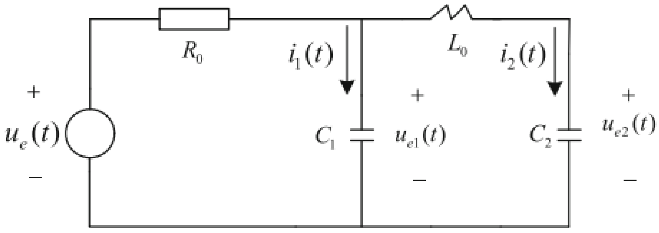
Consider the circuits system shown in Figure 1, is control input, , , and are resister, inductor and capacities, respectively. The MSDS model is given as follows
where, , and are the voltage of and , and are the current of and , is zero mean white noise, the variance is .
Taking the sample period s, the brief parameter matrices are as follows:
Let , , , , , , , , , , . Furthermore, the following matrices in (15) as given as
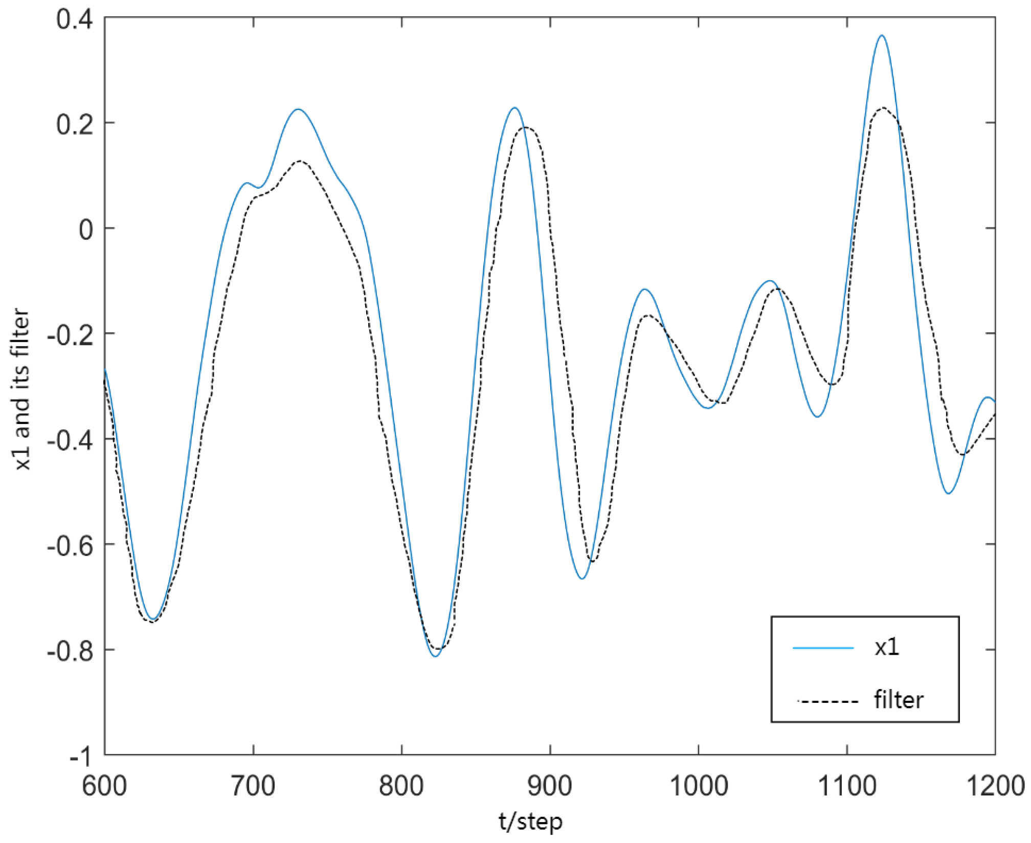
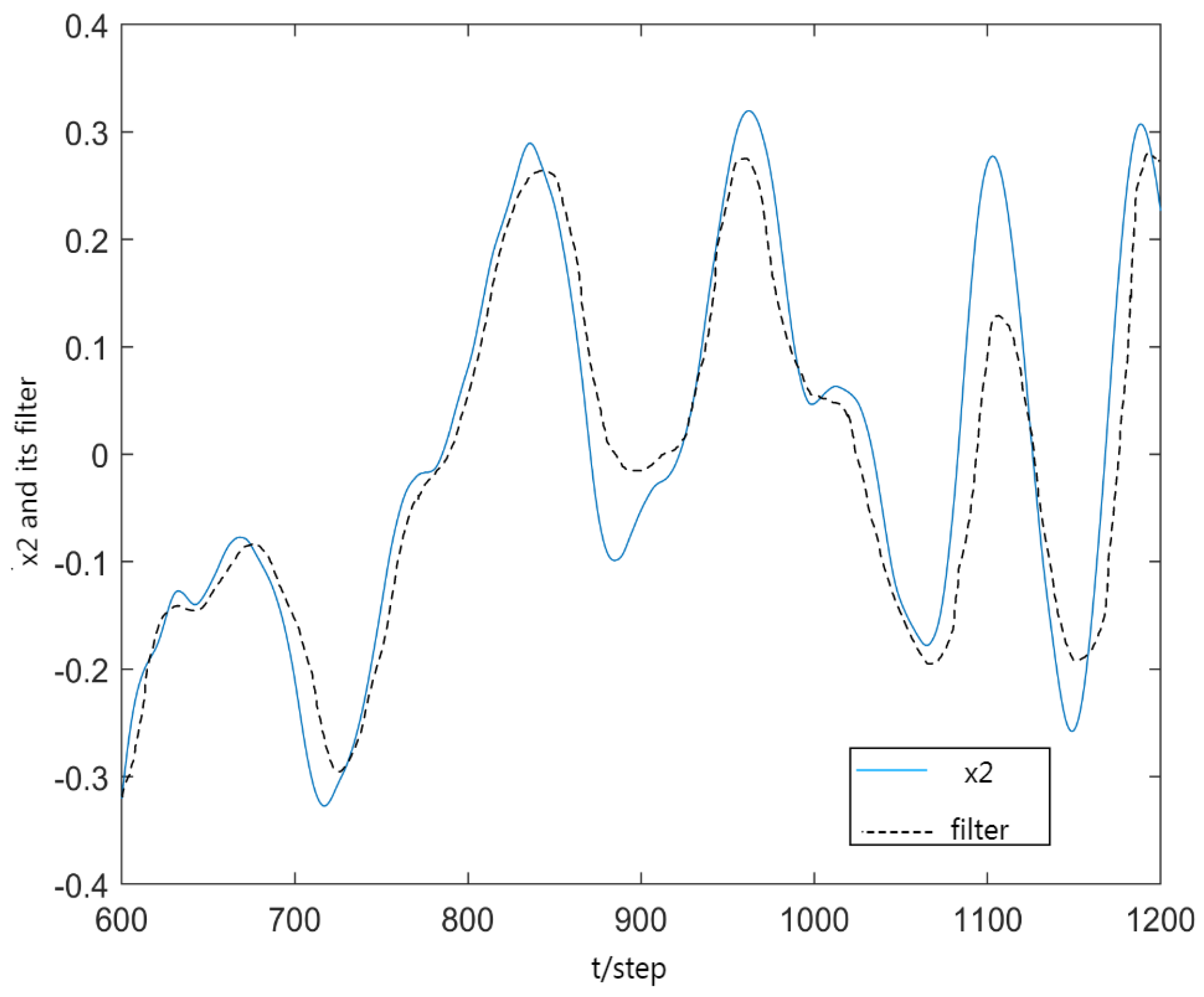
Figure 2 and Figure 3 gives the first and second components of actual state , and corresponding filters , from to , where the solid curves denote the true state components and the dotted curves denote . From Figure 3, the every component of robust filter can effectively follow the true state component .
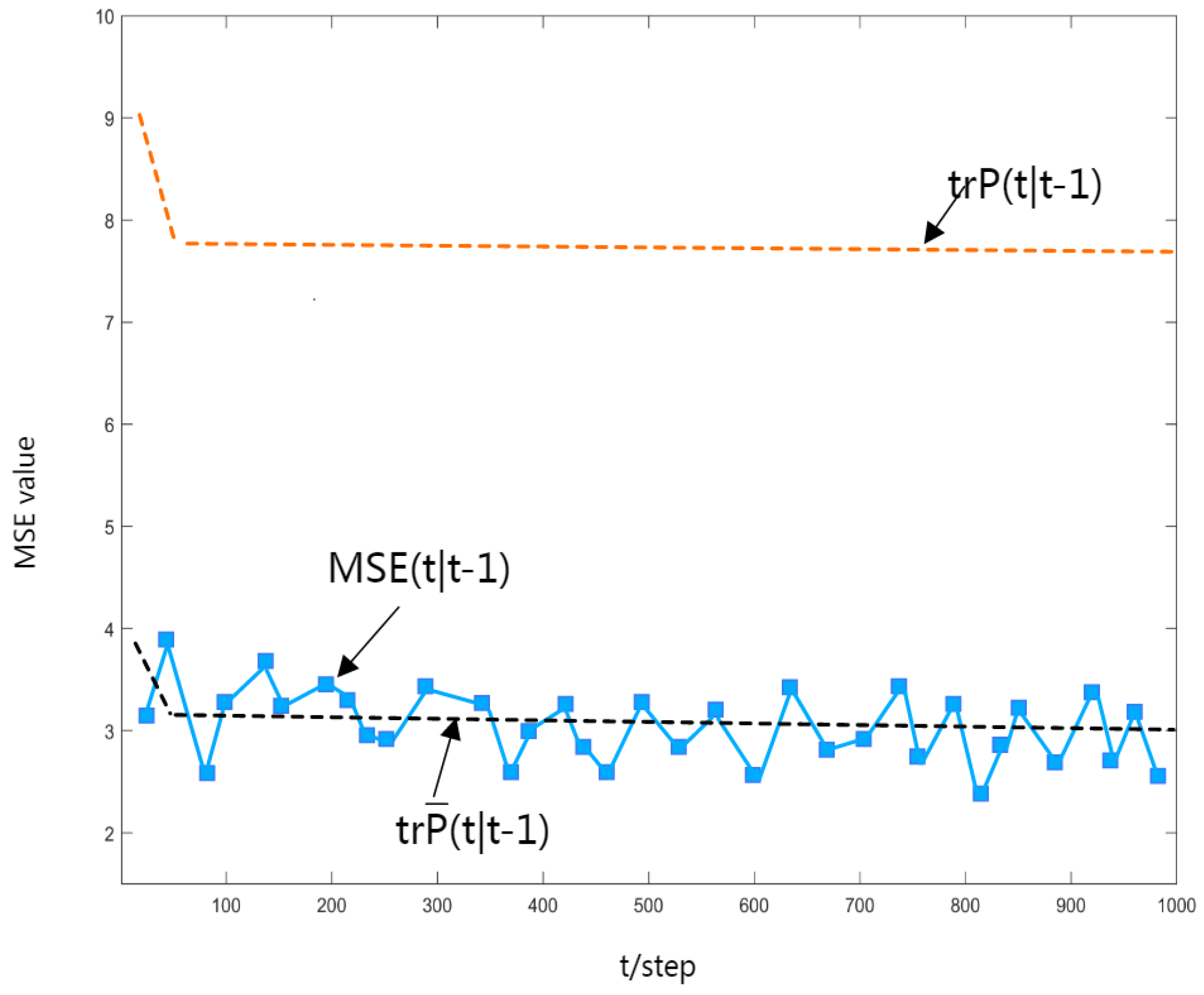
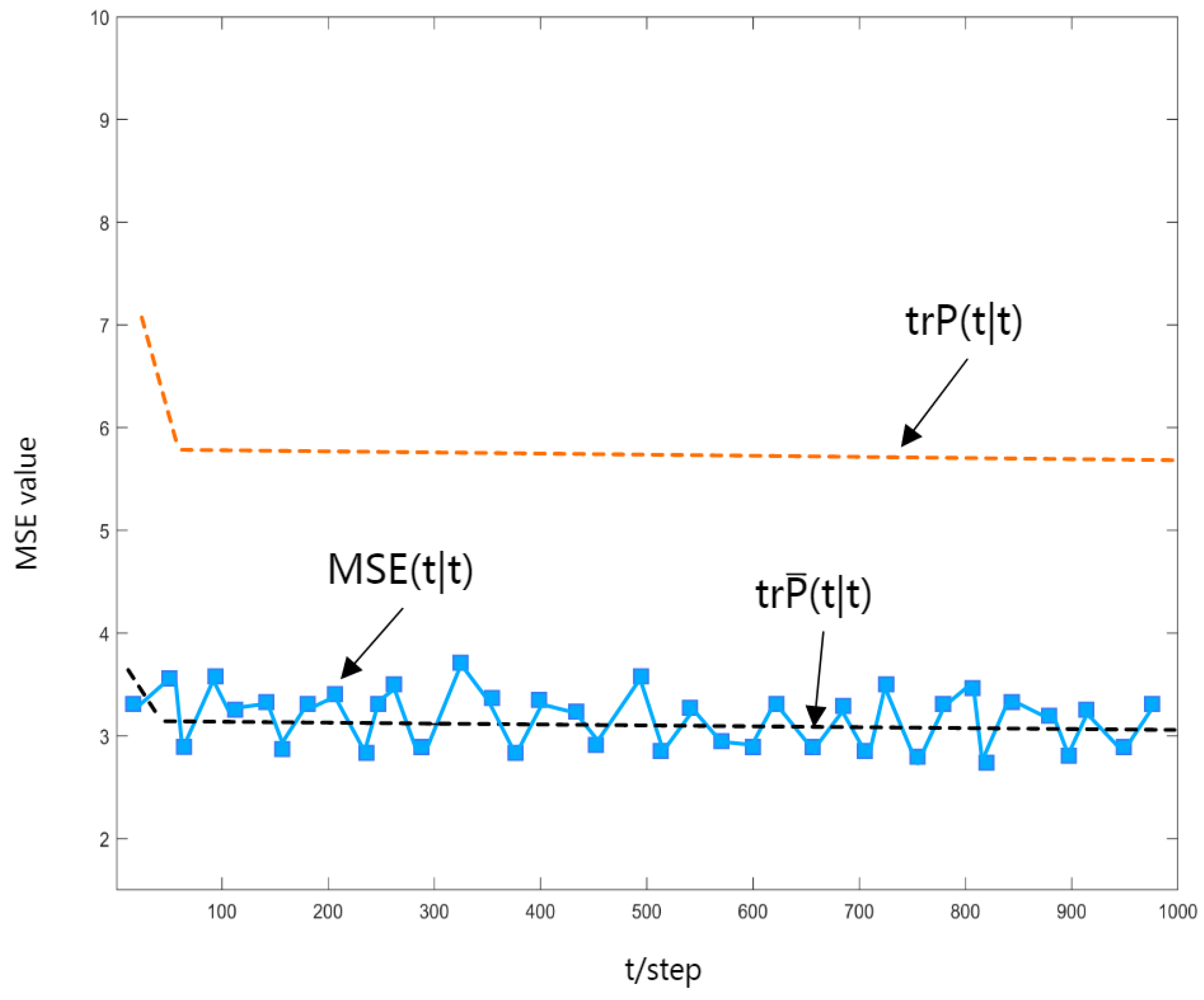
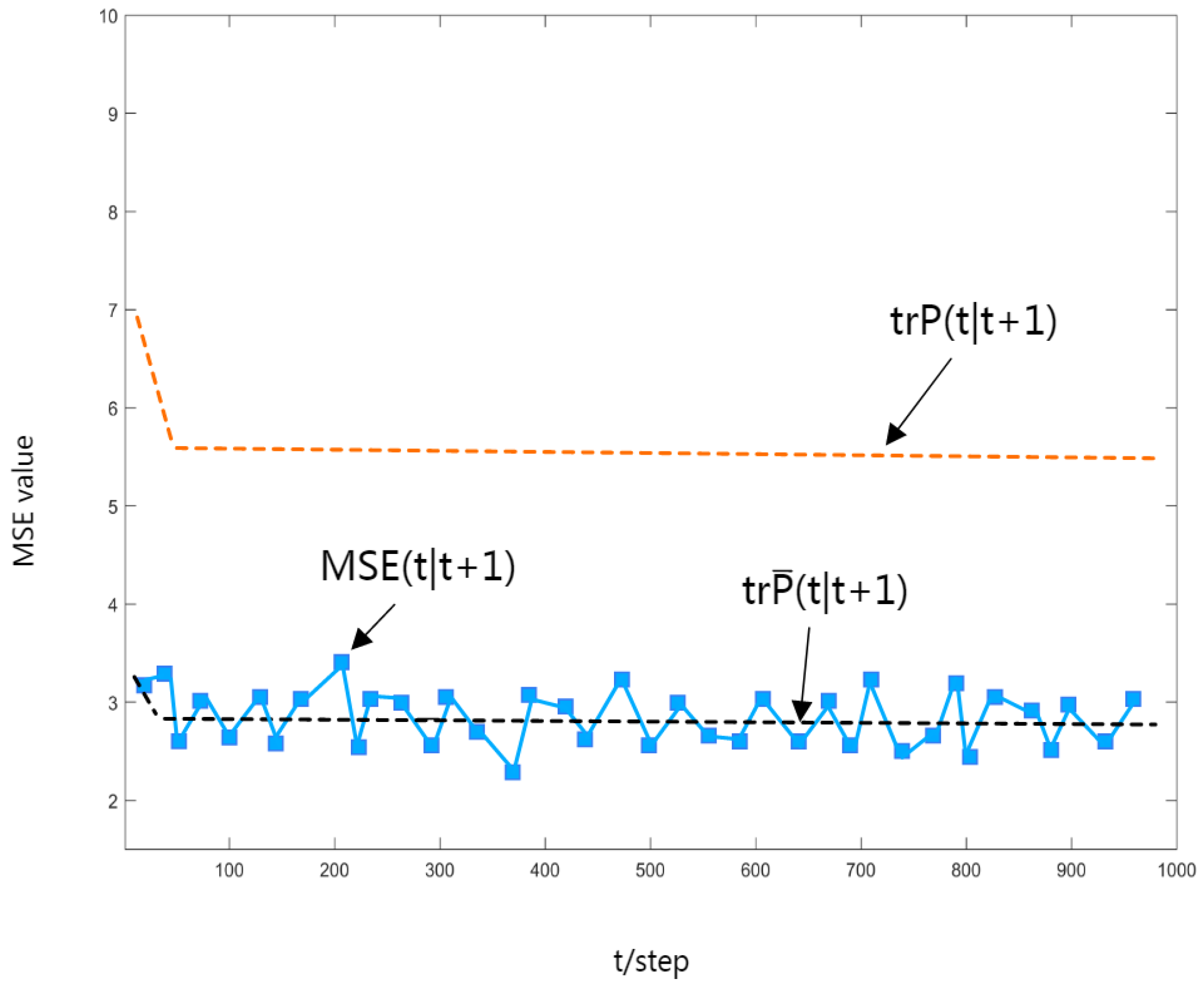
To verify the correctness of the obtained robust Kalman estimator, a Monte Carlo simulation is performed, and the mean square error (MSE) curve of the robust time-varying estimator is shown in Figure 4, Figure 5 and Figure 6. It is easy to see that the value of MSE can be approximated to the value of tr, and as Theorem 3 states, it has an upper bound tr.
In Figure 4, Figure 5 and Figure 6, the dashed black line shows the trace of the actual estimated error variance, the curved line shows the MSE value, and the dashed orange line shows the actual upper bound on the variance of the estimation error.
Remark 2.
Time delay is not considered in references [20,21,22,23,24,25,26,27]. Meanwhile, references [19,20,21] do not consider missing measurement, references [19,21,27] ignore the multiplicative noise, and references [19,20,25,27] do not consider packet dropouts. In Table 1, the model of this paper contains more influencing factors, and it is more general than references [19,20,21,22,23,24,25,26,27].
7. Conclusions
In this paper, the robust Kalman estimation of multi-sensor linear singular systems is studied. The singular value decomposition (SVD) method, the augmented state method and the fictitious noise method are applied to transform the original generalized system into a new standard system with uncertain-variance noise. Based on the minimum–maximum robust estimation principle and Kalman filtering theory, a new robust Kalman estimator for augmented systems is obtained. According to the relationship between the augmented state and the original system state, the robust Kalman estimator of the original system is given. Using mathematical induction and the Lyapunov equation method, the robustness of the actual Kalman estimator to the original system is proved. In the future, we will investigate time-varying robust Kalman estimators for a multi-sensor descriptor system with a measurement delay and packet loss. Furthermore, we will consider an uncertain multi-sensor descriptor system in which multiplicative noise occurs simultaneously in both the system and the measurement models, and study the corresponding Kalman filter.
The limitation of this paper is that it uses a general method for studying singular systems. In the future, we will explore some novel methods to study the problem of robust estimation of multi-sensor singular systems
Author Contributions
Methodology, J.Z.; Software, J.Z.; Formal analysis, W.C.; Writing—original draft, J.Z.; Writing—review & editing, S.S.; Supervision, W.C. All authors have read and agreed to the published version of the manuscript.
Funding
This research received no external funding.
Institutional Review Board Statement
Not applicable.
Informed Consent Statement
Not applicable.
Data Availability Statement
Not applicable.
Conflicts of Interest
The authors declare no conflict of interest.
References
- Luenberger, D. Dynamic equations in descriptor form. IEEE Trans. Autom. Control 1977, 22, 312–321. [Google Scholar] [CrossRef]
- Hasan, M.A.; Azim-Sadjani, M.R. Noncausal image modeling using descriptor approach. IEEE Trans. Circuits Syst. II 1995, 42, 536–540. [Google Scholar] [CrossRef] [Green Version]
- Dai, L. Singular Control Systems; Springer: Berlin, Germany, 1989. [Google Scholar]
- Deng, Z.L.; Gao, Y.; Tao, G.L. Reduced-order steady-state descriptor Kalman fuser weighted by block-diagonal matrices. Inf. Fusion 2008, 9, 300–309. [Google Scholar] [CrossRef]
- Ishihara, J.Y.; Terra, M.H.; Campos, J.C.T. Optimal recursive estimation for discrete-time descriptor systems. Int. J. Syst. Sci. 2008, 36, 605–615. [Google Scholar] [CrossRef]
- Dou, Y.F.; Sun, S.; Ran, C.J. Self-tuning full-order WMF Kalman filter for multisensor descriptor systems. IET Control. Theory. Appl. 2017, 11, 359–368. [Google Scholar] [CrossRef]
- Sun, S.L.; Ma, J. Optimal filtering and smoothing for discrete-time stochastic singular systems. Signal Process 2007, 87, 189–201. [Google Scholar] [CrossRef]
- Deng, Z.L.; Xu, Y. Descriptor Wiener state estimators. Automatica 2000, 36, 1761–1766. [Google Scholar] [CrossRef]
- Bai, Y.; Wang, X.; Jin, X. A neuron-based kalman filter with nonlinear autoregressive model. Sensors 2020, 20, 299. [Google Scholar] [CrossRef] [Green Version]
- Luttmann, L.; Mercorelli, P. Comparison of backpropagation and Kalman filter-based training for neural networks. In Proceedings of the 2021 25th International Conference on System Theory, Control and Computing (ICSTCC), Iasi, Romania, 20–23 October 2021; pp. 234–241. [Google Scholar]
- Lewis, F.L.; Xie, L.X.; Popa, D. Optimal and Robust Estimation, 2nd ed.; CRC Press: New York, NY, USA, 2008. [Google Scholar]
- Ishihara, J.Y.; Terra, M.H. Robust state prediction for descriptor systems. Automatica 2008, 44, 2185–2190. [Google Scholar] [CrossRef]
- Kalman, R.E. A new approach to linear filtering and prediction problems. J. Basic Eng. 1960, 82, 35–45. [Google Scholar] [CrossRef] [Green Version]
- Kalman, R.E.; Bucy, R.S. New Results in Linear Filtering and Prediction Theory. J. Basic Eng. 1961, 83, 95–108. [Google Scholar] [CrossRef] [Green Version]
- Wang, Z.D.; Ho, D.W.C.; Liu, X.H. Variance-constrained filtering for uncertain stochastic systems with missing measurements. IEEE Trans. Syst. Man Cybern. 2003, 48, 1254–1258. [Google Scholar]
- Sun, S.; Xie, L.; Xiao, W.; Soh, Y.C. Optimal linear estimation for systems with multiple packet dropouts. Automatica 2008, 44, 1333–1342. [Google Scholar] [CrossRef]
- Nahi, N. Optimal recursive estimation with uncertain observation. IEEE Trans. Inf. Theory 1969, 15, 457–462. [Google Scholar] [CrossRef]
- Sun, S.L.; Lin, H.L.; Ma, J.; Li, X.Y. Multi-sensor distributed fusion estimation with applications in networked systems: A review paper. Inf. Fusion 2017, 38, 122–134. [Google Scholar]
- Shen, H.; Dou, Y.; Ran, C. Robust time-varying estimator for descriptor system with random one-step measurement delay. Optim. Control Appl. Meth. 2021, 42, 1775–1793. [Google Scholar] [CrossRef]
- Tao, G.; Liu, W.; Wang, X.; Zhang, J.; Yu, H. Robust CAWOF Kalman predictors for uncertain multi-sensor generalized system. Int. J. Adapt. Control Signal Process 2021, 35, 2423–2445. [Google Scholar] [CrossRef]
- Liu, W.; Zheng, J.; Dou, Y.; Ran, C. Robust fusion filter for multisensor descriptor system with uncertain-variance noises and packet dropout. Optim. Control Appl. Meth. 2022, 43, 1401–1421. [Google Scholar] [CrossRef]
- Salahshoor, K.; Mosallaei, M.; Bayat, M. Centralized and decentralized process and sensor fault monitoring using data fusion based on adaptive extended Kalman filter algorithm. Measurement 2008, 41, 1059–1076. [Google Scholar] [CrossRef]
- Liggins, M.E.; Hall, D.L.; Llinas, J. Handbook of multisensor data fusion: Theory and practice. Artech. House Radar. Lib. 2008, 39, 180–184. [Google Scholar]
- Sun, S.L. Multi-sensor optimal information fusion Kalman filters with applications. Aerosp. Sci. Technol. 2004, 8, 57–62. [Google Scholar] [CrossRef]
- Wang, X.; Liu, W.; Deng, Z. Robust weighted fusion Kalman estimators for systems with multiplicative noises, missing measurements and uncertain-variance linearly correlated white noises. Aerosp. Sci. Technol. 2017, 68, 331–344. [Google Scholar] [CrossRef]
- Deng, Z.L.; Gao, Y.; Mao, L.; Li, Y.; Hao, G. New approach to information fusion steady-state Kalman filtering. Automatica 2005, 41, 1695–1770. [Google Scholar] [CrossRef]
- Zheng, J.; Ran, C. Distributed fusion robust estimators for multisensor networked singular control system with uncertain-variance correlated noises and missing measurement. Comput. Appl. Math. 2023, 42, 66. [Google Scholar] [CrossRef]
- Ran, C.; Deng, Z. Robust fusion Kalman estimators for networked mixed uncertain systems with random one-step measurement delays, missing measurements, multiplicative noises and uncertain noise variances. Inf. Sci. 2020, 534, 27–52. [Google Scholar] [CrossRef]
- Anderson, B.; Moore, J. Optimal Filtering; Prentice-Hall: Englewood Clifs, NJ, USA, 1979. [Google Scholar]
Figure 1.
The circuit system.

Figure 2.
and its filter .

Figure 3.
and its filter .

Figure 4.
MSE curve.

Figure 5.
MSE curve.

Figure 6.
MSE curve.


Table 1.
Model comparisons.
| Model | This Paper | [19] | [20] | [21] | [25] | [27] |
|---|---|---|---|---|---|---|
| Uncertain-variance noise | √ | √ | √ | √ | √ | √ |
| Multiplicative noise | √ | × | √ | × | √ | × |
| Missing measurement | √ | × | × | × | √ | √ |
| Time delay | √ | √ | × | × | × | × |
| Packet dropouts | √ | × | × | √ | × | × |
| Multi-sensor descriptor system | √ | × | √ | √ | × | √ |
Where “√” means that the model contains this component, and “×” means that the model does not contain this component.
Disclaimer/Publisher’s Note: The statements, opinions and data contained in all publications are solely those of the individual author(s) and contributor(s) and not of MDPI and/or the editor(s). MDPI and/or the editor(s) disclaim responsibility for any injury to people or property resulting from any ideas, methods, instructions or products referred to in the content. |
© 2023 by the authors. Licensee MDPI, Basel, Switzerland. This article is an open access article distributed under the terms and conditions of the Creative Commons Attribution (CC BY) license (https://creativecommons.org/licenses/by/4.0/).
Share and Cite
MDPI and ACS Style
Zheng, J.; Cui, W.; Sun, S. Robust Fusion Kalman Estimator of the Multi-Sensor Descriptor System with Multiple Types of Noises and Packet Loss. Sensors 2023, 23, 6968. https://doi.org/10.3390/s23156968
AMA Style
Zheng J, Cui W, Sun S. Robust Fusion Kalman Estimator of the Multi-Sensor Descriptor System with Multiple Types of Noises and Packet Loss. Sensors. 2023; 23(15):6968. https://doi.org/10.3390/s23156968
Chicago/Turabian StyleZheng, Jie, Wenxia Cui, and Sian Sun. 2023. "Robust Fusion Kalman Estimator of the Multi-Sensor Descriptor System with Multiple Types of Noises and Packet Loss" Sensors 23, no. 15: 6968. https://doi.org/10.3390/s23156968
Note that from the first issue of 2016, this journal uses article numbers instead of page numbers. See further details here.