

Explorative Data Analysis Methods: Application to Laser-Induced Breakdown Spectroscopy Field Data Measured on the Island of Vulcano, Italy
 , , , and
Abstract
:1. Introduction
2. Methods
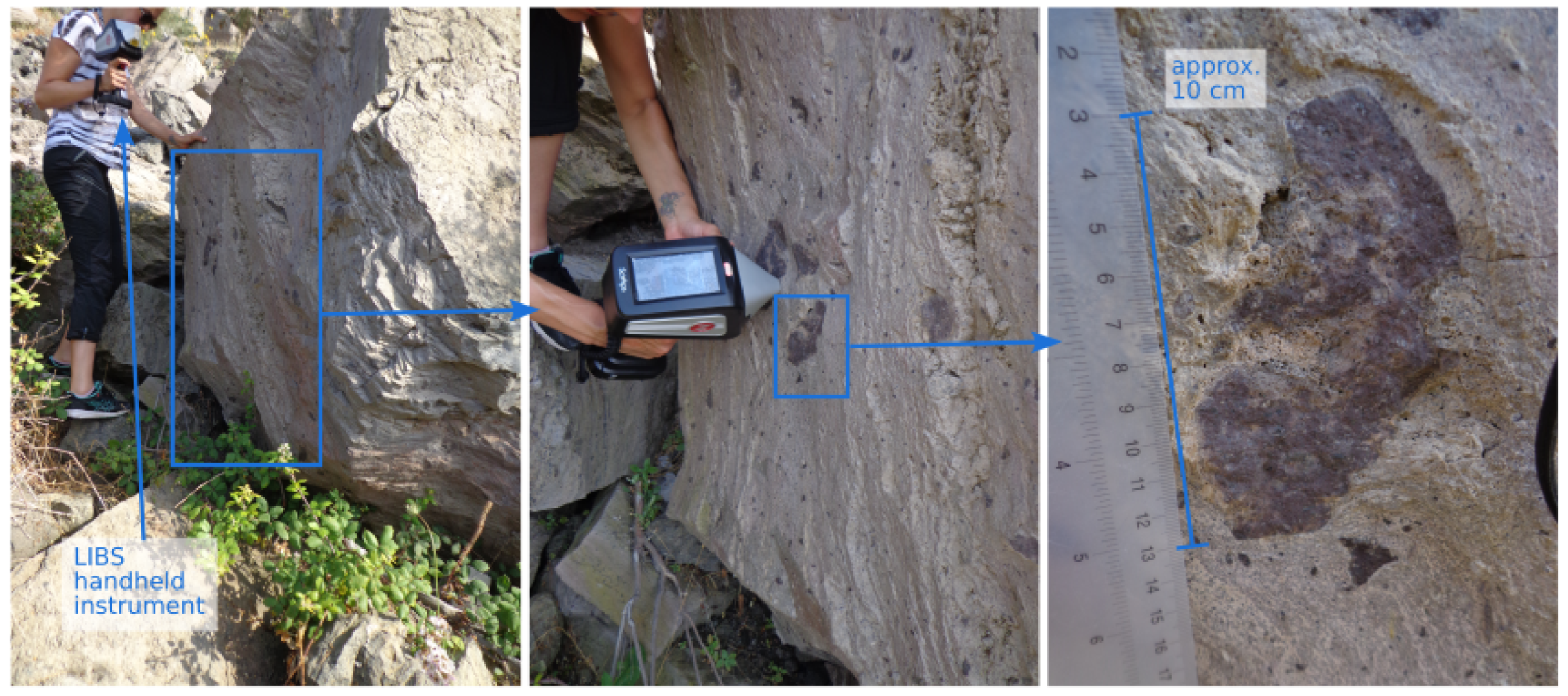
2.1. LIBS Handheld Device
2.2. Data Analysis Techniques
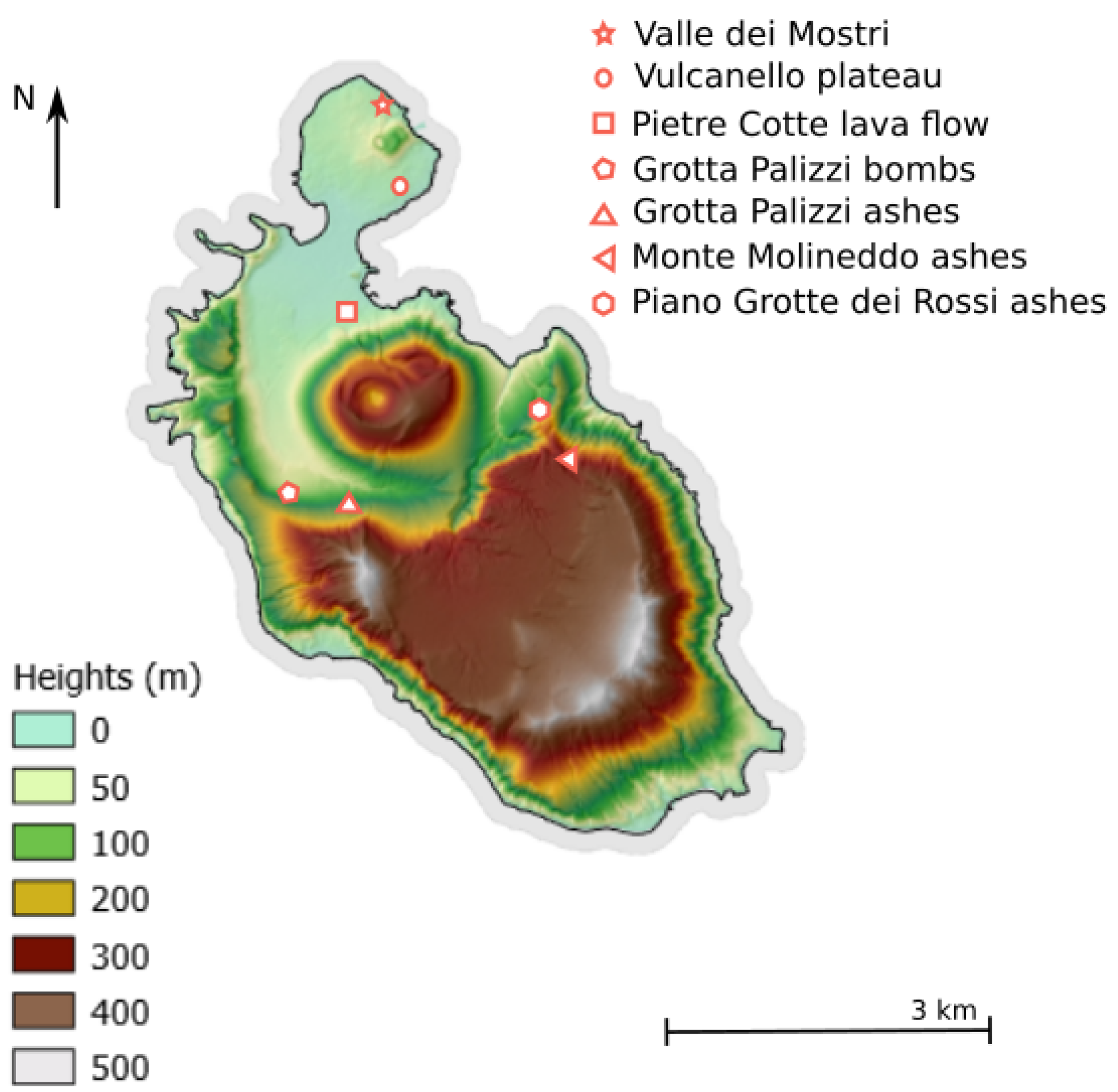
3. Measurement Location
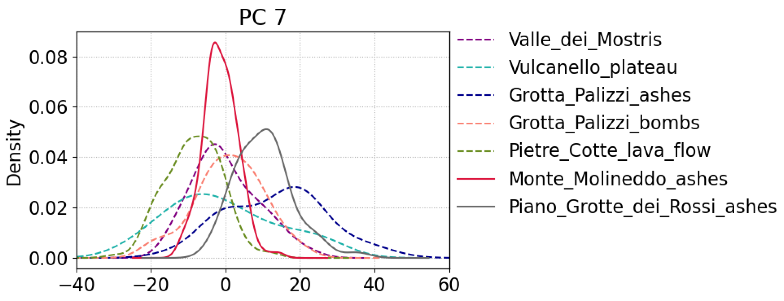
- Pietre Cotte lava flow: texturally heterogeneous and quasi-obsidianaceous lava flow, with a rhyolitic glassy groundmass that contains lati-trachytic enclaves [35].
- Grotta Palizzi: In the location known as Vallonazzo (rough valley) two different sets of measurements were conducted on products from the Grotta Palizzi formation (GP2a in [32]). The former set of analyses was performed on consolidated ashes organized in thinly-bedded/cross-stratified fashion labeled as Grotta Palizzi ashes. At the top of this formation, also pumiceous lapilli and bread-crust bombs are present and are here characterized in the second set of analyses named Grotta Palizzi bombs.
- Monte Molineddo ashes: This is a consolidated, thinly-bedded vari-colored ashes outcrop belonging to the Monte Molineddo Formation (ml in [32])
- Piano Grotte dei Rossi ashes: Although located close to the Monte Molineddo ashes this outcrop is different in geomorphology as it consists of dark, planar to cross-bedded ashes belonging to the Piano Grotte dei Rossi Formation (gr in [32]).
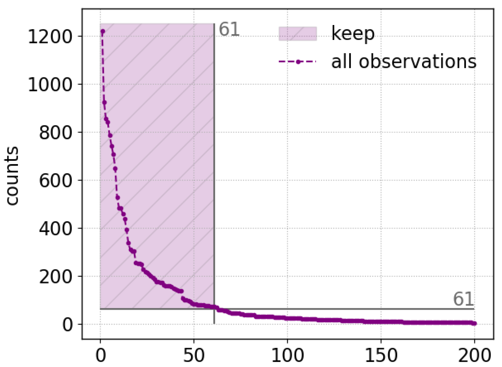
4. Dataset and Data Processing
5. Results
5.1. PCA Results
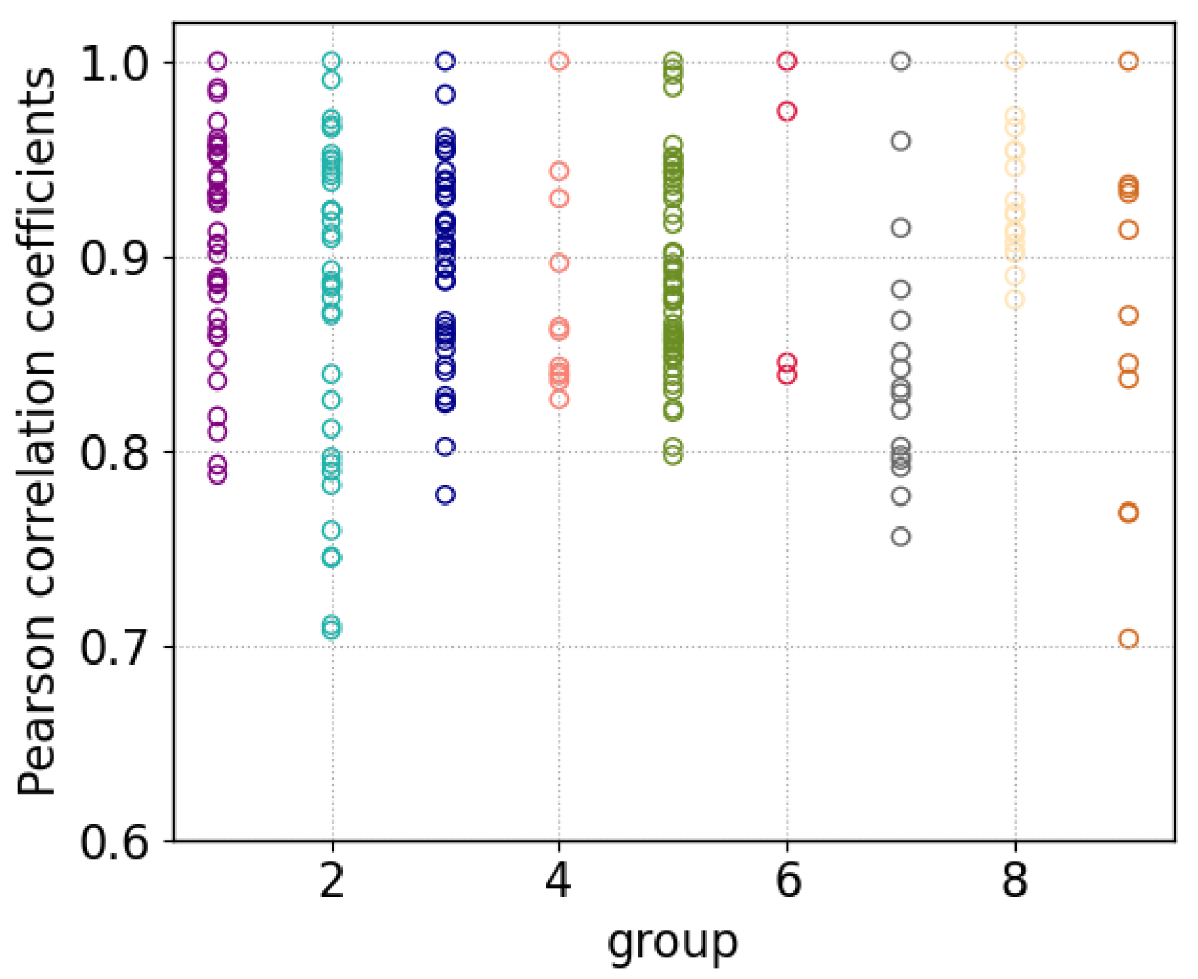
5.2. IFF Results
5.3. Combined Results
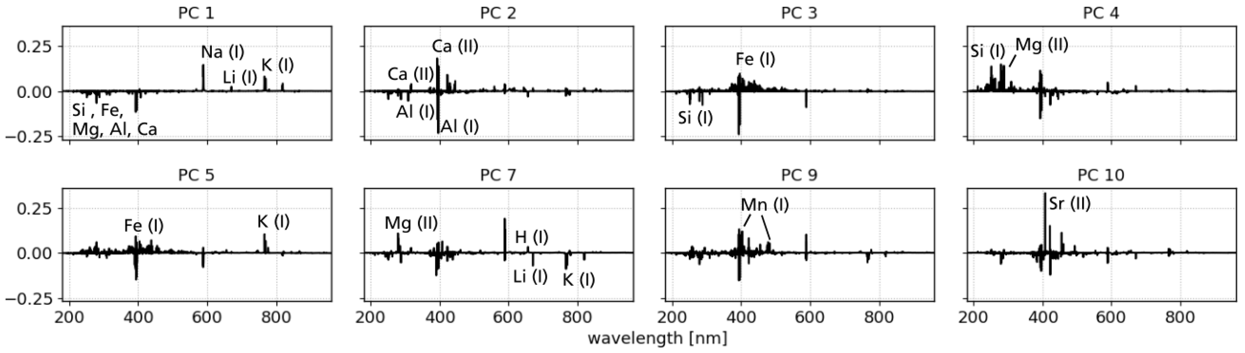
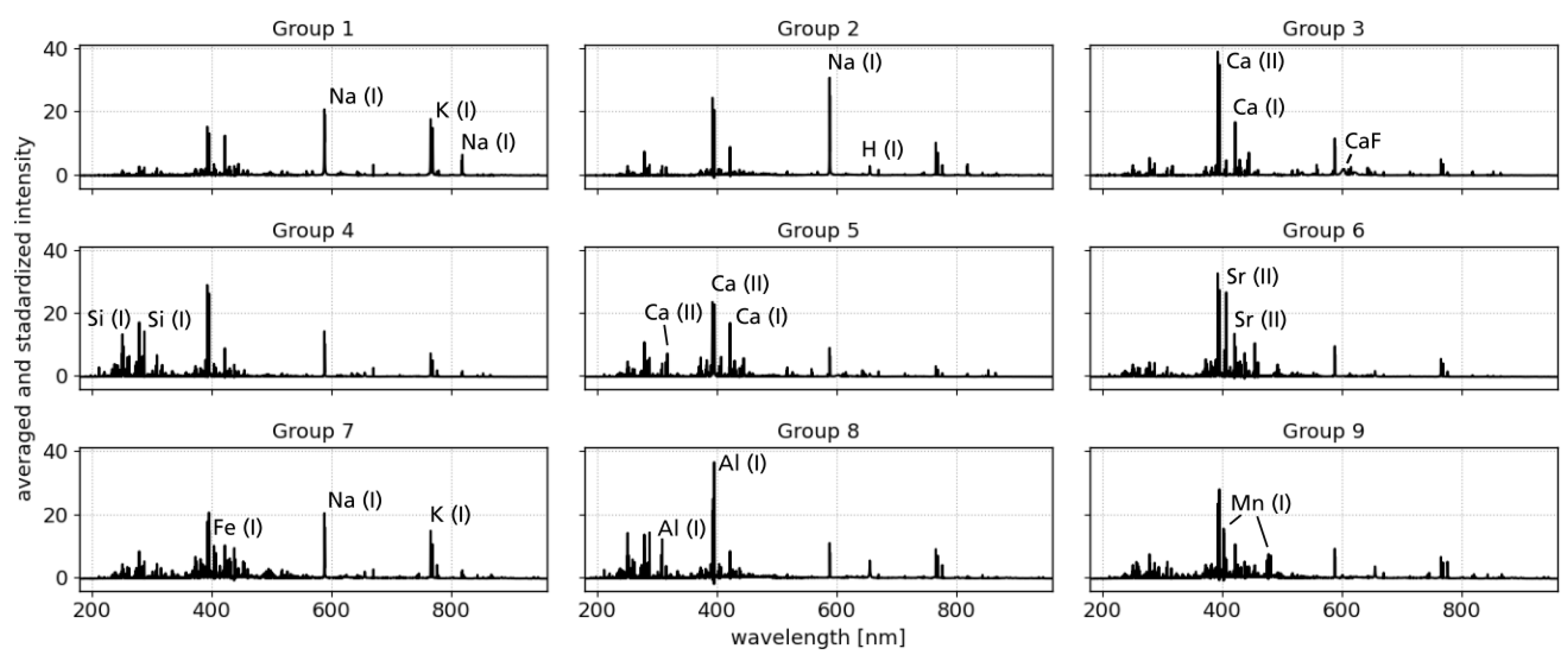
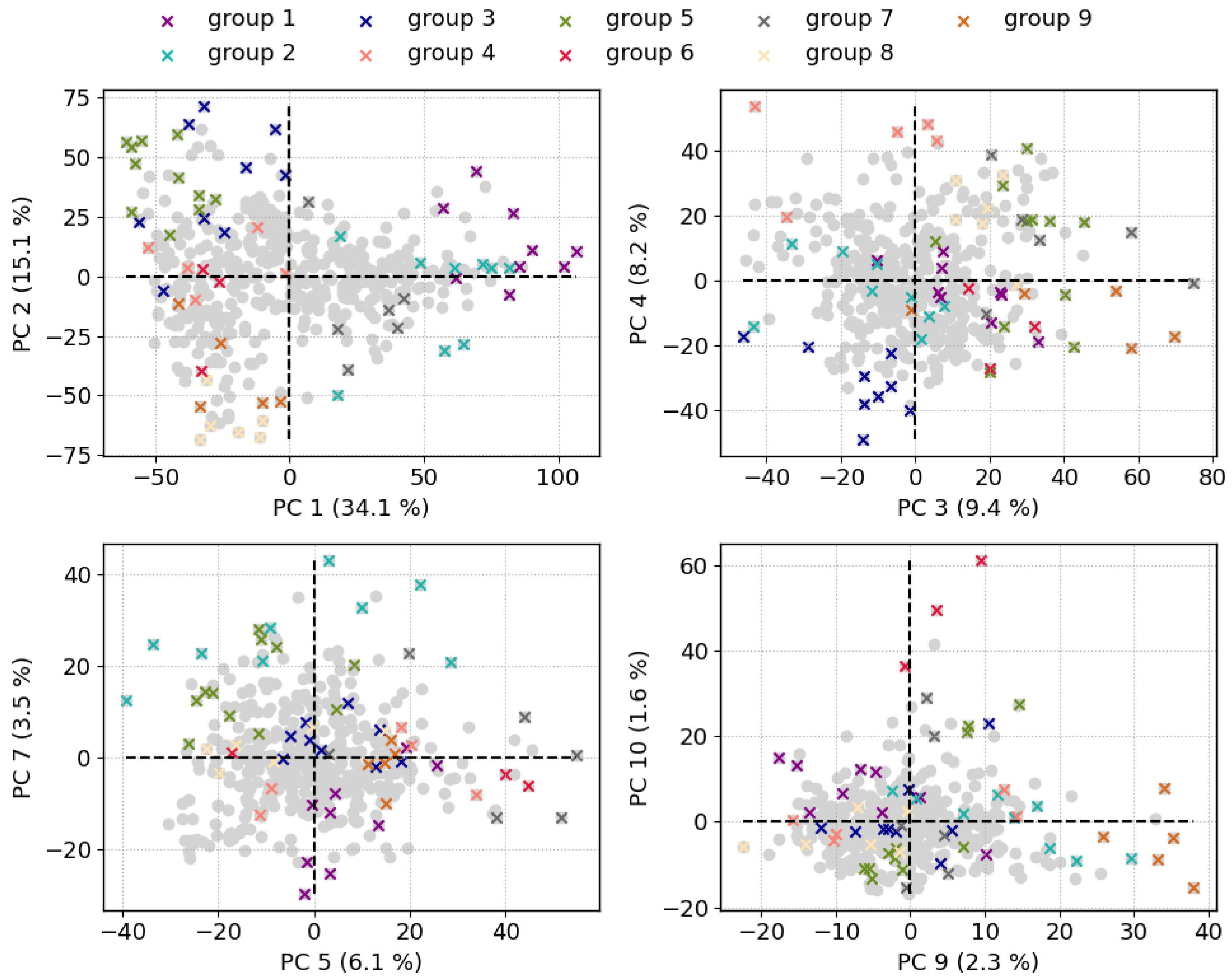
- PC 1 has positive correlations with emission lines from alkali elements, such as Li, Na, and K. The members of the IFF groups 1 and 2 and to a lesser extent also group 7 have mainly positive scores on PC 1 which is in agreement with their mean spectra showing strong emission lines of these elements.
- PC 2 is dominated by positive correlations with Ca emission lines and negative correlations with Al lines. In PCA space, PC 2 separates the IFF groups 3 and 5 from groups 8 and 9. In particular, the mean spectrum of group 8 shows strong lines of aluminum, whereas the mean spectra of group 3 and 5 show distinct lines of Ca.
- PC 4 has the strongest positive correlation with Si lines but also with Li and Mg. Compared to other components, PC 4 has a strong anti-correlation with the molecular emission band of CaF. Regarding the IFF groups, PC 4 splits groups 3 and 4 apart, which is consistent when looking at the mean spectra and the already discussed correlations.
- PC 5 is positively correlated with Fe emission lines, mainly neutral ones, and the K emission lines. Regarding the scores on PC 5, the main observation is that group 7 spectra have solely positive values and also the largest ones. This agrees with Fe emission lines in the mean spectrum of group 7. However, the mean spectrum has similar strong Na emission as K emission, although they are anti-correlated on PC 5.
- PC 7 separates the IFF groups 1 and 2 which are both dominated by emission lines of alkali elements. What distinguishes the two is evident on PC 7: emissions from Li and K are anti-correlated whereas those from Na have a positive correlation with PC 7. The scores of group 1 are negative and indeed the mean spectrum of group 1 also shows stronger lines of K than that of group 2.
- PC 9 is notable for positive correlations with Mn emission lines. This is in excellent agreement with the mean spectrum of group 9, whose members all have positive scores on PC 9.
- PC 10 also shows clear correlations here with emission lines of Sr. This is matched by the members of group 6, who all show strong Sr lines and at the same time have positive score values on PC 10.
6. Discussion
7. Summary and Conclusions
Author Contributions
Funding
Data Availability Statement
Conflicts of Interest
Abbreviations
| LIBS | Laser-induced breakdown spectroscopy |
| MSL | Mars Science Laboratory |
| IFF | Interesting features finder |
| IFFs | Interesting features finder spectra |
| PCA | Principal component analysis |
| PC | Principal component |
References
- Hahn, D.W.; Omenetto, N. Laser-Induced Breakdown Spectroscopy (LIBS), Part I: Review of Basic Diagnostics and Plasma—Particle Interactions: Still-Challenging Issues within the Analytical Plasma Community. Appl. Spectrosc. 2010, 64, 335A–336A. [Google Scholar] [CrossRef] [PubMed] [Green Version]
- Anabitarte, F.; Cobo, A.; Lopez-Higuera, J.M. Laser-Induced Breakdown Spectroscopy: Fundamentals, Applications, and Challenges. ISRN Spectrosc. 2012, 2012, 285240. [Google Scholar] [CrossRef] [Green Version]
- Hahn, D.W.; Omenetto, N. Laser-Induced Breakdown Spectroscopy (LIBS), Part II: Review of Instrumental and Methodological Approaches to Material Analysis and Applications to Different Fields. Appl. Spectrosc. 2012, 66, 347–419. [Google Scholar] [CrossRef] [PubMed]
- Harmon, R.S.; Russo, R.E.; Hark, R.R. Applications of laser-induced breakdown spectroscopy for geochemical and environmental analysis: A comprehensive review. Spectrochim. Acta Part B At. Spectrosc. 2013, 87, 11–26. [Google Scholar] [CrossRef]
- Fabre, C. Advances in Laser-Induced Breakdown Spectroscopy analysis for geology: A critical review. Spectrochim. Acta Part B At. Spectrosc. 2020, 166, 105799. [Google Scholar] [CrossRef]
- Senesi, G.S.; Harmon, R.S.; Hark, R.R. Field-portable and handheld laser-induced breakdown spectroscopy: Historical review, current status and future prospects. Spectrochim. Acta Part B At. Spectrosc. 2021, 175, 106013. [Google Scholar] [CrossRef]
- El Haddad, J.; Canioni, L.; Bousquet, B. Good practices in LIBS analysis: Review and advices. Spectrochim. Acta Part B At. Spectrosc. 2014, 101, 171–182. [Google Scholar] [CrossRef] [Green Version]
- Li, L.N.; Liu, X.F.; Yang, F.; Xu, W.M.; Wang, J.Y.; Shu, R. A review of artificial neural network based chemometrics applied in laser-induced breakdown spectroscopy analysis. Spectrochim. Acta Part B At. Spectrosc. 2021, 180, 106183. [Google Scholar] [CrossRef]
- Brunnbauer, L.; Gajarska, Z.; Lohninger, H.; Limbeck, A. A critical review of recent trends in sample classification using Laser-Induced Breakdown Spectroscopy (LIBS). TrAC Trends Anal. Chem. 2023, 159, 116859. [Google Scholar] [CrossRef]
- Palleschi, V. Chemometrics and Numerical Methods in LIBS; Wiley Online Library: Hoboken, NJ, USA, 2023. [Google Scholar]
- Forni, O.; Maurice, S.; Gasnault, O.; Wiens, R.C.; Cousin, A.; Clegg, S.M.; Sirven, J.B.; Lasue, J. Independent component analysis classification of laser induced breakdown spectroscopy spectra. Spectrochim. Acta Part B At. Spectrosc. 2013, 86, 31–41. [Google Scholar] [CrossRef]
- Pauca, V.P.; Piper, J.; Plemmons, R.J. Nonnegative matrix factorization for spectral data analysis. Linear Algebra Its Appl. 2006, 416, 29–47. [Google Scholar] [CrossRef] [Green Version]
- Lever, J.; Krzywinski, M.; Altman, N. Principal component analysis. Nat. Methods 2017, 14, 641–642. [Google Scholar] [CrossRef] [Green Version]
- Pořízka, P.; Klus, J.; Képeš, E.; Prochazka, D.; Hahn, D.W.; Kaiser, J. On the utilization of principal component analysis in laser-induced breakdown spectroscopy data analysis, a review. Spectrochim. Acta Part B At. Spectrosc. 2018, 148, 65–82. [Google Scholar] [CrossRef]
- Cousin, A.; Meslin, P.; Wiens, R.; Rapin, W.; Mangold, N.; Fabre, C.; Gasnault, O.; Forni, O.; Tokar, R.; Ollila, A.; et al. Compositions of coarse and fine particles in martian soils at gale: A window into the production of soils. Icarus 2015, 249, 22–42. [Google Scholar] [CrossRef]
- Gasnault, O.; Anderson, R.B.; Forni, O.; Maurice, S.; Wiens, R.C.; Pinet, P. Classification of ChemCam Targets Along the Traverse of Curiosity at Gale. In Proceedings of the Eighth International Conference on Mars, Pasadena, CA, USA, 14–18 July 2014; Lunar and Planetary Institute: Houston, TX, USA, 2014; p. Abstract #1269. [Google Scholar]
- Rammelkamp, K.; Gasnault, O.; Forni, O.; Bedford, C.C.; Dehouck, E.; Cousin, A.; Lasue, J.; David, G.; Gabriel, T.S.J.; Maurice, S.; et al. Clustering Supported Classification of ChemCam Data From Gale Crater, Mars. Earth Space Sci. 2021, 8, e2021EA001903. [Google Scholar] [CrossRef]
- Maurice, S.; Wiens, R.C.; Saccoccio, M.; Barraclough, B.; Gasnault, O.; Forni, O.; Mangold, N.; Baratoux, D.; Bender, S.; Berger, G.; et al. The ChemCam Instrument Suite on the Mars Science Laboratory (MSL) Rover: Science Objectives and Mast Unit Description. Space Sci. Rev. 2012, 170, 95–166. [Google Scholar] [CrossRef]
- Wiens, R.C.; Maurice, S.; Barraclough, B.; Saccoccio, M.; Barkley, W.C.; Bell, J.F.; Bender, S.; Bernardin, J.; Blaney, D.; Blank, J.; et al. The ChemCam Instrument Suite on the Mars Science Laboratory (MSL) Rover: Body Unit and Combined System Tests. Space Sci. Rev. 2012, 170, 167–227. [Google Scholar] [CrossRef]
- Maurice, S.; Wiens, R.C.; Bernardi, P.; Caïs, P.; Robinson, S.; Nelson, T.; Gasnault, O.; Reess, J.M.; Deleuze, M.; Rull, F.; et al. The SuperCam Instrument Suite on the Mars 2020 Rover: Science Objectives and Mast-Unit Description. Space Sci. Rev. 2021, 217, 47. [Google Scholar] [CrossRef]
- Wiens, R.C.; Maurice, S.; Robinson, S.H.; Nelson, A.E.; Cais, P.; Bernardi, P.; Newell, R.T.; Clegg, S.; Sharma, S.K.; Storms, S.; et al. The SuperCam Instrument Suite on the NASA Mars 2020 Rover: Body Unit and Combined System Tests. Space Sci. Rev. 2021, 217, 4. [Google Scholar] [CrossRef]
- Xu, W.; Liu, X.; Yan, Z.; Li, L.; Zhang, Z.; Kuang, Y.; Jiang, H.; Yu, H.; Yang, F.; Liu, C.; et al. The MarSCoDe Instrument Suite on the Mars Rover of China’s Tianwen-1 Mission. Space Sci. Rev. 2021, 217, 64. [Google Scholar] [CrossRef]
- Maurice, S.; Clegg, S.M.; Wiens, R.C.; Gasnault, O.; Rapin, W.; Forni, O.; Cousin, A.; Sautter, V.; Mangold, N.; Le Deit, L.; et al. ChemCam activities and discoveries during the nominal mission of the Mars Science Laboratory in Gale crater, Mars. J. Anal. At. Spectrom. 2016, 31, 863–889. [Google Scholar] [CrossRef] [Green Version]
- Gasnault, O.; Lanza, N.L.; Wiens, R.C.; Maurice, S.; Mangold, N.; Johnson, J.R.; Dehouck, E.; Beck, P.; Cousin, A.; Pinet, P.; et al. ChemCam: Zapping Mars for 10 Years (and More). In Proceedings of the 54th Lunar and Planetary Science Conference, The Woodlands, TX, USA, 13–17 March 2023; Lunar and Planetary Institute: Houston, TX, USA, 2023; p. Abstract #2076. [Google Scholar]
- Lasue, J.; Wiens, R.C.; Stepinski, T.F.; Forni, O.; Clegg, S.M.; Maurice, S. Nonlinear mapping technique for data visualization and clustering assessment of LIBS data: Application to ChemCam data. Anal. Bioanal. Chem. 2011, 400, 3247–3260. [Google Scholar] [CrossRef] [PubMed]
- Unnithan, V.; Sohl, F.; Thomsen, L. Vulcano Summer School 2019: Field-based terrestrial, marine and planetary analogue studies. In Proceedings of the EPSC-DPS Joint Meeting 2019, Geneva, Switzerland, 15–20 September 2019; Volume 2019, p. EPSC–DPS2019. [Google Scholar]
- Wu, Q.; Marina-Montes, C.; Cáceres, J.O.; Anzano, J.; Motto-Ros, V.; Duponchel, L. Interesting features finder (IFF): Another way to explore spectroscopic imaging data sets giving minor compounds and traces a chance to express themselves. Spectrochim. Acta Part B At. Spectrosc. 2022, 195, 106508. [Google Scholar] [CrossRef]
- Rammelkamp, K.; Schröder, S.; Ortenzi, G.; Pisello, A.; Stephan, K.; Baqué, M.; Hübers, H.W.; Forni, O.; Sohl, F.; Thomsen, L.; et al. Field investigation of volcanic deposits on Vulcano, Italy using a handheld laser-induced breakdown spectroscopy instrument. Spectrochim. Acta Part B At. Spectrosc. 2021, 177, 106067. [Google Scholar] [CrossRef]
- Iida, Y. Effects of atmosphere on laser vaporization and excitation processes of solid samples. Spectrochim. Acta Part B At. Spectrosc. 1990, 45, 1353–1367. [Google Scholar] [CrossRef]
- Peccerillo, A. Plio-Quaternary Volcanism in Italy; Springer: Berlin/Heidelberg, Germany, 2005; Volume 365. [Google Scholar]
- Rossi, S.; Petrelli, M.; Morgavi, D.; Vetere, F.P.; Almeev, R.R.; Astbury, R.L.; Perugini, D. Role of magma mixing in the pre-eruptive dynamics of the Aeolian Islands volcanoes (Southern Tyrrhenian Sea, Italy). Lithos 2019, 324–325, 165–179. [Google Scholar] [CrossRef]
- De Astis, G.; Lucchi, F.; Dellino, P.; La Volpe, L.; Tranne, C.A.; Frezzotti, M.L.; Peccerillo, A. Chapter 11 Geology, volcanic history and petrology of Vulcano (central Aeolian archipelago). Geol. Soc. Lond. Mem. 2013, 37, 281–349. [Google Scholar] [CrossRef]
- Fusillo, R.; Di Traglia, F.; Gioncada, A.; Pistolesi, M.; Wallace, P.J.; Rosi, M. Deciphering post-caldera volcanism: Insight into the Vulcanello (Island of Vulcano, Southern Italy) eruptive activity based on geological and petrological constraints. Bull. Volcanol. 2015, 77, 76. [Google Scholar] [CrossRef]
- Pisello, A.; De Angelis, S.; Ferrari, M.; Porreca, M.; Vetere, F.P.; Behrens, H.; De Sanctis, M.C.; Perugini, D. Visible and near-InfraRed (VNIR) reflectance of silicate glasses: Characterization of a featureless spectrum and implications for planetary geology. Icarus 2022, 374, 114801. [Google Scholar] [CrossRef]
- Piochi, M.; De Astis, G.; Petrelli, M.; Ventura, G.; Sulpizio, R.; Zanetti, A. Constraining the recent plumbing system of Vulcano (Aeolian Arc, Italy) by textural, petrological, and fractal analysis: The 1739 A.D. Pietre Cotte lava flow. Geochem. Geophys. Geosyst. 2009, 10, Q01009. [Google Scholar] [CrossRef]


| Site | # of LIBS Spectra Measured | # of LIBS Spectra after Outsorting |
|---|---|---|
| Valle dei Mostri | 39 | 32 |
| Vulcanello plateau | 32 | 28 |
| Pietre cotte lava flow | 123 | 123 |
| Grotta Palizzi bombs | 77 | 71 |
| Grotta Palizzi ashes | 64 | 41 |
| Monte Molineddo ashes | 116 | 113 |
| Piano Grotte dei Rossi ashes | 56 | 55 |
| Total | 507 | 463 |
Disclaimer/Publisher’s Note: The statements, opinions and data contained in all publications are solely those of the individual author(s) and contributor(s) and not of MDPI and/or the editor(s). MDPI and/or the editor(s) disclaim responsibility for any injury to people or property resulting from any ideas, methods, instructions or products referred to in the content. |
© 2023 by the authors. Licensee MDPI, Basel, Switzerland. This article is an open access article distributed under the terms and conditions of the Creative Commons Attribution (CC BY) license (https://creativecommons.org/licenses/by/4.0/).
Share and Cite
Rammelkamp, K.; Schröder, S.; Pisello, A.; Ortenzi, G.; Sohl, F.; Unnithan, V. Explorative Data Analysis Methods: Application to Laser-Induced Breakdown Spectroscopy Field Data Measured on the Island of Vulcano, Italy. Sensors 2023, 23, 6208. https://doi.org/10.3390/s23136208
Rammelkamp K, Schröder S, Pisello A, Ortenzi G, Sohl F, Unnithan V. Explorative Data Analysis Methods: Application to Laser-Induced Breakdown Spectroscopy Field Data Measured on the Island of Vulcano, Italy. Sensors. 2023; 23(13):6208. https://doi.org/10.3390/s23136208
Chicago/Turabian StyleRammelkamp, Kristin, Susanne Schröder, Alessandro Pisello, Gianluigi Ortenzi, Frank Sohl, and Vikram Unnithan. 2023. "Explorative Data Analysis Methods: Application to Laser-Induced Breakdown Spectroscopy Field Data Measured on the Island of Vulcano, Italy" Sensors 23, no. 13: 6208. https://doi.org/10.3390/s23136208