

Spatial Calibration of Humanoid Robot Flexible Tactile Skin for Human–Robot Interaction

 ,
,  , , , , and
Abstract
:1. Introduction
2. Related Works
2.1. Sense of Touch for Humanoid Robots
2.2. Flexible Tactile Skins
2.3. Tactile Sensor Calibration
3. Materials and Methods
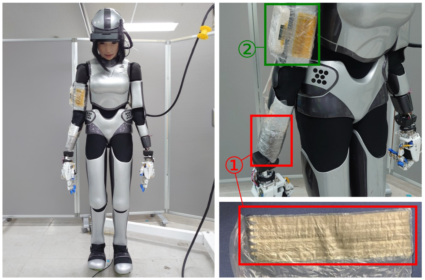
3.1. Flexible Tactile Sensor
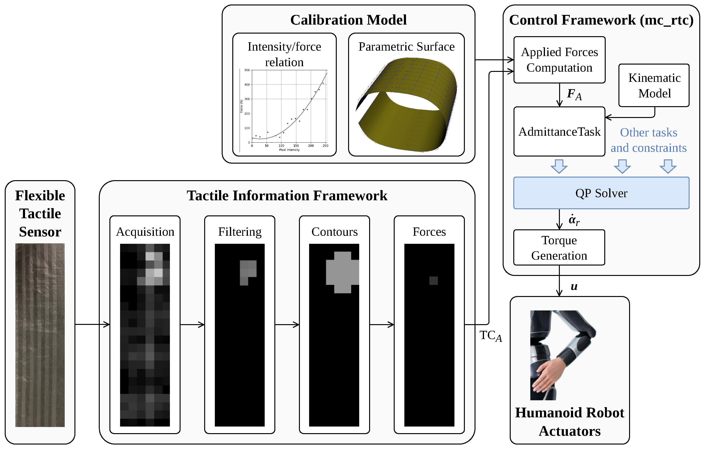
3.2. Tactile Information Framework
3.3. Control Framework
- The intensity/force relation, which is the relation between the intensity obtained with the acquisition software and the actual force applied. This relation is interpolated from experimental data.
- The spatial calibration model, which is the expression of the surface of the sensor as a B-spline surface. The method used to obtain the B-spline expression is detailed in the next subsection.
3.4. Spatial Calibration
3.4.1. Overview
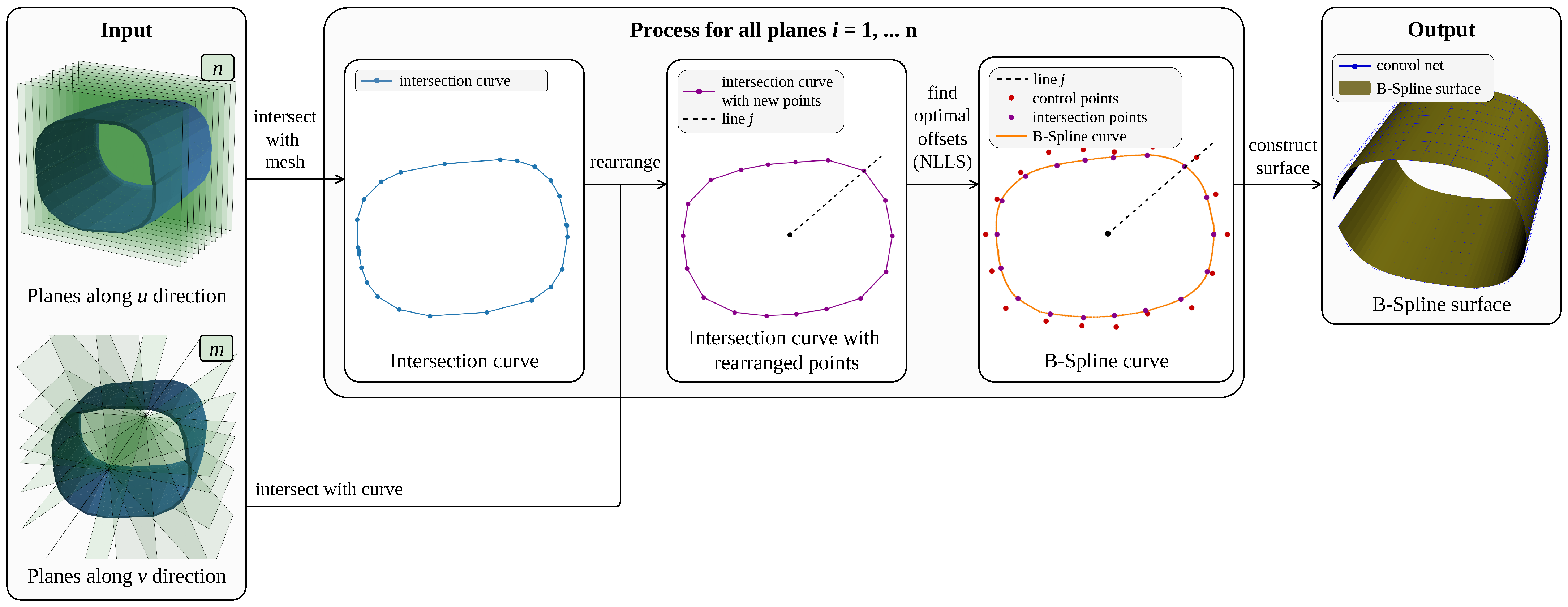
3.4.2. Inputs
3.4.3. Process
| Algorithm 1. Construction of the B-spline surface from a mesh and a tridimensional grid. | |
| Input: Integer , mesh , lists of planes and along u and v directions | |
| Output: B-spline surface | |
| 1: | ▹ List of B-spline curves |
| 2: | |
| 3: | |
| 4: for do | |
| 5: | ▹ List of curves |
| 6: | ▹ List of curves (2D) |
| 7: | ▹ List of lines (2D) |
| 8: | ▹ List of intersection points (2D) |
| 9: | ▹ List of control points (2D) |
| 10: | ▹ List of control points |
| 11: for do | |
| 12: | |
| 13: | |
| 14: | |
| 15: | |
| 16: end for | |
| 17: | |
| 18: end for | |
| 19: | |
3.4.4. Output
- The position of a cell is automatically given by evaluating the B-spline surface at parameters and .
- The normal vector to a cell can be computed using partial derivatives of the B-spline surface as:
3.5. Validation Experiment
3.5.1. Setup
- A support where an ATI Mini58 FTS, the robot right wrist, the tactile sensor and motion capture markers are mounted around the wrist. The relative positions of all these elements are known.
- A metal wand used to touch the tactile sensor, also with motion capture markers with known relative positions.
- A motion capture system composed of 10 Optitrack Prime 13 cameras.
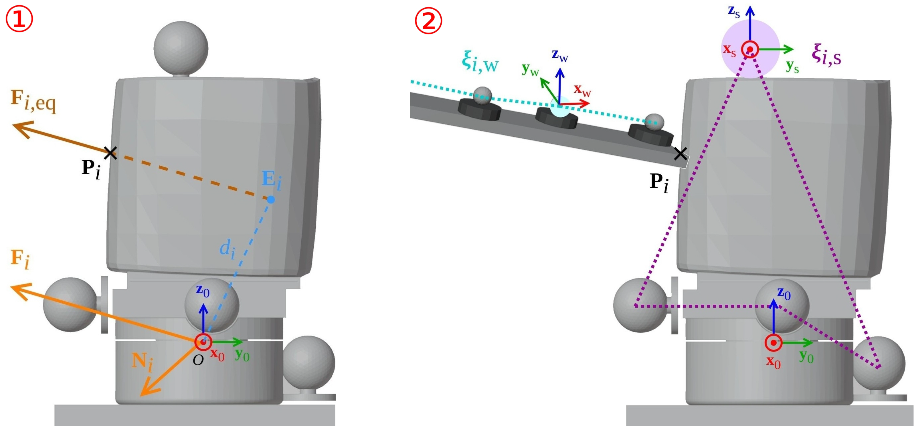
3.5.2. Using Force/Torque Sensor
3.5.3. Using Motion Capture
4. Results
4.1. B-Spline Surface Generation
- The planes along u direction are perpendicular to the main axis L and are separated with a constant distancewhere is the length of axis L crossing the convex hull on the mesh and a distance offset added to ensure that all the plane sections are complete.
- The planes along v direction cross on axis L and are separated with a constant angleBy construction, they are orthogonal to the planes .
4.2. Validation of Experimental Method
4.3. Validation of Spatial Calibration Method
4.3.1. Experimental Data
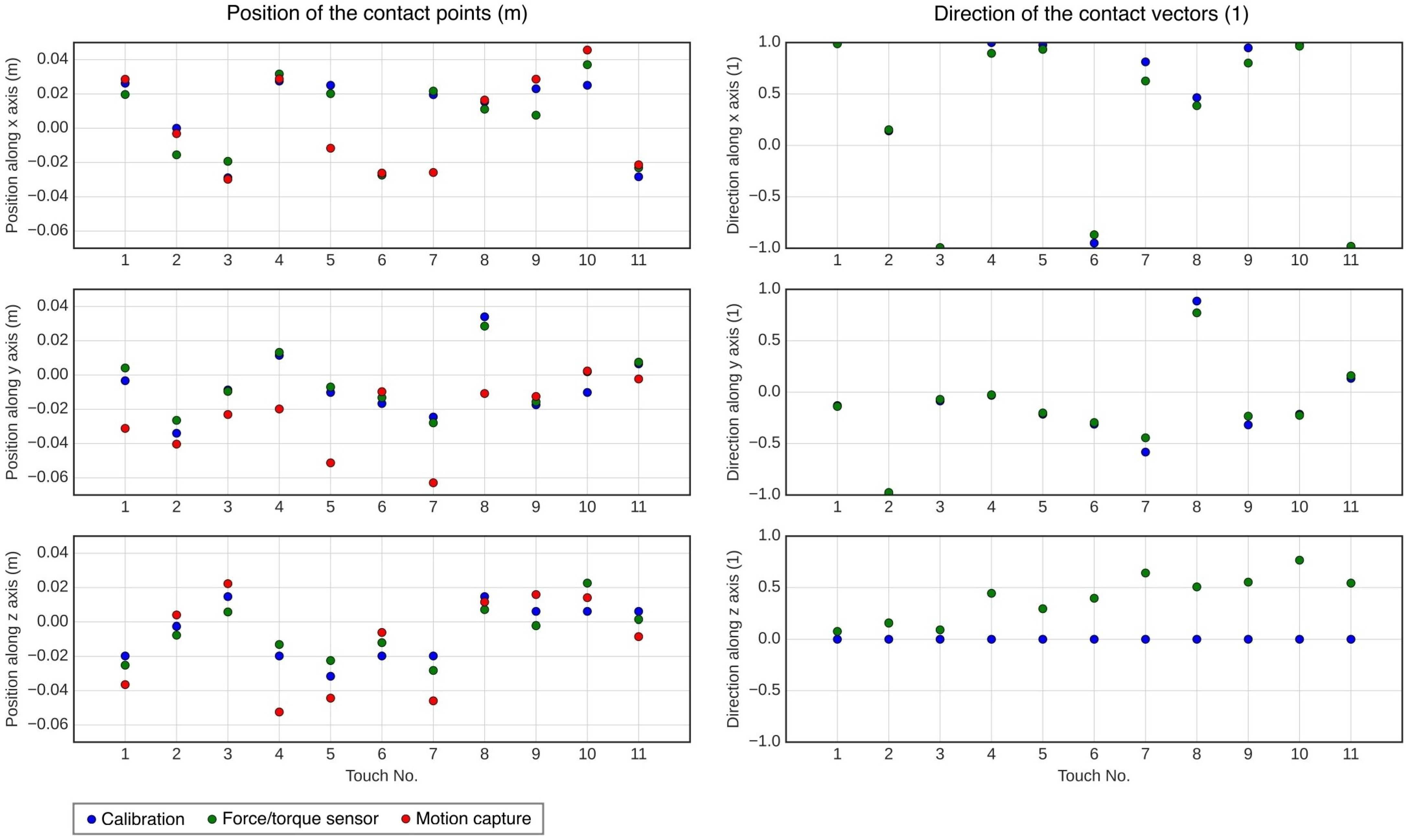
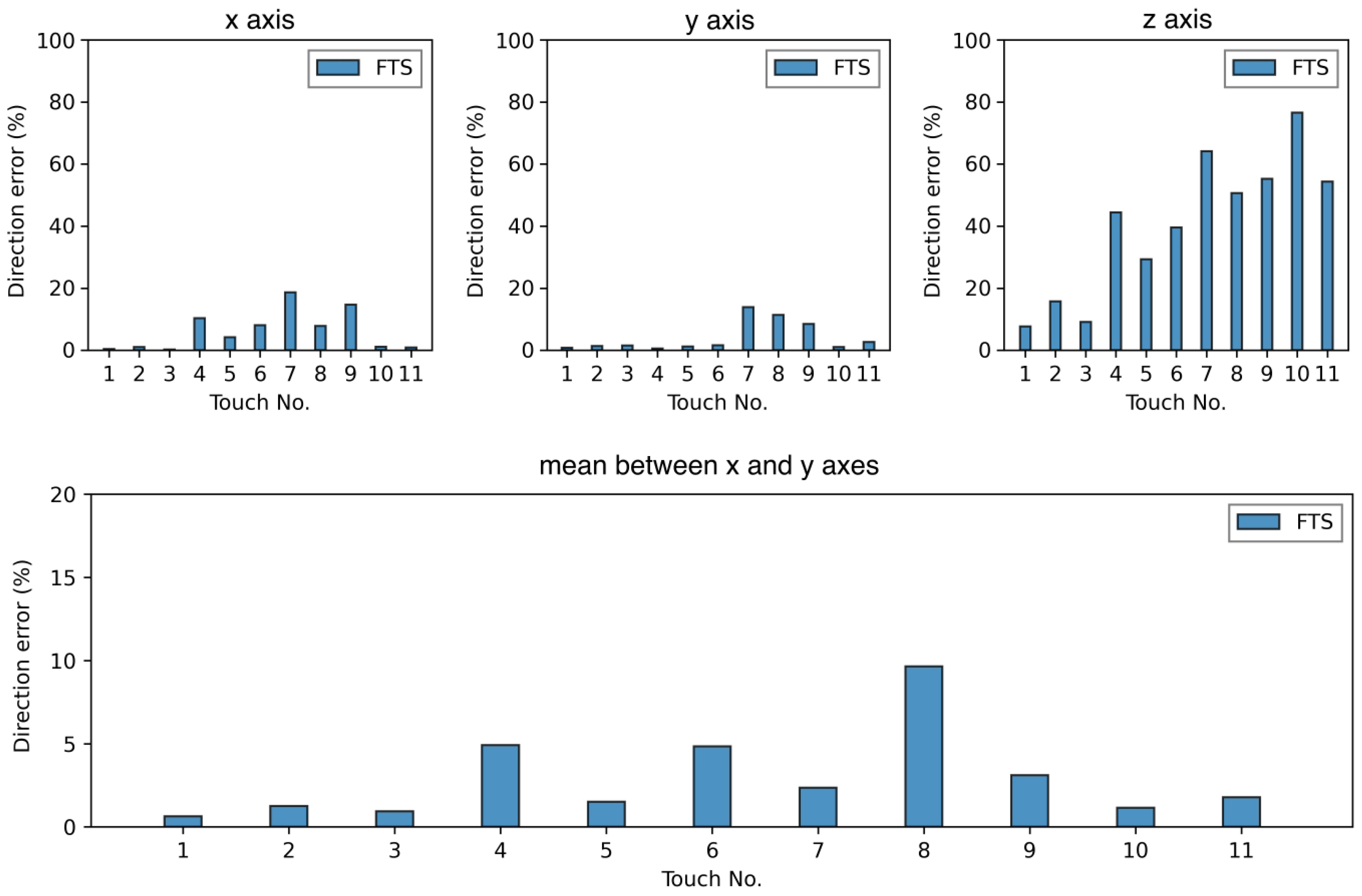
4.3.2. Validation of the Normals to the Cells
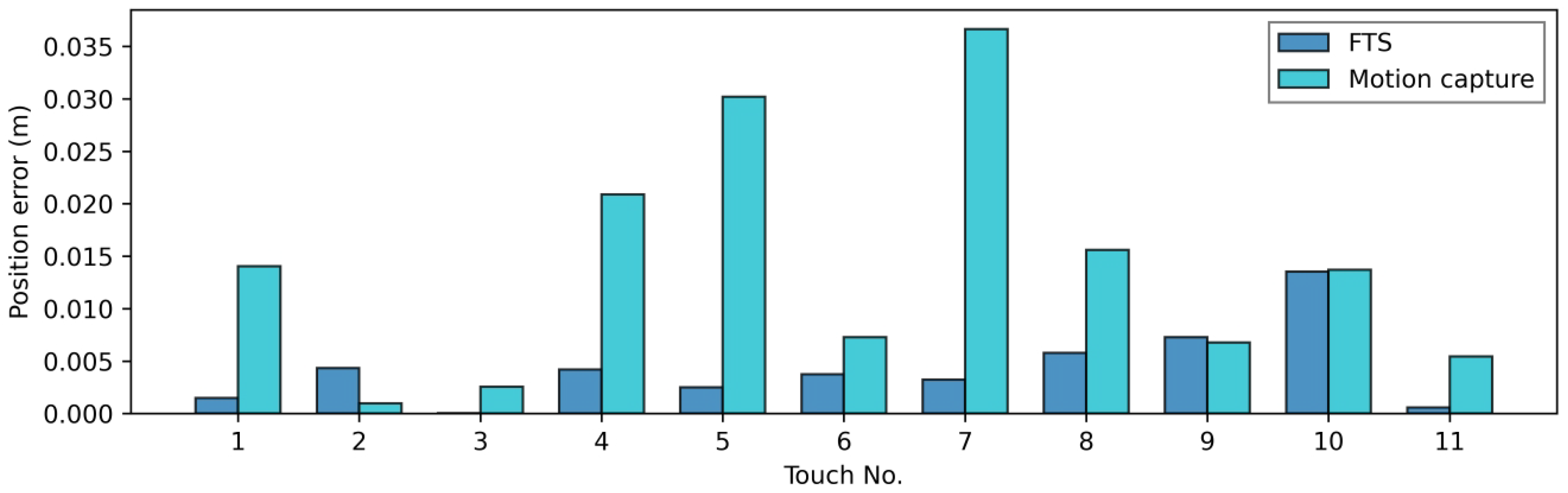
4.3.3. Validation of the Cell Positions
5. Discussion
6. Conclusions
Supplementary Materials
Author Contributions
Funding
Institutional Review Board Statement
Informed Consent Statement
Data Availability Statement
Conflicts of Interest
Abbreviations
| HRI | Human–Robot Interaction |
| pHRI | Physical Human–Robot Interaction |
| ROS | Robot Operating System |
| SPP | Serial Port Profile |
| TC | Tactile Contact |
| QP | Quadratic Programming |
| NLLS | Non-Linear Least Squares |
| NURBS | Non-Uniform Rational B-Spline |
| FTS | Force/Torque Sensor |
References
- Arents, J.; Abolins, V.; Judvaitis, J.; Vismanis, O.; Oraby, A.; Ozols, K. Human–Robot Collaboration Trends and Safety Aspects: A Systematic Review. J. Sens. Actuator Netw. 2021, 10, 48. [Google Scholar] [CrossRef]
- Podpora, M.; Gardecki, A.; Beniak, R.; Klin, B.; Vicario, J.L.; Kawala-Sterniuk, A. Human Interaction Smart Subsystem–Extending Speech-Based Human–robot Interaction Systems with an Implementation of External Smart Sensors. Sensors 2020, 20, 2376. [Google Scholar] [CrossRef] [PubMed]
- Zakia, U.; Menon, C. Human–Robot Collaboration in 3D via Force Myography Based Interactive Force Estimations Using Cross-Domain Generalization. IEEE Access 2022, 10, 35835–35845. [Google Scholar] [CrossRef]
- Darvish, K.; Penco, L.; Ramos, J.; Cisneros, R.; Pratt, J.; Yoshida, E.; Ivaldi, S.; Pucci, D. Teleoperation of Humanoid Robots: A Survey. arXiv 2023. [Google Scholar] [CrossRef]
- Madan, R.; Jenamani, R.K.; Nguyen, V.T.; Moustafa, A.; Hu, X.; Dimitropoulou, K.; Bhattacharjee, T. Sparcs: Structuring physically assistive robotics for caregiving with stakeholders-in-the-loop. In Proceedings of the 2022 IEEE/RSJ International Conference on Intelligent Robots and Systems (IROS), Kyoto, Japan, 23–27 October 2022; pp. 641–648. [Google Scholar]
- Fan, X.; Lee, D.; Jackel, L.; Howard, R.; Lee, D.; Isler, V. Enabling Low-Cost Full Surface Tactile Skin for Human Robot Interaction. IEEE Robot. Autom. Lett. 2022, 7, 1800–1807. [Google Scholar] [CrossRef]
- Guo, W. Microfluidic 3D printing polyhydroxyalkanoates-based bionic skin for wound healing. Mater. Futur. 2022, 1, 015401. [Google Scholar] [CrossRef]
- Kaneko, K.; Kanehiro, F.; Morisawa, M.; Miura, K.; Nakaoka, S.; Kajita, S. Cybernetic human HRP-4C. In Proceedings of the 9th IEEE-RAS International Conference on Humanoid Robots, Paris, France, 7–10 December 2009; pp. 7–14. [Google Scholar] [CrossRef]
- Gao, S.; Dai, Y.; Nathan, A. Tactile and Vision Perception for Intelligent Humanoids. Adv. Intell. Syst. 2022, 4, 2100074. [Google Scholar] [CrossRef]
- Pyo, S.; Lee, J.; Bae, K.; Sim, S.; Kim, J. Recent Progress in Flexible Tactile Sensors for Human-Interactive Systems: From Sensors to Advanced Applications. Adv. Mater. 2021, 33, 2005902. [Google Scholar] [CrossRef]
- Shu, X.; Ni, F.; Fan, X.; Yang, S.; Liu, C.; Tu, B.; Liu, Y.; Liu, H. A versatile humanoid robot platform for dexterous manipulation and human–robot collaboration. CAAI Trans. Intell. Technol. 2022, 8, 1–15. [Google Scholar] [CrossRef]
- Wan, Y.; Wang, Y.; Guo, C.F. Recent progresses on flexible tactile sensors. Mater. Today Phys. 2017, 1, 61–73. [Google Scholar] [CrossRef]
- Nguyen, T.D.; Lee, J.S. Recent Development of Flexible Tactile Sensors and Their Applications. Sensors 2022, 22, 50. [Google Scholar] [CrossRef] [PubMed]
- Roberts, P.; Zadan, M.; Majidi, C. Soft Tactile Sensing Skins for Robotics. Curr. Robot. Rep. 2021, 2, 343–354. [Google Scholar] [CrossRef]
- Mittendorfer, P.; Cheng, G. Humanoid Multimodal Tactile-Sensing Modules. IEEE Trans. Robot. 2011, 27, 401–410. [Google Scholar] [CrossRef]
- Pang, G.; Deng, J.; Wang, F.; Zhang, J.; Pang, Z.; Yang, G. Development of Flexible Robot Skin for Safe and Natural Human–Robot Collaboration. Micromachines 2018, 9, 576. [Google Scholar] [CrossRef]
- Wu, H.; Zheng, B.; Wang, H.; Ye, J. New Flexible Tactile Sensor Based on Electrical Impedance Tomography. Micromachines 2022, 13, 185. [Google Scholar] [CrossRef]
- Lai, Q.T.; Sun, Q.J.; Tang, Z.; Tang, X.G.; Zhao, X.H. Conjugated Polymer-Based Nanocomposites for Pressure Sensors. Molecules 2023, 28, 1627. [Google Scholar] [CrossRef]
- Park, D.Y.; Joe, D.; Kim, D.H.; Park, H.; Han, J.H.; Jeong, C.K.; Park, H.; Park, J.; Joung, B.; Lee, K. Self-Powered Real-Time Arterial Pulse Monitoring Using Ultrathin Epidermal Piezoelectric Sensors. Adv. Mater. 2017, 29, 1702308. [Google Scholar] [CrossRef]
- Zhang, M.; Wang, Z.; Xu, H.; Chen, L.; Jin, Y.; Wang, W. Flexible Tactile Sensing Array with High Spatial Density Based on Parylene Mems Technique. In Proceedings of the 2023 IEEE 36th International Conference on Micro Electro Mechanical Systems (MEMS), Munich, Germany, 15–19 January 2023; pp. 243–246. [Google Scholar] [CrossRef]
- Bartlett, M.D.; Markvicka, E.J.; Tutika, R.; Majidi, C. Soft-matter damage detection systems for electronics and structures. In Proceedings of the Nondestructive Characterization and Monitoring of Advanced Materials, Aerospace, Civil Infrastructure, and Transportation XIII, Denver, CO, USA, 1 April 2019; Gyekenyesi, A.L., Ed.; International Society for Optics and Photonics, SPIE: Bellingham, WA, USA, 2019; Volume 10971, p. 1097112. [Google Scholar] [CrossRef]
- Kim, K.; Sim, M.; Lim, S.H.; Kim, D.; Lee, D.; Shin, K.; Moon, C.; Choi, J.W.; Jang, J.E. Tactile avatar: Tactile sensing system mimicking human tactile cognition. Adv. Sci. 2021, 8, 2002362. [Google Scholar] [CrossRef]
- Rustler, L.; Potocna, B.; Polic, M.; Stepanova, K.; Hoffmann, M. Spatial calibration of whole-body artificial skin on a humanoid robot: Comparing self-contact, 3D reconstruction, and CAD-based calibration. In Proceedings of the 20th IEEE-RAS International Conference on Humanoid Robots, Munich, Germany, 20–21 July 2021; pp. 445–452. [Google Scholar] [CrossRef]
- Lifton, J.; Liu, T.; McBride, J. Non-linear least squares fitting of Bézier surfaces to unstructured point clouds. AIMS Math. 2021, 6, 3142–3159. [Google Scholar] [CrossRef]
- Rodríguez, J.A.M. Efficient NURBS surface fitting via GA with SBX for free-form representation. Int. J. Comput. Integr. Manuf. 2017, 30, 981–994. [Google Scholar] [CrossRef]
- Liu, M.; Li, B.; Guo, Q.; Zhu, C.; Hu, P.; Shao, Y. Progressive iterative approximation for regularized least square bivariate B-spline surface fitting. J. Comput. Appl. Math. 2018, 327, 175–187. [Google Scholar] [CrossRef]
- Liu, X.; Huang, M.; Li, S.; Ma, C. Surfaces of Revolution (SORs) Reconstruction Using a Self-Adaptive Generatrix Line Extraction Method from Point Clouds. Remote Sens. 2019, 11, 1125. [Google Scholar] [CrossRef]
- Wang, S.; Xia, Y.; Wang, R.; You, L.; Zhang, J. Optimal NURBS conversion of PDE surface-represented high-speed train heads. Optim. Eng. 2019, 20, 907–928. [Google Scholar] [CrossRef]
- Sharma, G.; Liu, D.; Kalogerakis, E.; Maji, S.; Chaudhuri, S.; Měch, R. ParSeNet: A Parametric Surface Fitting Network for 3D Point Clouds. In Proceedings of the Computer Vision–ECCV 2020: 16th European Conference, Glasgow, UK, 23–28 August 2020. [Google Scholar] [CrossRef]
- Gao, J.; Tang, C.; Ganapathi-Subramanian, V.; Huang, J.; Su, H.; Guibas, L.J. Deepspline: Data-driven reconstruction of parametric curves and surfaces. arXiv 2019. [Google Scholar] [CrossRef]
- Ben-Shabat, Y.; Gould, S. DeepFit: 3D Surface Fitting via Neural Network Weighted Least Squares. In Proceedings of the Computer Vision–ECCV 2020: 16th European Conference, Glasgow, UK, 23–28 August 2020. [Google Scholar] [CrossRef]
- Nobeshima, T.; Uemura, S.; Yoshida, M.; Kamata, T. Stretchable conductor from oriented short conductive fibers for wiring soft electronics. Polym. Bull. 2016, 73, 2521–2529. [Google Scholar] [CrossRef]
- Quigley, M.; Conley, K.; Gerkey, B.; Faust, J.; Foote, T.; Leibs, J.; Wheeler, R.; Ng, A.Y. ROS: An open-source Robot Operating System. In Proceedings of the ICRA Workshop on Open Source Software, Kobe, Japan, 12–17 May 2009; Volume 3, p. 5. [Google Scholar]
- CNRS-AIST JRL; CNRS LIRMM. mc_rtc. Available online: https://jrl-umi3218.github.io/mc_rtc/index.html (accessed on 8 March 2023).
- Chi, C.; Sun, X.; Xue, N.; Li, T.; Liu, C. Recent Progress in Technologies for Tactile Sensors. Sensors 2018, 18, 948. [Google Scholar] [CrossRef] [PubMed]
- Kakani, V.; Cui, X.; Ma, M.; Kim, H. Vision-Based Tactile Sensor Mechanism for the Estimation of Contact Position and Force Distribution Using Deep Learning. Sensors 2021, 21, 1920. [Google Scholar] [CrossRef]
- Bradski, G. The OpenCV Library. Dr. Dobb’S J. Softw. Tools 2000, 25, 120–123. [Google Scholar]
- Woodall, W.; Harrison, J. Serial by wjwwood. Available online: http://wjwwood.io/serial/ (accessed on 8 March 2023).
- OpenCV: Miscellaneous Image Transformations: Adaptive Threshold. Available online: https://docs.opencv.org/3.1.0/d7/d1b/group__imgproc__misc.html#ga72b913f352e4a1b1b397736707afcde3 (accessed on 9 March 2023).
- Suzuki, S.; Abe, K. Topological structural analysis of digitized binary images by border following. Comput. Vis. Graph. Image Process. 1985, 30, 32–46. [Google Scholar] [CrossRef]
- CNRS-AIST JRL; CNRS LIRMM. Tutorials-Admittance Sample Controller—mc_rtc. Available online: https://jrl-umi3218.github.io/mc_rtc/tutorials/samples/sample-admittance.html (accessed on 13 March 2023).
- Dawson-Haggerty, M. trimesh. Available online: https://trimsh.org/ (accessed on 8 March 2023).
- Bingol, O.R.; Krishnamurthy, A. NURBS-Python: An open-source object-oriented NURBS modeling framework in Python. SoftwareX 2019, 9, 85–94. [Google Scholar] [CrossRef]
- Piegl, L.; Tiller, W. The NURBS Book, 2nd ed.; Springer: New York, NY, USA, 1996. [Google Scholar] [CrossRef]
- Bisect-Blender Manual. Available online: https://docs.blender.org/manual/en/2.80/modeling/meshes/editing/subdividing/bisect.html (accessed on 24 April 2023).
- Bingol, O.R. Splitting and Decomposition–NURBS-Python 5.3.1 Documentation. Available online: https://nurbs-python.readthedocs.io/en/5.x/visualization_splitting.html (accessed on 12 March 2023).
- Blender Documentation Team. Intersect (Boolean)–Blender Manual. Available online: https://docs.blender.org/manual/en/latest/modeling/meshes/editing/face/intersect_boolean.html (accessed on 9 March 2023).
- Cignoni, P.; Callieri, M.; Corsini, M.; Dellepiane, M.; Ganovelli, F.; Ranzuglia, G. MeshLab: An Open-Source Mesh Processing Tool. In Proceedings of the Eurographics Italian Chapter Conference, Salerno, Italy, 2–4 July 2008; Scarano, V., Chiara, R., Erra, U., Eds.; Volume 1, pp. 129–136. [Google Scholar] [CrossRef]
- Zatsiorsky, V.M. Kinetics of Human Motion; Human Kinetics: Champaign, IL, USA, 2002. [Google Scholar]
- ATI Industrial Automation. ATI Industrial Automation: F/T Sensor Mini58. Available online: https://www.ati-ia.com/products/ft/ft_models.aspx?id=Mini58 (accessed on 24 April 2023).
- OptiTrack Documentation. Available online: https://docs.optitrack.com/ (accessed on 23 March 2023).


| Property | Value | Comments |
|---|---|---|
| Dimensions | 6 × 22 cells | - |
| Cell size | 1 × 1 | - |
| Sensing modality | Capacitive | - |
| Young’s modulus | 13 MPa | For strains under 10% |
| Sensing ranges | 35–45 pF | Due to compression of the void layer in the sensor [32]. |
| 45–125 pF | Due to compression of the elastic body [32]. | |
| Sensitivity | 10 dgt./kPa | In the weak sensitivity range (35–45 pF). |
| Limit of detection | 200 kPa | In the strong sensitivity range (45–125 pF). |
| Response time | 100 ms | For an elastic ball hit against the sensor. See Figure S1 (2). |
| Recovery time | 5.1 s | For a 10 kPa load applied for 2 s. See Figure S1 (3). |
| Hysteresis | Not detected | Not detected with the applied loads. See Figure S1 (4,5). |
| Parameters | Geometric Distance (mm) | Hausdorff Distance (mm) | Generation | |||||
|---|---|---|---|---|---|---|---|---|
| n | m | min | max | mean | min | max | mean | time (ms) |
| 5 | 5 | 0.001 | 3.820 | 0.987 | 0.000 | 3.820 | 1.030 | 344 |
| 5 | 10 | 0.001 | 3.856 | 0.824 | 0.000 | 3.856 | 0.869 | 414 |
| 10 | 5 | 0.001 | 3.820 | 1.006 | 0.000 | 3.820 | 1.036 | 598 |
| 10 | 10 | 0.001 | 3.856 | 0.854 | 0.000 | 3.856 | 0.885 | 766 |
Disclaimer/Publisher’s Note: The statements, opinions and data contained in all publications are solely those of the individual author(s) and contributor(s) and not of MDPI and/or the editor(s). MDPI and/or the editor(s) disclaim responsibility for any injury to people or property resulting from any ideas, methods, instructions or products referred to in the content. |
© 2023 by the authors. Licensee MDPI, Basel, Switzerland. This article is an open access article distributed under the terms and conditions of the Creative Commons Attribution (CC BY) license (https://creativecommons.org/licenses/by/4.0/).
Share and Cite
Chefchaouni Moussaoui, S.; Cisneros-Limón, R.; Kaminaga, H.; Benallegue, M.; Nobeshima, T.; Kanazawa, S.; Kanehiro, F. Spatial Calibration of Humanoid Robot Flexible Tactile Skin for Human–Robot Interaction. Sensors 2023, 23, 4569. https://doi.org/10.3390/s23094569
Chefchaouni Moussaoui S, Cisneros-Limón R, Kaminaga H, Benallegue M, Nobeshima T, Kanazawa S, Kanehiro F. Spatial Calibration of Humanoid Robot Flexible Tactile Skin for Human–Robot Interaction. Sensors. 2023; 23(9):4569. https://doi.org/10.3390/s23094569
Chicago/Turabian StyleChefchaouni Moussaoui, Sélim, Rafael Cisneros-Limón, Hiroshi Kaminaga, Mehdi Benallegue, Taiki Nobeshima, Shusuke Kanazawa, and Fumio Kanehiro. 2023. "Spatial Calibration of Humanoid Robot Flexible Tactile Skin for Human–Robot Interaction" Sensors 23, no. 9: 4569. https://doi.org/10.3390/s23094569