
A Tunable Hyperspectral Imager for Detection and Quantification of Marine Biofouling on Coated Surfaces

 ,
,  , , , , , and
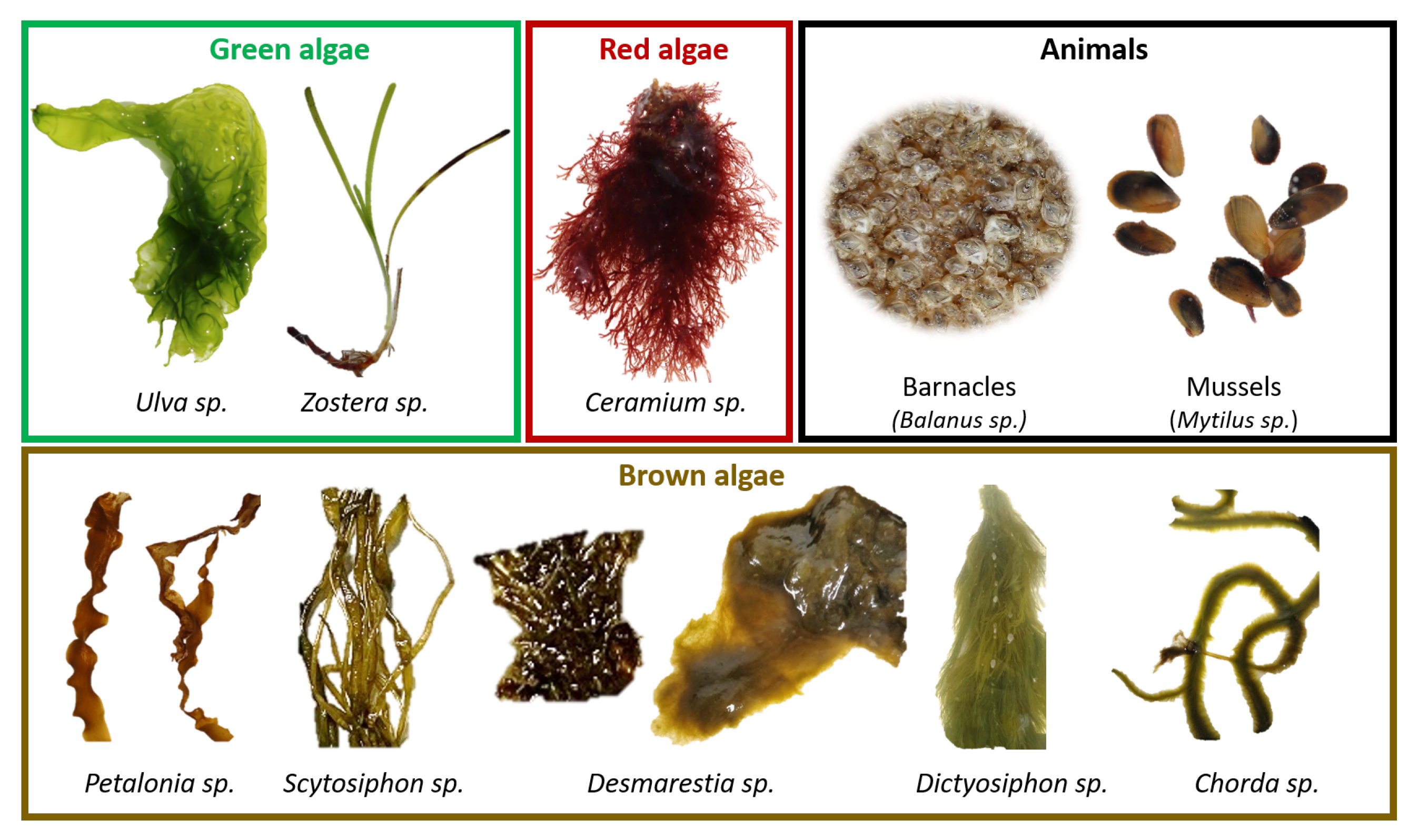
Abstract
:1. Introduction
2. Materials and Methods
2.1. Test Site and Materials
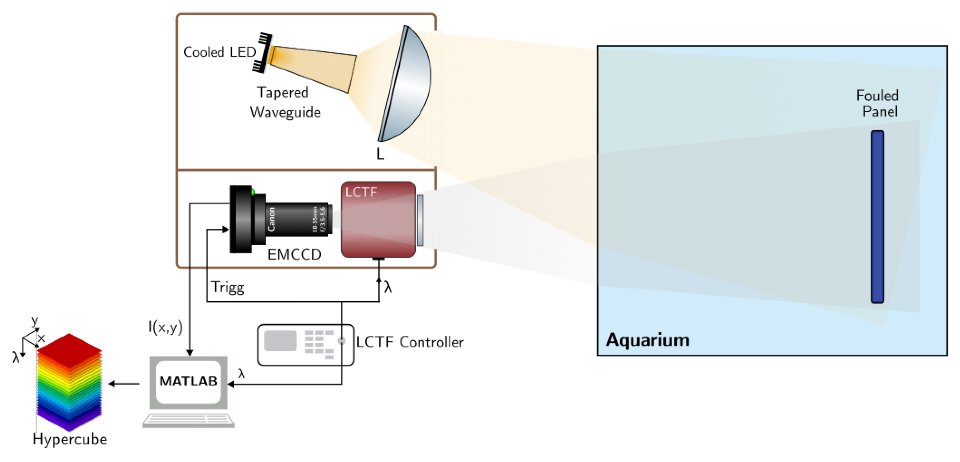
2.2. Sensor
2.2.1. Imaging Spectrometer
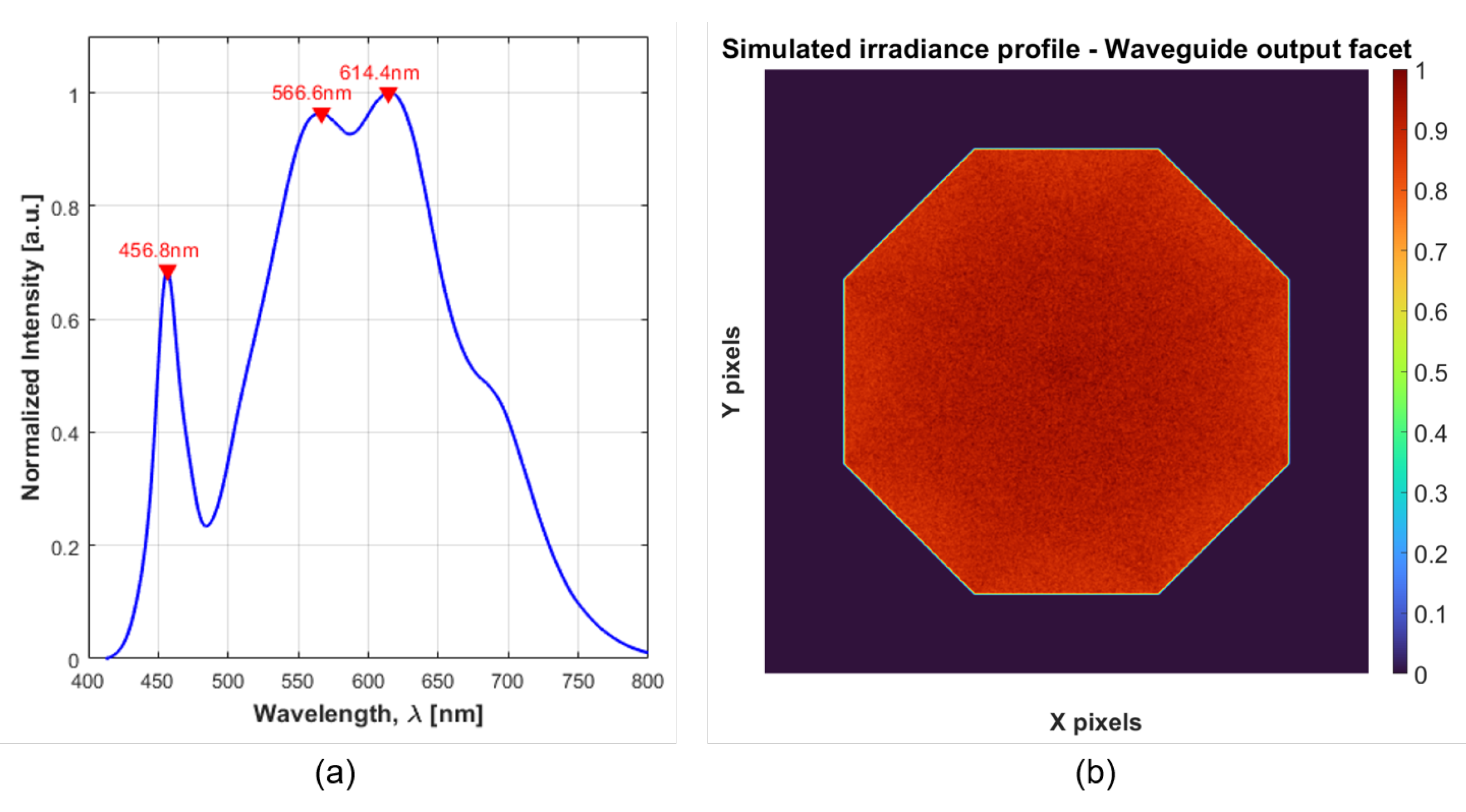
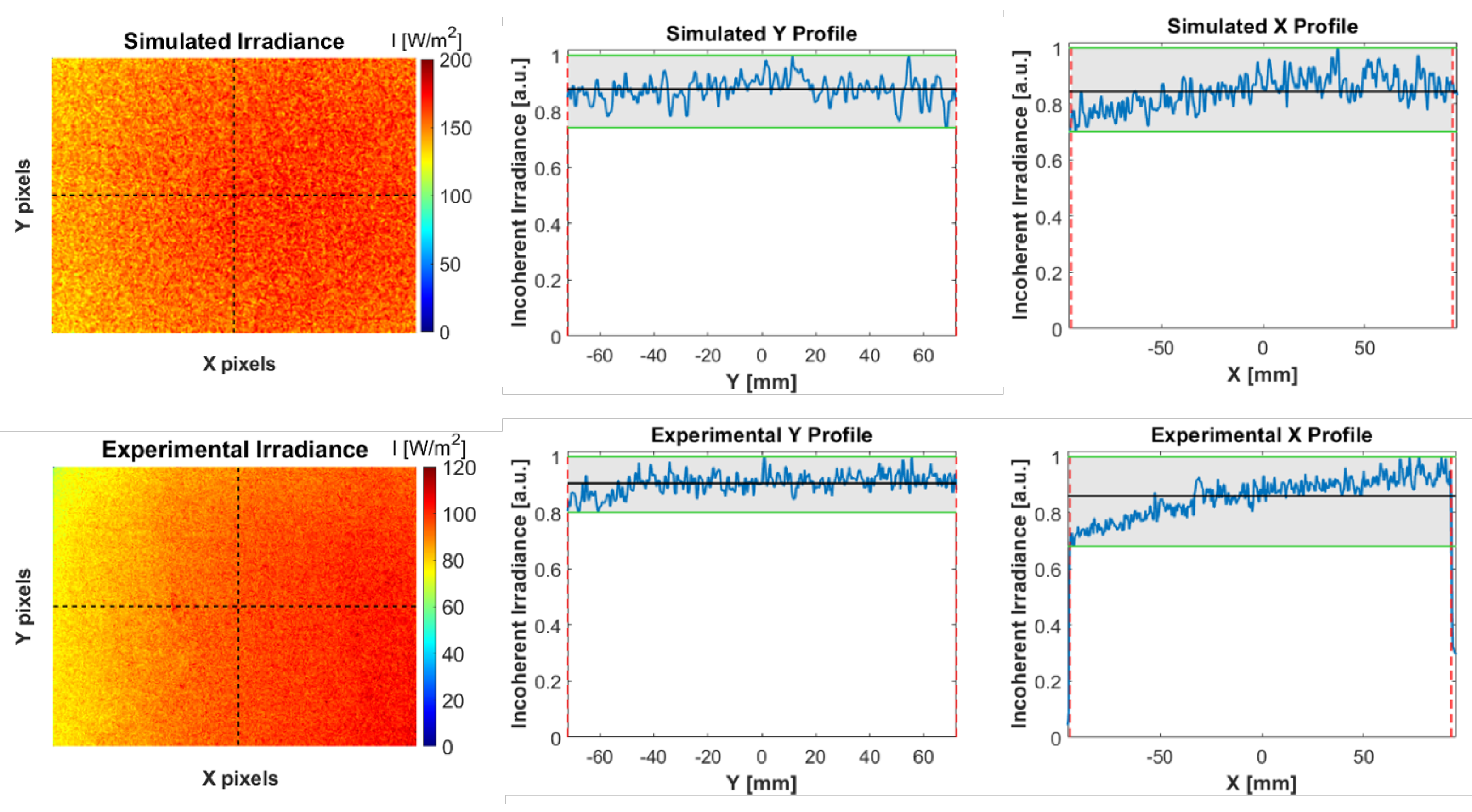
2.2.2. Led Illumination System
2.3. Data Acquisition
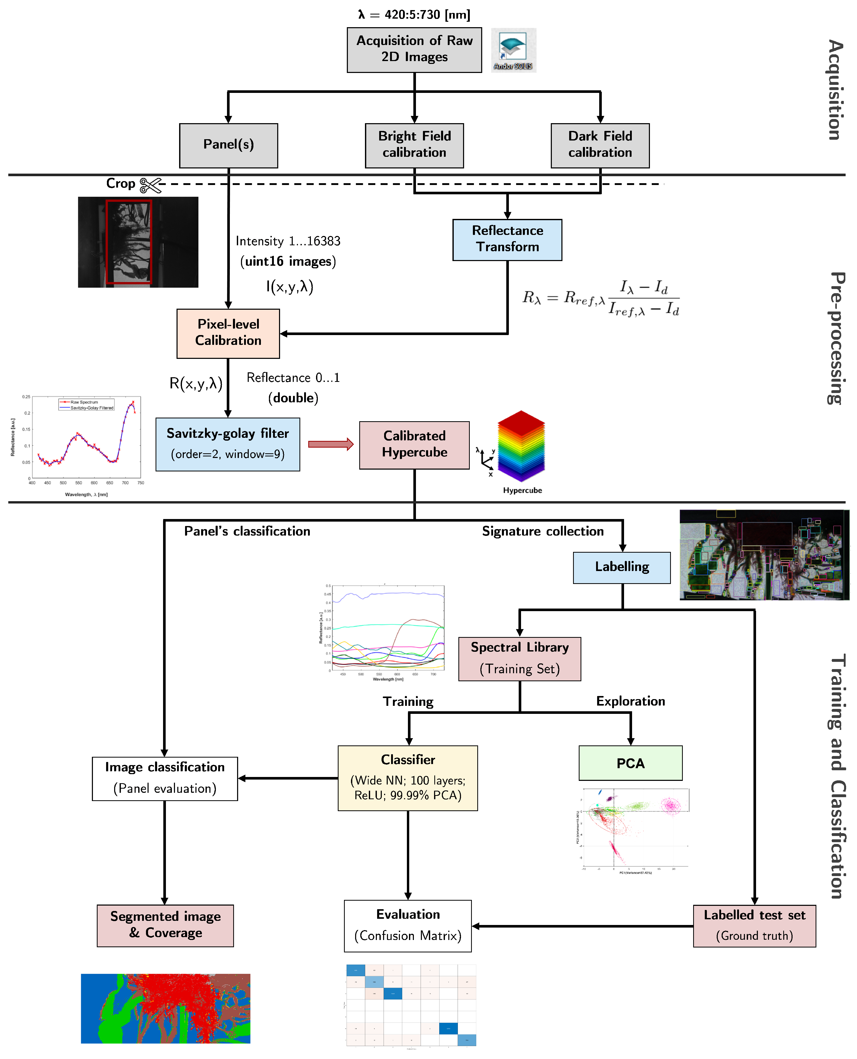
2.4. Spectral Data Processing and Analysis
2.4.1. Pre-Processing and Reflectance Transform
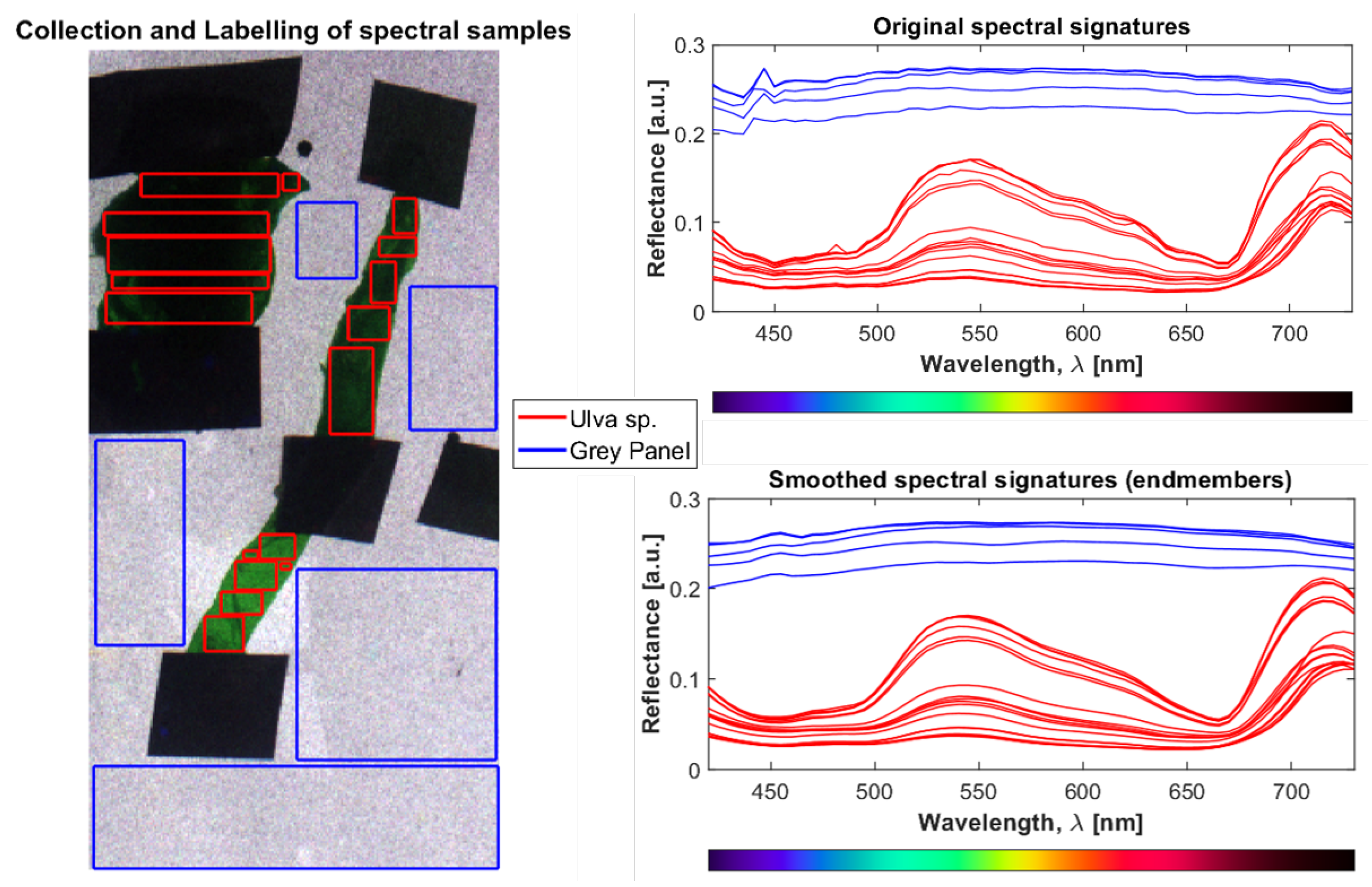
2.4.2. Signature Collection (Training Set)
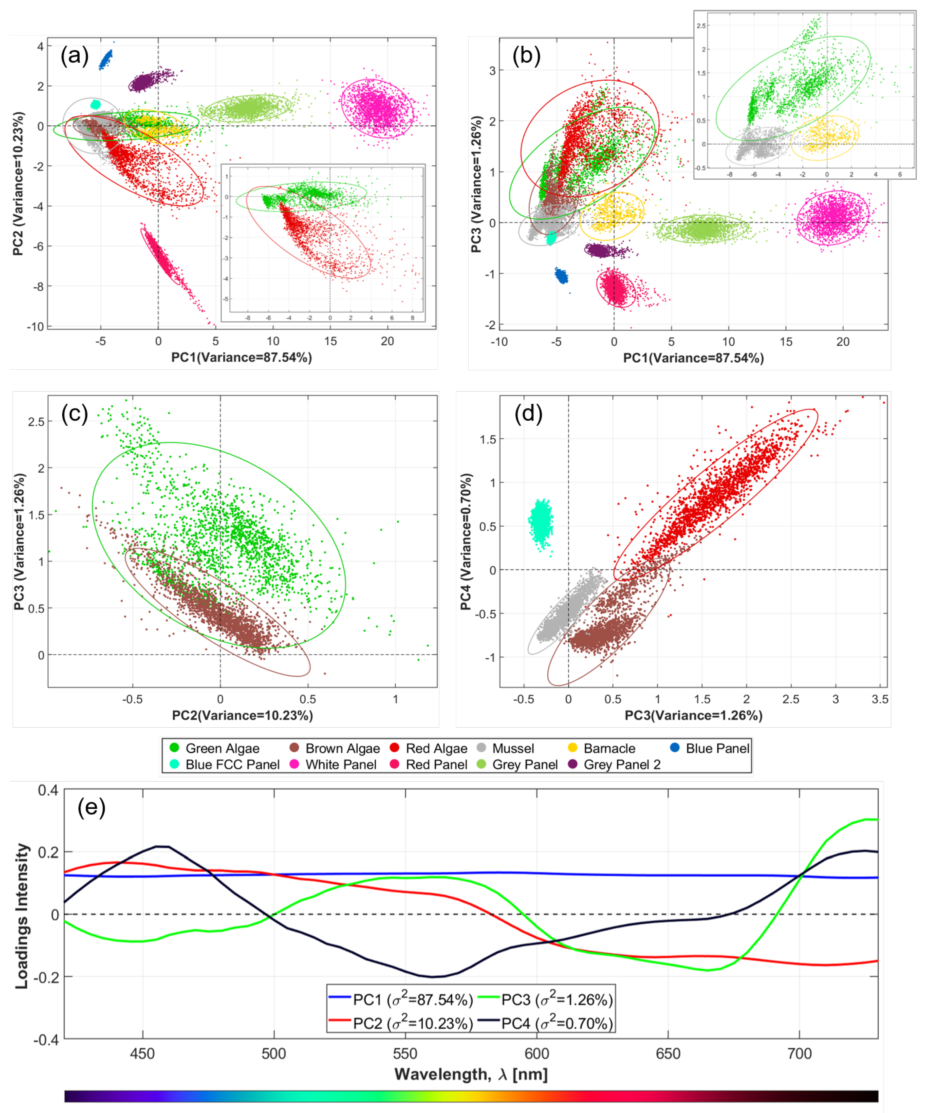
2.4.3. Principal Component Analysis
2.4.4. Classification: Neural Network
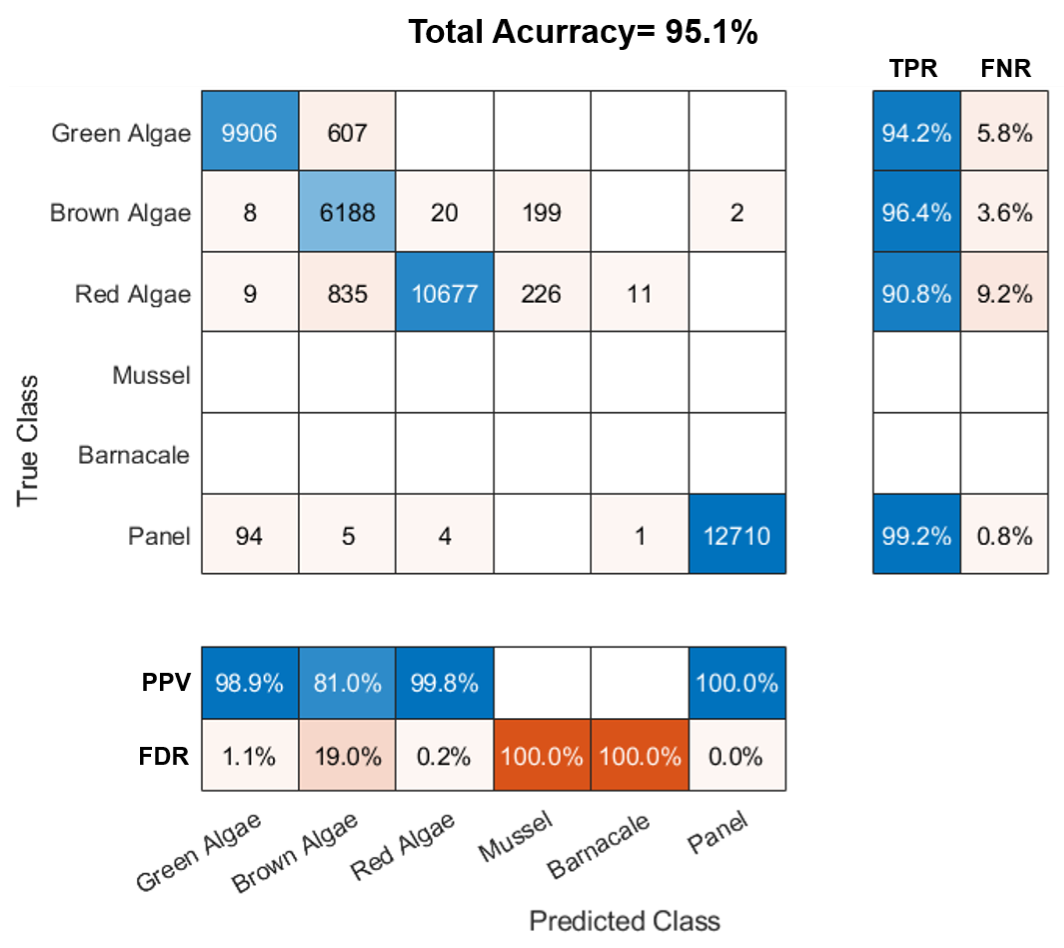
2.4.5. Testing and Classification Accuracy
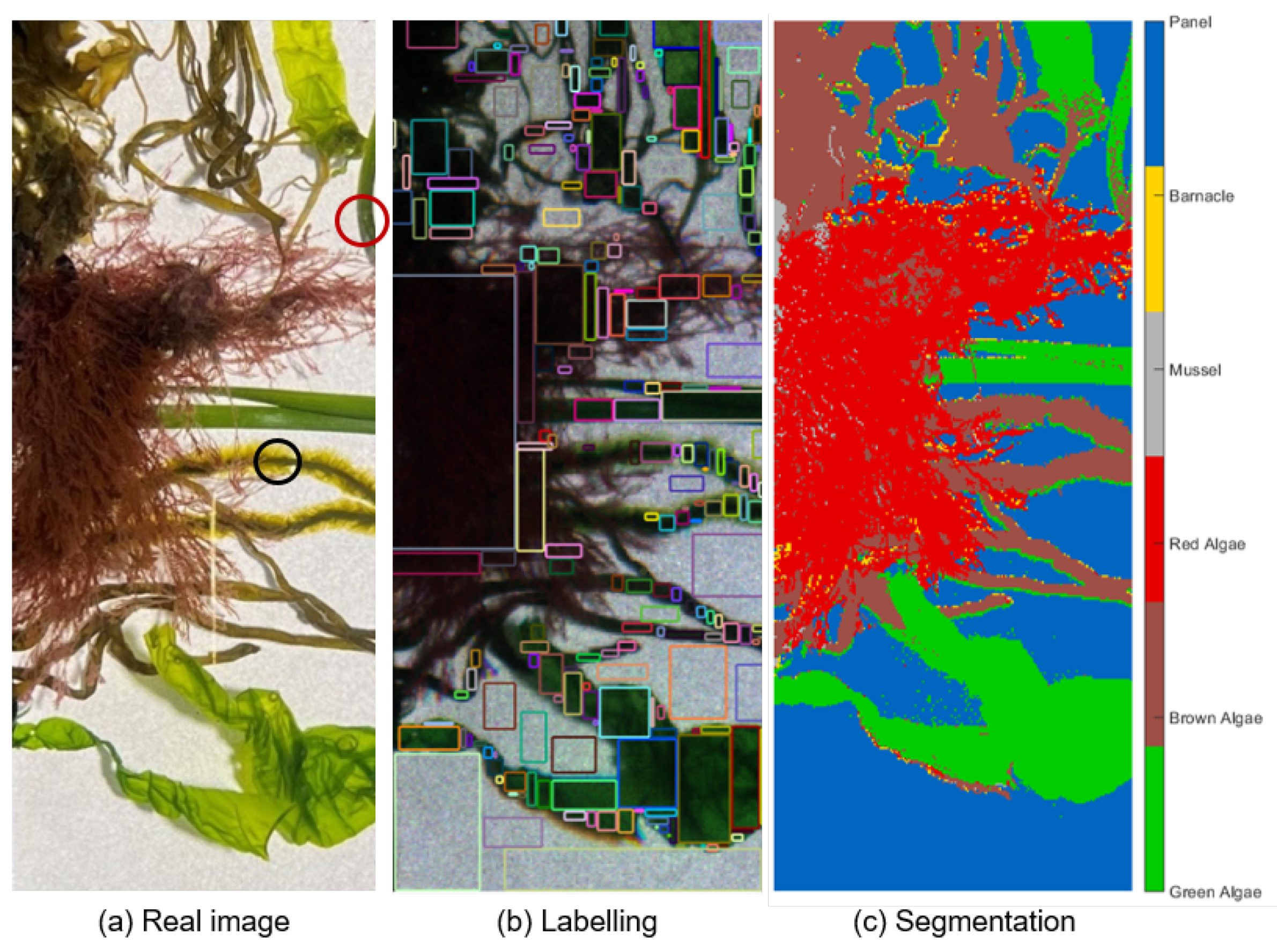
2.4.6. Evaluation of Real Fouled Panels
3. Results
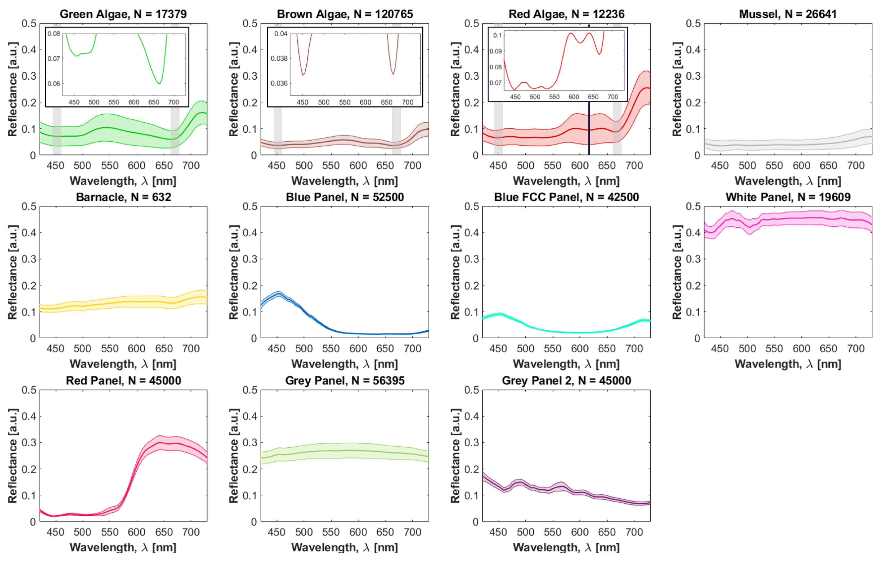
3.1. Spectral Library
3.2. Principal Component Analysis
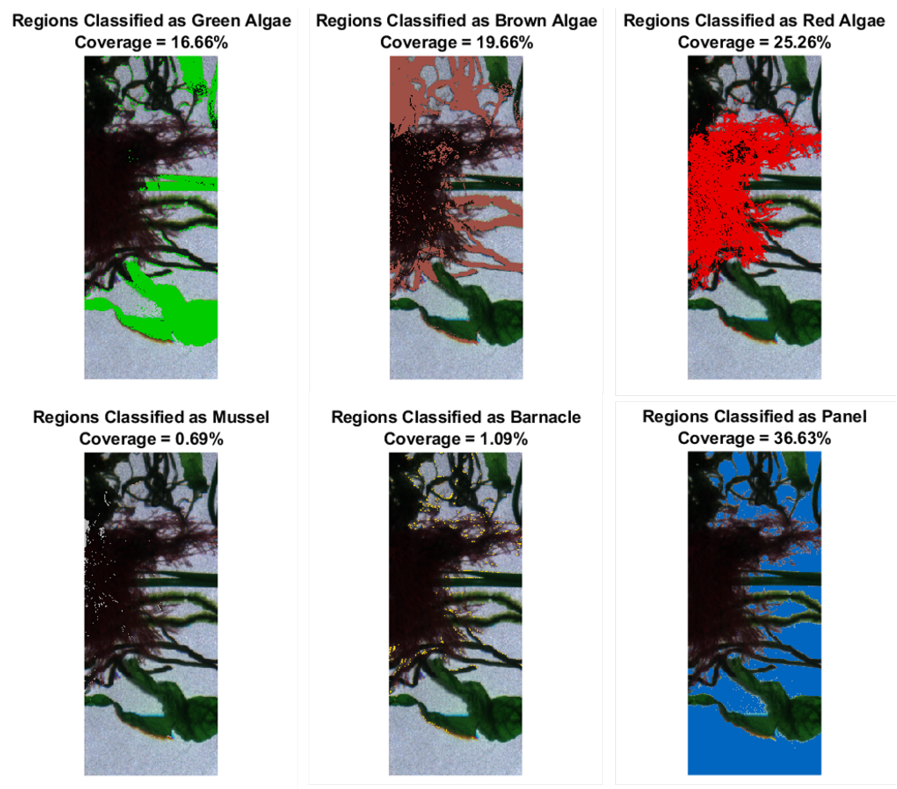
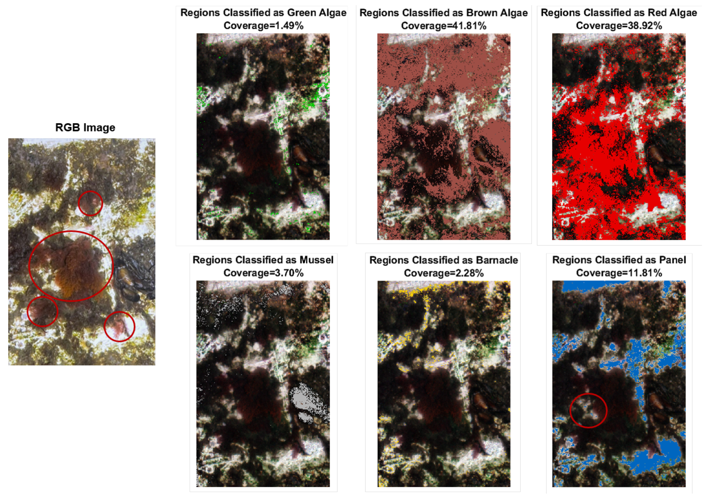
3.3. Classification and Coverage Estimation
3.3.1. Model Target
3.3.2. Fine Classification
3.3.3. Real Targets
4. Discussion and Conclusions
4.1. Staring-Type Hyperspectral Sensor
4.2. Spectral Library of Biofouling Species
4.3. Supervised Classification of Submerged Biofouled Panels
Supplementary Materials
Author Contributions
Funding
Institutional Review Board Statement
Informed Consent Statement
Data Availability Statement
Conflicts of Interest
Abbreviations
| ASTM | American Society for Testing and Materials |
| CA | clear aperture |
| CMTC | CoaST Maritime Test Centre |
| CWL | center wavelength |
| ECHA | European Chemicals Agency |
| EMCCD | electron multiplying charge-coupled device |
| FCC | fouling control coating |
| FDR | false discovery rate |
| FNR | false negative rate |
| FOV | field of view |
| FWHM | full-width at half-maximum |
| HSI | hyperspectral imaging |
| LCTF | liquid crystal tunable filter |
| LED | light-emitting diode |
| NA | numerical aperture |
| NIS | non-indigenous species |
| NSTM | naval ships’ technical manual |
| PC | principal component |
| PCA | principal component analysis |
| PPV | positive predictive value |
| ROI | region of interest |
| SNR | signal-to-noise ratio |
| SVM | support vector machine |
| TPR | true positive rate |
| WNN | wide neural network |
References
- Hopkins, G.A.; Forrest, B.M. A preliminary assessment of biofouling and non-indigenous marine species associated with commercial slow-moving vessels arriving in New Zealand. Biofouling 2010, 26, 613–621. [Google Scholar] [CrossRef] [PubMed]
- Ruiz, M.; Backer, H. HELCOM Guide to Alien Species and Ballast Water Management in the Baltic Sea; Technical Report; HELCOM—Baltic Marine Environment Protection Commission: Helsinki, Finland, 2014. [Google Scholar]
- Moser, C.S.; Wier, T.P.; First, M.R.; Grant, J.F.; Riley, S.C.; Robbins-Wamsley, S.H.; Tamburri, M.N.; Ruiz, G.M.; Miller, A.W.; Drake, L.A. Quantifying the extent of niche areas in the global fleet of commercial ships: The potential for “super-hot spots” of biofouling. Biol. Invasions 2017, 19, 1745–1759. [Google Scholar] [CrossRef]
- Jägerbrand, A.K.; Brutemark, A.; Barthel Svedén, J.; Gren, I.M. A review on the environmental impacts of shipping on aquatic and nearshore ecosystems. Sci. Total Environ. 2019, 695, 133637. [Google Scholar] [CrossRef] [PubMed]
- GloBallast. Global Ballast Water Management Programme. 2002. Available online: https://archive.iwlearn.net/globallast.imo.org/index.html (accessed on 10 February 2022).
- Yebra, D.M.; Kiil, S.; Dam-Johansen, K. Antifouling technology-Past, present and future steps towards efficient and environmentally friendly antifouling coatings. Prog. Org. Coat. 2004, 50, 75–104. [Google Scholar] [CrossRef]
- Schultz, M.P. Effects of coating roughness and biofouling on ship resistance and powering. Biofouling 2007, 23, 331–341. [Google Scholar] [CrossRef]
- Hellio, C.; Yebra, D. Advances in Marine Antifouling Coatings and Technologies; Woodhead Publishing: Cambridge, UK, 2009; p. 811. [Google Scholar]
- Callow, J.A.; Callow, M.E. Trends in the development of environmentally friendly fouling-resistant marine coatings. Nat. Commun. 2011, 2, 1–10. [Google Scholar] [CrossRef]
- Hu, P.; Xie, Q.; Ma, C.; Zhang, G. Silicone-Based Fouling-Release Coatings for Marine Antifouling. Langmuir 2020, 36, 2170–2183. [Google Scholar] [CrossRef]
- NSTM-NAVAL SHIPS’ TECHNICAL MANUAL. Waterborne Underwater Hull Cleaning of Navy Ships; Technical Report; Naval Sea Systems Command: Washington, NY, USA, 2006. [Google Scholar]
- ASTM D3623-78a; Standard Test Method for Testing Antifouling Panels in Shallow Submergence. Technical Report; ASTM International: West Conshohocken, PA, USA, 2012. [CrossRef]
- ECHA. Transitional Guidance on the Biocidal Products Regulation-Transitional Guidance on Efficacy Assessment for Product Type 21 Antifouling Products; Technical Report; European Chemicals Agency: Helsinki, Finland, 2014. [Google Scholar]
- Culverhouse, P.; Williams, R.; Reguera, B.; Herry, V.; González-Gil, S. Do experts make mistakes? A comparison of human and machine identification of dinoflagellates. Mar. Ecol. Prog. Ser. 2003, 247, 17–25. [Google Scholar] [CrossRef]
- Bloomfield, N.J.; Wei, S.; Woodham, A.B.; Wilkinson, P.; Robinson, A.P. Automating the assessment of biofouling in images using expert agreement as a gold standard. Sci. Rep. 2021, 11, 1–10. [Google Scholar] [CrossRef]
- Pedersen, M.L.; Weinell, C.E.; Ulusoy, B.; Dam-Johansen, K. Marine biofouling resistance rating using image analysis. J. Coat. Technol. Res. 2022, 19, 1127–1138. [Google Scholar] [CrossRef]
- MacLeod, N.; Benfield, M.; Culverhouse, P. Time to automate identification. Nature 2010, 467, 154–155. [Google Scholar] [CrossRef]
- Garg, S.; Singh, P. State-of-the-art review of deep learning for medical image analysis. In Proceedings of the 3rd International Conference on Intelligent Sustainable Systems, ICISS, Thoothukudi, India, 3–5 December 2020; pp. 421–427. [Google Scholar] [CrossRef]
- First, M.; Riley, S.; Islam, K.A.; Hill, V.; Li, J.; Zimmerman, R.; Drake, L. Rapid quantification of biofouling with an inexpensive, underwater camera and image analysis. Manag. Biol. Invasions 2021, 12, 599–617. [Google Scholar] [CrossRef]
- Chennu, A.; Färber, P.; De’ath, G.; De Beer, D.; Fabricius, K.E. A diver-operated hyperspectral imaging and topographic surveying system for automated mapping of benthic habitats. Sci. Rep. 2017, 7, 1–12. [Google Scholar] [CrossRef]
- Lu, G.; Fei, B. Medical hyperspectral imaging: A review. J. Biomed. Opt. 2014, 19, 010901. [Google Scholar] [CrossRef]
- Mogstad, A.A.; Johnsen, G.; Ludvigsen, M. Shallow-Water Habitat Mapping using Underwater Hyperspectral Imaging from an Unmanned Surface Vehicle: A Pilot Study. Remote Sens. 2019, 11, 685. [Google Scholar] [CrossRef]
- Hochberg, E.J.; Atkinson, M.J. Capabilities of remote sensors to classify coral, algae, and sand as pure and mixed spectra. Remote Sens. Environ. 2003, 85, 174–189. [Google Scholar] [CrossRef]
- Hedley, J.D.; Mumby, P.J. Biological and remote sensing perspectives of pigmentation in coral reef organisms. In Advances in Marine Biology; Elsevier Science: Amsterdam, The Netherlands, 2002; Volume 43, pp. 277–317. [Google Scholar] [CrossRef]
- Foglini, F.; Grande, V.; Marchese, F.; Bracchi, V.A.; Prampolini, M.; Angeletti, L.; Castellan, G.; Chimienti, G.; Hansen, I.M.; Gudmundsen, M.; et al. Application of hyperspectral imaging to underwater habitat mapping, Southern Adriatic Sea. Sensors 2019, 19, 2261. [Google Scholar] [CrossRef] [Green Version]
- Mogstad, A.A.; Johnsen, G. Spectral characteristics of coralline algae: A multi-instrumental approach, with emphasis on underwater hyperspectral imaging. Appl. Opt. 2017, 56, 9957–9975. [Google Scholar] [CrossRef]
- Duckey, T.; Lewis, M.; Chang, G. Optical oceanography: Recent advances and future directions using global remote sensing and in situ observations. Rev. Geophys. 2006, 44, 1–39. [Google Scholar] [CrossRef]
- Heumann, B.W. Satellite remote sensing of mangrove forests: Recent advances and future opportunities. Prog. Phys. Geogr. 2011, 35, 87–108. [Google Scholar] [CrossRef]
- Kazemipour, F.; Launeau, P.; Méléder, V. Microphytobenthos biomass mapping using the optical model of diatom biofilms: Application to hyperspectral images of Bourgneuf Bay. Remote Sens. Environ. 2012, 127, 1–13. [Google Scholar] [CrossRef]
- Chennu, A.; Färber, P.; Volkenborn, N.; Al-Najjar, M.A.; Janssen, F.; de Beer, D.; Polerecky, L. Hyperspectral imaging of the microscale distribution and dynamics of microphytobenthos in intertidal sediments. Limnol. Oceanogr. Methods 2013, 11, 511–528. [Google Scholar] [CrossRef]
- Johnsen, G. Underwater Hyperspectral Imaging. U.S. Patent 8502974 B2, 6 August 2013. [Google Scholar]
- Johnsen, G.; Volent, Z.; Dierssen, H.; Pettersen, R.; Ardelan, M.; Søreide, F.; Fearns, P.; Ludvigsen, M.; Moline, M. Underwater hyperspectral imagery to create biogeochemical maps of seafloor properties. In Subsea Optics and Imaging; Elsevier: Amsterdam, The Netherlands, 2013; pp. 508–540. [Google Scholar] [CrossRef]
- Dumke, I.; Nornes, S.M.; Purser, A.; Marcon, Y.; Ludvigsen, M.; Ellefmo, S.L.; Johnsen, G.; Søreide, F. First hyperspectral imaging survey of the deep seafloor: High-resolution mapping of manganese nodules. Remote Sens. Environ. 2018, 209, 19–30. [Google Scholar] [CrossRef]
- Pope, R.M.; Fry, E.S. Absorption spectrum (380–700 nm) of pure water II Integrating cavity measurements. Appl. Opt. 1997, 36, 8710–8723. [Google Scholar] [CrossRef]
- Liu, B.; Liu, Z.; Men, S.; Li, Y.; Ding, Z.; He, J.; Zhao, Z. Underwater Hyperspectral Imaging Technology and Its Applications for Detecting and Mapping the Seafloor: A Review. Sensors 2020, 20, 4962. [Google Scholar] [CrossRef]
- Burger, J.; Geladi, P. Hyperspectral NIR image regression part I: Calibration and correction. J. Chemom. 2006, 19, 355–363. [Google Scholar] [CrossRef]
- Nutrients and Eutrophication in Danish Marine Waters-Hydrography. Available online: https://www2.dmu.dk/1_viden/2_miljoe-tilstand/3_vand/4_eutrophication/hydrography.asp (accessed on 4 February 2022).
- CEPE Antifouling Working Group. Efficacy Evaluation of Antifouling Products. Conduct and Reporting of Static Raft Tests for Antifouling Efficacy; Technical Report; The European Council of Producers and Importers of Paints, Printing Inks and Artists’ Colors (CEPE): Brussels, Belgium, 2012. [Google Scholar]
- Larsen, J.G.; Hansen, P.J. Tang; Naturhistorisk Museum: Copenhagen, Denmark, 2020. [Google Scholar]
- Huot, M.; Dalgleish, F.; Rehm, E.; Pich, M.; Archambault, P. Underwater Multispectral Laser Serial Imager for Spectral Differentiation of Macroalgal and Coral Substrates. Remote Sens. 2022, 14, 3105. [Google Scholar] [CrossRef]
- Gat, N. Imaging spectroscopy using tunable filters: A review. Wavelet Appl. VII 2000, 4056, 50–64. [Google Scholar] [CrossRef]
- Cassarly, W.J. Recent advances in mixing rods. Illum. Opt. 2008, 7103, 710307. [Google Scholar] [CrossRef]
- Moreno, I. Output irradiance of tapered lightpipes. J. Opt. Soc. Am. A 2010, 27, 1985. [Google Scholar] [CrossRef] [PubMed]
- Song, H.; Mehdi, S.R.; Wu, C.; Li, Z.; Gong, H.; Ali, A.; Huang, H. Underwater spectral imaging system based on liquid crystal tunable filter. J. Mar. Sci. Eng. 2021, 9, 1206. [Google Scholar] [CrossRef]
- Shaikh, M.S.; Jaferzadeh, K.; Thörnberg, B.; Casselgren, J. Calibration of a hyper-spectral imaging system using a low-cost reference. Sensors 2021, 21, 3738. [Google Scholar] [CrossRef]
- Liu, H.; Sticklus, J.; Köser, K.; Hoving, H.J.T.; Song, H.; Chen, Y.; Greinert, J.; Schoening, T. TuLUMIS-A tunable LED-based underwater multispectral imaging system. Opt. Express 2018, 26, 7811. [Google Scholar] [CrossRef]
- Ødegård, Ø.; Mogstad, A.A.; Johnsen, G.; Sørensen, A.J.; Ludvigsen, M. Underwater hyperspectral imaging: A new tool for marine archaeology. Appl. Opt. 2018, 57, 3214. [Google Scholar] [CrossRef]
- Amigo, J.M.; Babamoradi, H.; Elcoroaristizabal, S. Hyperspectral image analysis-A tutorial. Anal. Chim. Acta 2015, 896, 34–51. [Google Scholar] [CrossRef]
- Cimoli, E.; Meiners, K.M.; Lucieer, A.; Lucieer, V. An under-ice hyperspectral and RGB imaging system to capture fine-scale biophysical properties of sea ice. Remote Sens. 2019, 11, 2860. [Google Scholar] [CrossRef] [Green Version]
- Shlens, J. A Tutorial on Principal Component Analysis. arXiv 2014, arXiv:1404.1100. [Google Scholar] [CrossRef]
- Rodarmel, C.; Shan, J. Principal component analysis for hyperspectral image classification. Surv. Land Inf. Sci. 2002, 62, 115–122. [Google Scholar]
- Chen, Y.; Jiang, H.; Li, C.; Jia, X.; Ghamisi, P. Deep Feature Extraction and Classification of Hyperspectral Images Based on Convolutional Neural Networks. IEEE Trans. Geosci. Remote Sens. 2016, 54, 6232–6251. [Google Scholar] [CrossRef]
- Raczko, E.; Zagajewski, B. Comparison of support vector machine, random forest and neural network classifiers for tree species classification on airborne hyperspectral APEX images. Eur. J. Remote Sens. 2017, 50, 144–154. [Google Scholar] [CrossRef]
- Mathworks Inc. Statistics and Machine Learning Toolbox-MATLAB. Available online: https://se.mathworks.com/products/statistics.html (accessed on 6 July 2022).
- Paoletti, M.E.; Haut, J.M.; Plaza, J.; Plaza, A. ISPRS Journal of Photogrammetry and Remote Sensing Deep learning classifiers for hyperspectral imaging: A review. ISPRS J. Photogramm. Remote Sens. 2019, 158, 279–317. [Google Scholar] [CrossRef]
- Pettersen, R.; Johnsen, G.; Bruheim, P.; Andreassen, T. Development of hyperspectral imaging as a bio-optical taxonomic tool for pigmented marine organisms. Org. Divers. Evol. 2014, 14, 237–246. [Google Scholar] [CrossRef]
- Smith, C.M.; Alberte, R.S. Characterization of in vivo absorption features of chlorophyte, phaeophyte and rhodophyte algal species. Mar. Biol. 1994, 118, 511–521. [Google Scholar] [CrossRef]
- Nielsen, J.H.; Pedersen, C.; Kiørboe, T.; Nikolajsen, T.; Brydegaard, M.; Rodrigo, P.J. Investigation of autofluorescence in zooplankton for use in classification of larval salmon lice. Appl. Opt. 2019, 58, 7022–7027. [Google Scholar] [CrossRef] [PubMed]
- Olmedo-Masat, O.M.; Paula Raffo, M.; Rodríguez-Pérez, D.; Arijón, M.; Sánchez-Carnero, N. How far can we classify macroalgae remotely? An example using a new spectral library of species from the south west atlantic (argentine patagonia). Remote Sens. 2020, 12, 3870. [Google Scholar] [CrossRef]
- Grill, C. Analysing spectral data: Comparison and application of two techniques. Biol. J. Linn. Soc. 2000, 69, 121–138. [Google Scholar] [CrossRef]
- Zhao, G.; Ljungholm, M.; Malmqvist, E.; Bianco, G.; Hansson, L.A.; Svanberg, S.; Brydegaard, M. Inelastic hyperspectral lidar for profiling aquatic ecosystems. Laser Photonics Rev. 2016, 10, 807–813. [Google Scholar] [CrossRef]
- Menchaca, I.; Zorita, I.; Rodríguez-Espeleta, N.; Erauskin, E.; Erauskin, C.; Liria, P.; Santesteban, M.; Mendibil, I.; Urtizberea, I. Guide for the evaluation of biofouling formation in the marine environment. Rev. De Investig. Mar. 2014, 21, 90–99. [Google Scholar]
- Hu, W.; Huang, Y.; Wei, L.; Zhang, F.; Li, H. Deep convolutional neural networks for hyperspectral image classification. J. Sens. 2015, 2015, 258619. [Google Scholar] [CrossRef] [Green Version]


Publisher’s Note: MDPI stays neutral with regard to jurisdictional claims in published maps and institutional affiliations. |
© 2022 by the authors. Licensee MDPI, Basel, Switzerland. This article is an open access article distributed under the terms and conditions of the Creative Commons Attribution (CC BY) license (https://creativecommons.org/licenses/by/4.0/).
Share and Cite
Santos, J.; Pedersen, M.L.; Ulusoy, B.; Weinell, C.E.; Pedersen, H.C.; Petersen, P.M.; Dam-Johansen, K.; Pedersen, C. A Tunable Hyperspectral Imager for Detection and Quantification of Marine Biofouling on Coated Surfaces. Sensors 2022, 22, 7074. https://doi.org/10.3390/s22187074
Santos J, Pedersen ML, Ulusoy B, Weinell CE, Pedersen HC, Petersen PM, Dam-Johansen K, Pedersen C. A Tunable Hyperspectral Imager for Detection and Quantification of Marine Biofouling on Coated Surfaces. Sensors. 2022; 22(18):7074. https://doi.org/10.3390/s22187074
Chicago/Turabian StyleSantos, Joaquim, Morten Lysdahlgaard Pedersen, Burak Ulusoy, Claus Erik Weinell, Henrik Chresten Pedersen, Paul Michael Petersen, Kim Dam-Johansen, and Christian Pedersen. 2022. "A Tunable Hyperspectral Imager for Detection and Quantification of Marine Biofouling on Coated Surfaces" Sensors 22, no. 18: 7074. https://doi.org/10.3390/s22187074