
Estimation of Soil Organic Carbon Using Vis-NIR Spectral Data and Spectral Feature Bands Selection in Southern Xinjiang, China


Abstract
:1. Introduction
2. Materials and Methods
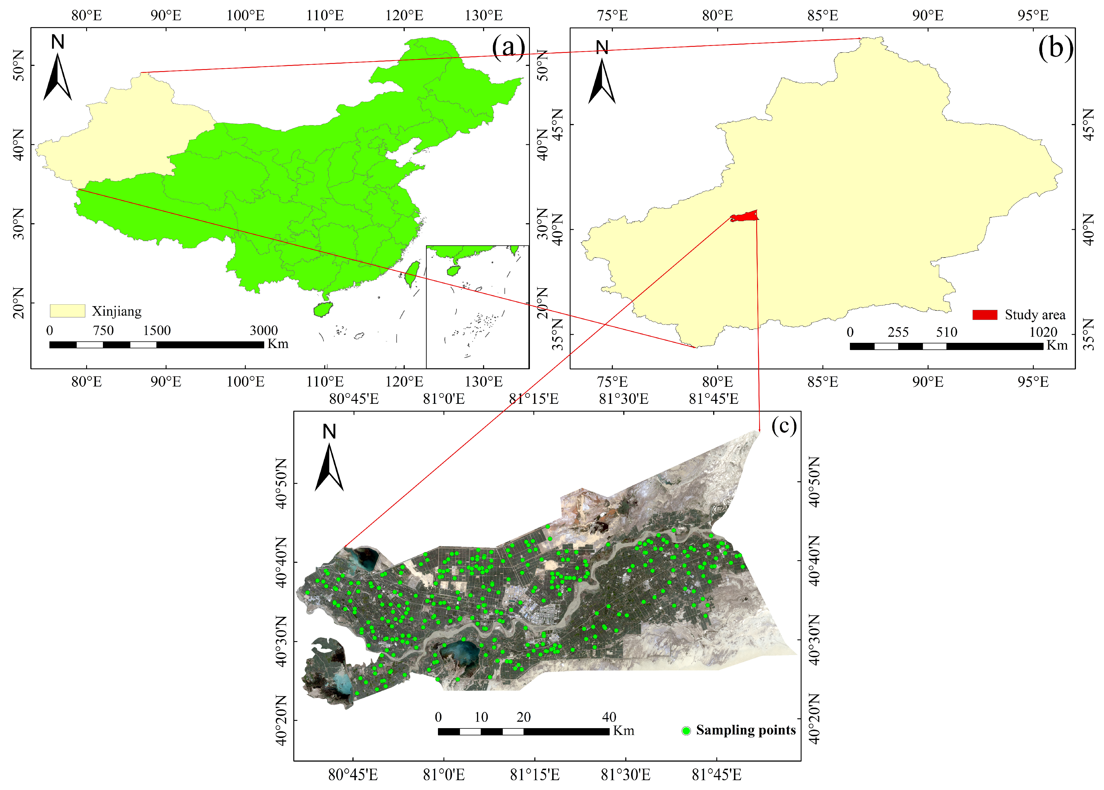
2.1. Study Area
2.2. Soil Sampling and Laboratory Analysis
2.3. Soil Spectra Collection and Pre-Processing
2.4. Sample Selection Algorithm
2.5. Spectral Feature Bands Selection Algorithm
2.6. Modeling Development
2.6.1. PLSR
2.6.2. RF
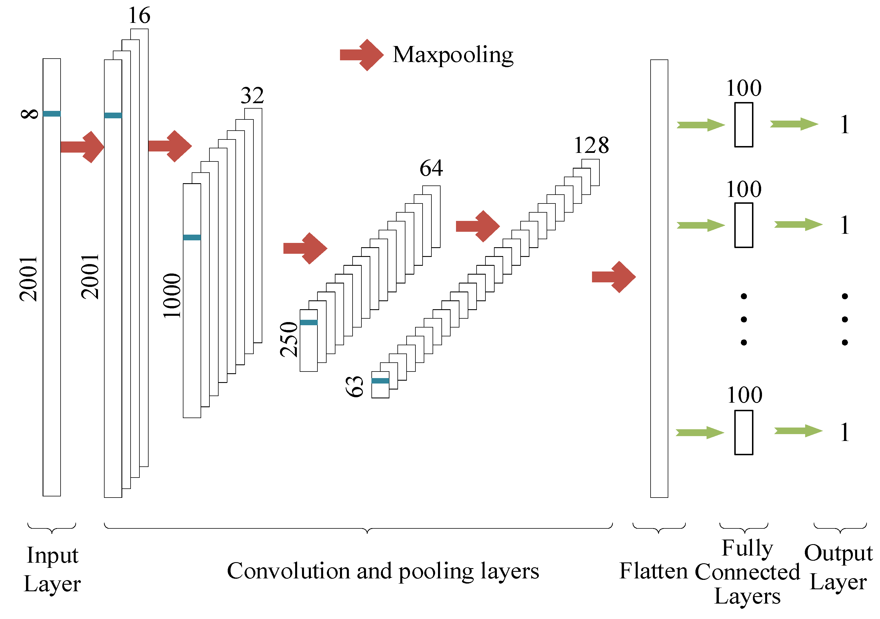
2.6.3. CNN
2.7. Indicators for Model Evaluation
3. Results
3.1. Descriptive Statistics of SOC
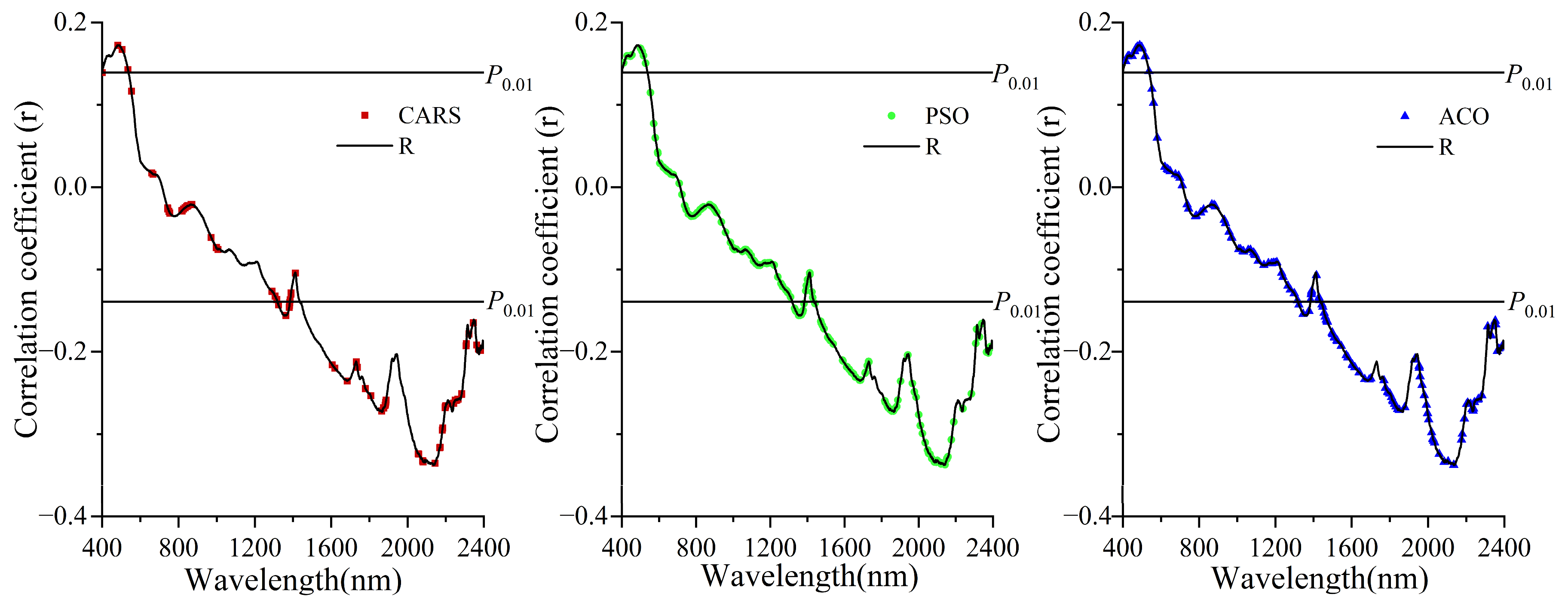
3.2. Feature Band Selection Based on CARS, PSO and ACO
3.3. Correlation Analysis between SOC and Spectrum
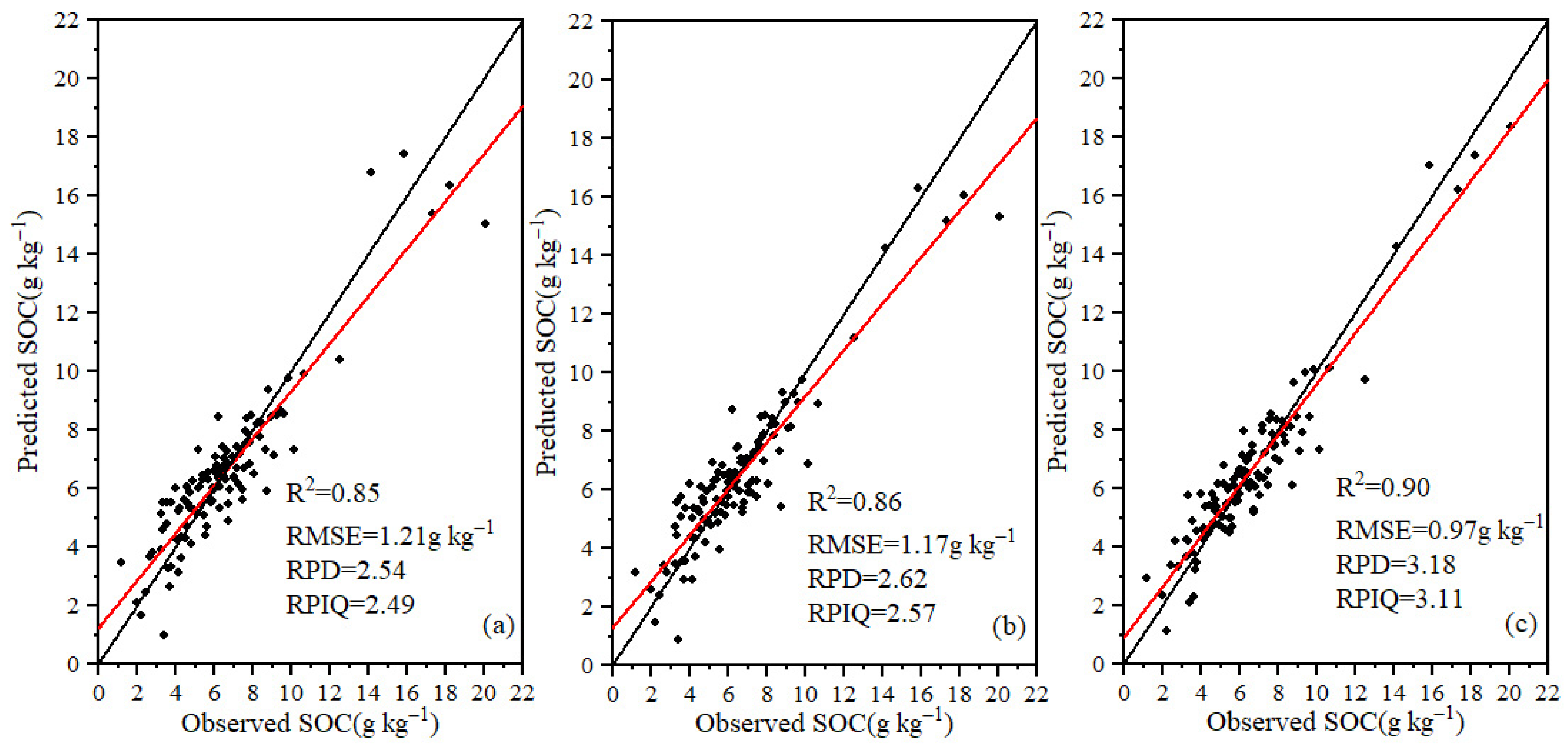
3.4. SOC Estimation Models Performance
4. Discussion
4.1. Effects of Feature Band Selection Algorithm on Model Performance
4.2. Performance Comparison of CNN and Traditional Prediction Models
5. Conclusions
Author Contributions
Funding
Institutional Review Board Statement
Informed Consent Statement
Data Availability Statement
Conflicts of Interest
References
- Hu, B.; Xie, M.; Li, H.; Zhao, W.; Hu, J.; Jiang, Y.; Ji, W.; Li, S.; Hong, Y.; Yang, M.; et al. Stoi-chiometry of soil carbon, nitrogen, and phosphorus in farmland soils in Southern China: Spatial pattern and related domi-nates. Catena 2022, 217, 106468. [Google Scholar] [CrossRef]
- Bellon-Maurel, V.; McBratney, A. Near-infrared (NIR) and mid-infrared (MIR) spectroscopic techniques for assessing the amount of carbon stock in soils-Critical review and research perspectives. Soil Biol. Biochem. 2011, 43, 1398–1410. [Google Scholar] [CrossRef]
- Chen, S.; Xu, D.; Li, S.; Ji, W.; Yang, M.; Zhou, Y.; Hu, B.; Xu, H.; Shi, Z. Monitoring soil organic carbon in alpine soils using in situ vis-NIR spectroscopy and a multilayer perceptron. Land Degrad. Dev. 2020, 31, 1026–1038. [Google Scholar] [CrossRef]
- Gu, X.; Wang, Y.; Sun, Q.; Yang, G.; Zhang, C. Hyperspectral inversion of soil organic matter content in cultivated land based on wavelet transform. Comput. Electron. Agric. 2019, 167, 105053. [Google Scholar] [CrossRef]
- Gruszczyński, S.; Gruszczyński, W. Supporting soil and land assessment with machine learning models using the Vis-NIR spectral response. Geoderma 2022, 405, 115451. [Google Scholar] [CrossRef]
- Gomez, C.; Chevallier, T.; Moulin, P.; Bouferra, I.; Hmaidi, K.; Arrouays, D.; Barthès, B.G. Prediction of soil organic and inorganic carbon concentrations in Tunisian samples by mid-infrared reflectance spectroscopy using a French national library. Geoderma 2020, 375, 114469. [Google Scholar] [CrossRef]
- Stoner, E.R.; Baumgardner, M.F. Characteristic variations in reflectance of surface soils. Soil Sci. Soc. Am. J. 1981, 45, 1161–1165. [Google Scholar] [CrossRef]
- Li, H.; Liang, Y.; Xu, Q.; Cao, D. Key wavelengths screening using competitive adaptive reweighted sampling method for multivariate calibration. Anal. Chim. Acta 2009, 648, 77–84. [Google Scholar] [CrossRef]
- Sun, W.; Zhang, X. Estimating soil zinc concentrations using reflectance spectroscopy. Int. J. Appl. Earth Obs. Geoinf. 2017, 58, 126–133. [Google Scholar] [CrossRef]
- Bao, Y.; Meng, X.; Ustin, S.; Wang, X.; Zhang, X.; Liu, H.; Tang, H. Vis-SWIR spectral prediction model for soil organic matter with different grouping strategies. Catena 2020, 195, 104703. [Google Scholar] [CrossRef]
- Bao, Y.; Meng, X.; Ustin, S.; Wang, X.; Zhang, X.; Liu, H.; Tang, H. Estimation of soil organic matter content based on CARS algorithm coupled with random forest. Spectrochim. Acta Part. A Mol. Biomol. Spectrosc. 2021, 258, 119823. [Google Scholar]
- Sun, W.; Liu, S.; Zhang, X.; Li, Y. Estimation of soil organic matter content using selected spectral subset of hyperspectral data. Geoderma 2022, 409, 115653. [Google Scholar] [CrossRef]
- Rossel, R.A.V.; Behrens, T. Using data mining to model and interpret soil diffuse reflectance spectra. Geoderma 2010, 158, 46–54. [Google Scholar] [CrossRef]
- Yan, F.; Shangguan, W.; Zhang, J.; Hu, B. Depth-to-bedrock map of China at a spatial resolution of 100 meters. Sci. Data 2020, 7, 1–13. [Google Scholar] [CrossRef]
- Berger, K.; Verrelst, J.; Feret, J.B.; Wang, Z.; Wocher, M.; Strathmann, M.; Hank, T. Crop nitrogen monitoring: Recent progress and principal developments in the context of imaging spectroscopy missions. Remote Sens. Environ. 2020, 242, 111758. [Google Scholar] [CrossRef]
- LeCun, Y.; Bengio, Y.; Hinton, G. Deep learning. Nature 2015, 521, 436–444. [Google Scholar] [CrossRef] [PubMed]
- Veres, M.; Lacey, G.; Taylor, G.W. Deep learning architectures for soil property prediction. In Proceedings of the 2015 12th Conference on Computer and Robot Vision, Halifax, NS, Canada, 3–5 June 2015; pp. 8–15. [Google Scholar]
- Liu, L.; Ji, M.; Buchroithner, M. Transfer learning for soil spectroscopy based on convolutional neural networks and its application in soil clay content mapping using hyperspectral imagery. Sensors 2018, 18, 3169. [Google Scholar] [CrossRef]
- Padarian, J.; Minasny, B.; McBratney, A.B. Transfer learning to localise a continental soil vis-NIR calibration model. Geoderma 2019, 340, 279–288. [Google Scholar] [CrossRef]
- Peng, J.; Biswas, A.; Jiang, Q.; Zhao, R.; Hu, B.; Shi, Z. Estimating soil salinity from remote sensing and terrain data in Southern Xinjiang province, China. Geoderma 2019, 337, 1309–1319. [Google Scholar] [CrossRef]
- Hu, B.; Chen, S.; Hu, J.; Xia, F.; Xu, J.; Li, Y.; Shi, Z. Application of portable XRF and VNIR sensors for rapid assessment of soil heavy metal pollution. PLoS ONE 2017, 12, e0172438. [Google Scholar] [CrossRef]
- Galvao, R.K.H.; Araujo, M.C.U.; José, G.E.; Pontes, M.J.C.; Silva, E.C.; Saldanha, T.C.B. A method for calibration and validation subset partitioning. Talanta 2015, 67, 736–740. [Google Scholar] [CrossRef] [PubMed]
- Farrés, M.; Platikanov, S.; Tsakovski, S.; Tauler, R. Comparison of the variable importance in projection (VIP) and of the selectivity ratio (SR) methods for variable selection and interpretation. J. Chemom. 2015, 29, 528–536. [Google Scholar] [CrossRef]
- Jin, X.; Du, J.; Liu, H.; Wang, Z.; Song, K. Remote estimation of soil organic matter content in the Sanjiang Plain, Northest China: The optimal band algorithm versus the GRA-ANN model. Agric. For. Meteorol. 2016, 218, 250–260. [Google Scholar] [CrossRef]
- Meng, X.; Bao, Y.; Liu, J.; Liu, H.; Zhang, X.; Zhang, Y.; Kong, F. Regional soil organic carbon prediction model based on a discrete wavelet analysis of hyperspectral satellite data. Int. J. Appl. Earth Obs. Geoinf. 2020, 89, 102111. [Google Scholar] [CrossRef]
- Zhang, Z.; Ding, J.; Zhu, C.; Wang, J. Combination of efficient signal pre-processing and optimal band combination algorithm to predict soil organic matter through visible and near-infrared spectra. Spectrochim. Acta Part. A Mol. Biomol. Spectrosc. 2020, 240, 118553. [Google Scholar] [CrossRef]
- Xu, S.; Wang, M.; Shi, X. Hyperspectral imaging for high-resolution mapping of soil carbon fractions in intact paddy soil profiles with multivariate techniques and variable selection. Geoderma 2020, 370, 114358. [Google Scholar] [CrossRef]
- Fan, A.; Xu, T.; Teng, G.; Wang, X.; Zhang, Y.; Pan, C. Hyperspectral polarization-compressed imaging and reconstruction with sparse basis optimized by particle swarm optimization. Chemom. Intell. Lab. Syst. 2020, 206, 104163. [Google Scholar] [CrossRef]
- Dorigo, M.; Gambardella, L.M. Ant colony system: A cooperative learning approach to the traveling salesman problem. IEEE Trans. Evol. Comput. 1997, 1, 53–66. [Google Scholar] [CrossRef]
- Hu, B.; Bourennane, H.; Arrouays, D.; Denoroy, P.; Lemercier, B.; Saby, N.P. Developing pedotransfer functions to harmonize extractable soil phosphorus content measured with different methods: A case study across the mainland of France. Geoderma 2021, 381, 114645. [Google Scholar] [CrossRef]
- Hong, Y.; Chen, S.; Liu, Y.; Zhang, Y.; Yu, L.; Chen, Y.; Liu, Y. Combination of fractional order derivative and memory-based learning algorithm to improve the estimation accuracy of soil organic matter by visible and near-infrared spectroscopy. Catena 2019, 174, 104–116. [Google Scholar] [CrossRef]
- Hutengs, C.; Seidel, M.; Oertel, F.; Ludwig, B.; Vohland, M. In situ and laboratory soil spectroscopy with portable visible-to-near-infrared and mid-infrared instruments for the assessment of organic carbon in soils. Geoderma 2019, 355, 113900. [Google Scholar] [CrossRef]
- Hu, B.; Xue, J.; Zhou, Y.; Shao, S.; Fu, Z.; Li, Y.; Shi, Z. Modelling bioaccumulation of heavy metals in soil-crop ecosystems and identifying its controlling factors using machine learning. Environ. Pollut. 2020, 262, 114308. [Google Scholar] [CrossRef] [PubMed]
- Andrade, R.; Faria, W.M.; Silva, S.H.G.; Chakraborty, S.; Weindorf, D.C.; Mesquita, L.F.; Curi, N. Prediction of soil fertility via portable X-ray fluorescence (pXRF) spectrometry and soil texture in the Brazilian Coastal Plains. Geoderma 2020, 357, 113960. [Google Scholar] [CrossRef]
- Hu, B.; Zhou, Q.; He, C.; Duan, L.; Li, W.Y.; Zhang, G.; Ji, W.; Peng, J.; Xie, H.X. Spatial variability and potential controls of soil organic matter in the Eastern Dongting Lake Plain in southern China. J. Soils Sediments 2021, 21, 2791–2804. [Google Scholar] [CrossRef]
- Zhu, C.; Ding, J.; Zhang, Z.; Wang, Z. Exploring the potential of UAV hyperspectral image for estimating soil salinity: Effects of optimal band combination algorithm and random forest. Spectrochim. Acta Part. A Mol. Biomol. Spectrosc. 2022, 279, 121416. [Google Scholar] [CrossRef]
- Ng, W.; Minasny, B.; Montazerolghaem, M.; Padarian, J.; Ferguson, R.; Bailey, S.; McBratney, A.B. Convolutional neural network for simultaneous prediction of several soil properties using visible/near-infrared, mid-infrared, and their combined spectra. Geoderma 2019, 352, 251–267. [Google Scholar] [CrossRef]
- Cui, C.; Fearn, T. Modern practical convolutional neural networks for multivariate regression: Applications to NIR calibration. Chemom. Intell. Lab. Syst. 2018, 182, 9–20. [Google Scholar] [CrossRef]
- Bergstra, J.; Yamins, D.; Cox, D. Making a science of model search: Hyperparameter optimization in hundreds of dimensions for vision architectures. Int. Conf. Mach. Learn. 2013, 28, 115–123. [Google Scholar]
- Chang, C.W.; Laird, D.A.; Mausbach, M.J.; Hurburgh, C.R. Near-infrared reflectance spectroscopy–principal components regression analyses of soil properties. Soil Sci. Soc. Am. J. 2001, 65, 480–490. [Google Scholar] [CrossRef]
- Wijewardane, N.K.; Ge, Y.; Morgan, C.L.S. Moisture insensitive prediction of soil properties from VNIR reflectance spectra based on external parameter orthogonalization. Geoderma 2016, 267, 92–101. [Google Scholar] [CrossRef]
- Kuang, B.; Mouazen, A.M. Calibration of visible and near infrared spectroscopy for soil analysis at the field scale on three European farms. Eur. J. Soil Sci. 2011, 62, 629–636. [Google Scholar] [CrossRef]
- Prasad, B.; Sinha, M.K. Properties of poultry litter humic acid fractions and their metal-complexes. Plant. Soil 1981, 63, 439–448. [Google Scholar] [CrossRef]
- Padermshoke, A.; Sato, H.; Katsumoto, Y.; Ekgasit, S.; Noda, I.; Ozaki, Y. Thermally induced phase transition of poly (3-hydroxybutyrate-co-3-hydroxyhexanoate) investigated by two-dimensional infrared correlation spectroscopy. Vib. Spectrosc. 2004, 36, 241–249. [Google Scholar] [CrossRef]
- Wang, J.; Ding, J.; Yu, D.; Ma, X.; Zhang, Z.; Ge, X.; Guo, Y. Capability of Sentinel-2 MSI data for monitoring and mapping of soil salinity in dry and wet seasons in the Ebinur Lake region, Xinjiang, China. Geoderma 2019, 353, 172–187. [Google Scholar] [CrossRef]
- Yang, X.; Song, J.; Peng, L.; Gao, L.; Liu, X.; Xie, L.; Li, G. Improving identification ability of adulterants in powdered Panax notoginseng using particle swarm optimization and data fusion. Infrared Phys. Technol. 2019, 103, 103101. [Google Scholar] [CrossRef]
- Zhang, Y.; Li, M.; Zheng, L.; Qin, Q.; Lee, W.S. Spectral features extraction for estimation of soil total nitrogen content based on modified ant colony optimization algorithm. Geoderma 2019, 333, 23–34. [Google Scholar] [CrossRef]
- Xing, Z.; Du, C.; Shen, Y.; Ma, F.; Zhou, J. A method combining FTIR-ATR and Raman spectroscopy to determine soil organic matter: Improvement of prediction accuracy using competitive adaptive reweighted sampling (CARS). Comput. Electron. Agric. 2021, 191, 106549. [Google Scholar] [CrossRef]
- Van Waes, C.; Mestdagh, I.; Lootens, P.; Carlier, L. Possibilities of near infrared reflectance spectroscopy for the prediction of organic carbon concentrations in grassland soils. J. Agric. Sci. 2005, 143, 487–492. [Google Scholar] [CrossRef]
- Xu, L.H.; Xie, D.T.; Wei, C.F.; Li, B. Prediction of total nitrogen and total phosphorus concentrations in purple soil using hyperspectral data. Spectrosc. Spectr. Anal. 2013, 33, 723–727. [Google Scholar]
- Zhang, J.J.; Tian, Y.C.; Yao, X.; Cao, W.X.; Ma, X.M.; Zhu, Y. Estimating soil total nitrogen content based on hyperspectral analysis technology. J. Nat. Resour. 2011, 26, 881–890. [Google Scholar]
- Dalal, R.C.; Henry, R.J. Simultaneous determination of moisture, organic carbon, and total nitrogen by near infrared reflectance spectrophotometry. Soil Sci. Soc. Am. J. 1986, 50, 120–123. [Google Scholar] [CrossRef]
- Breiman, L. Random forests. Mach. Learn. 2001, 45, 5–32. [Google Scholar] [CrossRef]
- Petralia, F.; Wang, P.; Yang, J.; Tu, Z. Integrative random forest for gene regulatory network inference. Bioinformatics 2015, 31, i197–i205. [Google Scholar] [CrossRef] [PubMed]
- Ma, L.; Liu, Y.; Zhang, X.; Ye, Y.; Yin, G.; Johnson, B.A. Deep learning in remote sensing applications: A meta-analysis and review. ISPRS J. Photogramm. Remote Sens. 2019, 152, 166–177. [Google Scholar] [CrossRef]
- Yuan, Q.; Shen, H.; Li, T.; Li, Z.; Li, S.; Jiang, Y.; Zhang, L. Deep learning in environmental remote sensing: Achievements and challenges. Remote Sens. Environ. 2020, 241, 111716. [Google Scholar] [CrossRef]
- Somarathna, P.; Minasny, B.; Malone, B.P. More data or a better model? Figuring out what matters most for the spatial prediction of soil carbon. Soil Sci. Soc. Am. J. 2017, 81, 1413–1426. [Google Scholar] [CrossRef]


| Sample Set | Number | Range | Mean | SD | CV (%) | Kurtosis | Skewness |
|---|---|---|---|---|---|---|---|
| Calibration | 220 | 0.98~20.49 | 6.54 | 3.08 | 47.12 | 5.54 | 1.92 |
| Validation | 110 | 1.19~20.04 | 6.54 | 3.09 | 47.19 | 5.53 | 1.91 |
| Entire | 330 | 0.98~20.49 | 6.54 | 3.08 | 47.14 | 5.43 | 1.91 |
| Dataset | Model | Calibration | Validation | ||||
|---|---|---|---|---|---|---|---|
| R2 | RMSE (g kg−1) | R2 | RMSE (g kg−1) | RPD | RPIQ | ||
| PLSR | 0.84 | 1.21 | 0.80 | 1.33 | 2.23 | 1.90 | |
| Full-band | RF | 0.83 | 1.26 | 0.80 | 1.32 | 2.25 | 1.96 |
| CNN | 0.84 | 1.20 | 0.81 | 1.31 | 2.27 | 2.02 | |
| PLSR | 0.90 | 0.98 | 0.85 | 1.21 | 2.54 | 2.49 | |
| CARS | RF | 0.93 | 0.87 | 0.86 | 1.17 | 2.62 | 2.57 |
| CNN | 0.94 | 0.72 | 0.90 | 0.97 | 3.18 | 3.11 | |
| PLSR | 0.85 | 1.20 | 0.82 | 1.29 | 2.32 | 2.15 | |
| PSO | RF | 0.87 | 1.15 | 0.84 | 1.24 | 2.45 | 2.26 |
| CNN | 0.87 | 1.16 | 0.85 | 1.22 | 2.53 | 2.36 | |
| PLSR | 0.86 | 1.14 | 0.83 | 1.27 | 2.39 | 2.19 | |
| ACO | RF | 0.87 | 1.15 | 0.84 | 1.26 | 2.42 | 2.28 |
| CNN | 0.88 | 1.09 | 0.86 | 1.17 | 2.57 | 2.53 | |
Publisher’s Note: MDPI stays neutral with regard to jurisdictional claims in published maps and institutional affiliations. |
© 2022 by the authors. Licensee MDPI, Basel, Switzerland. This article is an open access article distributed under the terms and conditions of the Creative Commons Attribution (CC BY) license (https://creativecommons.org/licenses/by/4.0/).
Share and Cite
Bai, Z.; Xie, M.; Hu, B.; Luo, D.; Wan, C.; Peng, J.; Shi, Z. Estimation of Soil Organic Carbon Using Vis-NIR Spectral Data and Spectral Feature Bands Selection in Southern Xinjiang, China. Sensors 2022, 22, 6124. https://doi.org/10.3390/s22166124
Bai Z, Xie M, Hu B, Luo D, Wan C, Peng J, Shi Z. Estimation of Soil Organic Carbon Using Vis-NIR Spectral Data and Spectral Feature Bands Selection in Southern Xinjiang, China. Sensors. 2022; 22(16):6124. https://doi.org/10.3390/s22166124
Chicago/Turabian StyleBai, Zijin, Modong Xie, Bifeng Hu, Defang Luo, Chang Wan, Jie Peng, and Zhou Shi. 2022. "Estimation of Soil Organic Carbon Using Vis-NIR Spectral Data and Spectral Feature Bands Selection in Southern Xinjiang, China" Sensors 22, no. 16: 6124. https://doi.org/10.3390/s22166124