
Modeling Radio Wave Propagation for Wireless Sensor Networks in Vegetated Environments: A Systematic Literature Review

 , and
, and
Abstract
:1. Introduction
- Contextualize the use of propagation models used in WSN planning in PA and vegetated environments.
- Identify applications in vegetation scenarios where propagation studies associated with WSN deployment have been conducted.
- Identify the wireless technologies most used in propagation studies oriented to the deployment of WSNs in agricultural or vegetation environments.
- Effectiveness of propagation models in WSN applications related to agriculture or forestry environments.
- Identification of the predominant wireless technologies in propagation studies for sizing WSN nodes in agriculture and similar scenarios.
- Identification of the most used techniques to validate propagation models in vegetated environments.
2. Related Works
3. Methodology
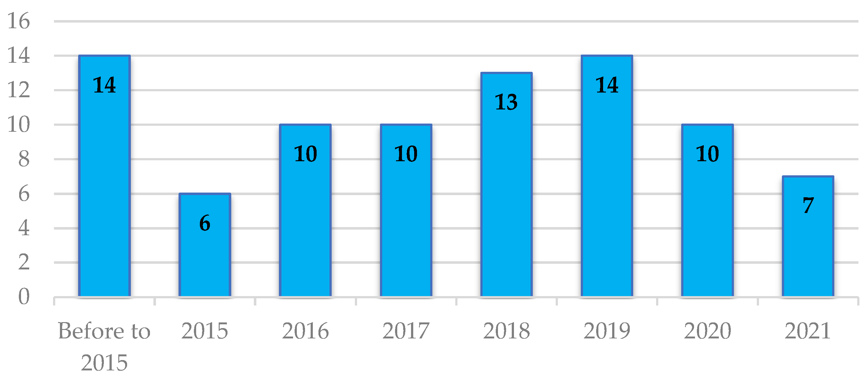
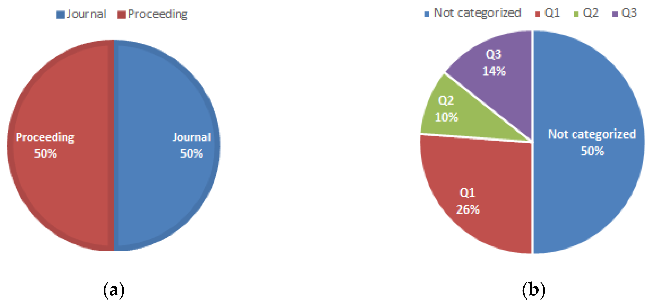
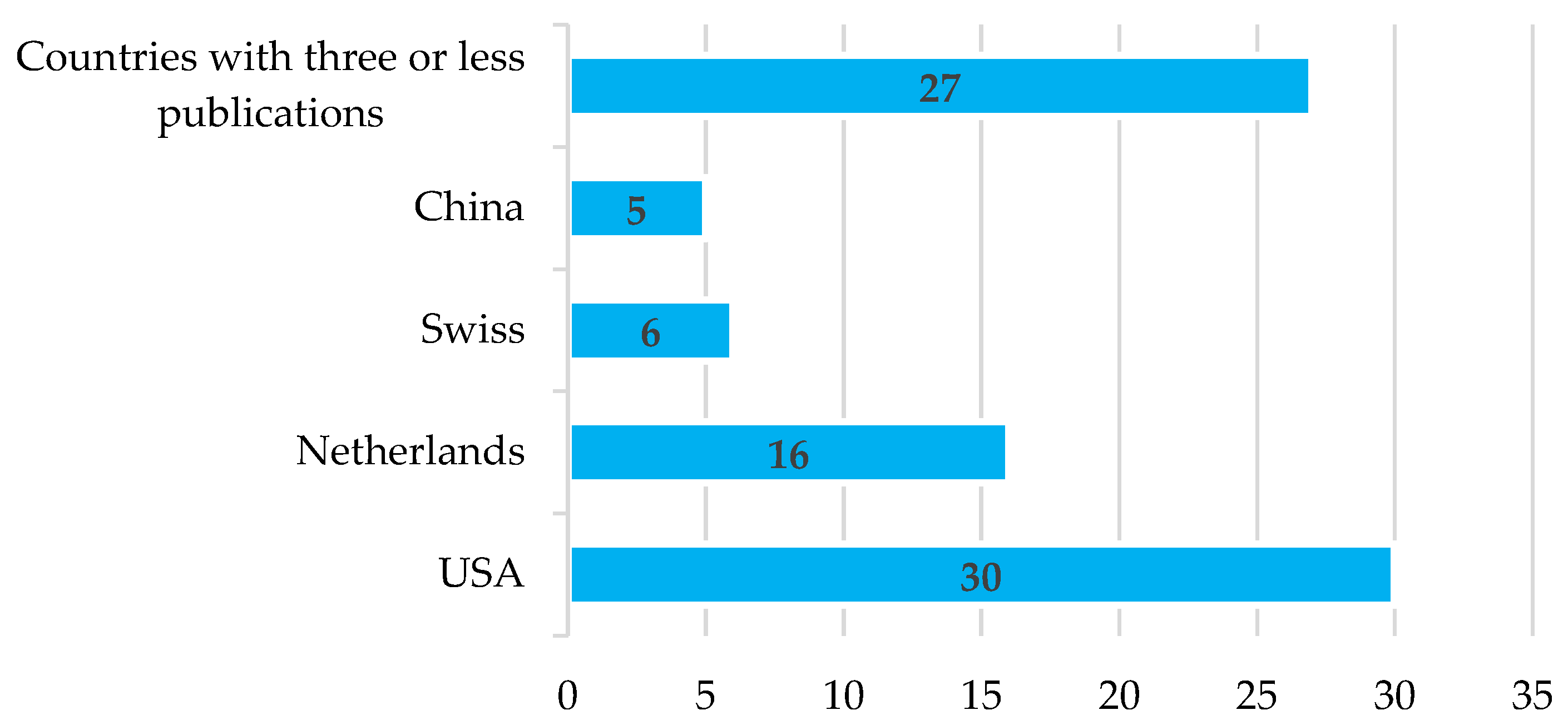
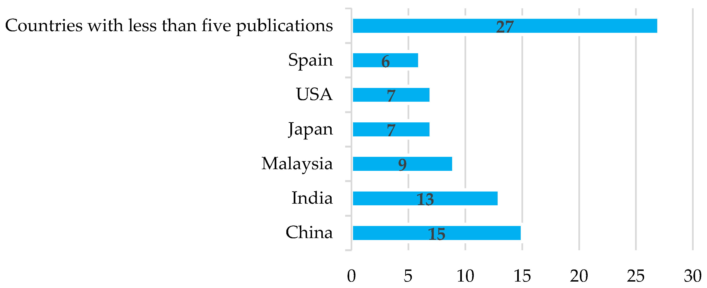
4. Scientometric Analysis
5. Technical Analysis
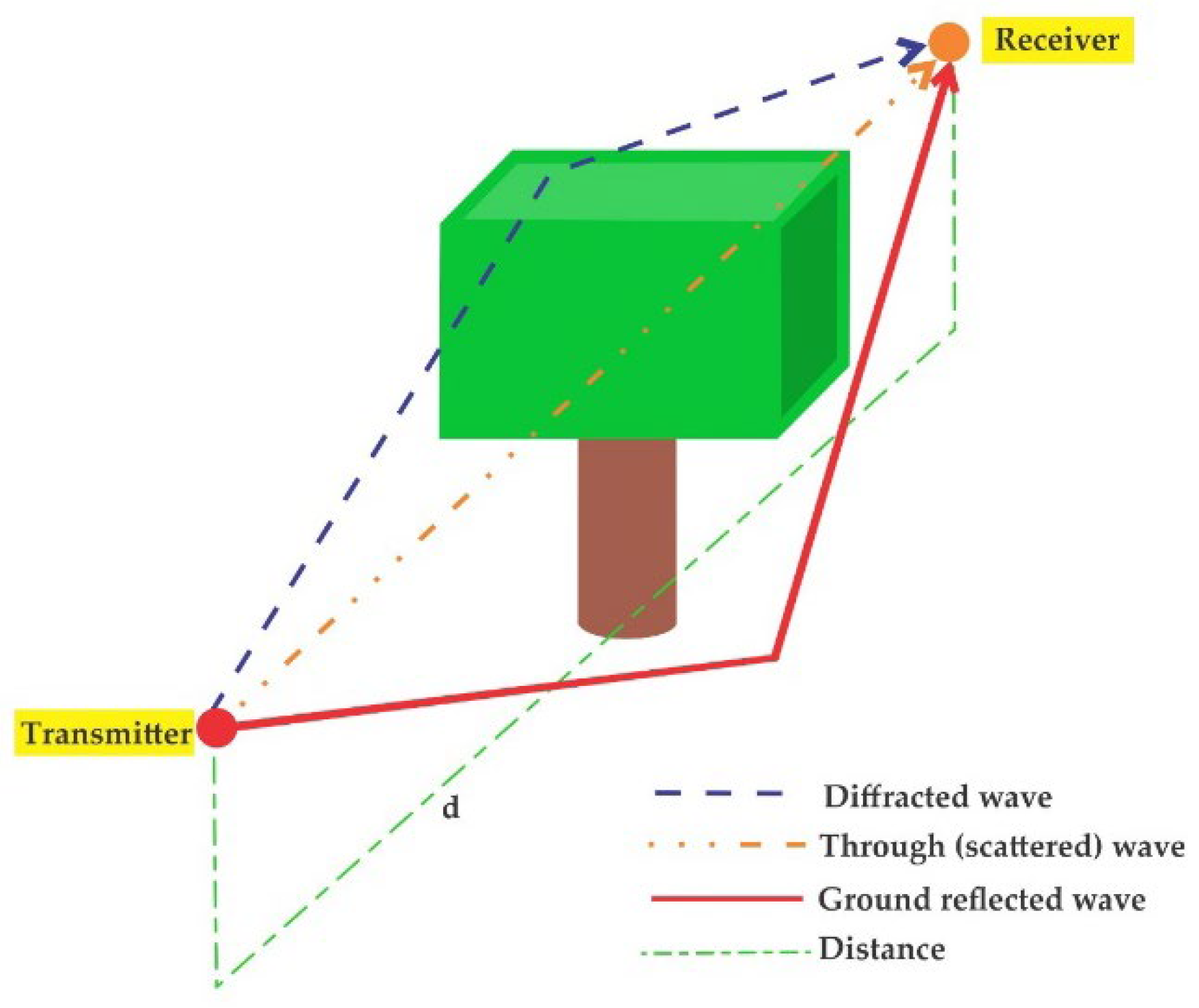
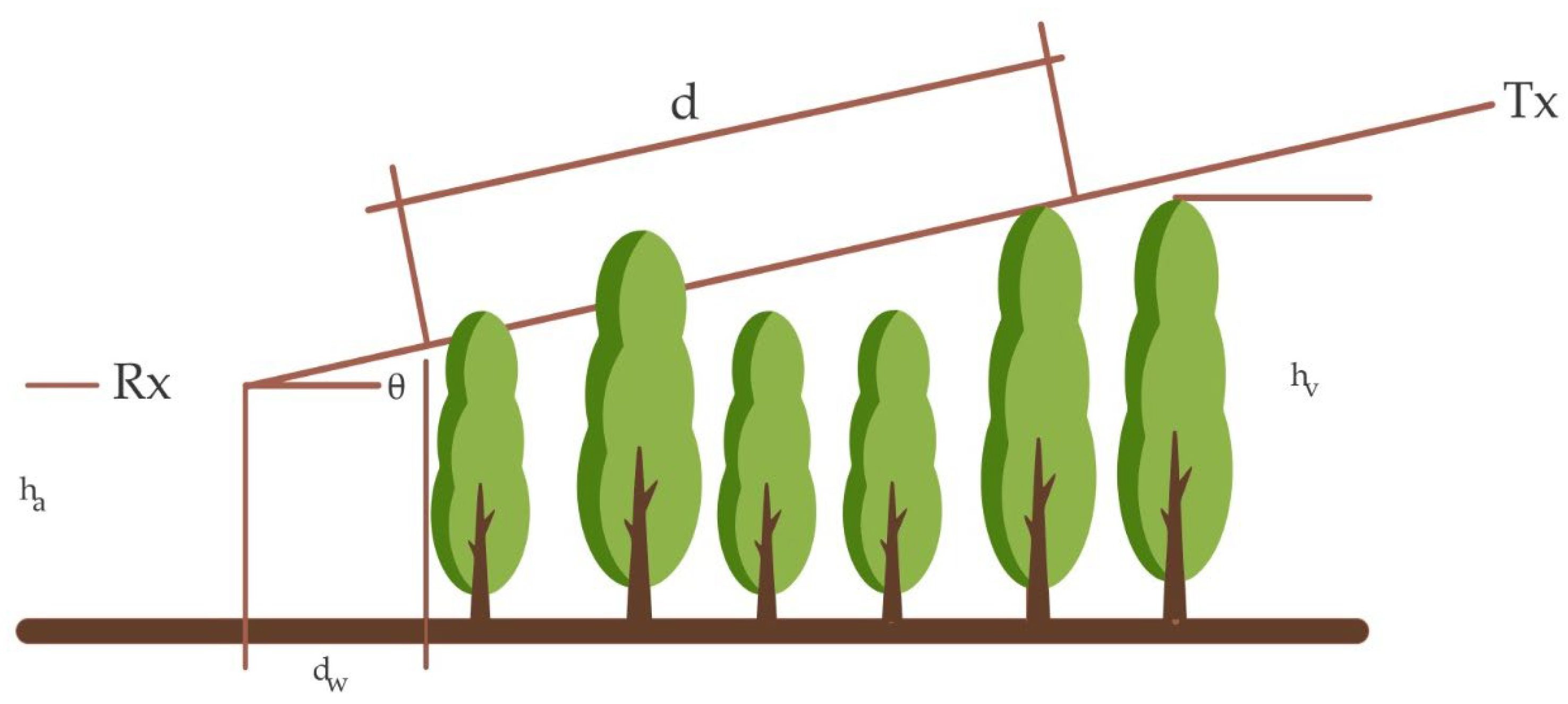
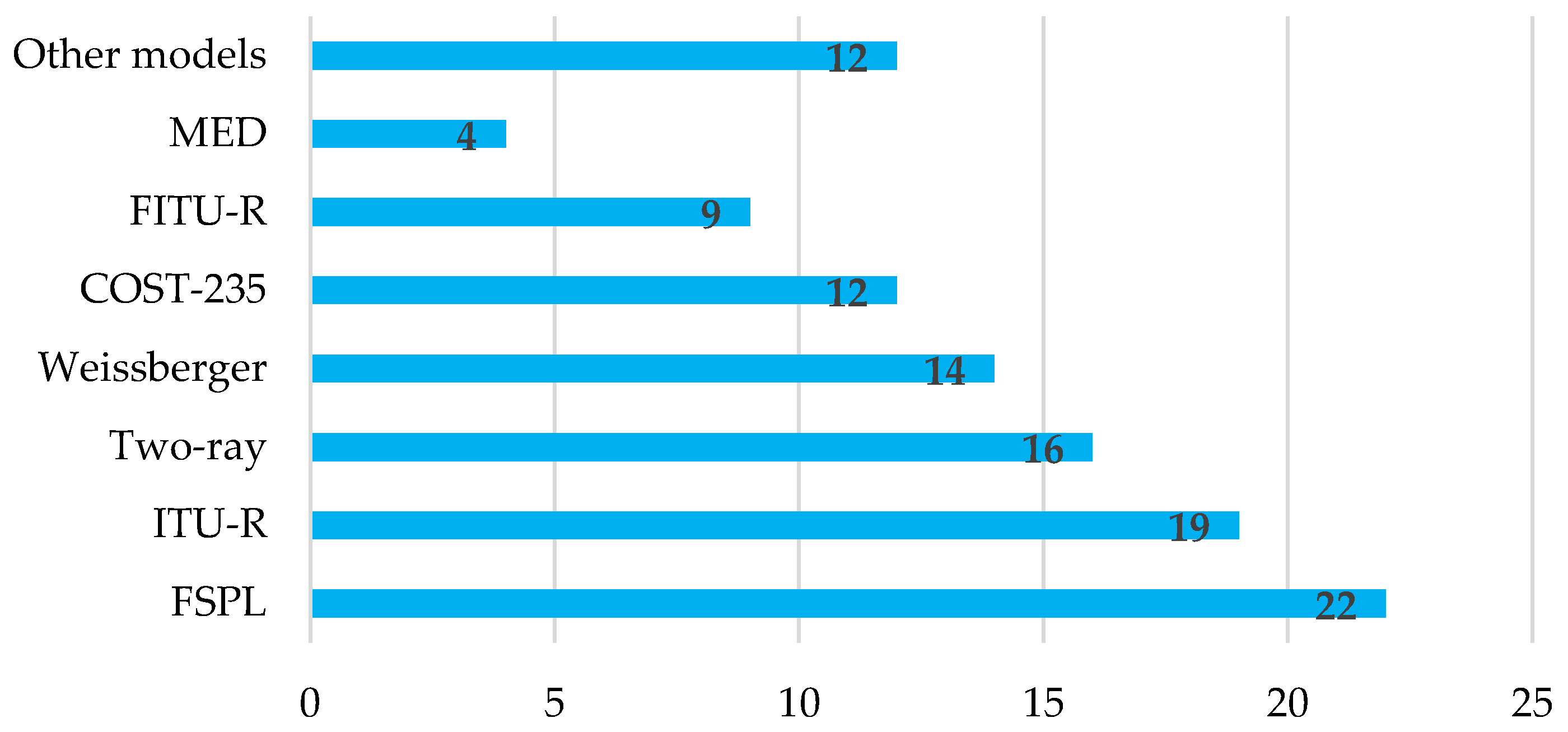
5.1. Radiowave Propagation Models for WSNs in Agricultural or Vegetated Environments
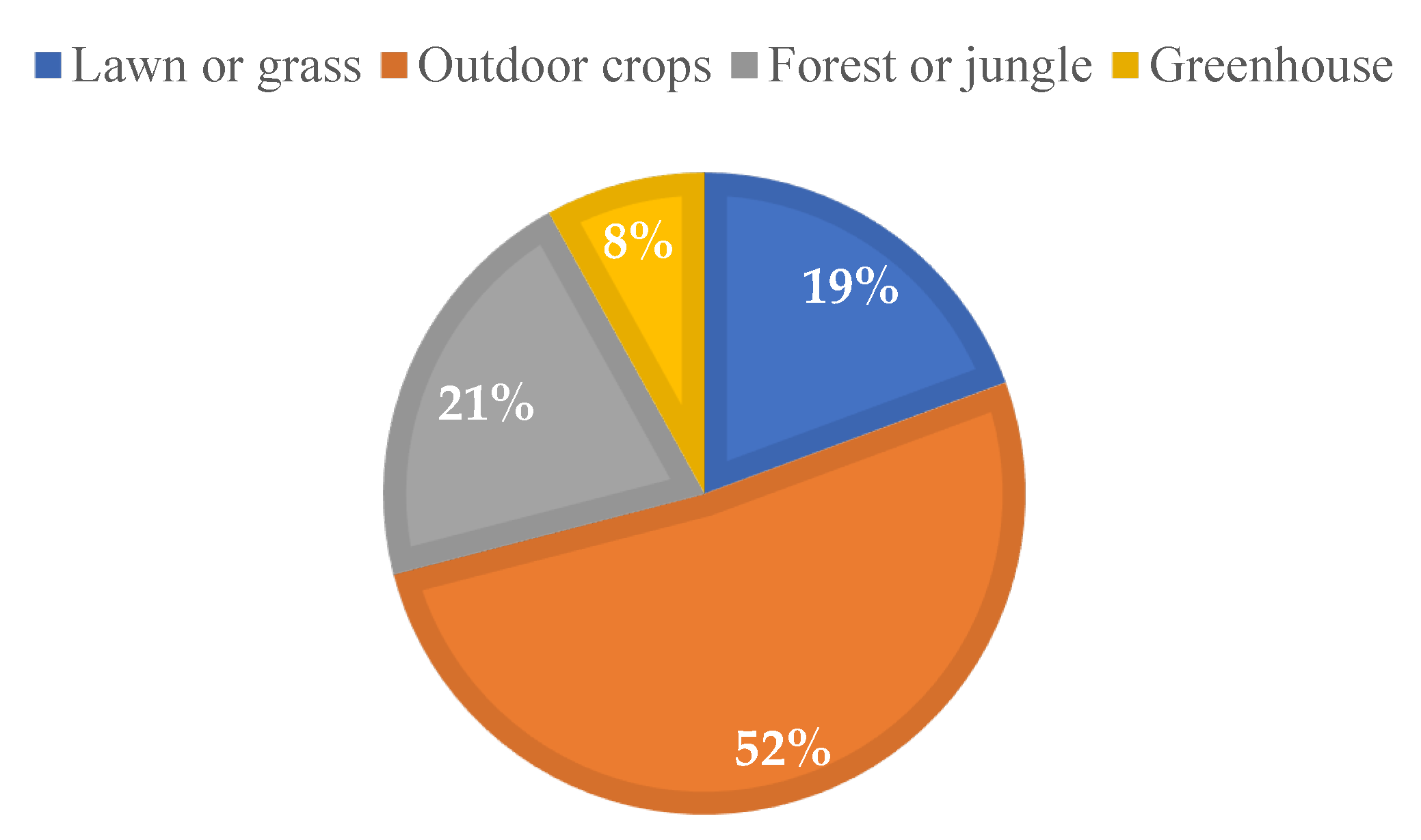
5.2. Application Scenarios for Propagation Studies
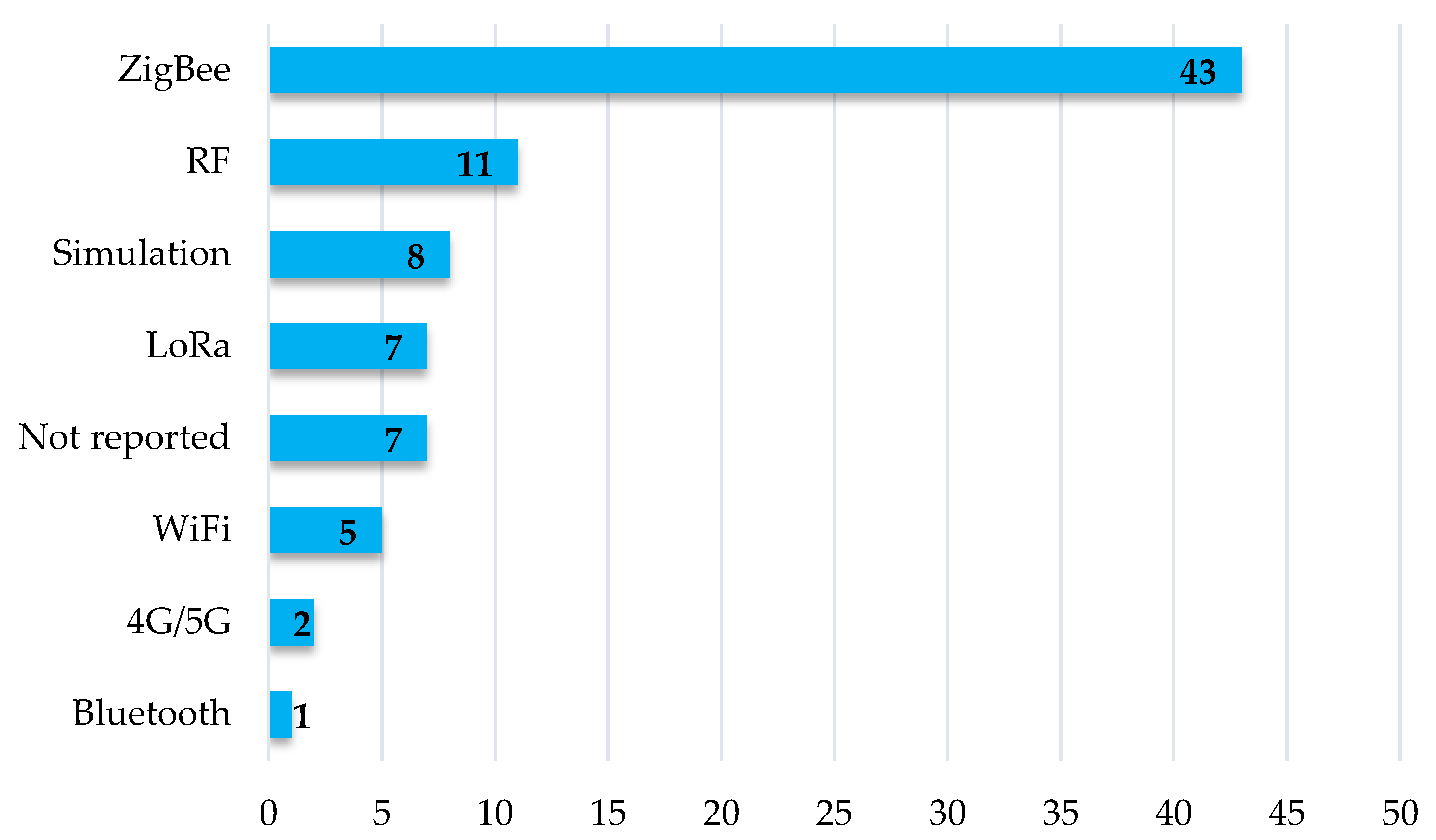
5.3. Wireless Technologies, Frequency Bands, and Tools Used
6. Discussion
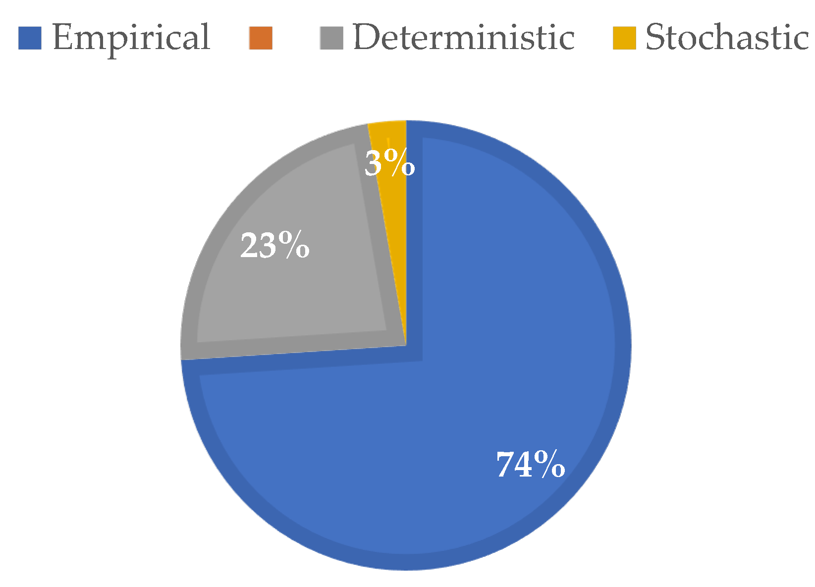
7. Results
8. Conclusions
9. Future Works
Author Contributions
Funding
Conflicts of Interest
References
- Sharma, R.P.; Ramesh, D.; Pal, P.; Tripathi, S.; Kumar, C. Crop Pest Prediction. IEEE Internet Things J. 2022, 9, 3037–3045. [Google Scholar] [CrossRef]
- Al-Qurabat, A.K.M. A Lightweight Huffman-based Differential Encoding Lossless Compression Technique in IoT for Smart Agriculture. Int. J. Comput. Digit. Syst. 2022, 11, 117–127. [Google Scholar] [CrossRef]
- Sabri, N.; Mohammed, S.S.; Fouad, S.; Syed, A.A.; Al-Dhief, F.T.; Raheemah, A. Investigation of Empirical Wave Propagation Models in Precision Agriculture. MATEC Web Conf. 2018, 150, 06020. [Google Scholar] [CrossRef]
- Khairunnniza-Bejo, S.; Ramli, N.H.; Muharam, F.M. Wireless sensor network (WSN) applications in plantation canopy areas: A review. Asian J. Sci. Res. 2018, 11, 151–161. [Google Scholar] [CrossRef]
- Thakur, D.; Kumar, Y.; Kumar, A.; Singh, P.K. Applicability of Wireless Sensor Networks in Precision Agriculture: A Review; Springer: Berlin/Heidelberg, Germany, 2019; ISBN 0123456789. [Google Scholar]
- Pal, P.; Sharma, R.P.; Tripathi, S.; Kumar, C.; Ramesh, D. 2.4 GHz RF Received Signal Strength Based Node Separation in WSN Monitoring Infrastructure for Millet and Rice Vegetation. IEEE Sens. J. 2021, 21, 18298–18306. [Google Scholar] [CrossRef]
- Barrios-Ulloa, A.; Cama-PInto, D.; Mardini-Bovea, J.; Díaz-Martínez, J.; Cama-Pinto, A. Projections of IoT Applications in Colombia Using 5G Wireless Networks. Sensors 2021, 21, 7167. [Google Scholar] [CrossRef] [PubMed]
- Cama-Pinto, D.; Damas, M.; Holgado-Terriza, J.A.; Gómez-Mula, F.; Calderín-Curtidor, A.C.; Martínez-Lao, J.A.; Cama-Pinto, A. 5G Mobile Phone Network Introduction in Colombia. Electronics 2021, 10, 922. [Google Scholar] [CrossRef]
- Dogan, H. A new empirical propagation model depending on volumetric density in citrus orchards for wireless sensornetwork applications at sub-6 GHz frequency region. Int. J. RF Microw. Comput. Eng. 2021, 31, e22778. [Google Scholar] [CrossRef]
- Gabriel, P.-E.; Butt, S.A.; Francisco, E.-O.; Alejandro, C.-P.; Maleh, Y. Performance analysis of 6LoWPAN protocol for a flood monitoring system. EURASIP J. Wirel. Commun. Netw. 2022, 2022, 16. [Google Scholar] [CrossRef]
- Cama-Pinto, A.; Piñeres-Espitia, G.; Comas-González, Z.; Vélez-Zapata, J.; Gómez-Mula, F. Design of a monitoring network of meteorological variables related to tornadoes in Barranquilla-Colombia and its metropolitan area. Ingeniare 2017, 25, 585–598. [Google Scholar] [CrossRef]
- Wu, H.; Zhang, L.; Miao, Y. The Propagation Characteristics of Radio Frequency Signals for Wireless Sensor Networks in Large-Scale Farmland. Wirel. Pers. Commun. 2017, 95, 3653–3670. [Google Scholar] [CrossRef]
- Anusha, V.S.; Nithya, G.K.; Rao, S.N. A comprehensive survey of electromagnetic propagation models. In Proceedings of the 2017 International Conference on Communication and Signal Processing (ICCSP), Chennai, India, 6–8 April 2017; pp. 1457–1462. [Google Scholar]
- Ganev, Z. Log-normal shadowing model for outdoor propagation between sensor nodes. In Proceedings of the 2018 20th International Symposium on Electrical Apparatus and Technologies (SIELA), Bourgas, Bulgaria, 3–6 June 2018; pp. 9–12. [Google Scholar]
- Kurt, S.; Tavli, B. Path-Loss Modeling for Wireless Sensor Networks: A review of models and comparative evaluations. IEEE Antennas Propag. Mag. 2017, 59, 18–37. [Google Scholar] [CrossRef]
- Tang, W.; Ma, X.; Wei, J.; Wang, Z. Measurement and analysis of near-ground propagation models under different terrains for wireless sensor networks. Sensors 2019, 19, 1901. [Google Scholar] [CrossRef]
- Vougioukas, S.; Anastassiu, H.T.; Regen, C.; Zude, M. Influence of foliage on radio path losses (PLs) for Wireless Sensor Network (WSN) planning in orchards. Biosyst. Eng. 2013, 114, 454–465. [Google Scholar] [CrossRef]
- Cama-Pinto, D.; Damas, M.; Holgado-Terriza, J.A.; Gómez-Mula, F.; Cama-Pinto, A. Path loss determination using linear and cubic regression inside a classic tomato greenhouse. Int. J. Environ. Res. Public Health 2019, 16, 1744. [Google Scholar] [CrossRef]
- Rappaport, T.S. Wireless Communications: Principles and Practice, 2nd ed.; Prentice Hall: Hoboken, NJ, USA, 2020. [Google Scholar]
- De Sales Bezerra, T.; De Sousa, J.A.R.; Da Silva Eleuterio, S.A.; Rocha, J.S. Accuracy of propagation models to power prediction in WSN ZigBee applied in outdoor environment. In Proceedings of the 6th Argentine Conference on Embedded Systems (CASE), Buenos Aires, Argentina, 12–14 August 2015; pp. 19–24. [Google Scholar]
- Barrios, A.; Arjona, R.; Álvarez, R. Comparison of Radio Propagation Models in the Suburban Area of the City of Barranquilla. Rev. Colomb. Tecnol. Av. 2018, 2, 78–85. [Google Scholar] [CrossRef]
- Shoewu, O.O.; Akinyemi, L.A.; Oborkhale, L. Towards Developing Path loss Models for Dryland and Wetland Environments. In Proceedings of the IEEE AFRICON Conference, Accra, Ghana, 25–27 September 2019. [Google Scholar] [CrossRef]
- Sevgi, L. Groundwave modeling and simulation strategies and path loss prediction virtual tools. IEEE Trans. Antennas Propag. 2007, 55, 1591–1598. [Google Scholar] [CrossRef]
- Phillips, C.; Sicker, D.; Grunwald, D. A Survey of Wireless Path Loss Prediction and Coverage Mapping Methods. IEEE Commun. Surv. Tutor. 2013, 15, 255–270. [Google Scholar] [CrossRef]
- Kamarudin, L.M.; Ahmad, R.B.; Ong, B.L.; Malek, F.; Zakaria, A.; Arif, M.A.M. Review and modeling of vegetation propagation model for wireless sensor networks using OMNeT++. In Proceedings of the 2nd International Conference on Network Applications, Protocols and Services (NETAPPS), Alor Setar, Malaysia, 22–23 September 2010; pp. 78–83. [Google Scholar]
- Rama Rao, T.; Balachander, D.; Tiwari, N. RF Propagation Measurements in Forest & Plantation Environments for Wireless Sensor Networks. In Proceedings of the 2012 IEEE International Conference on Communication Systems (ICCS), Chennai, India, 19–21 April 2012; pp. 194–198. [Google Scholar]
- Sabri, N.; Aljunid, S.A.; Salim, M.S.; Fouad, S. Wireless Sensor Network Wave Propagation in Vegetation. In Recent Trends in Physics of Material Science and Technology; Springer: Singapore, 2015; Volume 204, pp. 283–298. [Google Scholar] [CrossRef]
- Kumar, S.A.; Ilango, P. The Impact of Wireless Sensor Network in the Field of Precision Agriculture: A Review. Wirel. Pers. Commun. 2018, 98, 685–698. [Google Scholar] [CrossRef]
- Kochhar, A.; Kumar, N. Wireless sensor networks for greenhouses: An end-to-end review. Comput. Electron. Agric. 2019, 163, 104877. [Google Scholar] [CrossRef]
- Cisternas, I.; Velásquez, I.; Caro, A.; Rodríguez, A. Systematic literature review of implementations of precision agriculture. Comput. Electron. Agric. 2020, 176, 105626. [Google Scholar] [CrossRef]
- Ojha, T.; Misra, S.; Raghuwanshi, N.S. Wireless sensor networks for agriculture: The state-of-the-art in practice and future challenges. Comput. Electron. Agric. 2015, 118, 66–84. [Google Scholar] [CrossRef]
- Velásquez, J.D. A short guide to writing systematic literature reviews. Part 1. DYNA 2014, 81, 9–10. [Google Scholar] [CrossRef]
- Velásquez, J.D. A short guide to writing systematic literature reviews. Part 2. DYNA 2015, 82, 9–12. [Google Scholar] [CrossRef]
- Velásquez, J.D. A short guide to writing systematic literature reviews. Part 3. DYNA 2015, 82, 9–12. [Google Scholar] [CrossRef]
- Suter, G.W. Review papers are important and worth writing. Environ. Toxicol. Chem. 2013, 32, 1929–1930. [Google Scholar] [CrossRef]
- De-La-Hoz-Franco, E.; Ariza-Colpas, P.; Quero, J.M.; Espinilla, M. Sensor-based datasets for human activity recognition—A systematic review of literature. IEEE Access 2018, 6, 59192–59210. [Google Scholar] [CrossRef]
- ITU-R. ITU-R Recommendation P.833-7 Attenuation in Vegetation; ITU-R: Geneva, Switzerland, 2012; Volume 7. [Google Scholar]
- Anastassiu, H.T.; Vougioukas, S.; Fronimos, T.; Regen, C.; Petrou, L.; Zude, M.; Käthner, J. A computational model for path loss in wireless sensor networks in orchard environments. Sensors 2014, 14, 5118–5135. [Google Scholar] [CrossRef] [PubMed]
- Ndzi, D.L.; Harun, A.; Ramli, F.M.; Kamarudin, M.L.; Zakaria, A.; Shakaff, A.Y.M.; Jaafar, M.N.; Zhou, S.; Farook, R.S. Wireless sensor network coverage measurement and planning in mixed crop farming. Comput. Electron. Agric. 2014, 105, 83–94. [Google Scholar] [CrossRef]
- Ndzi, D.L.; Kamarudin, L.M.; Mohammad, E.A.A.; Zakaria, A.; Ahmad, R.B.; Fareq, M.M.A.; Shakaff, A.Y.M.; Jafaar, M.N. Vegetation attenuation measurements and modeling in plantations for wireless sensor network planning. Prog. Electromagn. Res. B 2011, 36, 283–301. [Google Scholar] [CrossRef]
- Balachander, D.; Rao, T.R.; Mahesh, G. RF propagation investigations in agricultural fields and gardens for wireless sensor communications. In Proceedings of the 2013 IEEE Conference on Information & Communication Technologies, Thuckalay, India, 11–12 April 2013; pp. 755–759. [Google Scholar]
- Correia Pinheiro, F.; Sampaio De Alencar, M.; Araújo Lopes, W.T.; Soares De Assis, M.; Gonçalves Leal, B. Propagation analysis for wireless sensor networks applied to viticulture. Int. J. Antennas Propag. 2017, 2017. [Google Scholar] [CrossRef]
- Azevedo, J.A.; Santos, F.E. A model to estimate the path loss in areas with foliage of trees. AEU Int. J. Electron. Commun. 2017, 71, 157–161. [Google Scholar] [CrossRef]
- Guo, X.-M.; Yang, X.-T.; Chen, M.-X.; Li, M.; Wang, Y.-A. A model with leaf area index and apple size parameters for 2.4 GHz radio propagation in apple orchards. Precis. Agric. 2015, 16, 180–200. [Google Scholar] [CrossRef]
- Wu, H.; Zhu, H.; Han, X.; Xu, W. Layout optimization for greenhouse WSN based on path loss analysis. Comput. Syst. Sci. Eng. 2021, 37, 89–104. [Google Scholar] [CrossRef]
- Olasupo, T.O.; Otero, C.E. The Impacts of Node Orientation on Radio Propagation Models for Airborne-Deployed Sensor Networks in Large-Scale Tree Vegetation Terrains. IEEE Trans. Syst. Man Cybern. Syst. 2020, 50, 256–269. [Google Scholar] [CrossRef]
- Cama-Pinto, D.; Damas, M.; Holgado-Terriza, J.A.; Arrabal-Campos, F.M.; Gómez-Mula, F.; Lao, J.A.M.; Cama-Pinto, A. Empirical model of radio wave propagation in the presence of vegetation inside greenhouses using regularized regressions. Sensors 2020, 20, 6621. [Google Scholar] [CrossRef]
- Gao, Z.; Li, W.; Zhu, Y.; Tian, Y.; Pang, F.; Cao, W.; Ni, J. Wireless channel propagation characteristics and modeling research in rice field sensor networks. Sensors 2018, 18, 3116. [Google Scholar] [CrossRef] [PubMed]
- Devarajan, N.; Gupta, S.H. Implementation and Analysis of Different Path Loss Models for Cooperative Communication. In Smart Innovations in Communication and Computational Sciences; Springer: Singapore, 2019; pp. 227–236. [Google Scholar] [CrossRef]
- Hamasaki, T. Propagation Characteristics of A 2.4GHz Wireless Sensor Module with a Pattern Antenna in Forestry and Agriculture Field. In Proceedings of the 2019 IEEE International Symposium on Radio-Frequency Integration Technology (RFIT), Nanjing, China, 28–30 August 2019; pp. 1–3. [Google Scholar]
- Alsayyari, A.; Aldosary, A. Path Loss Results for Wireless Sensor Network Deployment in a Long Grass Environment. In Proceedings of the 2018 IEEE Conference on Wireless Sensors (ICWiSe), Istanbul, Turkey, 18–20 June 2019; pp. 50–55. [Google Scholar]
- AlSayyari, A.; Kostanic, I.; Otero, C.E. An empirical path loss model for Wireless Sensor Network Deployment in a Sand Terrain Environment. In Proceedings of the 2014 IEEE World Forum on Internet of Things (WF-IoT), Seoul, Korea, 6–8 March 2014; pp. 218–223. [Google Scholar]
- Raheemah, A.; Sabri, N.; Salim, M.S.; Ehkan, P.; Ahmad, R.B. New empirical path loss model for wireless sensor networks in mango greenhouses. Comput. Electron. Agric. 2016, 127, 553–560. [Google Scholar] [CrossRef]
- Daisuke, K.; Tatsuki, T.; Toshihiko, H. Vegetation Effect in Paddy Field for a Wireless Sensor Network. In Proceedings of the 2018 USNC-URSI Radio Science Meeting (Joint with AP-S Symposium), Boston, MA, USA, 8–13 July 2018; pp. 113–114. [Google Scholar]
- Klaina, H.; Picallo, I.; Iturri, P.L.; Azpilicueta, L.; Celaya-echarri, M.; Aghzout, O. Deterministic Radio Channel Characterization for Near-Ground Wireless Sensor Networks Deployment Optimization in Smart Agriculture. In Proceedings of the 2020 14th European Conference on Antennas and Propagation (EuCAP), Copenhagen, Denmark, 15–20 March 2020; pp. 3–7. [Google Scholar]
- Hakim, G.P.N.; Alaydrus, M.; Bahaweres, R.B. Empirical approach of ad hoc path loss propagation model in realistic forest environments. In Proceedings of the 2016 International Conference on Radar, Antenna, Microwave, Electronics and Telecommunications (ICRAMET), Jakarta, Indonesia, 3–5 October 2016; pp. 139–143. [Google Scholar] [CrossRef]
- Cama-Pinto, A.; Piñeres-Espitia, G.; Caicedo-Ortiz, J.; Ramírez-Cerpa, E.; Betancur-Agudelo, L.; Gómez-Mula, F. Received strength signal intensity performance analysis in wireless sensor network using Arduino platform and XBee wireless modules. Int. J. Distrib. Sens. Netw. 2017, 13, 2–8. [Google Scholar] [CrossRef]
- Shutimarrungson, N.; Wuttidittachotti, P. Realistic propagation effects on wireless sensor networks for landslide management. EURASIP J. Wirel. Commun. Netw. 2019, 94. [Google Scholar] [CrossRef]
- Artemenko, O.; Rubina, A.; Nayak, A.H.; Baptist, S.; Mitschele-thiel, A. Evaluation of di ff erent signal propagation models for a mixed indoor-outdoor scenario using empirical data. EAI Endorsed Trans. Mob. Commun. Appl. 2016, 2, 94. [Google Scholar] [CrossRef]
- Stewart, J.; Stewart, R.; Kennedy, S. Internet of Things—Propagation Modelling for Precision Agriculture Applications. In Proceedings of the IEEE International Conference Image Information Processing, Chicago, IL, USA, 26–28 April 2017; pp. 1–8. [Google Scholar]
- Jawad, H.M.; Jawad, A.M.; Nordin, R.; Gharghan, S.K.; Abdullah, N.F.; Ismail, M.; Abu-Alshaeer, M.J. Accurate Empirical Path-Loss Model Based on Particle Swarm Optimization for Wireless Sensor Networks in Smart Agriculture. IEEE Sens. J. 2020, 20, 552–561. [Google Scholar] [CrossRef]
- Picallo, I.; Klaina, H.; Lopez-Iturri, P.; Aguirre, E.; Celaya-Echarri, M.; Azpilicueta, L.; Eguizábal, A.; Falcone, F.; Alejos, A. A radio channel model for D2D communications blocked by single trees in forest environments. Sensors 2019, 19, 4606. [Google Scholar] [CrossRef] [PubMed]
- Chen, Y.; Chamadiya, B. Propagation model for vehicle to vehicle LOS communication in foliage scenario. In Proceedings of the 2014 International Conference on Connected Vehicles and Expo, ICCVE, Vienna, Austria, 3–7 November 2014; pp. 1120–1125. [Google Scholar]
- Rao, T.R.; Balachander, D.; Tiwari, N.; Prasad, M.V.S.N. Ultra-high frequency near-ground short-range propagation measurements in forest and plantation environments for wireless sensor networks. IET Wirel. Sens. Syst. 2013, 3, 80–84. [Google Scholar] [CrossRef]
- Rahim, H.M.; Leow, C.Y.; Rahman, T.A. Millimeter wave propagation through foliage: Comparison of models. In Proceedings of the 2015 IEEE 12th Malaysia International Conference on Communications, MICC, Kuching, Malaysia, 23–25 November 2015; pp. 236–240. [Google Scholar]
- Zhang, J.; Li, C.; Yu, J.; Li, F.; Chang, F.; Chen, Y.; Chen, W. Path Loss Analysis and Model Selection in Forest City Environment at 5.9 GHz. In Proceedings of the 2nd IEEE Advanced Information Management, Communicates, Electronic and Automation Control Conference, IMCEC, Xi’an, China, 25–27 May 2018; pp. 516–520. [Google Scholar]
- Rao, Y.; Jiang, Z.H.; Lazarovitch, N. Investigating signal propagation and strength distribution characteristics of wireless sensor networks in date palm orchards. Comput. Electron. Agric. 2016, 124, 107–120. [Google Scholar] [CrossRef]
- Castellanos, G.; Teuta, G. Path loss model in amazonian border region for VHF and UHF television bands. In Proceedings of the 2017 IEEE-APS Topical Conference on Antennas and Propagation in Wireless Communications, APWC, Verona, Italy, 11–15 September 2017; pp. 137–140. [Google Scholar]
- Oda, E.; Kawauchi, K.; Hamasaki, T. Support Application for Configuring Optimal Relay Nodes in Wireless Sensor Networks. In Proceedings of the 2021 IEEE Topical Conference on Wireless Sensors and Sensor Networks, WiSNeT, Diego, CA, USA, 17–20 January 2021; pp. 19–22. [Google Scholar]
- Kamarudin, L.M.; Ahmad, R.B.; Ndzi, D.; Zakaria, A.; Ong, B.L.; Kamarudin, K.; Harun, A.; Mamduh, S.M. Modeling and simulation of WSNs for agriculture applications using dynamic transmit power control algorithm. In Proceedings of the 3rd Inernational Conference on Intelligent Systems Modelling and Simulation, Kota Kinabalu, Malaysia, 8–10 February 2012; pp. 616–621. [Google Scholar] [CrossRef]
- Myagmardulam, B.; Tadachika, N.; Takahashi, K.; Miura, R.; Ono, F.; Kagawa, T. Path Loss Prediction Model Development in a Mountainous Forest Environment. IEEE Open J. Commun. Soc. 2021, 2, 2494–2501. [Google Scholar] [CrossRef]
- Yamaoka, Y.; Hamasaki, T.; Kuramoto, D. 2.4 GHz RF Propagation Measurements and Modeling in a Paddy Field for a Wireless Sensor Network. In Proceedings of the 2019 IEEE-APS Topical Conference on Antennas and Propagation in Wireless Communications (APWC), Granada, Spain, 9–13 September 2019; pp. 34–35. [Google Scholar]
- Brinkhoff, J.; Hornbuckle, J. Characterization of WiFi signal range for agricultural WSNs. In Proceedings of the 2017 23rd Asia-Pacific Conference on Communications: Bridging the Metropolitan and the Remote, (APCC), Perth, Australia, 11–13 December 2018; pp. 1–6. [Google Scholar]
- Pan, H.; Shi, Y.; Wang, X.; Li, T. Modeling wireless sensor networks radio frequency signal loss in corn environment. Multimed. Tools Appl. 2017, 76, 19479–19490. [Google Scholar] [CrossRef]
- Wu, H.; Miao, Y.; Li, F.; Zhu, L. Empirical modeling and evaluation of multi-path radio channels on wheat farmland based on communication quality. Trans. ASABE 2016, 59, 759–767. [Google Scholar] [CrossRef]
- Liu, H.; Meng, Z.; Wang, M. A wireless sensor network for cropland environmental monitoring. In Proceedings of the International Conference on Networks Security, Wireless Communications and Trusted Computing (NSWCTC), Wuhan, China, 25–26 April 2009; Volume 1, pp. 65–68. [Google Scholar] [CrossRef]
- Olasupo, T.O.; Alsayyari, A.; Otero, C.E.; Olasupo, K.O.; Kostanic, I. Empirical path loss models for low power wireless sensor nodes deployed on the ground in different terrains. In Proceedings of the 2017 IEEE Jordan Conference on Applied Electrical Engineering and Computing Technologies (AEECT), Aqaba, Jordan, 11–13 October 2017; pp. 1–8. [Google Scholar]
- Olasupo, T.O.; Otero, C.E.; Olasupo, K.O.; Kostanic, I. Empirical path loss models for wireless sensor network deployments in short and tall natural grass environments. IEEE Trans. Antennas Propag. 2016, 64, 4012–4021. [Google Scholar] [CrossRef]
- Perez, G.E.; Alsayyari, A.; Kostanic, I. Comparison of the propagation loss of a real-life wireless sensor network and its complimentary simulation model. In Proceedings of the 2015 IEEE 17th International Conference on High Performance Computing and Communications, 2015 IEEE 7th International Symposium on Cyberspace Safety and Security, and 2015 IEEE 12th International Conference on Embedded Software and Systems, New York, NY, USA, 24–26 August 2015; pp. 1832–1837. [Google Scholar]
- Srisooksai, T.; Kaemarungsi, K.; Takada, J.; Saito, K. Radio propagation measurement and characterization in outdoor tall food grass agriculture field for wireless sensor network at 2.4 GHz band. Prog. Electromagn. Res. C 2018, 88, 43–58. [Google Scholar] [CrossRef]
- Iswandi; Nastiti, H.T.; Praditya, I.E.; Mustika, I.W. Evaluation of XBee-Pro transmission range for Wireless Sensor Network’s node under forested environments based on Received Signal Strength Indicator (RSSI). In Proceedings of the 2nd International Conference on Science and Technology-Computer, ICST, Yogyakarta, Indonesia, 27–28 October 2016; pp. 56–60. [Google Scholar]
- Gay-Fernández, J.A.; Cuiñas, I. Peer to peer wireless propagation measurements and path-loss modeling in vegetated environments. IEEE Trans. Antennas Propag. 2013, 61, 3302–3311. [Google Scholar] [CrossRef]
- Mathew, K.; Tabassum, M. Analysis of bluetooth and zigbee signal penetration and interference in foliage. In Proceedings of the International MultiConference of Engineers and Computer Scientists (IMECS); Hong Kong, China, 16–18 March 2016, Volume 2, pp. 547–552.
- He, Y.; Zhang, W.; Jiang, N.; Luo, X. The research of wireless sensor network channel propagation model in the wild environment. In Proceedings of the 9th International Conference on P2P, Parallel, Grid, Cloud and Internet Computing 3PGCIC, Guangdong, China, 8–10 November 2014; pp. 227–231. [Google Scholar] [CrossRef]
- Liu, L.; Yao, Y.; Cao, Z.; Zhang, M. DeepLoRa: Learning Accurate Path Loss Model for Long Distance Links in LPWAN. In Proceedings of the IEEE INFOCOM, Virtual, 10–13 May 2021. [Google Scholar]
- Manpreet; Malhotra, J. ZigBee technology: Current status and future scope. In Proceedings of the 2015 International Conference on Computer and Computational Sciences (ICCCS), Greater Noida, India, 27–29 January 2015; pp. 163–169. [Google Scholar] [CrossRef]
- Sadowski, S.; Spachos, P. Wireless technologies for smart agricultural monitoring using internet of things devices with energy harvesting capabilities. Comput. Electron. Agric. 2020, 172, 105338. [Google Scholar] [CrossRef]
- Danbatta, S.J.; Varol, A. Comparison of Zigbee, Z-Wave, Wi-Fi, and Bluetooth Wireless Technologies Used in Home Automation. In Proceedings of the 7th International Symposium on Digital Forensics and Security (ISDFS), Barcelos, Portugal, 10–12 June 2019; pp. 1–5. [Google Scholar]
- Gloria, A.; Cercas, F.; Souto, N. Comparison of communication protocols for low cost Internet of Things devices. In Proceedings of the South-East Europe Design Automation, Computer Engineering, Computer Networks and Social Media Conference, SEEDA-CECNSM, Kastoria, Greece, 23–25 September 2017. [Google Scholar]
- Peng, Y.L.; Li, P.P.; Wang, J.Z.; Hu, Y.G.; Lin, Y.F. Propagation characteristics of 2.4 GHz wireless channel at different directions and heights in tea plantation. Appl. Mech. Mater. 2013, 325–326, 1697–1701. [Google Scholar] [CrossRef]
- Benaissa, S.; Plets, D.; Tanghe, E.; Verloock, L.; Martens, L.; Hoebeke, J.; Sonck, B.; Tuyttens, F.A.M.; Vandaele, L.; Stevens, N.; et al. Experimental characterisation of the off-body wireless channel at 2.4 GHz for dairy cows in barns and pastures. Comput. Electron. Agric. 2016, 127, 593–605. [Google Scholar] [CrossRef]
- Zhang, W.; He, Y.; Liu, F.; Miao, C.; Sun, S.; Liu, C.; Jin, J. Research on WSN channel fading model and experimental analysis in orchard environment. In Computer and Computing Technologies in Agriculture V. CCTA 2011; IFIP Advances in Information and Communication Technology Book Series (IFIPAICT, Volume 369); Springer: Berlin/Heidelber, Germany, 2012; pp. 326–333. [Google Scholar] [CrossRef]
- Samijayani, O.N.; Mujadin, A.; Darwis, R.; Astharini, D.; Rahmatia, S. Hybrid ZigBee and WiFi Wireless Sensor Networks for Hydroponic Monitoring. In Proceedings of the 2020 International Conference on Electrical, Communication, and Computer Engineering (ICECCE), Istanbul, Turkey, 12–13 June 2020; pp. 1–4. [Google Scholar]
- Botella-campos, M.; Parra, L.; Sendra, S.; Lloret, J. WLAN IEEE 802. 11b/g/n Coverage Study for Rural Areas. In Proceedings of the 2020 International Conference on Control, Automation and Diagnosis (ICCAD), Paris, France, 7–9 October 2020; pp. 1–6. [Google Scholar]
- Lavanya, U.; Mupparaju, S.; Patnala, P.; Anugu, P.R.; Surendran, S. Model Selection for Path Loss Prediction in Wireless Networks. In Proceedings of the 2020 International Conference on Communication and Signal Processing (ICCSP), Chennai, India, 28–30 July 2020; pp. 1490–1493. [Google Scholar]
- Lora Alliance What Is LoRaWAN Specification. Available online: https://lora-alliance.org/about-lorawan/ (accessed on 1 February 2021).
- Amali, K.; Sharil, M.; Devi, J. Impact of foliage on LoRa 433 MHz propagation in tropical environment Impact of Foliage on LoRa 433MHz Propagation in Tropical Environment. In AIP Conference Proceedings; AIP Publishing LLC: Melville, NY, USA, 2019; Volume 20009, pp. 1–7. [Google Scholar]
- Avila-Campos, P.; Astudillo-Salinas, F.; Vazquez-Rodas, A. Evaluation of LoRaWAN Transmission Range for Wireless Sensor Networks in Riparian Forests. In Proceedings of the 22nd International ACM Conference on Modeling, Analysis and Simulation of Wireless and Mobile Systems (MSWiM), Miami, FL, USA, 25 November 2019; pp. 199–206. [Google Scholar]
- Zarnescu, A.; Ungurelu, R.; Secere, M.; Varzaru, G.; Mihailescu, B. Implementing a large LoRa network for an agricultural application. In Proceedings of the 7th International Conference on Energy Efficiency and Agricultural Engineering (EE&AE), Ruse, Bulgaria, 12–14 November 2020; pp. 4–8. [Google Scholar] [CrossRef]
- Anzum, R. Factors that affect LoRa Propagation in Foliage Factors that affect LoRa Propagation Foliage Medium Factors that affect LoRa Propagation in Foliage Factors that affect LoRa Propagation Foliage Medium Factors that affect LoRa Propagation in Foliage Medium. Procedia Comput. Sci. 2021, 194, 149–155. [Google Scholar] [CrossRef]
- Anzum, R.; Hadi Habaebi, M.; Islam, R.; Hakim, G.P.N. Modeling and Quantifying Palm Trees Foliage Loss using LoRa Radio Links for Smart Agriculture Applications. In Proceedings of the 7th International Conference on Smart Instrumentation, Measurement and Applications (ICSIMA), Bandung, Indonesia, 23–25 August 2021; pp. 105–110. [Google Scholar] [CrossRef]
- Phaiboon, S.; Phokharatkul, P. An Empirical Path Loss Model for Wireless Sensor Network Placement in Banana Plantation. In Proceedings of the Progress in Electromagnetics Research Symposium, Hangzhou, China, 21–25 November 2021; pp. 354–357. [Google Scholar]
- AlSayyari, A.; Kostanic, I.; Otero, C.E. An Empirical Path Loss Model for Wireless Sensor Network Deployment in a Dense Tree Environment. In Proceedings of the 2017 IEEE Sensors Applications Symposium (SAS), Glassboro, NJ, USA, 13–15 March 2017; pp. 1–6. [Google Scholar]
- Alsayyari, A.; Aldosary, A. Path loss results for wireless sensor network deployment in a sparse tree environment. In Proceedings of the 2019 International Symposium on Networks, Computers and Communications (ISNCC), Istanbul, Turkey, 18–20 June 2019; pp. 1–6. [Google Scholar] [CrossRef]
- Xu, X.; Zhang, Z.; Xu, Y.; Yang, Z.; Chen, Y.; Liang, Z.; Zhou, J.; Zheng, J. Measurement and Analysis of Wireless propagative Model of 433MHz and 2.4GHz Frequency in Southern China Orchards. IFAC-PapersOnLine 2018, 51, 695–699. [Google Scholar] [CrossRef]
- Navarro, A.; Guevara, D.; Florez, G.A. An Adjusted Propagation Model for Wireless Sensor Networks in Corn Fields. In Proceedings of the 2020 XXXIIIrd General Assembly and Scientific Symposium of the International Union of Radio Science, Rome, Italy, 29 August–5 September 2020; pp. 1–3. [Google Scholar]


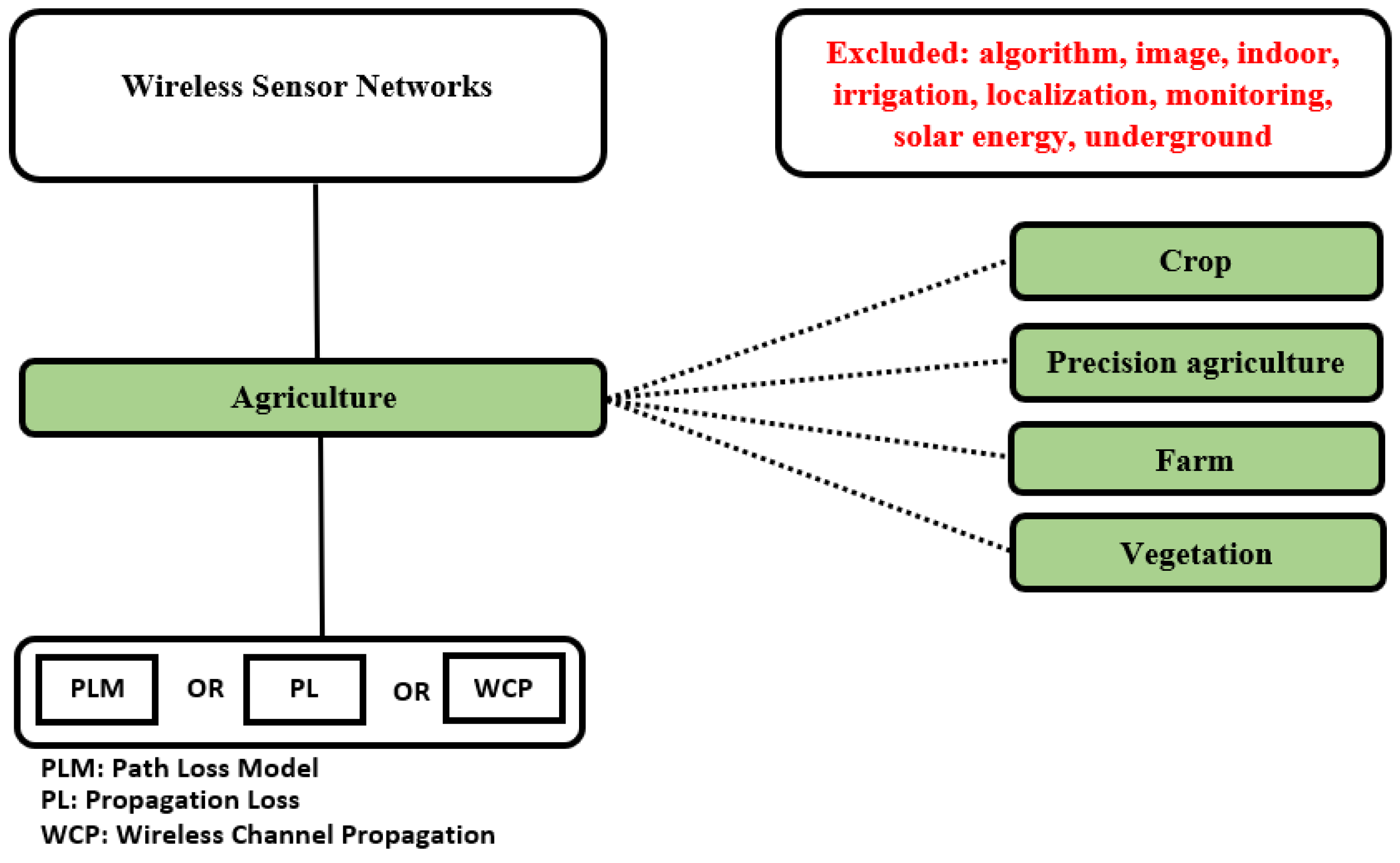
| Thematic Axis 1 | Thematic Axis 2 | Thematic Axis 3 | Exclusion Criteria |
|---|---|---|---|
| Agriculture | WSN | Path loss | Algorithm |
| Crop | Path loss model | Image | |
| Farm | Wave propagation | Indoor | |
| Vegetation | Irrigation | ||
| Localization | |||
| Monitoring | |||
| Solar energy | |||
| Combinations | |||
| Link 1: | Axis 1 AND Axis 2 | ||
| Link 2: | Axis 1 AND Axis 2 AND NOT Exclusion criteria | ||
| Link 3: | Axis 1 AND Axis 2 AND Axis 3 | ||
| Link 4: | Axis 1 AND Axis 2 AND Axis 3 NOT Exclusion criteria | ||
| Link 5: | Axis 2 AND Axis 3 | ||
| Link 6: | Axis 2 AND Axis 3 NOT Exclusion criteria | ||
| Publishing | Number of Posts | Country | Type | ISSN | Quartile in SJR | Quartile in JCR |
|---|---|---|---|---|---|---|
| Computers and Electronics in Agriculture | 9 | Netherlands | Journal | 1681699 | Q1 | Q1 |
| Sensors | 5 | Switzerland | Journal | 14243210 | Q2 | Q1 |
| Progress in Electromagnetics Research C | 3 | USA | Journal | 19378718 | Q3 | Q3 |
| Wireless Personal Communications | 3 | Netherlands | Journal | 1572834X | Q3 | Q4 |
| Model | Vegetative Model | Antenna Height | Antenna Gain | Conditions | Observations | References |
|---|---|---|---|---|---|---|
| MED | Yes | No | No | d < 400 m 200 MHz < f < 95 GHz | Applicable in communication links obstructed by dense, dry, leafy trees; present in temperate latitude forests. | [27,38,39,40,63] |
| ITU-R | Yes | No | No | d < 400 m 200 MHz < f < 95 GHz For f above 1 GHz, it only considers the diffracted components around the vegetation and from above, in addition to the component reflected from the ground. | It is proposed for cases where the transmitting or receiving antenna is located near a small grove of trees, allowing most of the signal to propagate through the vegetation. | [3,12,27,40,41,42,46,53,64,65,66] |
| COST-235 | Yes | No | No | 200 MHz < f < 95 GHz | Consider the presence and absence of leaves on trees. It can be used in vegetation scenarios up to 200 meters wide. | [3,12,18,26,41,46,53,60,67,68] |
| FITU-R | Yes | No | No | d < 400 m | Consider the presence and absence of leaves on trees. Suitable for modeling the propagation of radio waves in different seasons of the year. | [3,9,53,60,63] |
| Weissberger | Yes | No | No | d < 400 m 230 MHz < f < 95 GHz | Useful when the path between the transmitter and the receiver is occupied by dense vegetation consisting of trees with low humidity. | [3,12,18,26,40,41,42,46,53,64] |
| FSPL | No | No | Yes | d >> λ | This model does not consider the mechanisms of radio wave propagation (e.g., reflection, diffraction, refraction, absorption). It is used as a reference to compare the performance of different wireless communication technologies. It is also a complement to vegetation models to calculate losses over the entire channel path. | [15,16,26,39,46,48,56,57,69,70,71] |
| Two-Ray | No | Yes | Yes | d >> ht + hr | This model considers the effects of the ground and the reflection of the ray LOS (line-of-sight). Useful for modeling propagation over long distances. It is also a complement to vegetation models to calculate losses over the entire channel path. | [15,16,45,46,48,69] |
| Technology | Frequency Bands | Speed Rate | Coverage Range (Typical) | Energy Consumption |
|---|---|---|---|---|
| Bluetooth | 2.4 GHz | 720 kbps–1 Mbps | 1–10 m | Low |
| LoRaWAN | 433 MHz, 868 MHz | 250 bps–50 kbps | >10 km | Low |
| WiFi | 2.4 GHz, 5 GHz | 1.2 Mbps–54 Mbps | Hasta 100 m | High |
| Zigbee | 870 MHz, 902–928 MHz, 2.4 GHz | 20 kbps–250 kbps | 10 m–1.6 km | Low |
| Canon | Measure |
|---|---|
| Models | COST-235, ITU-R, FITU-R, Weissberger, MED, FSPL, Two-ray |
| Characterization of attenuation | Loss vs. distance RSSI vs. distance |
| Track predictions | Graphical method RMSE MAPE R2 |
| Prediction effectiveness | Follow measurements closely Overestimate Underestimate |
| Reference | Models | Environment | Technology | Summary of Results |
|---|---|---|---|---|
| [16] | FSPL, Two-Ray | Grass | RF equipment |
|
| [12] | COST-235, ITU-R, Weissberger | Agricultural fields | Zigbee |
|
| [27] | COST-235, FSPL, Weissberger | Agricultural fields | RF equipment |
|
| [38] | ITU-R | Agricultural fields | Zigbee |
|
| [40] | FITU-R, ITU-R, Weissberger | Agricultural fields | RF equipment |
|
| [39] | FSPL, MED | Agricultural fields | Zigbee |
|
| [42] | ITU-R, Weissberger | Agricultural fields | Zigbee |
|
| [43] | COST-235, FITU-R, FSPL, ITU-R | Agricultural fields | RF equipment |
|
| [44] | COST-235, FITU-R, Weissberger | Agricultural fields | Zigbee |
|
| [18] | COST-235, FSPL, ITU-R, Two-Ray, Weissberger | Greenhouse | Zigbee |
|
| [46] | COST-235, FSPL, ITU-R, Two-Ray, Weissberger | Forest or jungle | Zigbee |
|
| [48] | FSPL, Two-Ray | Agricultural fields | Zigbee |
|
| [53] | COST-235, FITU-R, FSPL, ITU-R, Two-Ray, Weissberger | Greenhouse | Zigbee |
|
| [56] | FSPL | Forest or jungle | WiFi |
|
| [58] | COST-235, FITU-R, FSPL, Weissberger | Forest or jungle | RF equipment |
|
| [60] | COST-235, FITU-R | Forest or jungle | WiFi |
|
| [82] | FSPL, ITU-R | Forest or jungle | RF equipment |
|
| [67] | COST-235, FITU-R, ITU-R, MED | Agricultural fields | Zigbee |
|
| [104] | FSPL, Two-Ray | Forest and grass | Zigbee |
|
| [106] | FSPL, ITU-R, Two-Ray | Agricultural fields | Zigbee |
|
| Reference | Environment | Technology | Summary of Results |
|---|---|---|---|
| [43] | Forest or jungle | RF equipment |
|
| [44] | Agricultural field | Zigbee |
|
| [48] | Agricultural field | Zigbee |
|
| [60] | Forest or jungle | WiFi |
|
| [38] | Agricultural field | Zigbee |
|
| [18] | Greenhouse | Zigbee |
|
| [50] | Agricultural field | Zigbee |
|
| [62] | Forest or jungle | RF equipment |
|
| [77] | Grass | Zigbee |
|
| [104] | Forestry and turf | Zigbee |
|
| [105] | Forest or jungle | Zigbee |
|
| [106] | Agricultural field | RF equipment |
|
Publisher’s Note: MDPI stays neutral with regard to jurisdictional claims in published maps and institutional affiliations. |
© 2022 by the authors. Licensee MDPI, Basel, Switzerland. This article is an open access article distributed under the terms and conditions of the Creative Commons Attribution (CC BY) license (https://creativecommons.org/licenses/by/4.0/).
Share and Cite
Barrios-Ulloa, A.; Ariza-Colpas, P.P.; Sánchez-Moreno, H.; Quintero-Linero, A.P.; De la Hoz-Franco, E. Modeling Radio Wave Propagation for Wireless Sensor Networks in Vegetated Environments: A Systematic Literature Review. Sensors 2022, 22, 5285. https://doi.org/10.3390/s22145285
Barrios-Ulloa A, Ariza-Colpas PP, Sánchez-Moreno H, Quintero-Linero AP, De la Hoz-Franco E. Modeling Radio Wave Propagation for Wireless Sensor Networks in Vegetated Environments: A Systematic Literature Review. Sensors. 2022; 22(14):5285. https://doi.org/10.3390/s22145285
Chicago/Turabian StyleBarrios-Ulloa, Alexis, Paola Patricia Ariza-Colpas, Hernando Sánchez-Moreno, Alejandra Paola Quintero-Linero, and Emiro De la Hoz-Franco. 2022. "Modeling Radio Wave Propagation for Wireless Sensor Networks in Vegetated Environments: A Systematic Literature Review" Sensors 22, no. 14: 5285. https://doi.org/10.3390/s22145285