
Prototype Regularized Manifold Regularization Technique for Semi-Supervised Online Extreme Learning Machine

 , ,
, ,
Abstract
:1. Introduction
- (1)
- A prototype regularized manifold regularization approach that eliminates the requirement of the RBF kernel, which in turn no longer necessitates the width parameter to be determined for optimum performance.
- (2)
- A modified ESOINN that utilizes the labeled data to improve the cluster separation between different classes. This helps the prototype manifold regularization approach in (1) to only regularize to samples from the same class, which strengthens the smoothness assumption of SSL.
2. Literature Review
2.1. Manifold Regularization Semi-Supervised Learning
2.2. Prototype-Based Learning Methods
3. Background
3.1. Enhanced Self-Organizing Incremental Neural Network
| Algorithm 1. Enhanced Self-Organizing Incremental Neural Network (ESOINN) |
| Input: Data set , maximum egde age , noise remove interval |
| Output: Set of prototypes |
| 1: function train_esoinn (): |
| 2: foreach : |
| 3: if < 2: |
| 4: |
| 5: continue |
| 6: //find 1st winner |
| 7: //find 2nd winner |
| 8: if or : |
| 9: |
| 10: else: |
| 11: //update 1st winner |
| 12: //update 1st winner neighbors |
| 13: |
| 14: if : |
| 15: //add a connection between 1st winner and 2nd winner |
| 16: else: |
| 17: |
| 18: //increment ages of edge of 1st winner neighbors |
| 19: remove all edges if age > |
| 20: if number of data is multiple of : |
| 21: foreach : |
| 22: if | |
| 23: //remove node a |
| 24: else if and : |
| 25: //remove node a |
| 26: else if and : |
| 27: end function |
3.2. Overview of Extreme Learning Machines and Semi-Supervised Extreme Learning Machines
| Initialization Phase: |
| Obtain an initial data set with true labels |
| 1. Randomly assign input weights and bias for |
| 2. Calculate the hidden layer output matrix: |
| 3. Calculate the initial hidden-output weights: |
| 4. Set |
| Sequential Learning phase: |
| Obtain a chunk data labeled by what consists of labeled data and unlabeled data. |
| 5. Calculate the hidden layer output matrix: |
| 6. Create the Laplacian matrix and penalty matrix |
| 7. Calculate the hidden-output weights: |
| 8. Calculate |
| 9. Set |
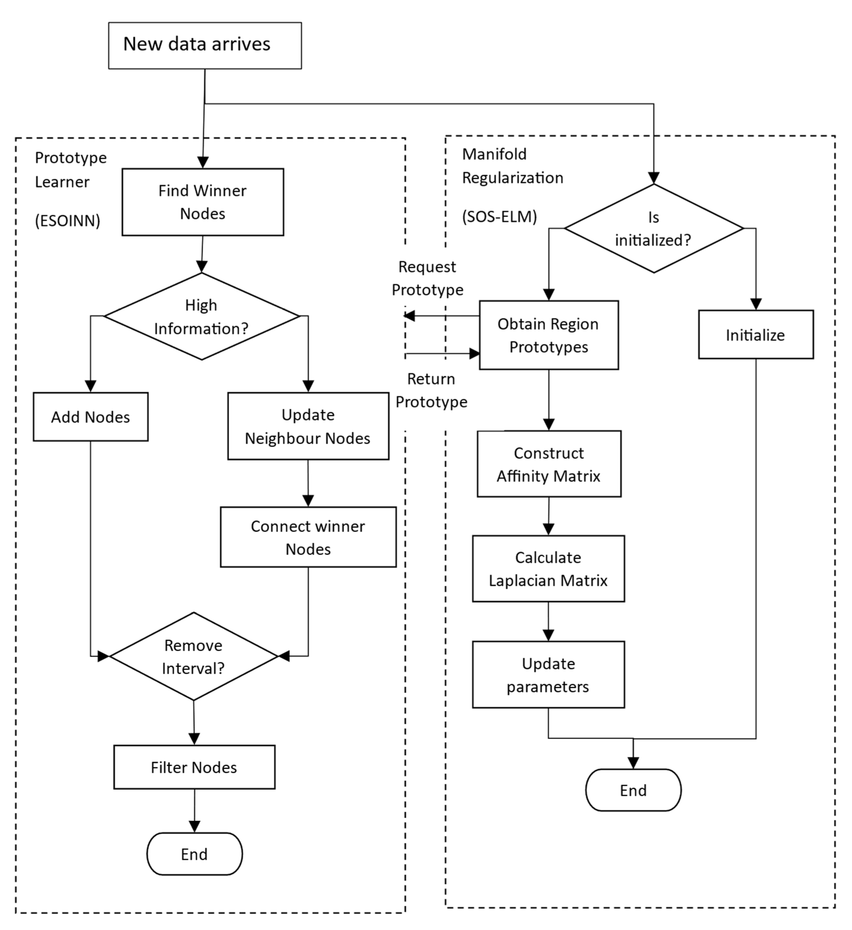
4. Proposed Approach
| Algorithm 2. Modified Enhanced Self-Organizing Incremental Neural Network (ESOINN) |
| Input: Labeled and Unlabeled Data set , maximum egde age , noise remove interval |
| Output: Set of Prototypes |
| 1: function train_esoinn (): |
| 2: foreach : |
| 3: if < 2: |
| 4: |
| 5: continue |
| 6: //find 1st winner |
| 7: //find 2nd winner |
| 8: if or : |
| 9: |
| 10: if (): |
| 11: |
| 12: else: |
| 13: if (): |
| 14: //assign label to the winner node |
| 15: |
| 16: . |
| 17: |
| 18: //if the label of the winners are the same or either winner has no label, connect the nodes |
| 19: if : |
| 20: |
| 21: else: |
| 22: |
| 23: |
| 24: for |
| 25: if or : |
| 26: |
| 27: if number of data is multiple of : |
| 28: foreach : |
| 29: if | |
| 30: //remove the node |
| 31: //only remove the unlabeled nodes |
| 32: else if and and : |
| 33: //remove node a |
| 34: else if and and : |
| 35: //remove node a |
| 36: end function |
| Algorithm 3. Prototype Regularized Semi-Supervised Online Extreme Learning Machine |
| Input: Labeled and Unlabeled Data set , maximum egde age , noise removes interval , Nearest Neighbors , Regularization Term , Hidden Layer Size . |
| 1: function train_esoinn (): |
| 2: //initialization phase |
| 3: Obtain the initial data set for initialization |
| 4: Process using Algorithm 2 to initialization ESOINN |
| 5: Use to calculate and using (16) and (17) respectively |
| 6: //sequential learning phase |
| 7: while (True): |
| 8: Obtain a partially labeled data set : |
| 9: Process using Algorithm 2 to update ESOINN |
| 10: obtain prototypes each for all data sets from the nodes in ESOINN |
| 11: Construct weight matrix using (21) |
| 12: Construct Laplacian matrix and penalty matrix |
| 13: Update hidden layer parameters using (19) |
| 14: Update using (20) |
| 15: end function |
5. Experiments
5.1. Experimental Setup
- (1)
- Sequential learning performance. This experiment was carried out to study how well this proposed approach learned the concept from sequential data, e.g., data stream. Since this proposed approach was designed to improve the practicality of manifold regularization for data stream mining, this experiment was divided into two types of experiments:
- This proposed approach versus the default RBF width parameter. This experiment compared how well this proposed approach compared with other benchmark approaches when the default width parameter was used. This experiment used , which is a popular default parameter in the documentation of machine learning algorithms that relies on the RBF kernel, e.g., support vector machines (SVM).
- This approach versus the optimum width parameter. This experiment was carried out to compare how this proposed approach compared when the width parameter was set to an optimum value to maximize the learning performance on the benchmark algorithm. This proposed approach was effective if it achieved the same or better performance compared to other approaches, as it indicates that this proposed approach could perform well even without the RBF kernel.
- (2)
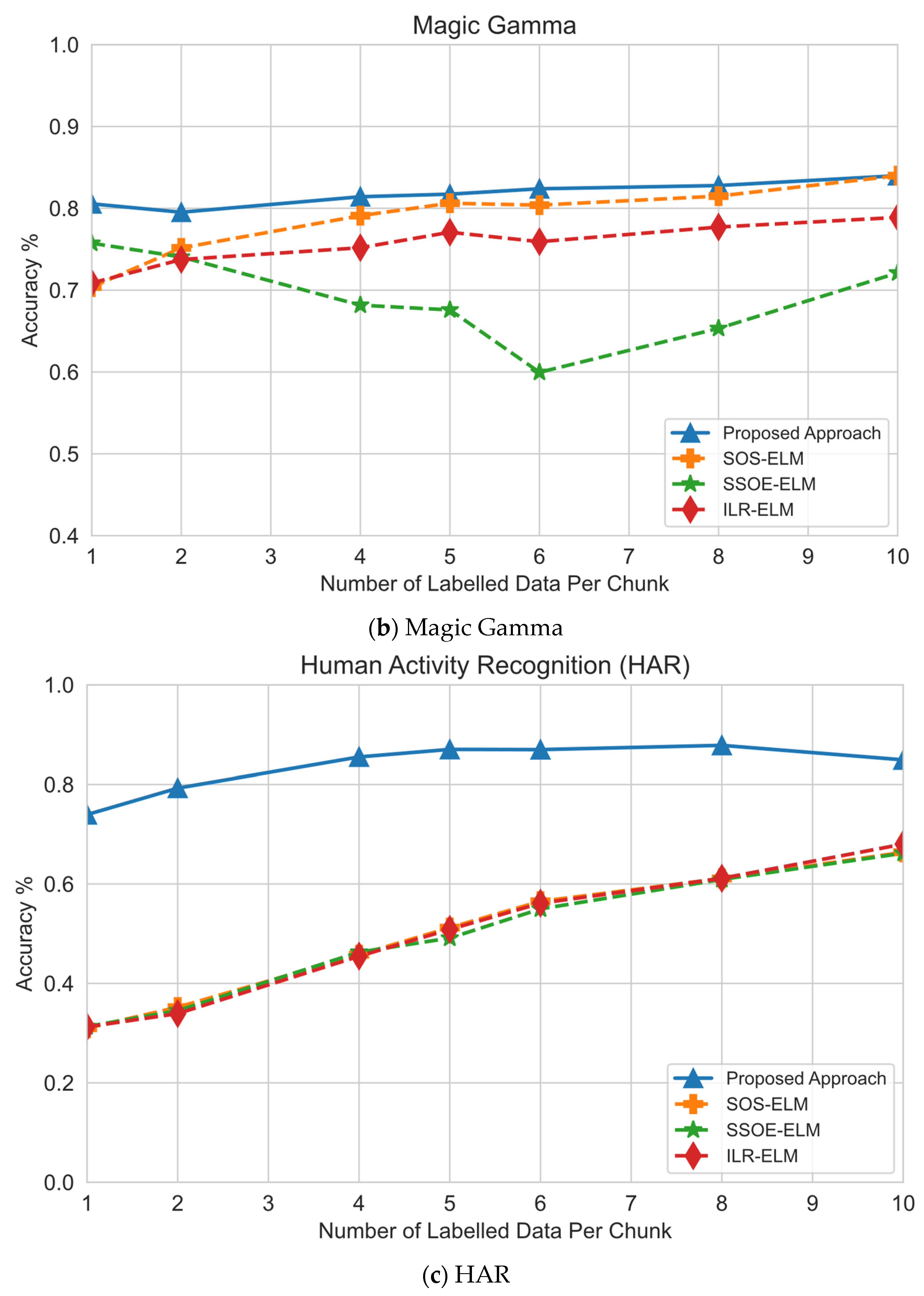
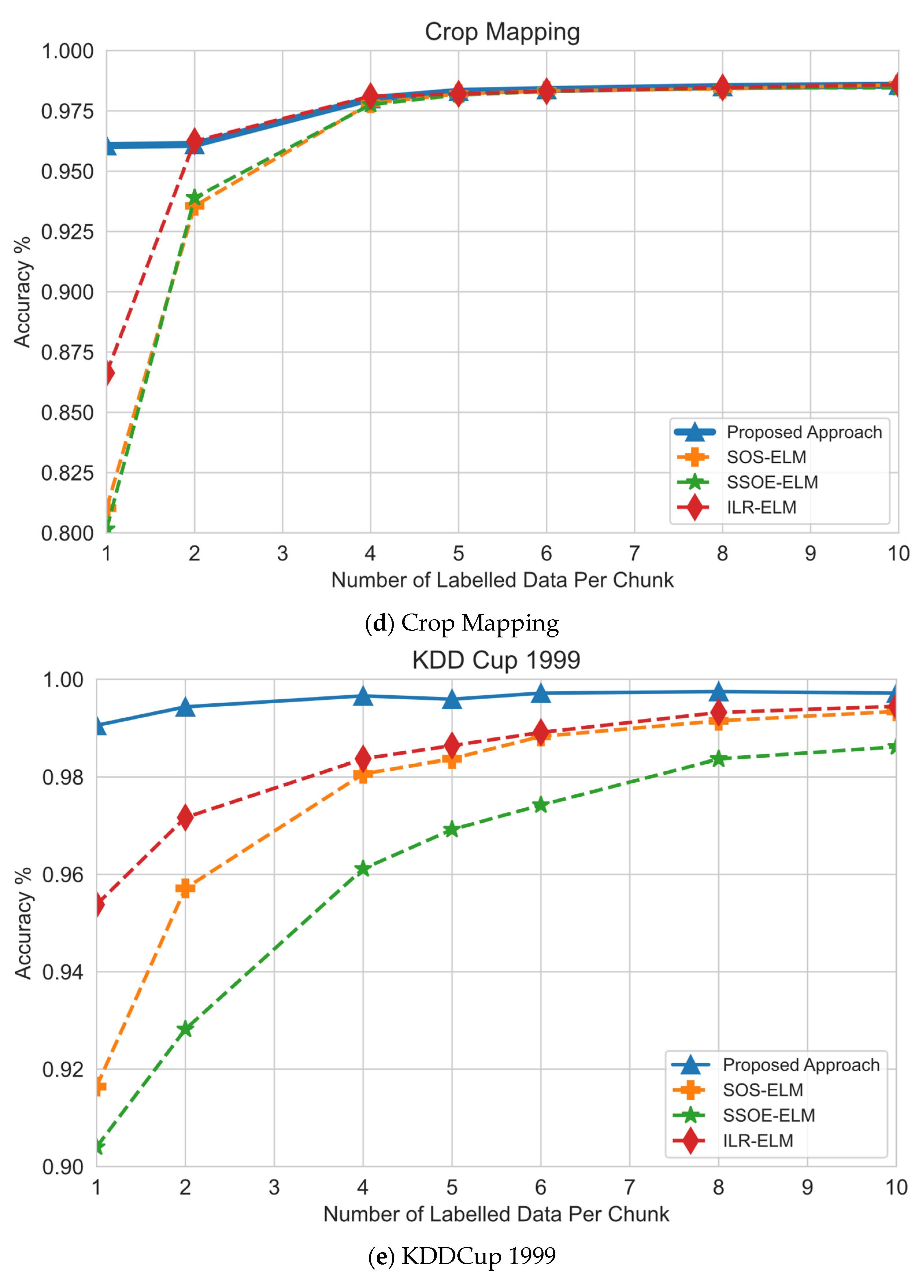
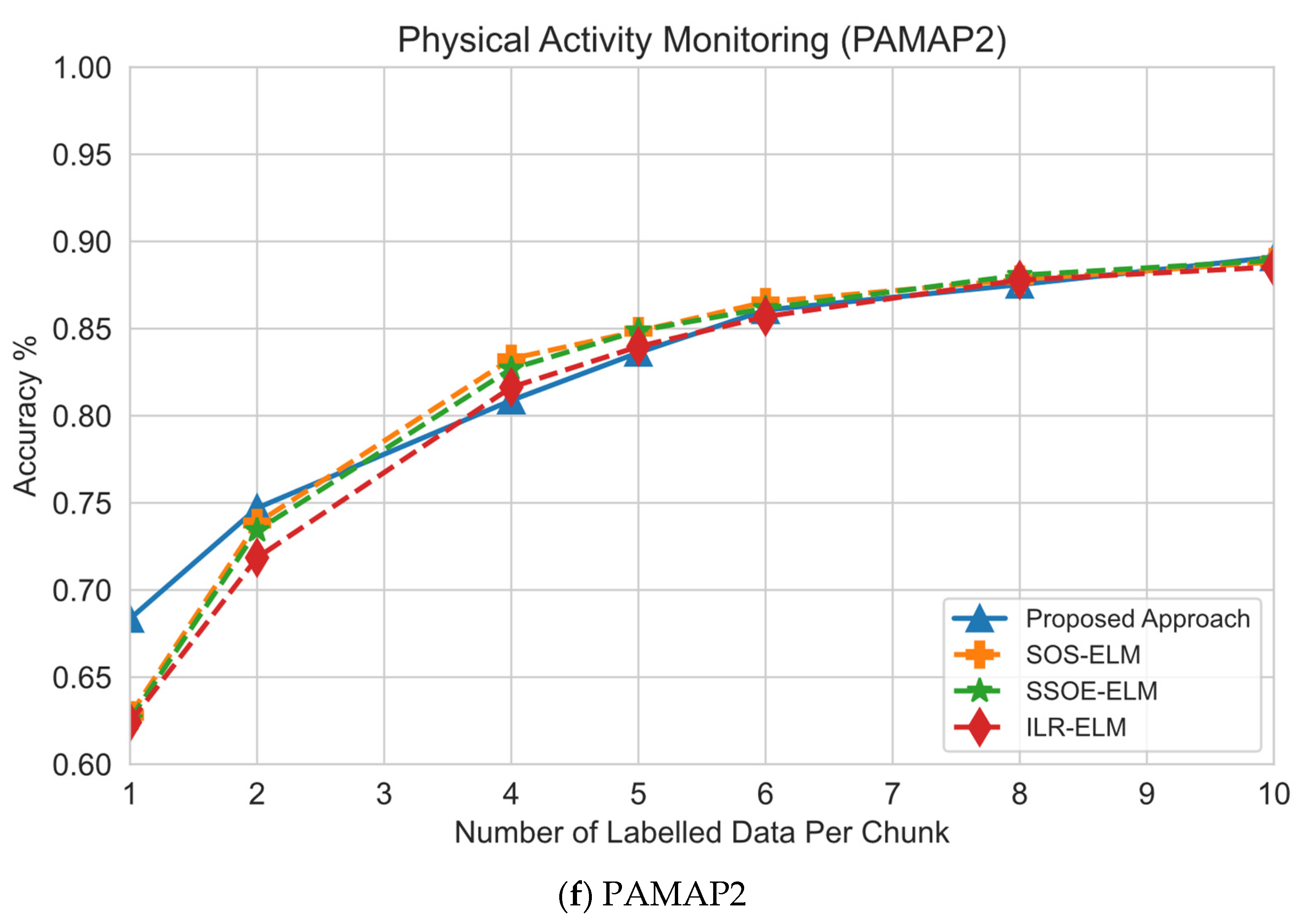
- Effect of the number of labeled samples and classification performance. This experiment was designed to understand the effect of the size of the labeled samples on classification performance.
- (3)
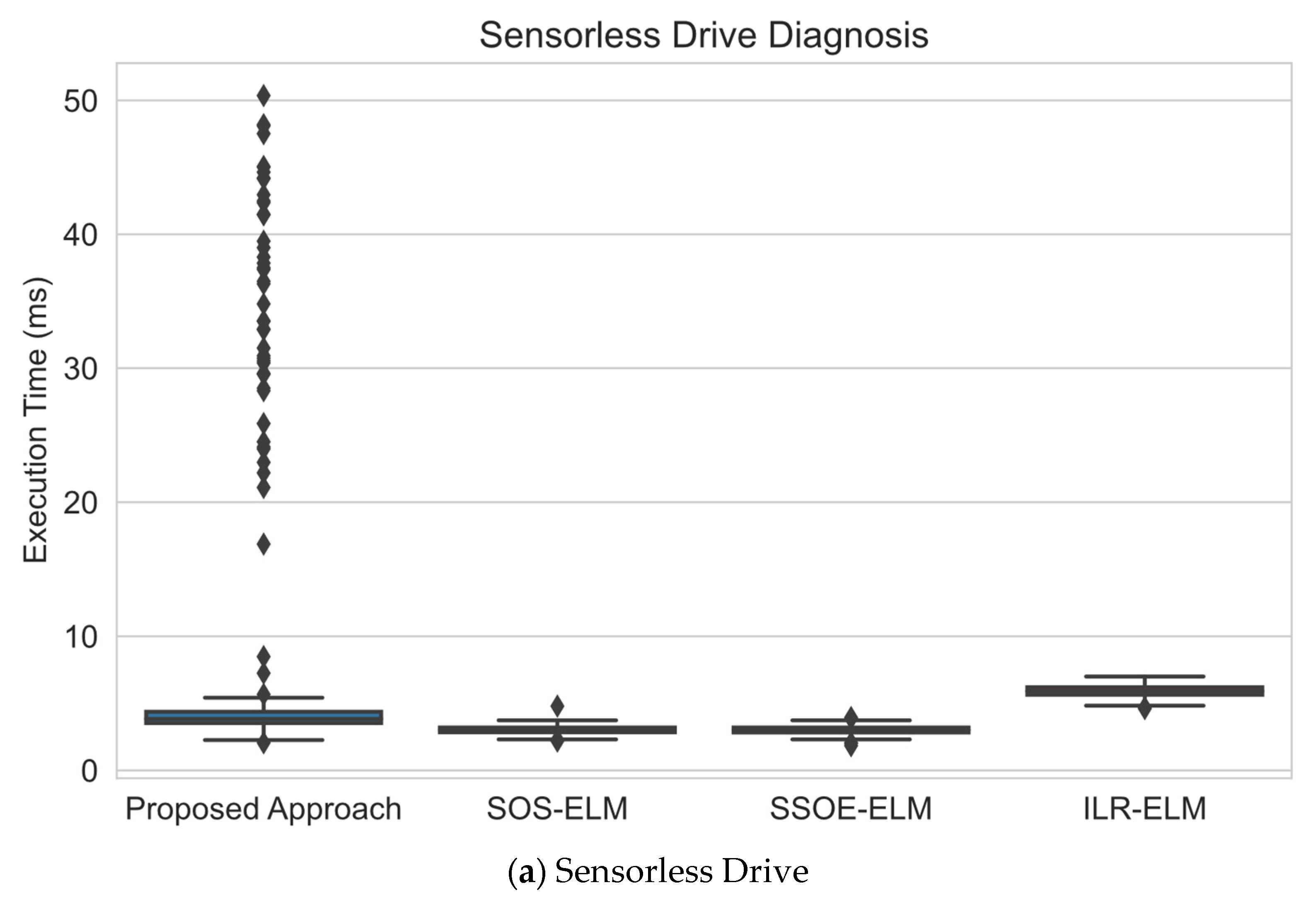
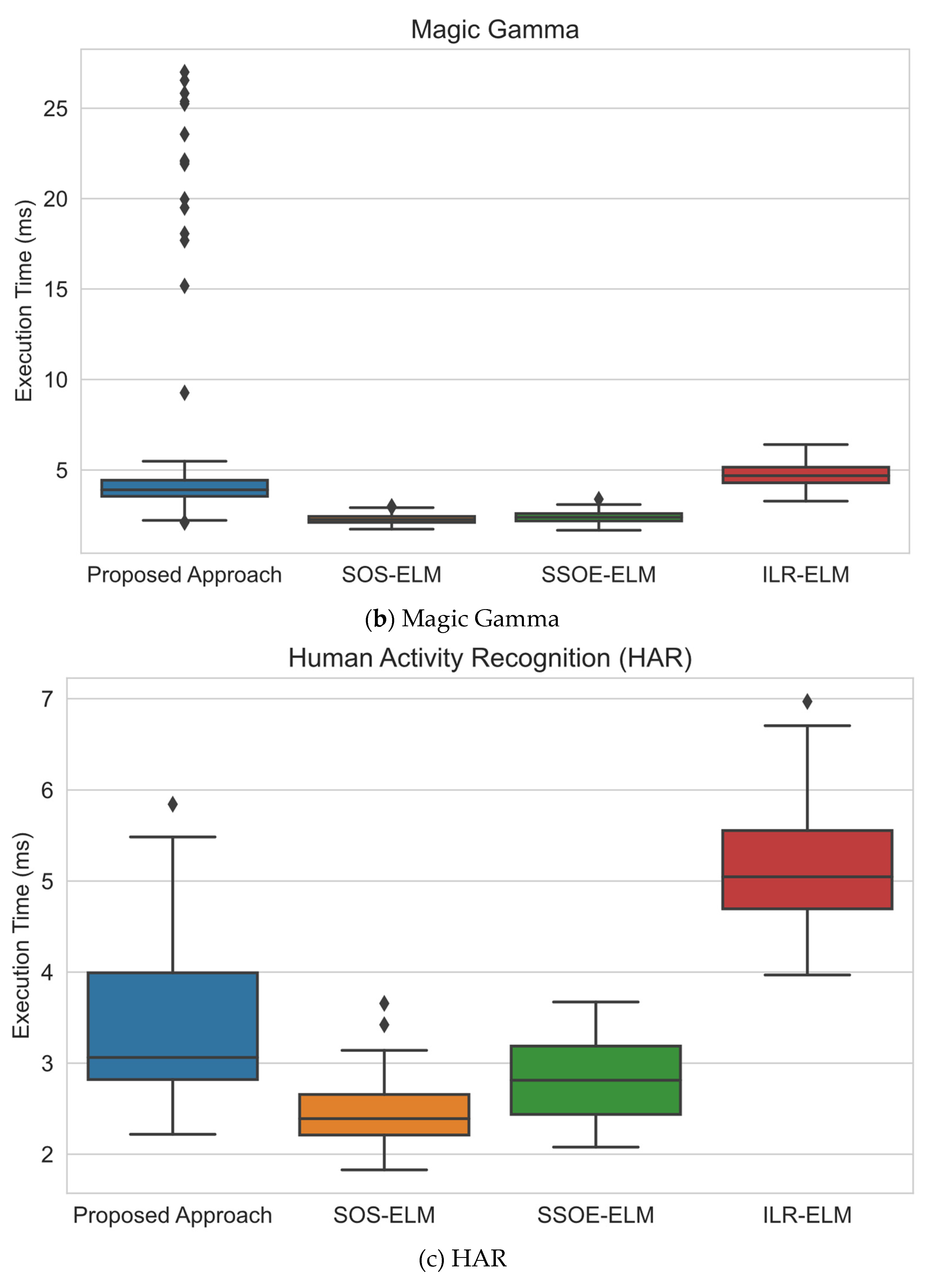
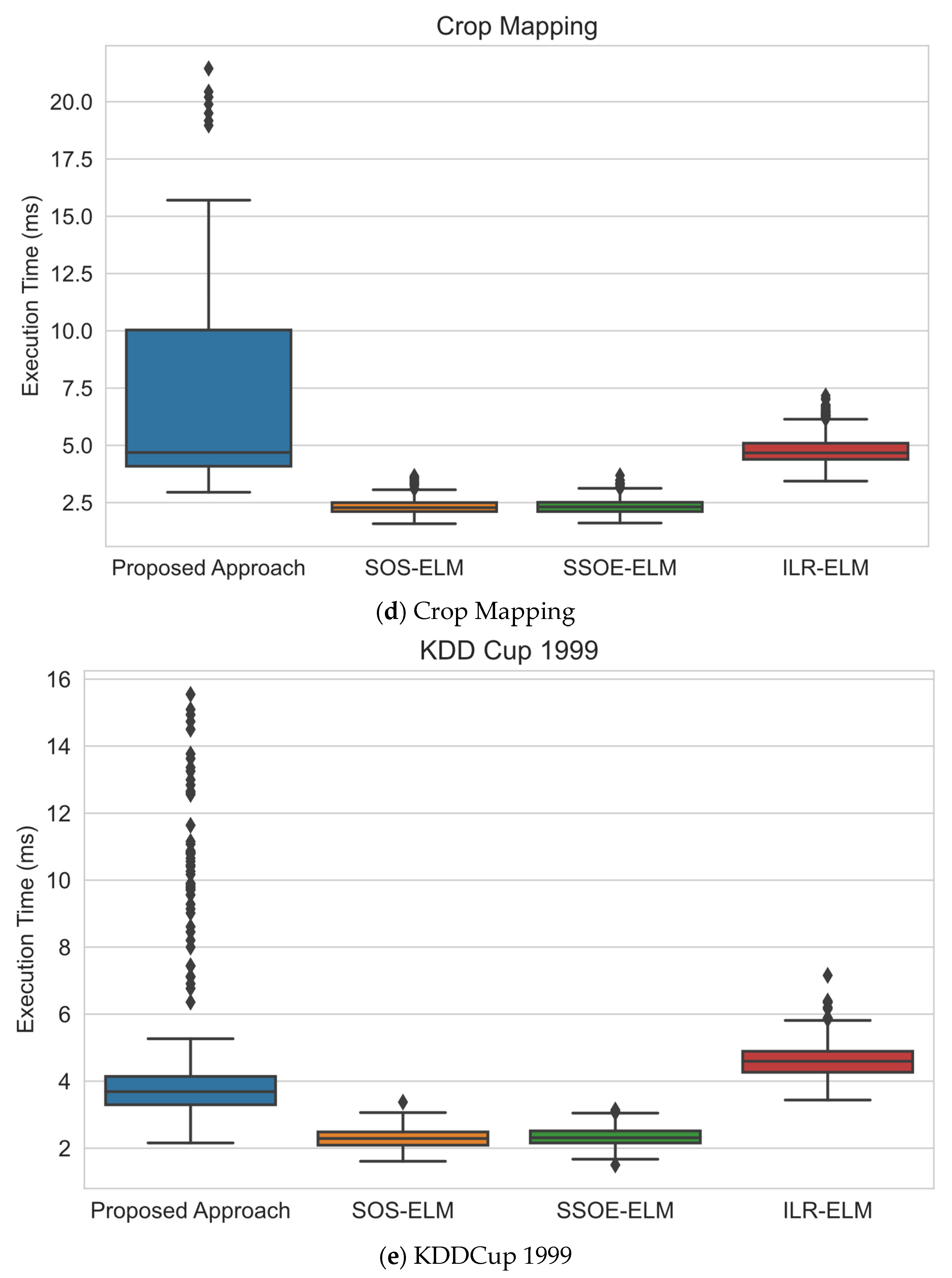
- Execution time analysis. As computational consumption is a major design consideration in applications such as data stream mining, this experiment was designed to study how long this proposed approach took to execute each update compared with other approaches.
5.2. Hyperparameter Selection
6. Results
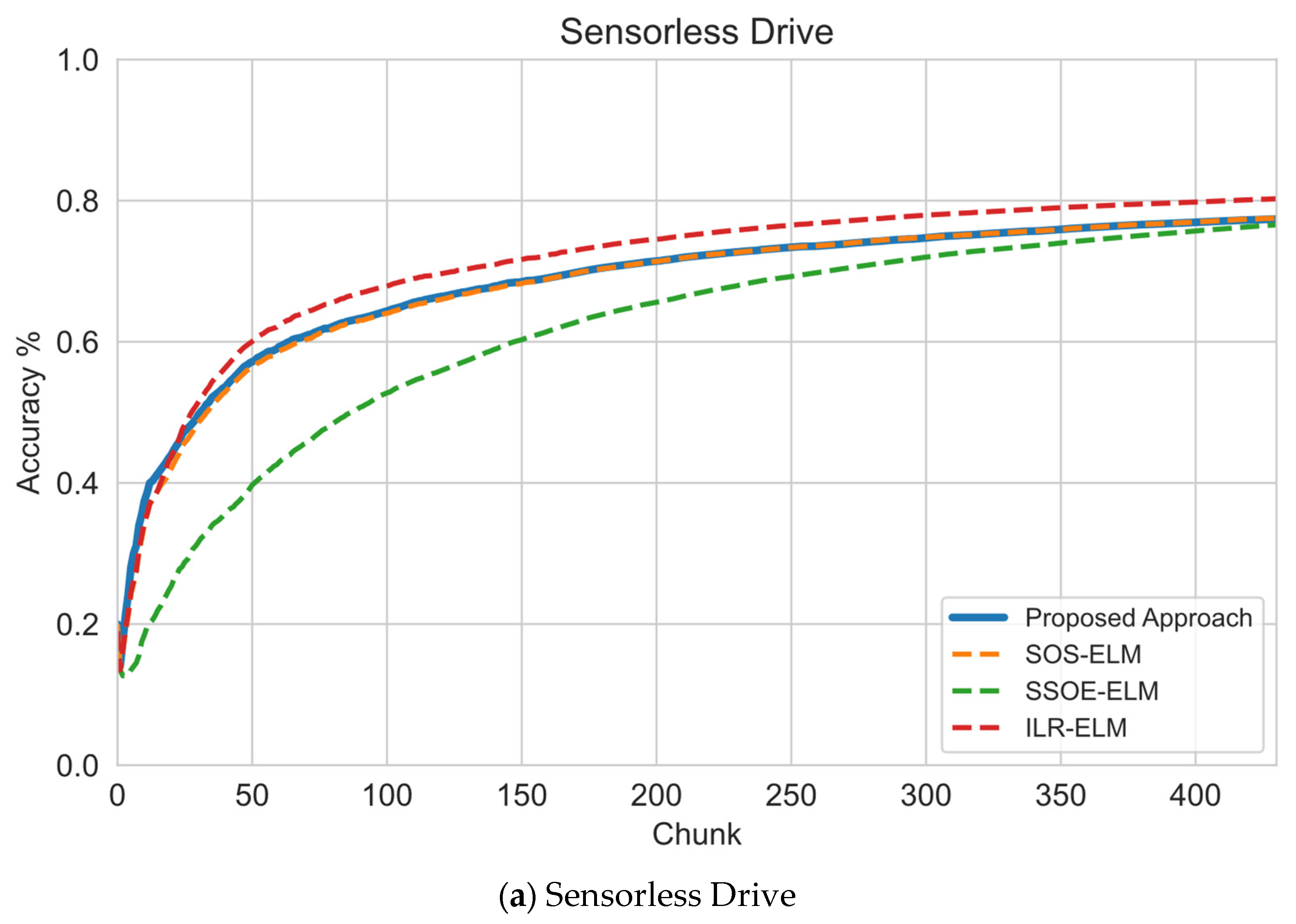
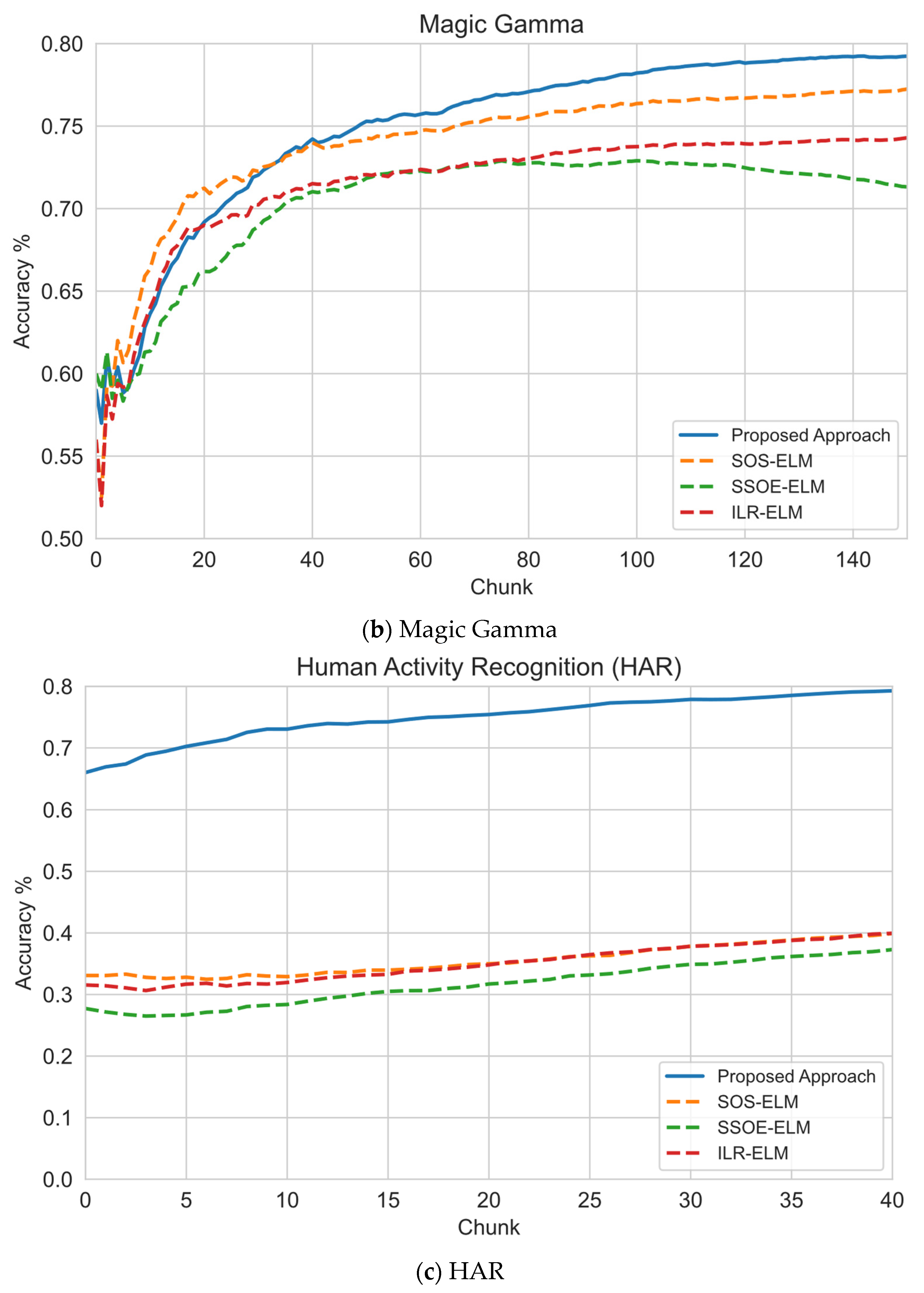
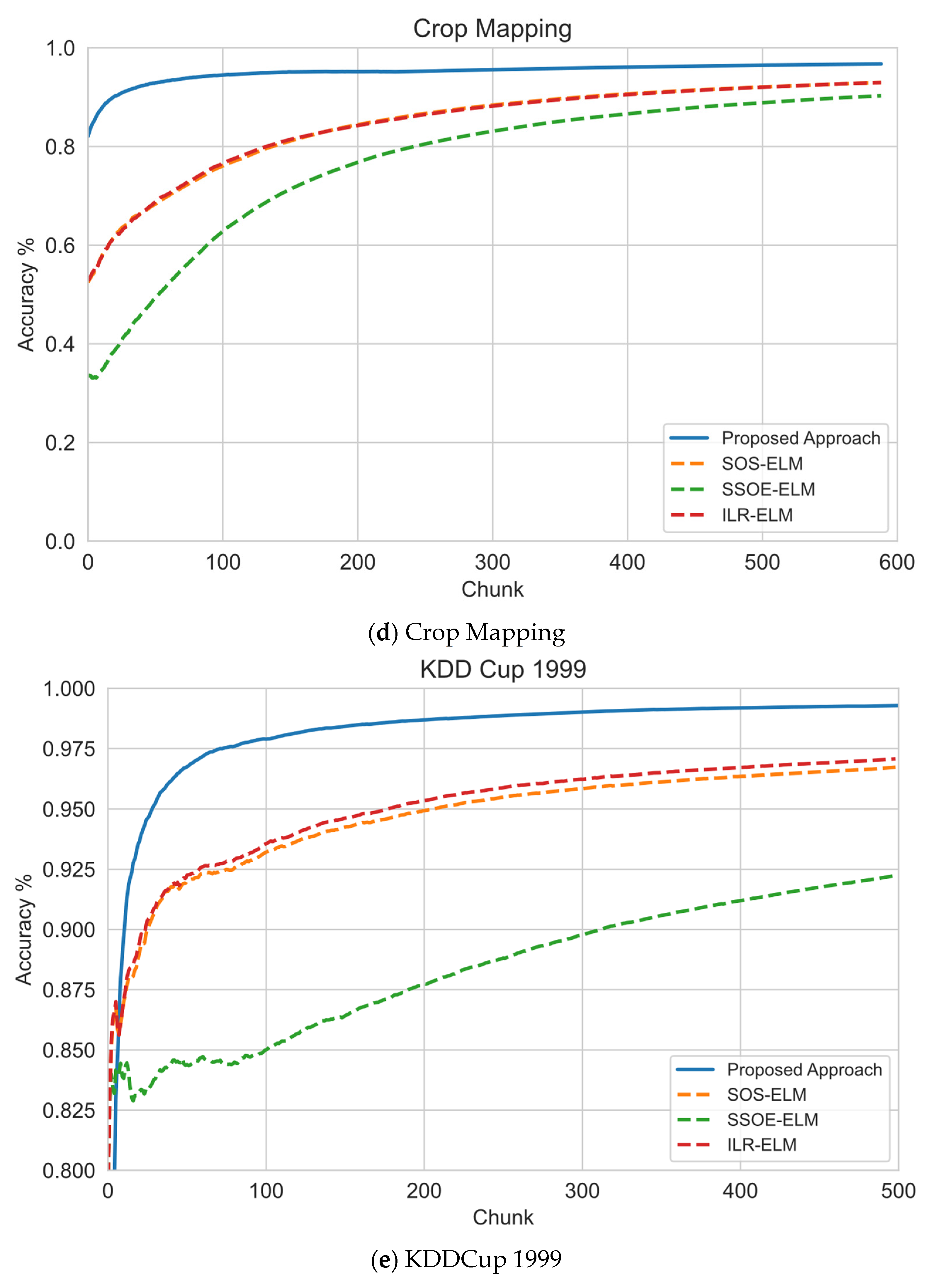
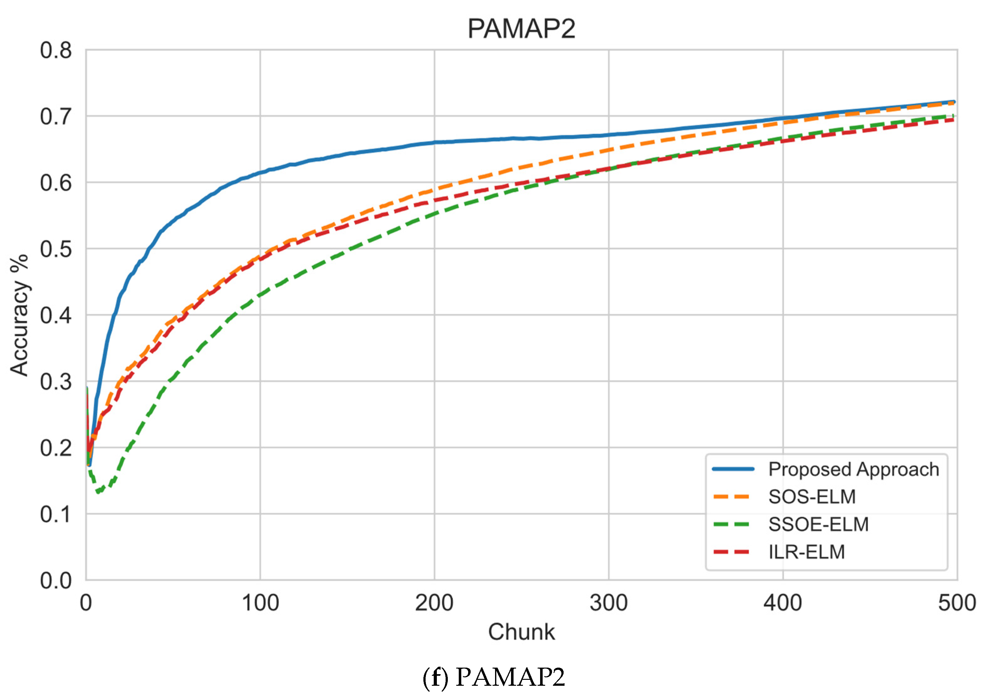
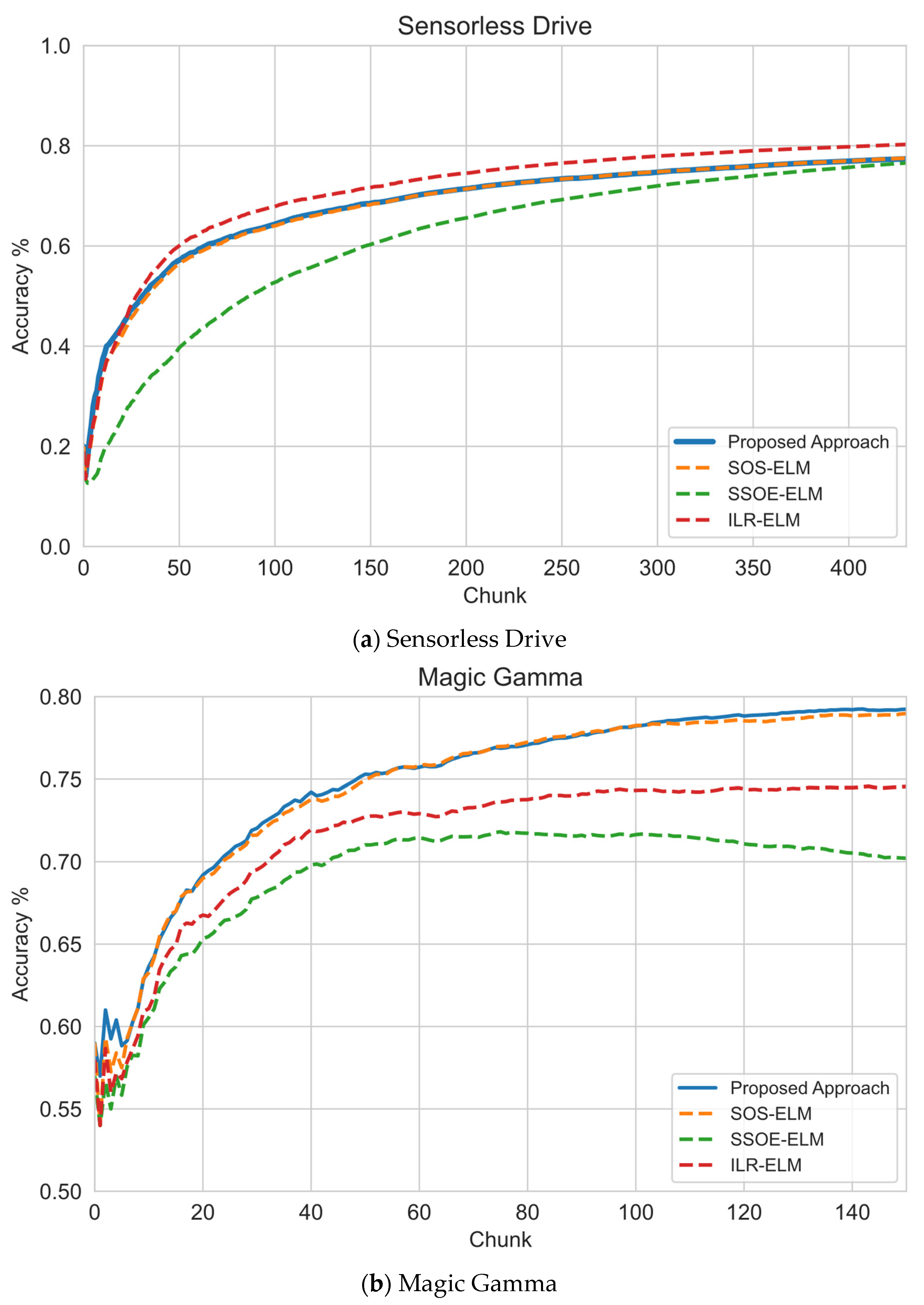
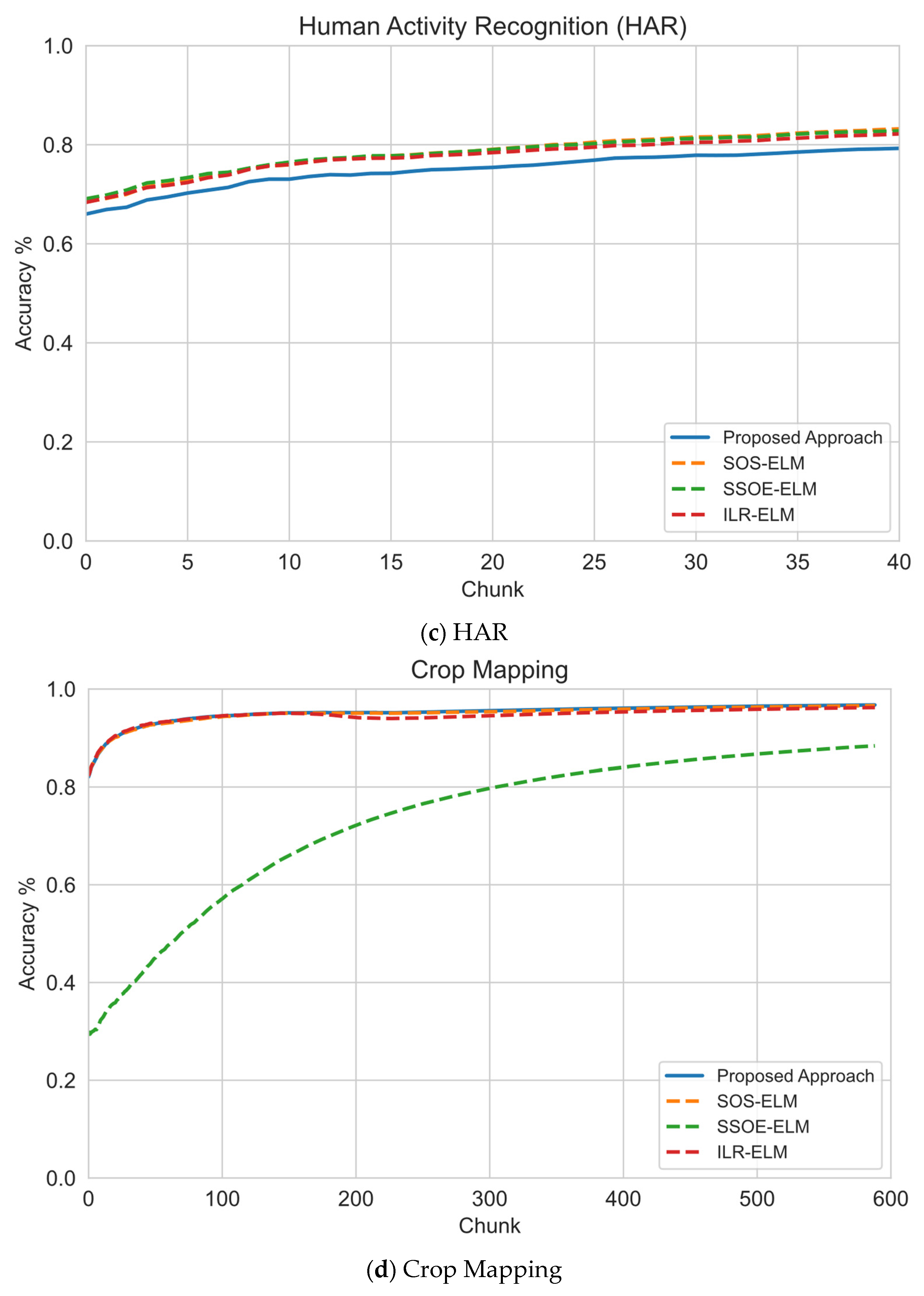
6.1. Sequential Learning Evaluation
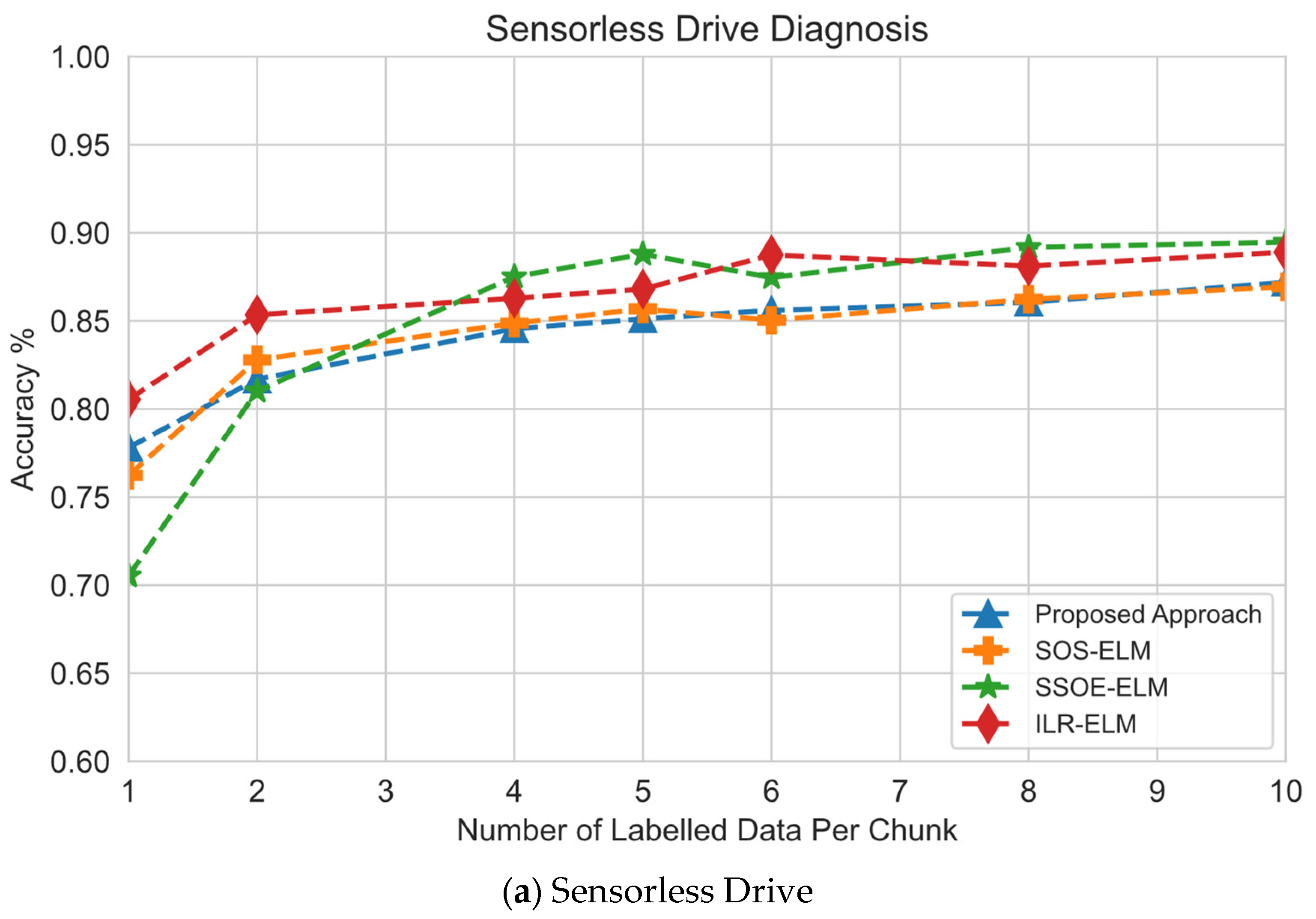
6.2. Effect of Number of Labeled Samples
6.3. Execution Time Analysis
7. Discussion
8. Conclusions
Author Contributions
Funding
Institutional Review Board Statement
Informed Consent Statement
Data Availability Statement
Acknowledgments
Conflicts of Interest
References
- Ramírez-Gallego, S.; Krawczyk, B.; García, S.; Woźniak, M.; Herrera, F. A Survey on Data Preprocessing for Data Stream Mining: Current Status and Future Directions. Neurocomputing 2017, 239, 39–57. [Google Scholar] [CrossRef]
- Domingos, P.; Hulten, G. Mining high-speed data streams. In Proceedings of the 6th ACM SIGKDD International Conference on Knowledge Discovery and Data Mining, Boston, MA, USA, 20–23 August 2000. [Google Scholar]
- Zhu, X.J. Semi-Supervised Learning Literature Survey; University of Wisconsin: Madison, WI, USA, 2005. [Google Scholar]
- Chapelle, O.; Bernhard, S.; Alexander, Z. Semi-Supervised Learning. IEEE Trans. Neural Netw. 2009, 20, 542. [Google Scholar] [CrossRef]
- Zhu, X.; Goldberg, A.B. Introduction to Semi-Supervised Learning. Synth. Lect. Artif. Intell. Mach. Learn. 2009, 3, 1–130. [Google Scholar] [CrossRef] [Green Version]
- Keogh, E.; Abdullah, M. Curse of dimensionality. In Encyclopedia of Machine Learning and Data Mining; Claude, S., Webb, G.I., Eds.; Springer: Boston, MA, USA, 2017; pp. 314–315. [Google Scholar]
- François, D.; Wertz, V.; Verleysen, M. The Concentration of Fractional Distances. IEEE Trans. Knowl. Data Eng. 2007, 19, 873–886. [Google Scholar] [CrossRef]
- Van Engelen, J.E.; Hoos, H.H. A Survey on Semi-Supervised Learning. Mach. Learn. 2020, 109, 373–440. [Google Scholar] [CrossRef] [Green Version]
- Belkin, M.; Niyogi, P.; Sindhwani, V. Manifold Regularization: A Geometric Framework for Learning from Labeled and Unlabeled Examples. J. Mach. Learn. Res. 2006, 7, 2399–2434. [Google Scholar]
- Huang, G.; Song, S.; Gupta, J.N.; Wu, C. Semi-Supervised and Unsupervised Extreme Learning Machines. IEEE Trans. Cybern. 2014, 44, 2405–2417. [Google Scholar] [CrossRef]
- Chapelle, O.; Sindhwani, V.; Keerthi, S.S. Optimization Techniques for Semi-Supervised Support Vector Machines. J. Mach. Learn. Res. 2008, 9, 203–233. [Google Scholar]
- Shen, Y.-Y.; Zhang, Y.-M.; Zhang, X.-Y.; Liu, C.-L. Online Semi-Supervised Learning with Learning Vector Quantization. Neurocomputing 2020, 399, 467–478. [Google Scholar] [CrossRef]
- Moh, Y.; Buhmann, J.M. Manifold Regularization for Semi-Supervised Sequential Learning. In Proceedings of the 2009 IEEE International Conference on Acoustics, Speech and Signal Processing, Washington, DC, USA, 19–24 April 2009. [Google Scholar]
- Kamiya, Y.; Ishii, T.; Furao, S.; Hasegawa, O. An Online Semi-Supervised Clustering Algorithm Based on a Self-Organizing Incremental Neural Network. In Proceedings of the 2007 International Joint Conference on Neural Networks, Orlando, FL, USA, 12–17 August 2007. [Google Scholar]
- Reynolds, D.A. Gaussian Mixture Models. Encycl. Biom. 2009, 741, 659–663. [Google Scholar]
- Quattoni, A.; Collins, M.; Darrell, T. Transfer learning for image classification with sparse prototype representations. In Proceedings of the 2008 IEEE Conference on Computer Vision and Pattern Recognition, Anchorage, AK, USA, 23–28 June 2008. [Google Scholar]
- Xue, W.; Wang, W. One-shot image classification by learning to restore prototypes. In Proceedings of the AAAI Conference on Artificial Intelligence, New York, NY, USA, 7–12 February 2020. [Google Scholar]
- Tran, M.Q.; Elsisi, M.; Liu, M.K. Effective Feature Selection with Fuzzy Entropy and Similarity Classifier for Chatter Vibration Diagnosis. Measurement 2021, 184, 109962. [Google Scholar] [CrossRef]
- Furao, S.; Ogura, T.; Hasegawa, O. An Enhanced Self-Organizing Incremental Neural Network for Online Unsupervised Learning. Neural Netw. 2007, 20, 893–903. [Google Scholar] [CrossRef] [PubMed]
- Jia, X.; Wang, R.; Liu, J.; Powers, D.M. A Semi-Supervised Online Sequential Extreme Learning Machine Method. Neurocomputing 2016, 174, 168–178. [Google Scholar] [CrossRef]
- Niyogi, P. Manifold Regularization and Semi-Supervised Learning: Some Theoretical Analyses. J. Mach. Learn. Res. 2013, 14, 1229–1250. [Google Scholar]
- Melacci, S.; Belkin, M. Laplacian Support Vector Machines Trained in the Primal. J. Mach. Learn. Res. 2011, 12, 1149–1184. [Google Scholar]
- Goldberg, A.B.; Li, M.; Zhu, X. Online manifold regularization: A new learning setting and empirical study. In Proceedings of the Joint European Conference on Machine Learning and Knowledge Discovery in Databases, Antwerp, Belgium, 14–18 September 2008. [Google Scholar]
- Liu, Y.; Xu, Z.; Li, C. Distributed Online Semi-Supervised Support Vector Machine. Inf. Sci. 2018, 466, 236–357. [Google Scholar] [CrossRef]
- Scardapane, S.; Fierimonte, R.; di Lorenzo, P.; Panella, M.; Uncini, A. Distributed Semi-Supervised Support Vector Machines. Neural Netw. 2016, 80, 43–52. [Google Scholar] [CrossRef]
- Yang, L.; Yang, S.; Li, S.; Liu, Z.; Jiao, L. Incremental Laplacian Regularization Extreme Learning Machine for Online Learning. Appl. Soft Comput. 2017, 59, 546–555. [Google Scholar] [CrossRef]
- Da Silva, C.A.; Krohling, R.A. Semi-supervised online elastic extreme learning machine for data classification. In Proceedings of the 2018 International Joint Conference on Neural Networks (IJCNN), Rio de Janeiro, Brazil, 8–13 July 2018. [Google Scholar]
- Likas, A.; Vlassis, N.; Verbeek, J.J. The Global K-Means Clustering Algorithm. Pattern Recognit. 2003, 36, 451–461. [Google Scholar] [CrossRef] [Green Version]
- Fritzke, B. A Growing Neural Gas Network Learns Topologies. Adv. Neural Inf. Proces. Syst. 1995, 7, 625–632. [Google Scholar]
- Kohonen, T. The Self-Organizing Map. Proc. IEEE 1990, 78, 1464–1480. [Google Scholar] [CrossRef]
- Furao, S.; Hasegawa, O. An Incremental Network for on-Line Unsupervised Classification and Topology Learning. Neural Netw. 2006, 19, 90–106. [Google Scholar] [CrossRef] [PubMed]
- Huang, G.-B.; Zhu, Q.-Y.; Siew, C.-K. Extreme Learning Machine: Theory and Applications. Neurocomputing 2006, 70, 489–501. [Google Scholar] [CrossRef]
- Zhang, R.; Lan, Y.; Huang, G.B.; Xu, Z.B. Universal Approximation of Extreme Learning Machine with Adaptive Growth of Hidden Nodes. IEEE Trans. Neural Netw. Learn. Syst. 2012, 23, 365–371. [Google Scholar] [CrossRef]
- Albadra, M.A.A.; Tiuna, S. Extreme Learning Machine: A Review. Int. J. Appl. Eng. Res. 2017, 12, 4610–4623. [Google Scholar]
- Lin, B.; He, X.; Ye, J. A Geometric Viewpoint of Manifold Learning. Appl. Inform. 2015, 2, 3. [Google Scholar] [CrossRef] [Green Version]
- Gama, J.; Sebastião, R.; Rodrigues, P.P. On Evaluating Stream Learning Algorithms. Mach. Learn. 2012, 90, 1–30. [Google Scholar] [CrossRef] [Green Version]
- Hochreiter, S. The Vanishing Gradient Problem During Learning Recurrent Neural Nets and Problem Solutions. Int. J. Uncertain. Fuzziness Knowl.-Based Syst. 1998, 6, 107–116. [Google Scholar] [CrossRef] [Green Version]


| Data Set | #Samples | #Features | #Classes | #Training Samples | #Test Samples | #Training Steps | #Labeled Samples | Data Characteristics |
|---|---|---|---|---|---|---|---|---|
| Sensorless Drive | 58,509 | 49 | 11 | 46,807 | 11,701 | 469 | 2340 | High-Dimensional |
| Magic Gamma | 19,020 | 11 | 11 | 15,216 | 3804 | 152 | 760 | Noisy/Class Imbalance |
| Human Activity Recognition (HAR) | 10,299 | 561 | 6 | 5881 | 4418 | 58 | 290 | Noisy/High-Dimensional |
| Crop Mapping | 325,834 | 175 | 7 | 60,000 | 65,167 | 600 | 3000 | High-Dimensional |
| KDDCup 1999 | 494,021 | 42 | 12 | 50,000 | 98,805 | 500 | 2500 | Class Imbalance |
| Physical Activity Monitoring (PAMAP2) | 1,942,872 | 52 | 12 | 50,000 | 388,575 | 500 | 2500 | Noisy/High-Dimensional |
| Data Set | |||
|---|---|---|---|
| Crop Mapping | 0.001 | 0.00001 | 1 |
| HAR | 10 | 0.001 | |
| KDDCup1999 | 20 | 0.00001 | 1 |
| Magic Gamma | 1 | 0.00001 | 1 |
| PAMAP2 | 10 | 0.00001 | 1 |
| Sensorless Drive | 0.01 | 0.00001 | 1 |
| Data Set | Number of Labels | This Proposed Approach | SOS-ELM | SSOE-ELM | ILR-ELM | OS-ELM | RSLVQ |
|---|---|---|---|---|---|---|---|
| Crop Mapping | 1 | 96.06 | 81.03 | 80.16 | 86.63 | 83.29 | 88.43 |
| 5 | 98.31 | 98.2 | 98.16 | 98.2 | 82.54 | 88.43 | |
| 10 | 98.56 | 98.58 | 98.45 | 98.58 | 83.88 | 88.43 | |
| Average Accuracy | 97.64 | 92.60 | 92.26 | 94.47 | 83.24 | 88.43 | |
| Average Ranking | 1 | 3 | 4 | 2 | 6 | 5 | |
| HAR | 1 | 73.95 | 30.99 | 31.33 | 31.26 | 70.96 | 81.37 |
| 5 | 87.01 | 51.22 | 49.12 | 50.86 | 70.94 | 81.37 | |
| 10 | 84.9 | 66.39 | 66.18 | 68.02 | 71 | 81.37 | |
| Average Accuracy | 81.95 | 49.53 | 48.88 | 50.05 | 70.97 | 81.37 | |
| Average Ranking | 1 | 5 | 6 | 4 | 3 | 2 | |
| KDDCup 1999 | 1 | 99.05 | 91.64 | 90.4 | 68.02 | 18.3 | 98.1 |
| 5 | 99.59 | 98.37 | 96.92 | 98.64 | 87.8 | 98.1 | |
| 10 | 99.72 | 99.34 | 98.61 | 99.45 | 78.35 | 98.1 | |
| Average Accuracy | 99.45 | 96.45 | 95.31 | 88.70 | 61.48 | 98.10 | |
| Average Ranking | 1 | 3 | 4 | 5 | 6 | 2 | |
| Magic Gamma | 1 | 80.55 | 70.37 | 75.74 | 70.87 | 69.14 | 79.34 |
| 5 | 81.73 | 80.63 | 67.59 | 77.08 | 66.93 | 79.34 | |
| 10 | 83.99 | 82.6 | 72.11 | 78.89 | 69.77 | 79.34 | |
| Average Accuracy | 82.09 | 77.87 | 71.81 | 75.61 | 68.61 | 79.34 | |
| Average Ranking | 1 | 3 | 5 | 4 | 6 | 2 | |
| PAMAP2 | 1 | 68.35 | 62.81 | 62.57 | 62.41 | 4.2 | 62.54 |
| 5 | 83.62 | 84.86 | 84.87 | 83.97 | 30.26 | 62.54 | |
| 10 | 89.1 | 88.82 | 88.91 | 88.53 | 29.52 | 62.54 | |
| Average Accuracy | 80.36 | 78.83 | 78.78 | 78.30 | 21.33 | 62.54 | |
| Average Ranking | 1 | 2 | 3 | 4 | 6 | 5 | |
| Sensorless Drive | 1 | 77.82 | 76.23 | 70.53 | 80.54 | 48.46 | 81.27 |
| 5 | 85.11 | 85.68 | 88.79 | 86.81 | 46.1 | 81.27 | |
| 10 | 87.19 | 86.93 | 89.47 | 88.9 | 43.16 | 81.27 | |
| Average Accuracy | 83.37 | 82.95 | 82.93 | 85.42 | 45.91 | 81.27 | |
| Average Ranking | 2 | 3 | 4 | 1 | 6 | 5 | |
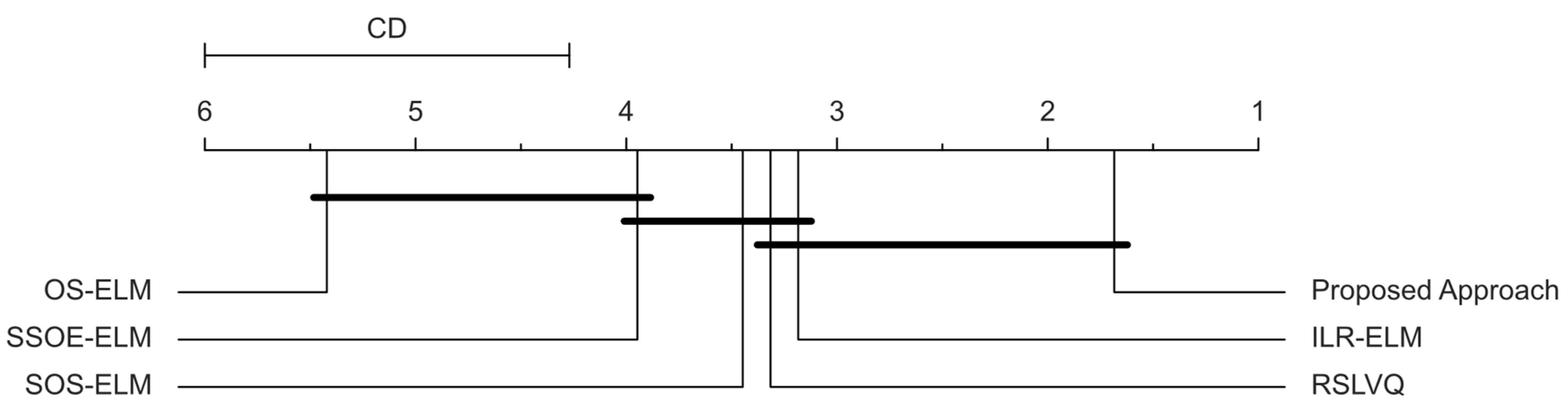
| Overall Average Accuracy | 87.48 | 79.7 | 78.33 | 78.76 | 58.59 | 81.84 | |
| Overall Ranking | 1.72 | 3.36 | 3.83 | 3.31 | 5.39 | 3.39 |
Publisher’s Note: MDPI stays neutral with regard to jurisdictional claims in published maps and institutional affiliations. |
© 2022 by the authors. Licensee MDPI, Basel, Switzerland. This article is an open access article distributed under the terms and conditions of the Creative Commons Attribution (CC BY) license (https://creativecommons.org/licenses/by/4.0/).
Share and Cite
Muhammad Zaly Shah, M.Z.; Zainal, A.; Ghaleb, F.A.; Al-Qarafi, A.; Saeed, F. Prototype Regularized Manifold Regularization Technique for Semi-Supervised Online Extreme Learning Machine. Sensors 2022, 22, 3113. https://doi.org/10.3390/s22093113
Muhammad Zaly Shah MZ, Zainal A, Ghaleb FA, Al-Qarafi A, Saeed F. Prototype Regularized Manifold Regularization Technique for Semi-Supervised Online Extreme Learning Machine. Sensors. 2022; 22(9):3113. https://doi.org/10.3390/s22093113
Chicago/Turabian StyleMuhammad Zaly Shah, Muhammad Zafran, Anazida Zainal, Fuad A. Ghaleb, Abdulrahman Al-Qarafi, and Faisal Saeed. 2022. "Prototype Regularized Manifold Regularization Technique for Semi-Supervised Online Extreme Learning Machine" Sensors 22, no. 9: 3113. https://doi.org/10.3390/s22093113