
Exploration-Based SLAM (e-SLAM) for the Indoor Mobile Robot Using Lidar


1
Department of Mechanical Engineering, National Yang Ming Chiao Tung University, Hsinchu 30010, Taiwan
2
Department of Mechanical Engineering, Chung Hua University, Hsinchu 30012, Taiwan
*
Author to whom correspondence should be addressed.
Sensors 2022, 22(4), 1689; https://doi.org/10.3390/s22041689
Submission received: 27 January 2022
/
Revised: 16 February 2022
/
Accepted: 18 February 2022
/
Published: 21 February 2022
(This article belongs to the Special Issue Advanced Sensing Techniques for Autonomous Vehicles and Advanced Driver Assistance Systems (ADAS))
Abstract
:This paper attempts to uncover one possible method for the IMR (indoor mobile robot) to perform indoor exploration associated with SLAM (simultaneous localization and mapping) using LiDAR. Specifically, the IMR is required to construct a map when it has landed on an unexplored floor of a building. We had implemented the e-SLAM (exploration-based SLAM) using the coordinate transformation and the navigation prediction techniques to achieve that purpose in the engineering school building which consists of many 100-m2 labs, corridors, elevator waiting space and the lobby. We first derive the LiDAR mesh for the orthogonal walls and filter out the static furniture and dynamic humans in the same space as the IMR. Then, we define the LiDAR pose frame including the translation and rotation from the orthogonal walls. According to the MSC (most significant corner) obtained from the intersection of the orthogonal walls, we calculate the displacement of the IMR. The orientation of the IMR is calculated from the alignment of orthogonal walls in the consecutive LiDAR pose frames, which is also assisted by the LQE (linear quadratic estimation) method. All the computation can be done in a single processor machine in real-time. The e-SLAM technique leads to a potential for the in-house service robot to start operation without having pre-scan LiDAR maps, which can save the installation time of the service robot. In this study, we use only the LiDAR and compared our result with the IMU to verify the consistency between the two navigation sensors in the experiments. The scenario of the experiment consists of rooms, corridors, elevators, and the lobby, which is common to most office buildings.
1. Introduction
Navigation is the basic function of autonomous vehicles in daily and industrial applications. For outdoor environment, vehicle localization and navigation can be achieved with the assistance of global positioning systems (GPS). However, in the indoor environment, the traditional navigation technology will fail due to the lack of satellite positioning signals [1]. Vehicle cruising in the indoor space can be localized and navigated through some characteristic graphics or marked points if there is a premade map of the space. If it is moving in an unknown environment, the localization and mapping must be carried out simultaneously. However, accurate localization requires an accurate map and vice versa. The localization and mapping must be concurrently performed which creates a complex problem called simultaneous localization and mapping (SLAM) first proposed by Hugh Durrant-Whyte and John J. Leonard [2,3,4].
Sensors are the way robots or self-driving vehicles perceive their environments. The selection and installation of sensors determine the specific form of observation results, and also affect the difficulty of SLAM problems. According to the major sensor, simultaneous localization and mapping can be divided into Visual-SLAM and LiDAR-SLAM.
Visual SLAM uses the vision camera as the major sensor to find features in the image and then use these features to match the known image for localization. Inspired by human vision, some studies use stereo cameras to perform SLAM [5,6,7,8]. In addition, monocular cameras can construct SLAM [9,10], including feature description methods [11,12], LSD-SLAM [13] and SVO [14]. An effective Visual SLAM needs to extract and match features, which requires huge amounts of calculations and is time-consuming for modern computers. The relationship between the image coordinates of the matching points and the space coordinates is nonlinear. Matching these features will introduce many constraints that make the process of the optimization problem of multiple variables more complicated and slower. These two difficulties make the Visual SLAM system still a very challenging task. In addition, the vision camera cannot extract features from textureless regions, which also limits the use of Visual SLAM. LiDAR SLAM mainly uses LiDAR for sensing environments. The relative movement and pose change of the laser radar can be determined by matching and comparison of the point clouds at different times. Its advantages are stability, simple, accurate map information and less calculation than Visual SLAM. It has been widely used, most of which use iterative closest point (ICP) [15,16,17,18] scan-matching technique, including Scan to Scan [19,20,21,22,23] and Scan to Map [24,25,26,27]. For the comparison of various LiDAR-based SLAMs, please refer to the literature [28].
The most important core of solving the problem of SLAM is finding the motion and observation models to provide efficient and consistent calculations for estimation and measurement updates. However, due to the presence of noise in the measurement, the subsequent estimation will transmit the noise error. The calculation algorithm of SLAM can be roughly divided into two categories: filters and optimization methods. The filter methods are based on two kinds: Gaussian filter (GF) and particle filter (PF). The Gaussian filters including Kalman filter (KF) and extended Kalman filter (EKF) separately deal with linear and nonlinear issues. The optimization method commonly uses pose graph optimization to minimize the square errors to solve the SLAM. In addition, since artificial intelligence (AI) has prevailed in recent years, learning methods are also used to solve the SLAM problem [29,30,31,32].
The principle of the Kalman filter is to use the current state information and input to infer the output at the next moment. Assuming that the noise follows a Gaussian distribution, the recursive algorithm is used to effectively estimate the pose of the vehicle. If the error model is a Gaussian distribution, the accuracy of the estimated result will be quite good. The advantage of the Kaman filter lies in its fast convergence. The disadvantage is that the error model must be a Gaussian distribution as otherwise the estimated result will lack accuracy. Besides, the size of the state vectors directly affects the dimension and time of the matrix operation. The SLAM based on the Kalman filter assumes that the system is linear, but in fact, the problem of SLAM is rarely linear. Therefore, the Extended Kalman filter (EKF) was developed to solve the nonlinear positioning problem. The EKF-SLAM was first proposed by Smith et al. [33], after which many researchers further improved this method [34,35,36].
The particle filter SLAM [24,37,38] is a recursive filter using a Monte Carlo algorithm to estimate the pose and movement path of the vehicle. Random distribution of particles is sampled. Each particle in the sample represents the vehicle trajectory and a map. These particles are weighted to fit a closer actual environment, and re-sampling is performed according to the distribution result. As the robot continues to move in space, particles will gradually gather at the most likely pose of the robot in space, and the map will be updated simultaneously. Although the particle filter algorithm can be used as an effective method to solve the SLAM problem, the main problem is that a large number of samples are required to approximate the posterior probability density of the system. The more complex environment the robot faces, the more samples are needed to describe the posterior probability and the higher the complexity of the algorithm.
In addition to solving SLAM problems with filters, graph-based SLAM [39,40,41] takes a different approach for estimating a robot trajectory. It creates a pose graph, whose node corresponds to a pose of the robot during mapping and every edge between two nodes corresponds to a spatial constraint between them. The bundle adjustment is performed to estimate trajectory and map from the input feature tracks. Cartographer is a Google open-source project developed in 2016. It is a system that provides 2D and 3D real-time SLAM under multiple platforms and sensor configurations. The main theory of Cartographer is to eliminate the cumulative error during mapping through loop closure detection.
Regarding the map construction of SLAM, there are three commonly used maps [42]: Occupation grid, Feature-based map and Topological map.
Grid map: The most common way for robots to describe the environment map is a grid map or an occupancy map. A grid map divides the environment into a series of grids, where a value is given in each grid to represent the probability of being occupied [43,44].
Feature map: It relates geometric features (such as points, lines, and surfaces) to represent the environment, which is commonly used in Visual SLAM technology [45,46,47,48,49].
Topological map: It is a relatively more abstract map form. It expresses the indoor environment as a topological structure diagram with nodes and related connecting lines. The nodes represent important locations in the environment (corners, doors, elevators, stairs, etc.). Edge represents the connection relationship between nodes, such as corridors. This method only records the topological link relationship of the environment. For example, when a sweeping robot wants to clean a room, such a topological map will be established [50,51,52,53,54,55].
Regardless of Visual SLAM or LiDAR SLAM, most systems need auxiliary data for vision or LiDAR through other sensors such as inertial measurement unit (IMU) or odometer, otherwise the SLAM system will be difficult to operate. The multi-sensor fusion SLAM increases the costs of both equipment and calculation. The operation of this kind of system is also a considerable burden. This study proposes a set of algorithms that uses only LiDAR signals to perform SLAM. The algorithm can quickly find mutually perpendicular walls in space to be referenced through simple geometric rotation features. It is unnecessary to compare the original building layout to complete the localization and map construction of rooms, floors and buildings. The equipment is relatively simple and the amount of required calculation is greatly reduced compared with previous methods. It can be used as a real-time SLAM in the unexplored building.
2. LiDAR Point Cloud
LiDAR originated in the early 1960s, shortly after the invention of the laser, by emitting and receiving laser beams, LiDAR uses the time-of-flight (ToF) method to obtain an object’s position and its characteristics. This method is almost independent of illumination conditions, has a long detection time range and high accuracy. Its first application came from meteorology, where the National Center for Atmospheric Research used it to measure clouds and pollution [56]. There is a growing interest in portable and affordable three-dimensional LiDAR systems for new applications [57,58,59,60,61]. Many examples of rotating single-beam LiDAR can be found in the literature [62,63,64,65]. The addition of a degree-of-freedom to build a rotating multi-beam LiDAR has the potential to become a common solution for affordable rapid full-3D high-resolution scans [66,67,68,69,70].
The LiDAR scanner rotates at a constant speed about the rotary axis, which is defined per convention as the axis, and sends an array of rays. The number of rays is denoted as the number of rings, which are shot from the LiDAR center outward into the space in different angles denoted as the ring angle . The constant speed of rotation of the linear array results in the same laser ray to form a ring in the space and the speed of rotation that multiply the sampling time of sensing is known as the azimuth angle of resolution. It can be observed from Figure 1a that the LiDAR ray points are projected on the walls according to its rays in different ring and azimuth angles. The rays with the same ring angle but different azimuth angles form a cone surface as shown in Figure 1b. A nonlinear curve can be determined when the cone surface intersects a flat wall. The rays with the same azimuth angle but different ring angles form a planar surface as shown in Figure 1c. A vertical line can be detected when the planar surface intersects a flat wall.
2.1. LiDAR Point Cloud and Mapping via Transformation and Inverse Transformation
We first define the elevation angle of the n-th ring as , the swing angle of the a-th ray on the same LiDAR image ring as , and the individual ray distance is detected from the returned signal through time-of-flight conversion into distance in meter. The LiDAR data point can be presented in a three-dimensional tensor as . The spherical transformation matrix from the spherical coordinate to the rectangular coordinate system can be expressed as follows.
The LiDAR point can then be presented in the rectangular coordinate system as follows.
Equation (2) is considered as the transformation from to . The inversion of a point in the Cartesian coordinate system to the three-dimensional LiDAR data tensor is given as follows.
The procedure with discretizing the analog value of and into the discrete value of and according to the LiDAR resolution is defined as the inverse transformation of .
Following the convention of coordinate frame transformation used in robotics, the location and orientation in the Cartesian coordinate system is defined as the LiDAR pose frame which is given as follows.
denote the abosolute x translation, denote the absolute y translation, is the abosolute LiDAR azimuth angle, and is the abosolute LiDAR pitch angle in the view of global coordinate system. Converting the cloud point from its LiDAR pose frame to the LiDAR pose frame denoted as , we will have to go through the procedure as follows.
is the Cartesian coordinate in pose frame .
is the LiDAR data point obtained in pose frame and converted into the LiDAR data point in pose frame . is a homogenous transformation from pose frame to the pose frame , which will be described in the following sections. The consecutive LiDAR motion may also be updated in a sequence of transformations from LiDAR pose and mapped back to the coordinate frame defined from the LiDAR pose frame .
After the LiDAR transformation and its inverse transformation are adequately defined for a particular LiDAR such as a LiDAR with 32 rings and one degree azimuth resolution, one is able to move the LiDAR from one position to the other position to consecutively gather more points into the cloud of the frame. This procedure is known as mapping. The point cloud mapping shall be much clearer to the 3D scene of a space such as a room of a lobby. The conventional way to do the mapping is based on data fusion from different sensors, such as the camera, the IMU, GPS, and the accelerometer. The data fusion is costly in either processing time or money in equipment as well as their installation, calibration and maintenance. This paper proposes a method which strictly utilizes the LiDAR sensor to achieve mapping provided that the lattice structured walls can be seen all the time through the vision of the LiDAR.
After a series of point cloud conversions, we can obtain multiple points with different ’s but same , . The procedure to gather LiDAR data points is the first step of mapping. It may result that a mapping conflicts with one another from a different view point of space. Figure 2a depicts the mapping conflict when the LiDAR is moving from to . From the view of , the ray distance of is shorter than when it is mapped from which is . In this case, we will have to change the room index and store the adjacency information of the neighboring rooms. In case of a partitioned room, we may need multiple buffers of point cloud data to describe the same room which will be introduced in the following sections. Figure 2b depicts the wall that is aligned with one of the ray directions that is unobservable by the LiDAR scan. It is then necessary to properly select the reference frame that can represent all important features clearly.
2.2. LiDAR Mesh and Filtering
The LiDAR points form a set of grid points different from the rectangular grids on the wall even when the LiDAR is accurately positioned upright as shown in Figure 3a. The grid points are in a bell shape of which the height is smaller where the LiDAR is closer to the wall. The grid points may be converted into polylines horizontally for each ring and vertically for each azimuth angle. The horizontal and vertical line segments form a mesh at the k-th sampling time period as shown in Figure 3b. The mesh is composed of different quads, each of the individual quads has its four vertices and a normal vector of the quad . It may be determined from its four vertices.
The mesh may be filtered through three proposed conditions as follows.
- (a)
- The cluster condition: the far away points resulted from the mirror reflection or through the windows shall be removed by the filter;
- (b)
- The vertical condition: the quads whose composes a large z component formed from the discontinuity of the surfaces. For example, the adjacent rays which one shoots to a wall and then shoots to a cabinet surface individually, shall also be removed;
- (c)
- The aspect ratio condition: the aspect ratio of the quad , which are distorted too much due to the mirror reflection or complicated shape of the facilities existing in the offices, shall be filtered out.
The remaining LiDAR mesh as shown in Figure 3b may be discontinuous in either direction of , , and . The discontinuities can be used later for segmentation of different walls composing the boundary of the rooms.
After the processing of the proposed conditions, the LiDAR mesh will keep only those with grid patterns. The evidence for this is depicted in Figure 3c as an example. The doom screen in the room is filtered out from the proposed conditions, which is not grid-like. The proposed method is effective only for the vertical walls, doors or cabinets which have the grid pattern. It is common that the walls are used to partition spaces in typical office buildings.
2.3. Mesh Projection and Initial Axis Finding
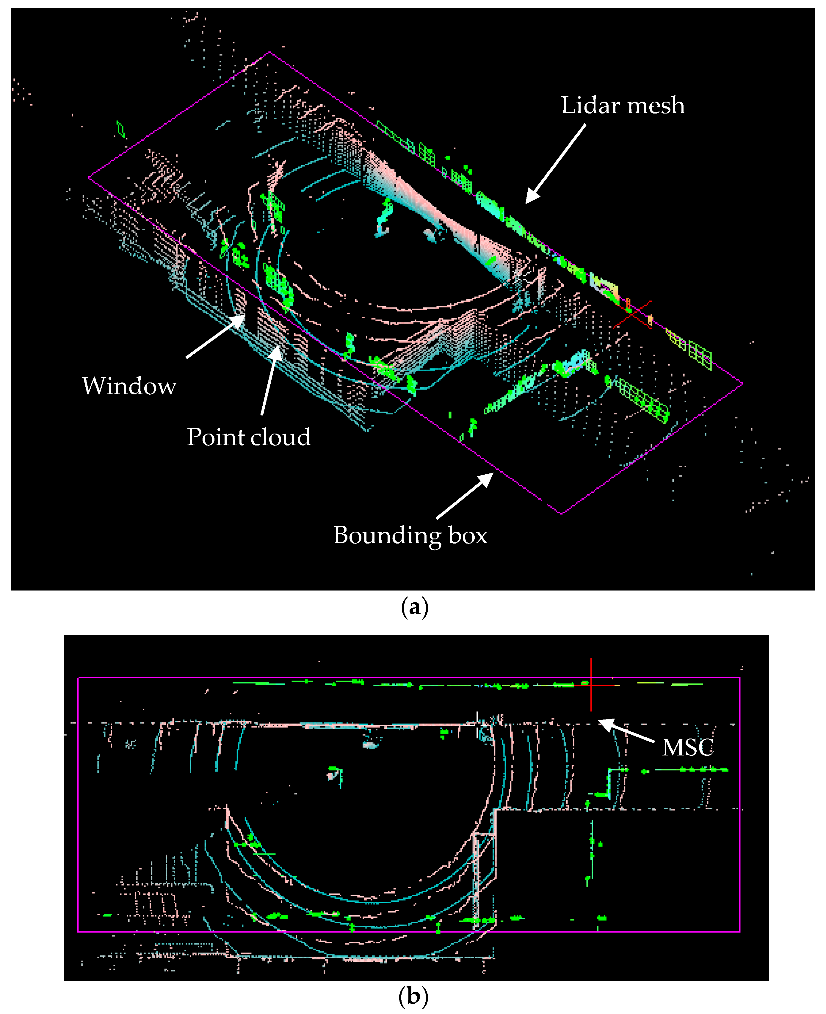
After the filtering, we can determine a bounding box for the mesh , which is formed from the envelope of the cloud points collected during the sampling time T. It is also assumed that the LiDAR is positioned rather vertical to the ground and it is in a square room when . The bounding box is then projected on the plane. The LiDAR image projection is rotated on the plane with an angle about the axis to find the minimum area of under the rotation of . At the minimum area rotation, we determine the principal axis as the X and Y axes of this room and, if necessary, the global coordinate system as shown in Figure 4d.
After the above procedures, the normal vector of the quad is used to calibrate the pitch angle of the LiDAR which can be shaken by the vehicle vibration. We first identify the individual quads which fulfills the following conditions and categorize them into X walls and Y walls.
is a small value, which is recommended to be 0.02. Taking the average of the X wall normal vectors to obtain a unit vector and Y wall normal vectors to obtain a unit vector and taking cross product on the two average normal vectors, we are able to determine the floor normal vector as follows.
The rotational transformation of the LiDAR point from the LiDAR Coordinate System to the global coordinate system can be achieved by the following operators.
denotes the rotational transformation as follows.
The angles and with respect to the X and Y walls respectively are given in the following.
After the above transformation, we can align the initial LiDAR image and identify the axes of the global coordinate system. The minimum area method as the search for the rotation angle about the axis is valid in the initial stage of the e-SLAM. The following conditions are preferred to establish the first LiDAR post frame with good accuracy.
- (1)
- Rectangular room condition: the room where the IMR starts must be a rectangular room with orthogonal walls to allow the minimum area method to find the principle axes properly;
- (2)
- No mirror condition: the room must initially be with no mirror reflecting the LiDAR ray. Without this condition, the aliasing LiDAR data can misinterpret the rectangular room.
These conditions may be unavailable in a situation where the IMR is started from the center of the lobby or an open space as shown in Figure 5a. However, in many situations, there are good long reference walls, the minimum area method will bring the bounding box to align with the longest wall as shown in Figure 5b. On the other hand, if there is a mirror in the initial position, then the aliasing LiDAR data that expand the room can mislead the minimum area method to an incorrect rotation as shown in Figure 4e. Drawbacks of the minimum area method include rotation error, the fluctuation of the rotation due to the unclear wall information, and the large angular error due to the envelope of the LiDAR image which is not rectangular in the plane projection.
2.4. Wall Corner as Land Mark
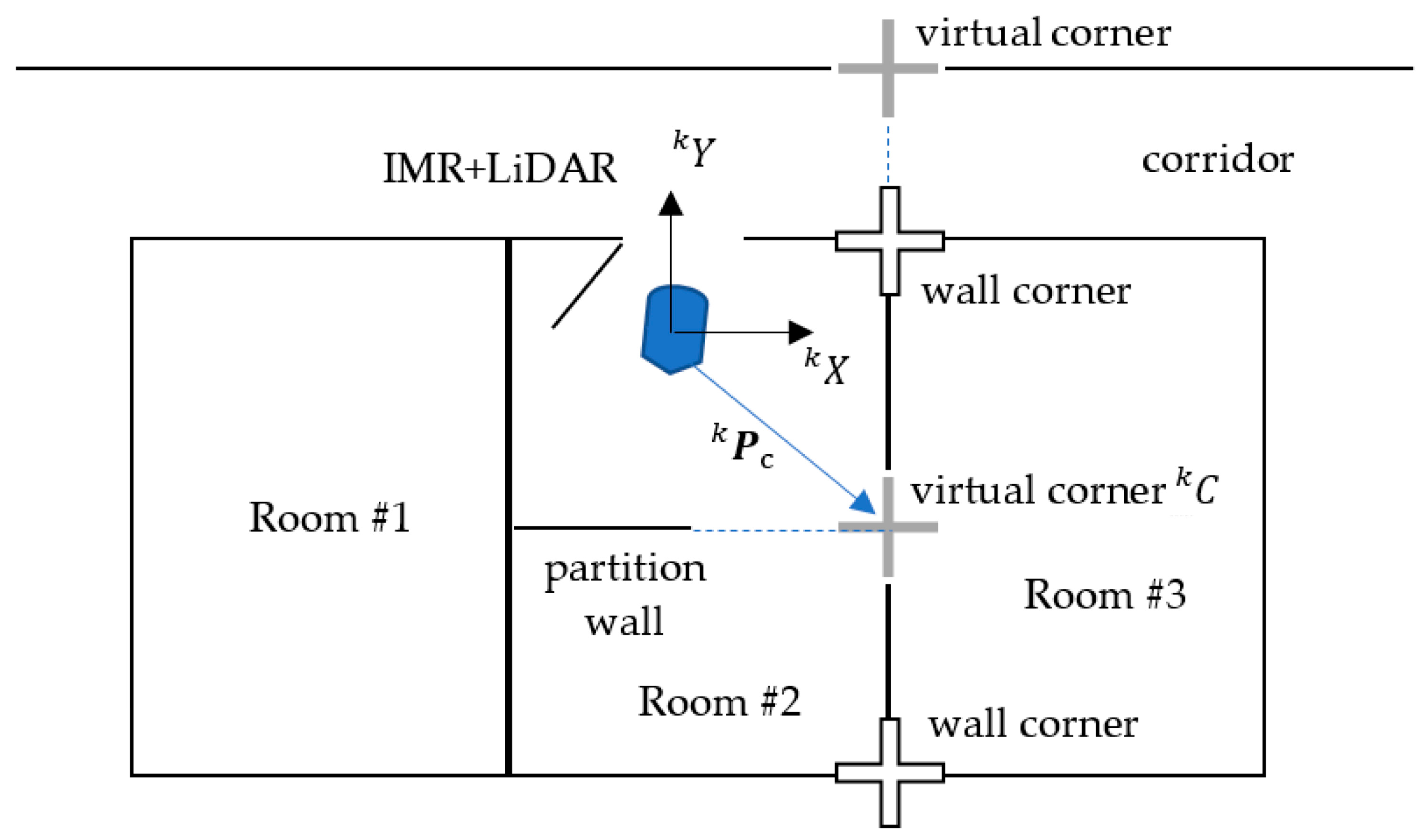
The intersection of X and Y walls are the wall corner, which can be either an existing or a virtual corner. For example, there could be a wall on the corridor referred to as the X wall as viewed from the room while the other side of the corridor walls are referred to as the Y walls. There are not any actual corners, hence, called the virtual corner in the corridor as shown in Figure 6. The wall corners or virtual corners can be utilized as the land mark of the translation calculation, that is, how far the IMR (indoor mobile robot) is moving away from or approaching a known location landmark. The walls are extracted from the quads which are marked as the X walls and Y walls.
The importance of the wall is given with a weight proportional to the ray distance which cannot be affected by the rotation pivoted at the LiDAR location. Hence, the histogram on X and Y directions may be written as follows.
The histograms have their stationary values defined as follows.
These stationary values can be sorted to obtain a set of wall corners or virtual corners as follows.
The displacement and satisfy the following conditions in pose frame.
In the set of corners, is defined as the location of the most significant corner (MSC) discovered at k-th sampling time. satisfies the following minimax condition.
Note that is a feature corner which is only an abstraction that the feature identification shall be achieved either in the histogram correlation or the LiDAR image comparison.
2.5. LiDAR with IMR Navigation
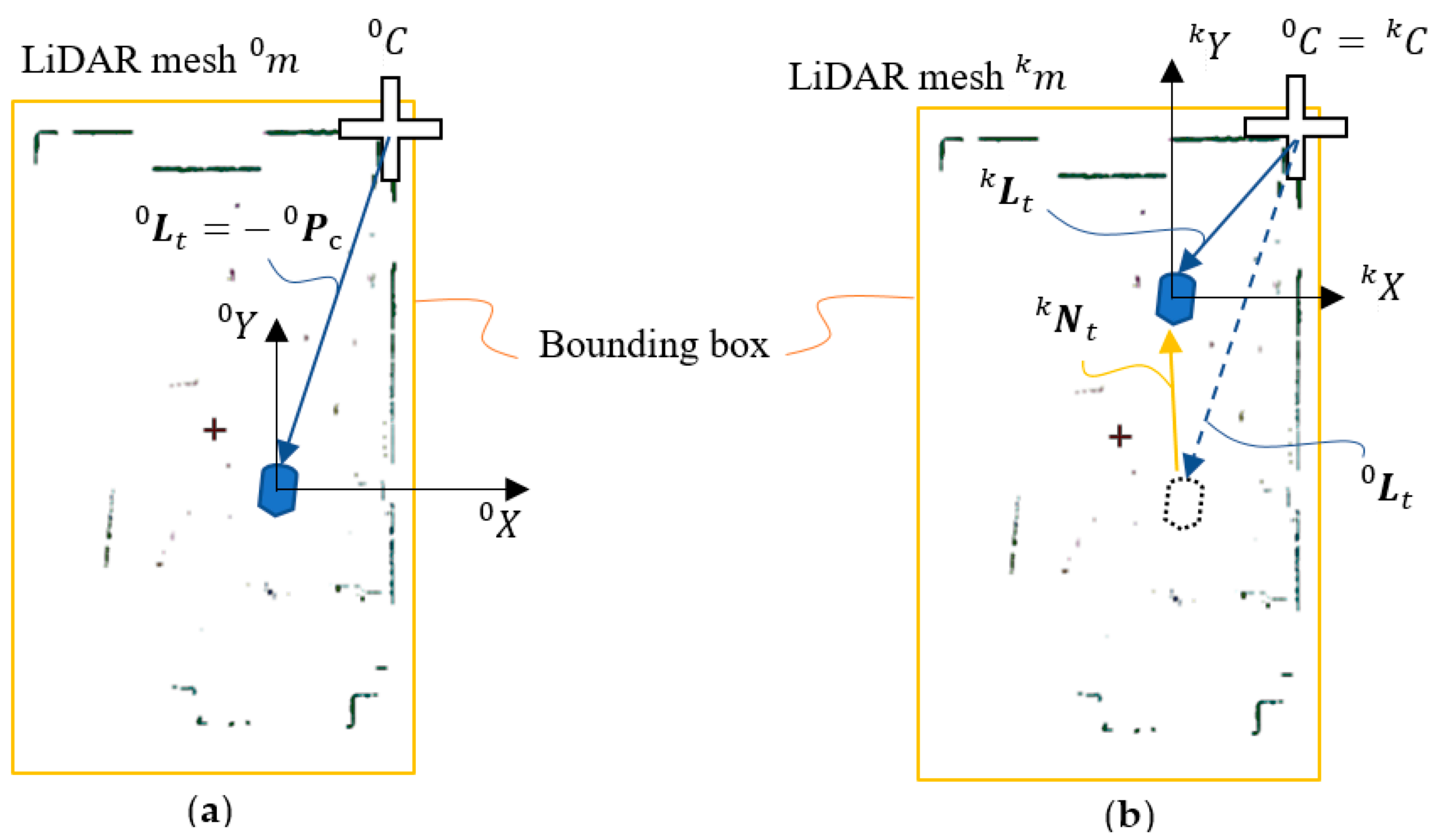
In the initial stage, i.e., , the position of the most significant corner can be used to define the pose frame when is derived from the minimum bouning box . The pitch angle is assumed eliminated during the mesh conversion process stated in Section 2.3 “Mesh Projection”, which is set to zero. Hence, the LiDAR pose frame is reduced into a three-dimensional tensor as follows.
The initial pose frame indicates that the origin of the pose frame is located at and offset with respect to the coordinate system when applying the rotation of angle about . The displacement and azimuth rotation of the LiDAR pose frame during the later IMR navigation are calculated according to the initial pose frame .
denotes the translation of LiDAR.
The initial position of the IMR or LiDAR is located at , which is the origin of the pose frame . The initial orientation of LiDAR may be derived from the zero-azimuth angle direction relative to the X axis. In case that the most significant corner remained in the k-th sampling time of the LiDAR pose frame as shown in Figure 7, the translation and the rotation angle of the IMR or LiDAR navigation can be written as follows.
It is convenient to attach the LiDAR pose frame to the actual pose of the IMR in the k-th sampling time. The translation and rotation can be calculated through the coordinate transformation such as the conventional robotics. When the LiDAR transformation and its inverse transformation are available, one is able to be move the LiDAR from one position to the other position to gather more and more points into the cloud frame. The mapping is achieved by converting the LiDAR point cloud from one scene to the other. The mapping becomes practical when the following two assumptions are fulfilled.
- (1)
- The continuity of the rotation between LiDAR pose frames;
- (2)
- The consistency of the most significant corner tracking is maintained even when the most significant corner changes through time.
To ensure both assumptions, the consistency of point cloud information has to be used in the verification. However, variations of the environment, such as objects moving, human coming into or leaving the scene, can create uncertainties to the consistency comparison. We then need a stochastic process to help us estimate the pose from the previous time to the consecutive time. Following the stochastic estimation, the rotation and translation finding procedures are discussed in the following sections.
2.6. Linear Quadratic Estimation for IMR Pose Prediction
The Linear Quadratic Estimation (LQE) may be applied to predict the LiDAR pose and its derivative through the following update scheme.
is the actual pose computed through the rotation and translation computation, which will be introduced in later sections. The actual velocity may be updated using backward difference method and can be set to zero when it is not observed by the observation matrix .
is the Kalman gain at the k-th sampling, which is updated as follows.
is the prior error covariance matrix at the k-th sampling, which is given as follows.
is the posterior error covariance matrix at the k-th sampling, which is updated from the prior error covariance matrix as follows.
The transition matrix can be derived from Newton’s law of motion as follows.
The observation matrix may observe only the pose and not the velocity of IMR as follows.
The noise covariance matrices and are related to the variance of the position and velocity individually. LQE yields the prediction of the position as well as the rotation of the IMR which carries the LiDAR. The most important feature is that LQE can yield a filtered result of prediction which leads to a range for the rotation and translation search of the LiDAR mesh .
2.7. Rotation Update Scheme Based on LQE
As stated previously, the minimum bounding box area method can be used in finding the rotation only during the initial stage. For the remaining steps , we need to find the rotation based on the previous rotation angle which is the previous LiDAR orientation. can only be in the range of in the vicinity of , where is a factor of allowable variation and is the allowable rotation change when the previous rotation speed is zero. We can apply a rotation angle to rotate the mesh points as follows.
is the estimated rotation from the Kalman filter denoted as in Figure 8. The purpose of the rotation test is to find the minimum rotation difference between and allowing the histogram values of the walls, i.e., and , to be maximized. These can be done from one of the three methods stated as follows.
- (1)
- Minimum bounding box area method: the same method for the rotation finding as in the initial stage, which may be working for the early time when is small;
- (2)
- Maximum total histogram value: maximize ;
- (3)
- Maximum total number of quads on the bounding box; maximize the members in the set .
The practical way is to use all three methods simultaneously and verify which one satisfies Equation (29). If all three methods fail, then find the which minimize . The incremental rotation can bring the mesh to align with the previous LiDAR mesh . The remaining difference between and is the coincidence of the wall corners between the meshes.
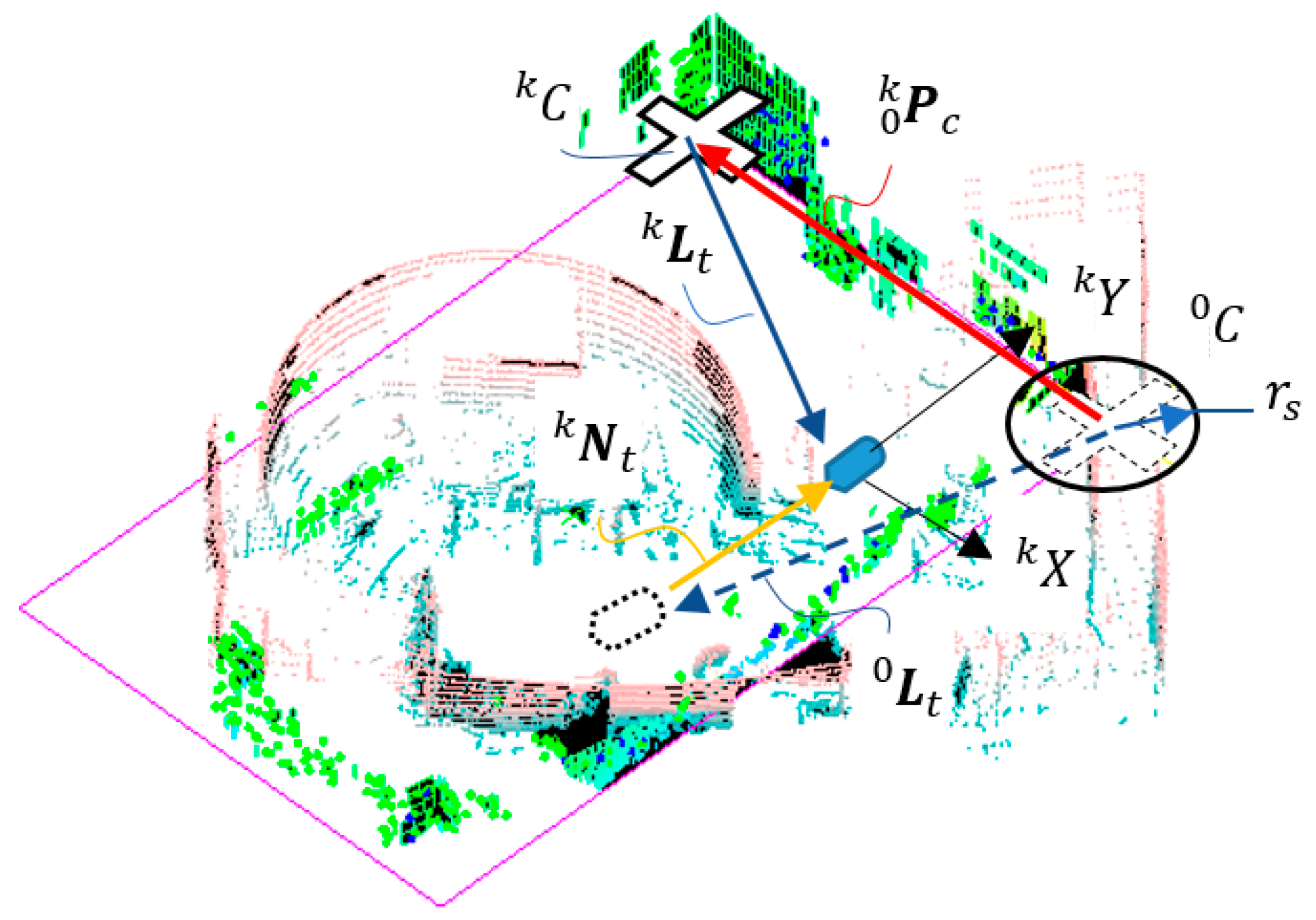
2.8. Translation Update Scheme Based on Most Significant Corner (MSC) Transfer
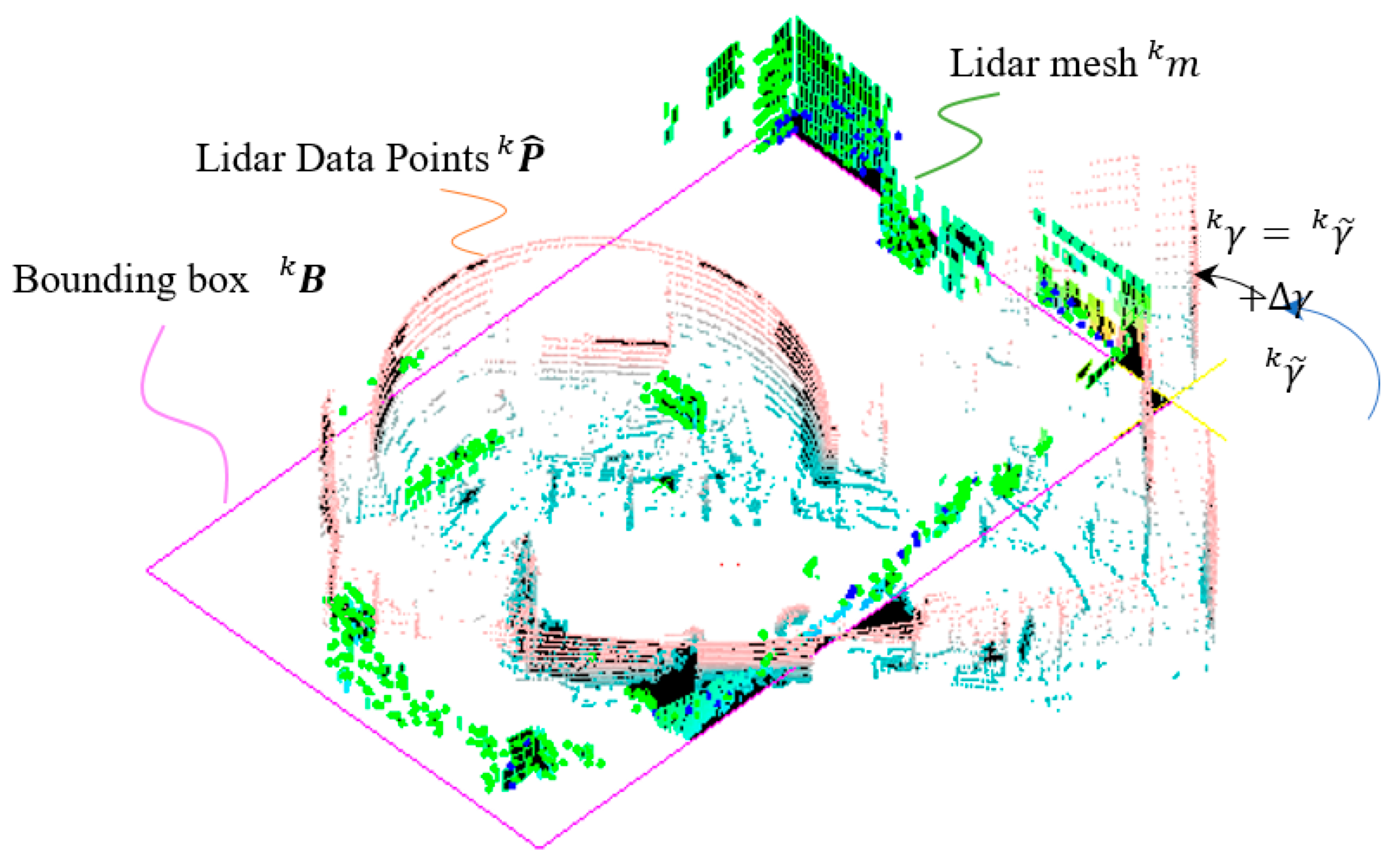
In case that the is not any more the most significant corner in the k-th sampling as shown in Figure 9, we will have to update the IMR navigation in the following way.
The vector opposite to is the location of the most significant corner in pose frame Note that is a feature corner which is only an abstraction that the identification of the feature shall be achieved either in the histogram correlation or the LiDAR image comparison. When the LiDAR image comparison of the entire space is not computationally efficient, then the histogram correlation may not be accurate enough. An efficient way to distinguish a feature corner may be done while updating. In the linear quadratic estimation, we are able to estimate the IMR navigation velocity from Equation (23). Based on the estimation, we can predict the location of the in pose frame through computing
The feature corner shall be in the neiborhood of in LiDAR pose frame . We only check the vicinity of of the histogram and to locate the wall corners , which must satisfy the following condition.
denotes the radius of tolerance of search. The one which uses histogram search is more efficient, thus can be processed before the LiDAR image comparison. It could sometimes happen that the feature corner is missing in the frame of since it may be blocked by moving objects such as humans. We then have to locate the feature corner in LiDAR pose frame as follows.
On the way that IMR navigates, the MSC can change from one to the other and sometimes it can even loop back to an early used MSC. The update scheme for translation can then be written as follows.
is a zero vector when the MSC is not changed from pose frame to .
The LiDAR images are comparing to the LiDAR mesh and projection on their individual XY plane and finds the maximum correlation between the mesh image, which is the same as what has been done in conventional image processing. The translation found between and can be thought as . The image of LiDAR mesh can be first projected to the XY plane and compared to one another after the rotation update. The image correlation between two projected pixel images can yield the translation between and in a precise way, however, this is a time-consuming process and is only acquired when necessary.
3. Floor Management
There could be only one LiDAR pose frame for the entire floor to which all LiDAR mesh data will be mapped back. However, the maximum number of quads is a finite number according to the azimuth and number of rings. In case of a complicated space such as the office building, due to several rooms and partitions, it becomes impossible to map all walls of different rooms into one simply connected mesh. Multiple connected meshes are necessary to contain the complete information of different rooms. As for floor management, we would need different room mapping even if there is only one LiDAR pose frame , called the base pose frame.
As stated in Section 2.2, three proposed conditions are applied as the filters to form the LiDAR mesh, which include (a) the cluster condition that is used to remove the unwanted information from the mirror reflection and those from the walls outside of the transparent windows, (b) the vertical condition to remove the passer-by and the static furniture data, such as sofa and tables, and (c) the aspect ratio condition to remove the stairstep surfaces which are not continuous walls. The adjustment of parameters used in the three filtering conditions can improve the adaptation to office buildings of different kinds. The preferences stated in Section 2.3 are that the initial location we find to turn on the IMR is better to include the rectangular room condition and the no mirror condition for increasing the estimation accuracy of the minimum area method. Since the base pose frame is the basis of the IMR exploration, it determines the accuracy of the Lidar mesh map for a room. IMR navigates in the environment with assumed conditions that (1) the rotation between LiDAR pose frames is continuous, i.e., it will not fumble, and (2) there is at least one most significant corner that we can use to form the LiDAR pose frame and track the IMR navigation. These assumptions and presumptions about the environment are not limiting the use of e-SLAM, while on the other hand, they are the dimensions to improve the applicability of the e-SLAM.
3.1. Single Room Mapping
After a series of point cloud conversions of multiple points of different ’s and same are mapped into base pose frame . is the LiDAR data point obtained in pose frame and converted into the LiDAR data point in pose frame . is a homogenous transformation from pose frame to the pose frame , which can be written as follows.
The total LiDAR image could be computed from the average of all range data on the same and as follows.
denotes the number of non-zero range data from all pose frame . In order to filter away the LiDAR data which are from the moving objects such as passer-by, we extract the LiDAR mesh data representing only the walls via the filtering conditions including the vertical condition and the aspect ratio condition as stated in Section 2.2. The wall mesh of the same area is repeatedly obtained from different LiDAR pose frames as the IMR navigates, and thus, the wall smoothing is achieved when the moving objects are far away.
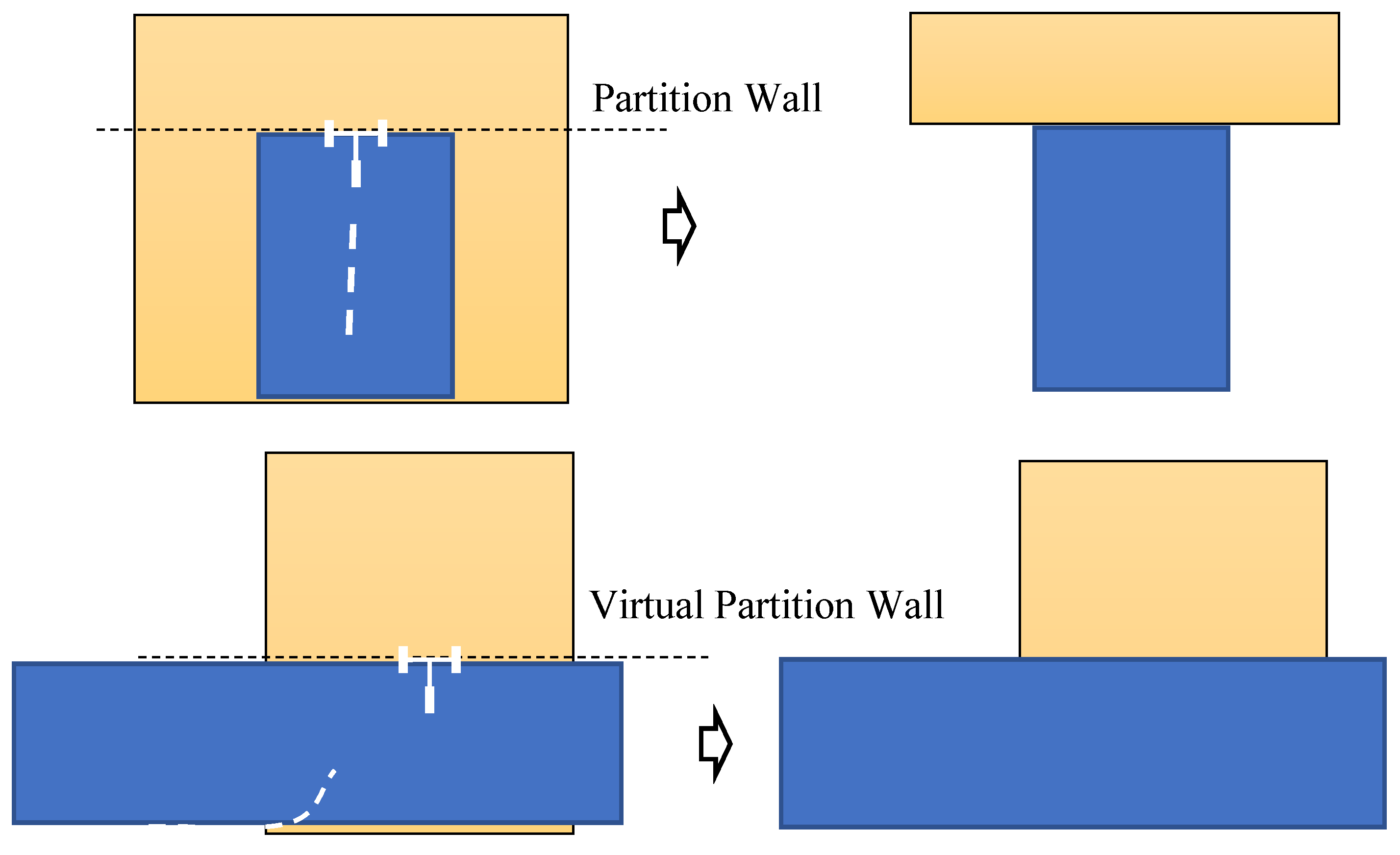
3.2. Room/Corridor Segmentation
The range data of a single ray will be used to represent two walls, as stated in the previous section. There is a need to separate rooms that are partitioned by walls. We also need to label each room with an individual room index providing that the room adjacency matrix is documented. It may be convenient to setup the IMR travel distance for determining the bounding box , and after determining the bounding box, the room size is fixed. It is then using the information of the IMR crossing the boundary of the box to determine the wall partitioning the rooms is shown in Figure 10. When the corridors are partitioned into two rooms, there is no actual wall, however, a virtual wall is partitioning the space. As shown in Figure 10, when the IMR is leaving an initial room (blue box) and going forward for further exploration, the data on the left and right sides of the room are the LiDAR noise came from either the mirror reflection or the transparent windows. The partition wall that provides a border to the new room can filter away those noise and initialize the LiDAR mesh for a new room reached, i.e., a corridor (yellow box) in this case. As shown in Figure 10, when the IMR is turning left to a new room (yellow box) as an example, the previous data obtained from the LiDAR visible region shall be granted to the early room (blue box). A virtual partition wall (not existing) yields an open space in the mesh data storage for the new room to form its new room boundary.
4. Experiment and Comparison
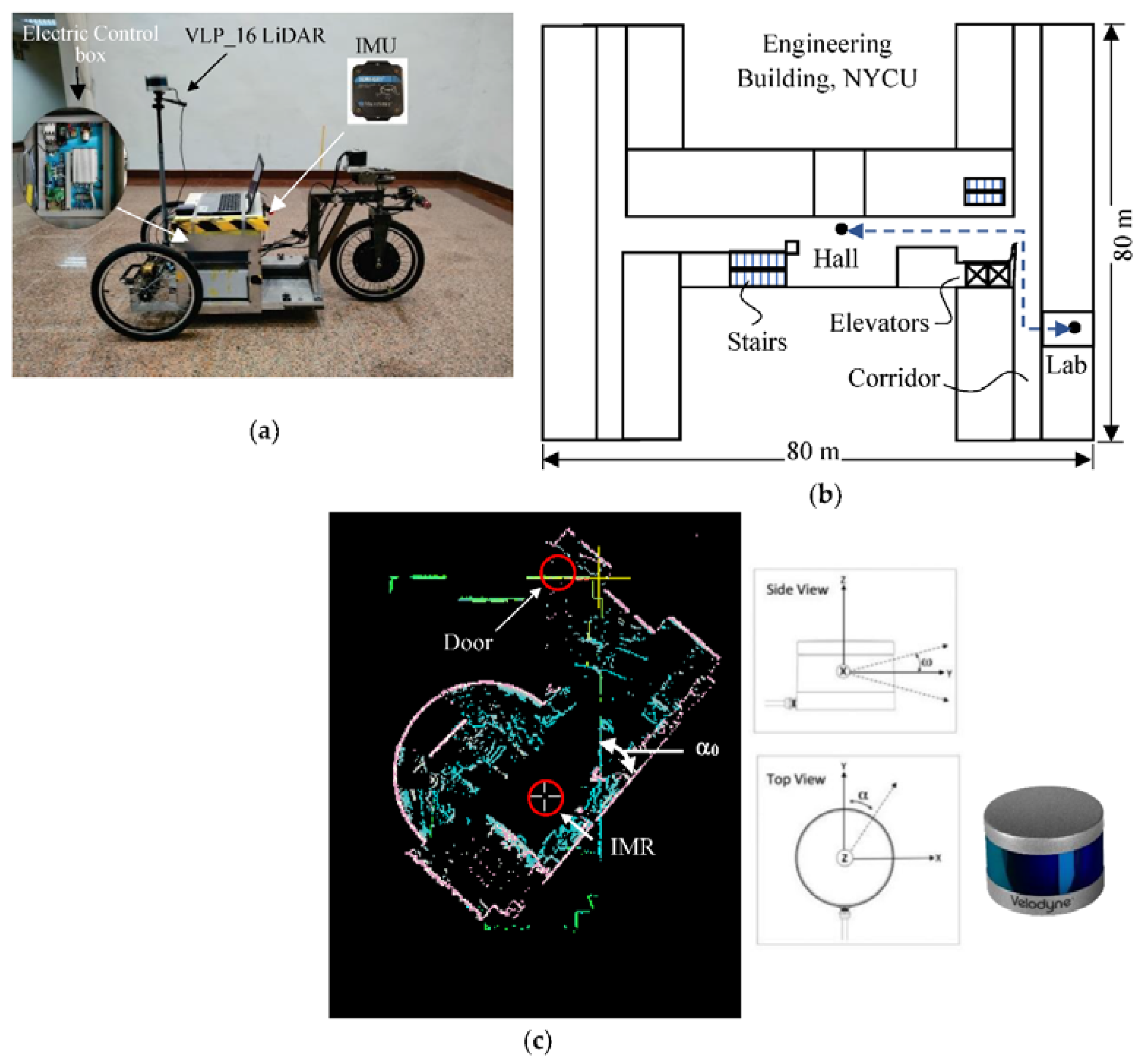
A tadpole model of a tripod IMR is used in the experimental study. A traction in-wheel motor is applied on a single rear wheel which is integrated with an electric steering system on the top of the steering column, and two passive wheels are installed on the front wheel with 20 × 1.65 tube tire type. A VLP_16 LiDAR with 16 rings made by Velodyne Inc. is positioned onto the center of the front axle with a total height of 1.65 m from the ground as shown in Figure 11a. The tripod IMR has a turning radius of 1.2 m and is driven by people during the tests. There was an electrical control box that enclosed a 24-V drive with EtherCAT communication protocol for steering, a 48-V drive for traction controls, a 45-Ah 48-V Li-ion battery for traction system, and an IMU (Microstrain® 3DM-GX1) [71]. The IMU integrating three angular rate gyros with three orthogonal DC accelerometers, which were used for the later verification purpose but not for the localization purpose. The test environment is the Engineering Building V in the Kwang-Fu Campus of the National Yang-Ming Chiao-Tung University. It is an I-shape building with two wings and a connection section. The experiment was performed on the fifth floor with a floor area of around 5000 where the top view is shown in Figure 11b. The wall material is made from concrete and white fiber cement layered onto the wall surface with a solar reflectance of 0.40. There are four tests moving repeatedly from the hall to the lab. A simple text file in pts format is used to store point data from LiDAR scanners. The first line gives the number of points to follow. Each subsequent line has 7 values, the first three are the (x, y, z) coordinates of the point, the fourth is an “intensity” value, and the last three are the (r, g, b) color estimates. The intensity value is an estimate of the fraction of incident radiation reflected by the surface at that point where 0 indicates no return while 255 is a strong return. In the lab, there is a dome screen made of wood, which occupied one quarter of the lab space. There is also a mirror on the wall adjacent to the door which can produce fake feature data by reflecting the laser light. As shown in Figure 11c, the IMR is in its upfront position in the room toward the door. The angular difference between the LiDAR data and the LiDAR mesh is the initial azimuth angle . After the initial azimuth angle is obtained from the proposed method in Equation (15), one can reinstall the LiDAR by manually rotating the LiDAR fixture on the IMR to align the zero-azimuth angle to the upfront direction. There will still be some inaccuracy left behind needed to be verified through the experiment.
There are two tours from the lab to the hall and from the hall to the lab. Each of the tours has been performed twice. The intent of the course of the experiment is to prove the generality of the proposed method as follows.
- (1)
- In the course of the experiment, IMR went from a door-closed room to the corridor after the door is opened. The challenges include the complication of LiDAR mesh formation from the closed area to an open area, and also the floor management.
- (2)
- The IMR navigates from a room to the corridor and to the elevator space where many passengers (moving objects) are presented, and then, to the lobby which is an open space. The corridor navigation is a challenging part, which has very weak MSC information when the walls do not intersect.
- (3)
- The IMR makes two 90 degree turns, one right and one left, between two complete stops. The displacement and orientation estimation of the proposed method can be fully tested.
During the tour from the lab to the hall, there are four most significant corners (MSC) found in the lab, more than 10 MSC’s found on the corridor and many other MSC’s found during the entire IMR navigation. There is one person driving the IMR manually by its handle bar which includes the throttle and brake to control the IMR. The person who controls the handle bar is at his lowest position as possible to avoid blocking the LiDAR rays from shooting on the high side of the walls.
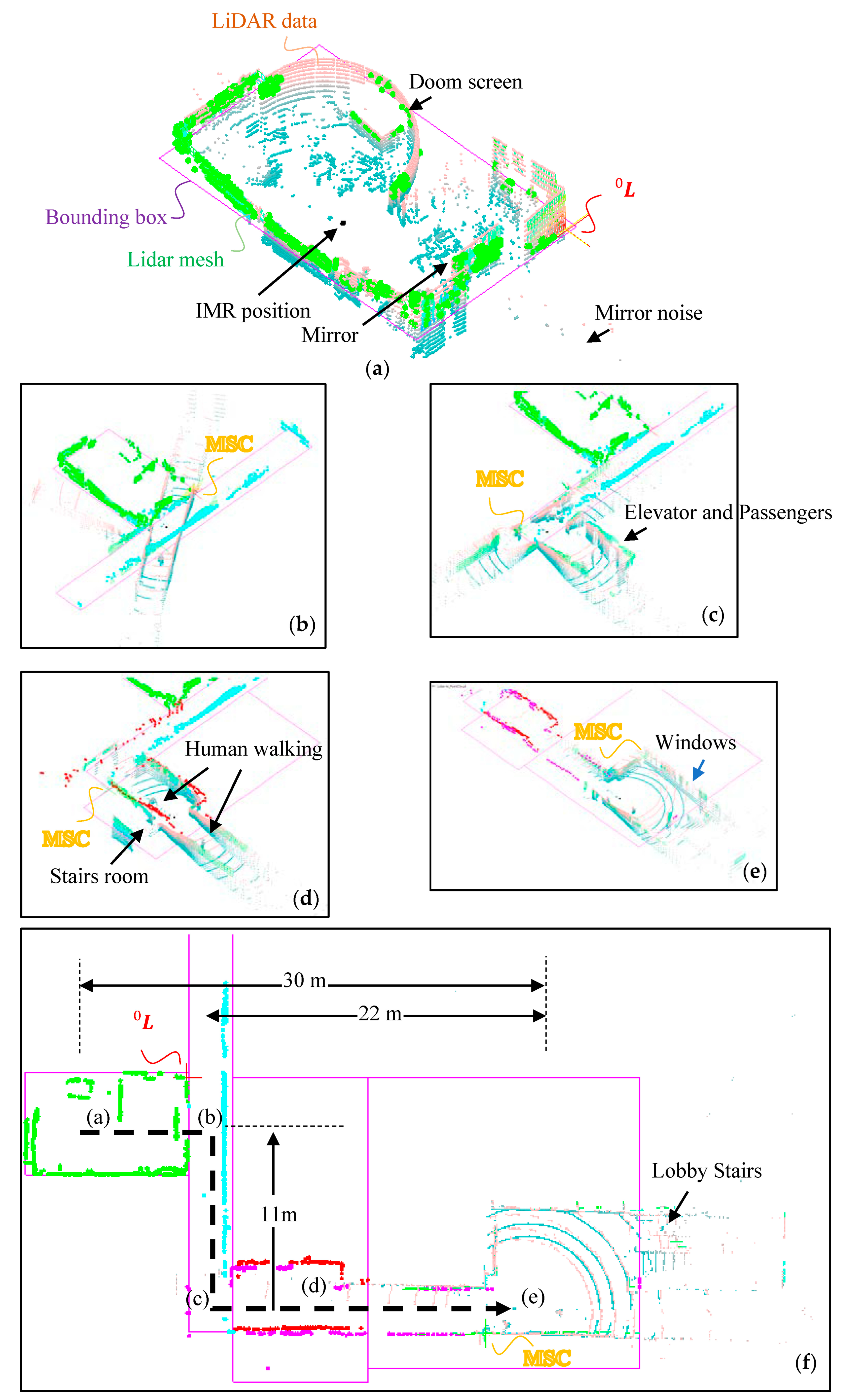
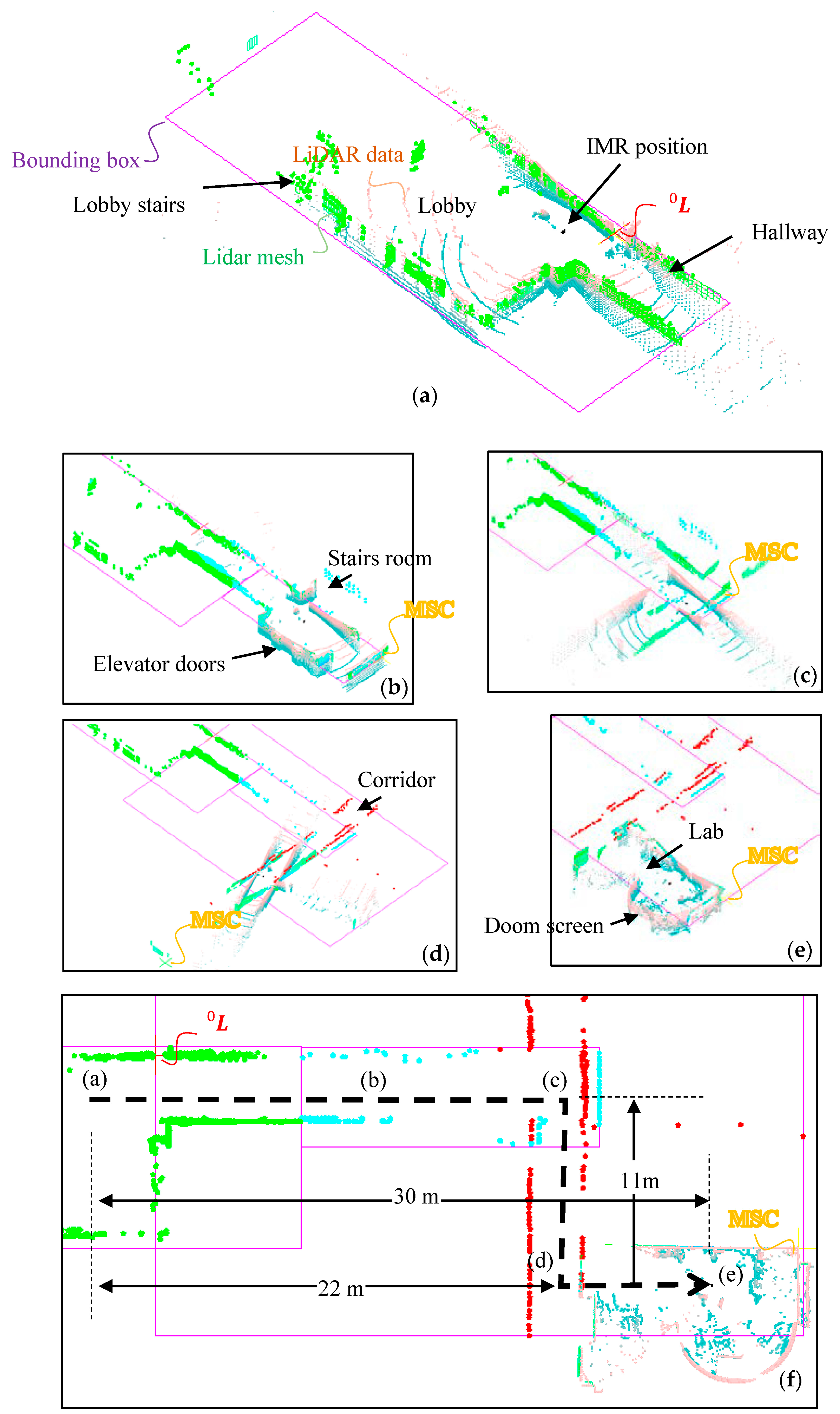
We chose only point clouds from positive ring angles to form the LiDAR mesh in the experiment. We assumed that the high portion of the wall poses more wall corner information than the lower portion does. Thus, in VLP_16, there are degrees that can be utilized to form the mesh. In different experiments, we have collected 550 to 750 LiDAR data frames from four different IMR navigations within 80 to 120 s. The frame rate is around 5 data frames per second that we recorded. The total distance accumulated during the navigation is about 45 m. The average speed of the IMR is 2 kph (km/hour) which is a medium speed in the indoor mobile robot application. During the navigation, there are two T-junctions to turn and the IMR will stop when there are people walking by. The highest speed of the navigation was 4 kph during the course. In Figure 12, we demonstrate the tour from the lab to the hall. There is a dome screen which is nearly one quarter area of the lab, which also provides a counterexample of vertical walls in this room. There is also a mirror on the side of the entrance door, thus providing a LiDAR error source. The base pose frame is chosen to be the first found MSC when IMR starts the navigation, which can also program to other locations in order to have a better resolution of the entire space with a different room. In Figure 12a, we can find two images, for which the real time LiDAR data and LiDAR mesh were calculated. They almost coincide with each other just because when the IMR started navigation, the LiDAR azimuth angle is pre-aligned to front. The alignment of LiDAR azimuth angle to the front of the IMR is not always true in applications of multiple LiDAR systems. Indeed, it is very difficult to align the LiDAR azimuth angle precisely to front and the misalignment can be calculated during the first minimum bounding box test. The angle between the bounding box and the IMR is the misalignment angle. In Figure 12b, we demonstrate the circular motion of the IMR. During the circular motion, the IMR merely moved and the LiDAR scanner senses only the rotation. In Figure 12c, when the IMR reaches the T-junction between the hall way and the corridor, the IMR rotates again. Between Figure 12b to Figure 12c, there are many number of MSC jumps since the corridor does not have the significant MSC which is seen by the LiDAR scanner. Thus, MSC may jump to the frame of the door and also to the bulletin box on the walls which indeed needs the LiDAR mesh image comparison between the room and the current rotated LiDAR mesh data stated early in the final paragraph in Section 2.8 “Translation Update Scheme based on Most Significant Corners (MSC) Transfer”. In our software, we will send a beep sound out from the controller of the IMR which signals the difficult situation and possibly error translation updated. In practice, there will be many other sensors such as GPD and IMU in addition to the LiDAR scanner helping advise on the correction translation. However, in this experiment, we purposefully do not acquire the information from the other sensors to fully understand the reliability of the e-SLAM method for the localization of IMR. In Figure 12d, when the IMR is moving to the elevator room, there are passengers waiting for the elevator, while one of the passengers was entering the elevator, thus, the elevator door was opening and closing. In Figure 12e, IMR reached the hall and before that there was a person walking through the hallway and encountered the IMR. It can be seen that the floor management is performed to separate the entire course into 4 rooms where one is adjacent to the other. At the top view of the map produced from the e-SLAM as shown in Figure 12f, there are several things found which shall be discussed.
- (1)
- The LiDAR azimuth angle is not zero. From the top view of the LiDAR mesh image, it is found that the final LiDAR data are not perfectly aligned with the map.
- (2)
- The room near to the base pose frame gets better resolution. It can be observed from Figure 12f that the Lab with more green dots representing the LiDAR quads and the lobby received fewer dots. It is because the resolution of the LiDAR quad is limited by the distance from its base pose frame . We can have a quad with one meter height because the distance was 30 m away from the base pose frame and the ring angle resolution is 2 degrees.
- (3)
- There is noise involved into the room bounding box which can be caused by the reflecting image from the shining surface such as windows of the bulletin.
- (4)
- The maps of room (d) and room (e) with different colors overlapped each other. It is also observed from all adjacent rooms. The overlap region can allow us to tell the dislocation of the translation update scheme.
- (5)
- The room segmentation is determined by the IMR travel distance and the bounding box is applicable when the rectangular room is detected. However, it failed to box precisely the space when it was on the corridor and the hallway. This can cause an even bigger problem when IMR travels on a long corridor.
The other test is conducted by moving the IMR back to the lab. In Figure 13a, we see that the LiDAR data on the vicinity of the hallway had ring arcs in different wave spacings. The denser ring arcs are the ceiling. The sparser ring arcs are the hallway. It looked like the hallway had an inclined floor surface, which is actually flat and horizontal to the ceiling, since the wave spacing changes of both floor and the ceiling are the same. In Figure 13a, the rectangular bounding box can still be found in even a very complicated space. The base pose frame is also chosen to be the first found MSC when IMR starts the navigation. However, this time, the MSC formed is a virtual corner which is the intersection of non-touching walls. In Figure 13b, the IMR travels through the hallway and sees the stair room, which is then moving to the T-junction between the hallway and the corridor as shown in Figure 13c. In Figure 13d, the IMR reaches the door of the Lab and IMR continues to go further into the Lab. Figure 13f shows the top view of the map produced from the e-SLAM, it can be observed that the room index is not successfully provided to the Lab because of the low resolution of the Lab when it is far away from the base pose frame . It is also observed that the third room including the hallway, the corridor and the Lab cannot be separated from the hallway because there is no good separation line found when the IMR moved from hallway to the corridor. The T-junction occupied by the hallway room blocked the corridor to be formed as a unit of room.
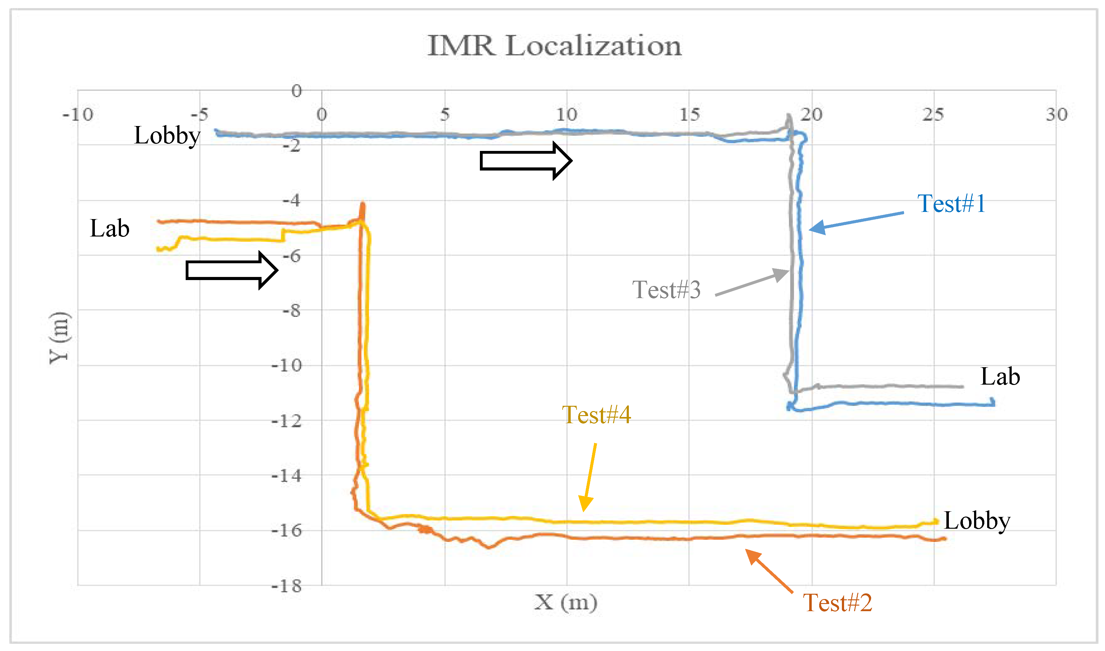
The other two tests are repeated from the previous two tests, which are used to compare the rotation and translation reading of the IMR based on the active localization based on the e-SLAM method. Each of the tests are performed with different navigation speeds and waiting times when encountering moving persons, with different number of data frames from 550 in Test#3 to 750 in Test#1. The results are compared in Figure 14, the x- distance between the lobby anchor points to the Lab anchor point is about 30 m, the lobby anchor point to the T-junction is about 22 m, and the T-junction to the position in front of the door is about 11 m. Each time, the IMR trajectory may be different by 1 m. The direction of IMR was rotated at 180 degrees every time before the next test started. Thus, their coordinate systems are different in x-direction, i.e., the x-direction of the tests from lobby to Lab is opposite to that of the tests from Lab to lobby. They matched in dimensions of the space within meter accuracy. The amount of error may due to the causes in the control and analysis.
- (1)
- The trajectory difference: There have been real situations in different IMR navigation tests including passer-by, elevator passengers, and environmental conditions such as door open/close. These situations caused the non-holonomic robot control system to detour from the predefined runway, which has been recorded in video files allowing replay to verify. So far, it contributes 50% of the error based on the video replay data.
- (2)
- The starting and ending position difference: The starting positions are marked before each test, however, precisely arriving at the same mark as the ending position is difficult for the IMR due to the position control being done manually using electrical throttle and brakes as stated before. The differences contribute 30% of the error so far.
- (3)
- The e-SLAM localization error: There still were some errors found from the simulation analysis in the localization process. These errors will show the LiDAR meshes slightly shaking on the screen in the simulation streaming. The computation will contribute 20% of the error based on observing the simulation streaming.
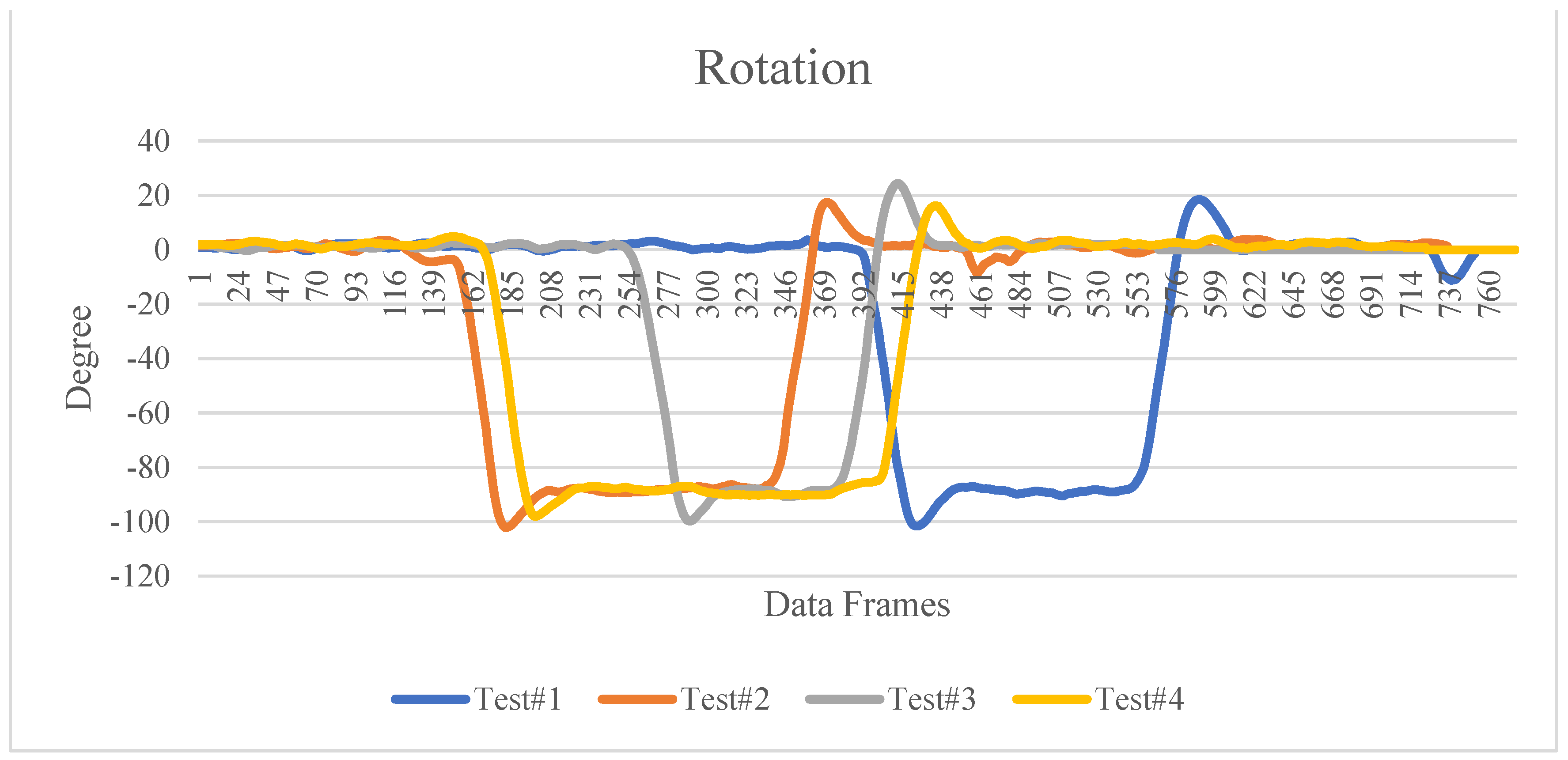
The error of Test#4 is largest among all four tests, which may be caused by the e-SLAM localization error. Thus, we may conclude that the deviation of the active localization of e-SLAM is within 50 cm. This error may need the compensation from other sensors such as IMU or high precision GPS to compensate. It may also acquire the precise calibration of the locations from the image recognition of fiducial marks. As for the rotation based on the active localization, all four tests are done by first going along a straight line with no rotation, then turn to the right by 90 degrees, then travel on the corridor in a straight line, turn to the left by 90 degrees, and then going straight. Since they have different number of data frames, they cannot be compared at the same time count. The result in Figure 15 shows that there is always an overshoot during rotation which was actually happening during the IMR navigation. The maximum rotation overshoot is around 20 degrees. Comparing to the actual data frames played as a movie, we can observe only less than 5 degrees of error for the rotational localization, thus, we can conclude the error of rotation is within 5 degrees. The error may be compensated by the gyroscope in the high precision IMU. The initial azimuth angle does not affect the relative rotation information between LiDAR pose frames which yields the rotation of the IMR. Under the condition mentioned previously that the LiDAR azimuth angle is non-zero, the rotation results as shown in Figure 14 have two steady states on precisely 0 and 90 degrees which are not affected by the LiDAR azimuth angle . Hence, further calibration of the initial LiDAR azimuth angle is unnecessary, and it can reduce the maintenance work.
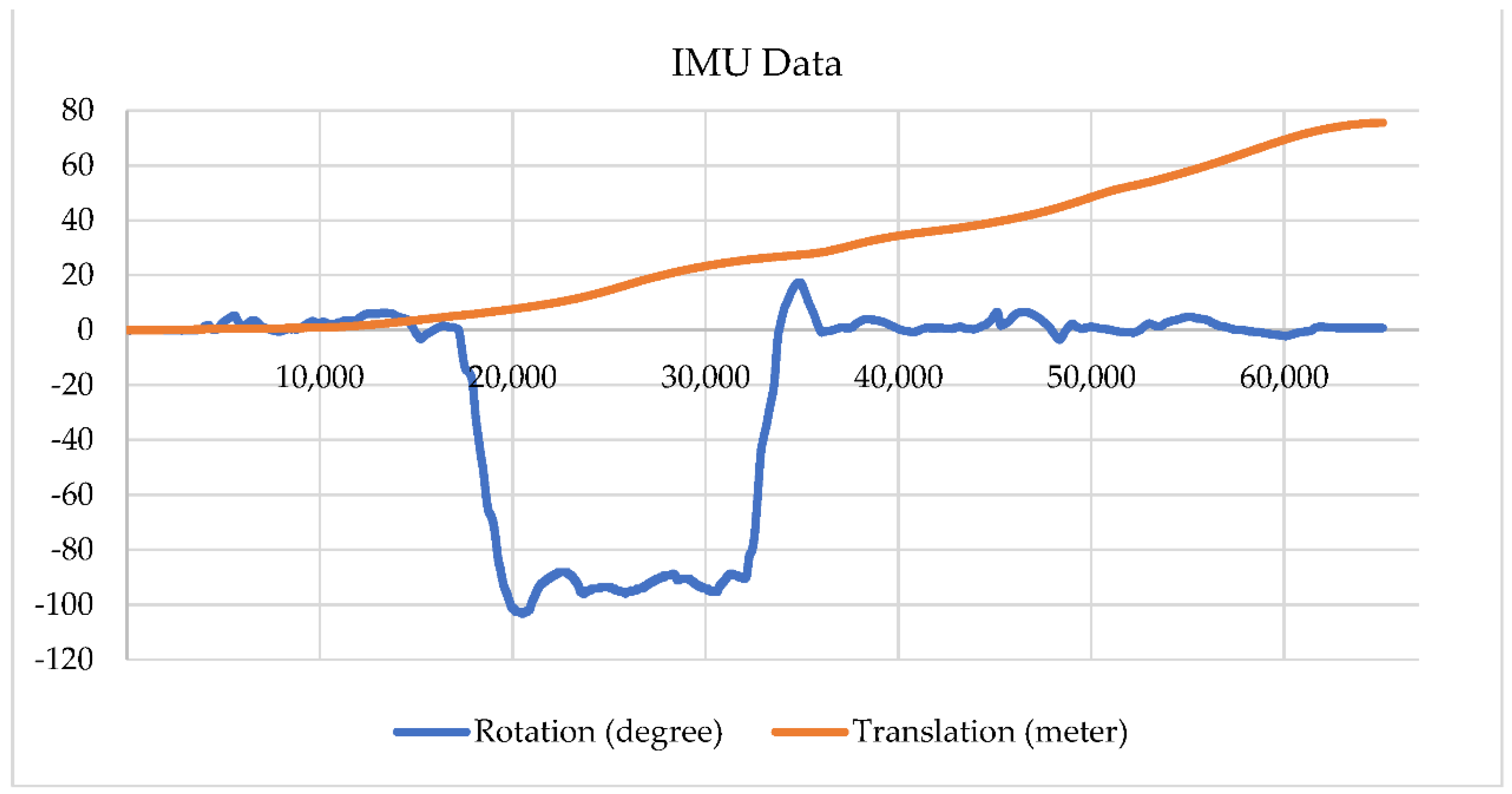
In order to show the significance of the proposed system, we also show the comparative data obtained from the IMU shown in Figure 16. The rate for Euler angles is 100 Hz and for accelerometer data is 350 Hz from the IMU. The horizontal axis is the data count instead of the actual time. Figure 15 and Figure 16 are from different sampling rates collected from different routines, thus, they had different data counts. The IMU data were recorded on the tour of Test#4. It is found that the rotation angle (blue line) in Figure 16 is coarsely comparable to the Test#4 result (yellow line) shown in Figure 15, however, IMU rotation data are noisier than those found from the e-SLAM result on straight line sections. The overall travel distance on the tour of Test#4 shall be 41 to 42 m according to Figure 12, which is different from the translation of 75 m calculated from the accelerometer result shown in Figure 16. The IMU travel distance error may be due to the calibration of the accelerometer. As a result, the e-SLAM method proposed in this paper is suitable for position accuracy as well as rotation stability. The e-SLAM is not an integral-based sensor, which is free from accumulation error.
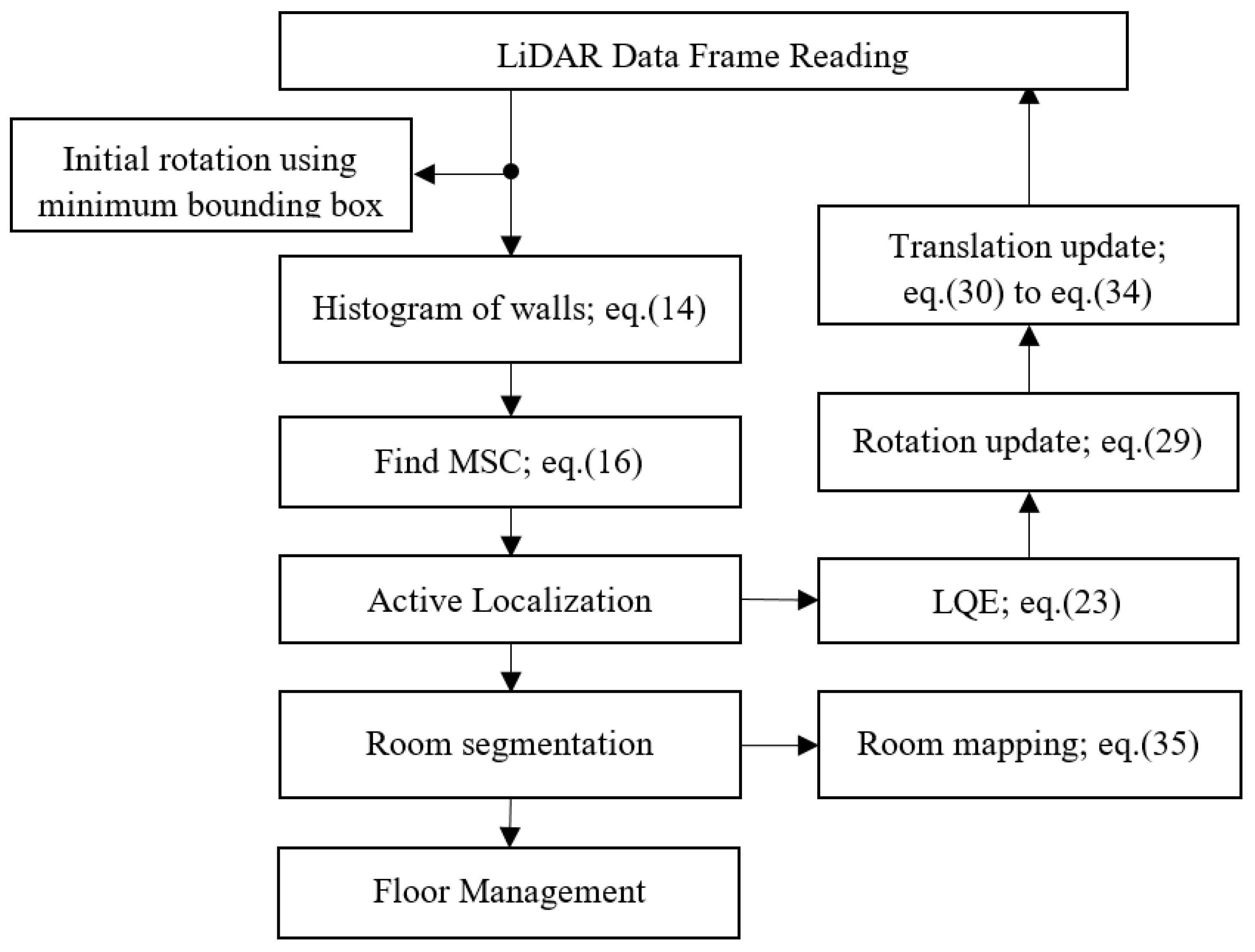
In summary, the e-SLAM includes the procedures of (1) finding the initial rotation using the minimum bounding box method, (2) finding the most significant corner from the walls vertical to the floor based on the histogram analysis, (3) choosing the base LiDAR pose frame and doing the inverse transformation to map all LiDAR data back to the room map, (4) performing the active localization based on the rotation and translation update scheme, (5) utilizing the least quadratic estimation (LQE) method to perform the localization estimation, (6) utilizing the LiDAR data XY projection image to assist the translation update, (7) performing the room segmentation, and (8) performing the floor management. The flow chart of the e-SLAM processing is shown in Figure 17.
5. Conclusions
The method of exploration-based SLAM (e-SLAM) for the indoor mobile robot using LiDAR is introduced in this paper. The e-SLAM method with the mapping using LiDAR mesh of vertical walls can trim the static furniture and the moving object from the same space of the IMR through the proposed conditions in Section 2.2 for the LiDAR mesh formation. With the help from LQE estimation on the translation and rotation, LiDAR can be the only sensor used for the active localization. The computation time is 90 s to process the longest PTS file with 750 LiDAR data frames, which recorded 120 s of the IMR navigation, using a computer with a Windows10 operating system and an Intel(R) Core (TM) i5-8500 CPU @ 3.00 GHz 3.00 GHz CPU and 4 GB memory. The software was running in a single thread executable code. The e-SLAM can achieve the real-time processing. The precision of e-SLAM is 50 cm in translation and 5 degrees in rotation. When the most significant corner in starting position of the IMR is made as the base pose frame, the maximum distance for the 16-ring LiDAR can go as far as 35 m away to persist good active localization. When the space requires more than 35 m, multiple base pose frames can be used to increase the resolution during the XY projection image comparison. The experiment was conducted during the office hour of NYCU engineering building when many moving objects such as humans and elevator doors were into the LiDAR scanning. The reliability of the e-SLAM method is preliminarily proven. There are still problems left unsolved to the future, which include the method to handle multiple base pose frame and a better room segmentation method to handle the long corridors. Nevertheless, there is a need to improve the translation update accuracy.
Author Contributions
Conceptualization, W.-H.C. and L.-C.T.; methodology, H.I. and L.-C.T.; software, R.R. and L.-J.S.; validation, H.I. and L.-J.S.; formal analysis, L.-J.S.; investigation, H.I.; resources, H.I. data curation, H.I.; writing—original draft preparation, L.-J.S. and R.R.; writing—review and editing, R.R.; visualization, H.I.; supervision, W.-H.C.; project administration, L.-C.T.; funding acquisition, W.-H.C. All authors have read and agreed to the published version of the manuscript.
Funding
This research was funded by Ministry of Science and Technology, R.O.C., grant number MOST 110-2622-8-009-018-SB. In part, this work was financially supported by the “Center for the Semiconductor Technology Research” from The Featured Areas Research Center Program within the framework of the Higher Education Sprout Project by the Ministry of Education (MOE) in Taiwan, and also supported in part by the Ministry of Science and Technology, Taiwan, under Grant MOST 110-2634-F-009-027.
Data Availability Statement
Data sharing is not applicable.
Acknowledgments
We thank IMLab NYCU graduate student Yi Chen for her help on the Lidar setting.
Conflicts of Interest
The authors declare no conflict of interest.
Nomenclature
| Symbol | Abbreviation |
| Angle formed between rings from the LiDAR center | |
| Azimuth angle | |
| LiDAR data point at n-th ring by a-th ray | |
| LiDAR transformation matrix | |
| LiDAR data point in the rectangular coordinate system | |
| LiDAR point at pose frame k | |
| Quad in mesh formed at n-th ring by a-th ray | |
| Normal vector at quad | |
| Mesh at pose frame k | |
| Boundary box at mesh | |
| Angle for rotation at XY plane for LiDAR image projection | |
| X walls, Y walls | |
| Most significant corner (MSC) at pose frame k | |
| Indoor Mobile Robot | |
| Translation of IMR, Rotation of IMR at pose frame k |
References
- Lee, K.H.; Hwang, J.N.; Okopal, G.; Pitton, J. Ground-moving platform-based human tracking using visual SLAM and constrained multiple kernels. IEEE Trans. Intell. Transp. Syst. 2016, 17, 3602–3612. [Google Scholar] [CrossRef]
- Leonard, J.J.; Durrant-Whyte, H.F. Simultaneous map building and localization for an autonomous mobile robot. In Proceedings of the IEEE/RSJ International Workshop on Intelligent Robots and Systems, Osaka, Japan, 3 November 1991. [Google Scholar]
- Durrant-Whyte, H.; Bailey, T. Simultaneous localization and mapping: Part I. IEEE Robot. Autom. Mag. 2006, 13, 99–110. [Google Scholar] [CrossRef] [Green Version]
- Durrant-Whyte, H.; Bailey, T. Simultaneous localization and mapping: Part II. IEEE Robot. Autom. Mag. 2006, 13, 108–117. [Google Scholar] [CrossRef] [Green Version]
- Tomono, M. Robust 3d SLAM with a stereo camera based on an edgepoint icp algorithm. In Proceedings of the IEEE International Conference on Robotics and Automation, Kobe, Japan, 12 May 2009. [Google Scholar]
- Mei, C.; Sibley, G.; Cummins, M.; Newman, P.; Reid, I. Rslam: A system for large-scale mapping in constant-time using stereo. Int. J. Comput. Vis. 2011, 94, 198–214. [Google Scholar] [CrossRef] [Green Version]
- Strasdat, H.; Davison, A.J.; Montiel, J.M.M.; Konolige, K. Double window optimisation for constant time visual slam. In Proceedings of the International Conference on Computer Vision, Barcelona, Spain, 6 November 2011. [Google Scholar]
- Engel, J.; Stckler, J.; Cremers, D. Large-scale direct slam with stereo cameras. In Proceedings of the IEEE/RSJ International Workshop on Intelligent Robots and Systems (IROS), Hamburg, Germany, 28 September 2015. [Google Scholar]
- Davison, A.J.; Reid, I.D.; Molton, N.D.; Stasse, O. MonoSLAM: Real-time single camera SLAM. IEEE Trans. Pattern Anal. Mach. Intell. 2007, 29, 1052–1067. [Google Scholar] [CrossRef] [Green Version]
- Klein, G.; Murray, D. Parallel tracking and mapping for small AR workspaces. In Proceedings of the IEEE and ACM International Symposium on Mixed and Augmented Reality (ISMAR), Nara, Japan, 13 November 2007. [Google Scholar]
- Mur-Artal, R.; Montiel, J.M.M.; Tardos, J.D. Orb-SLAM: A versatile and accurate monocular slam system. IEEE Trans. Robot. 2015, 31, 1147–1163. [Google Scholar] [CrossRef] [Green Version]
- Rublee, E.; Rabaud, V.; Konolige, K.; Bradski, G. ORB: An efficient alternative to SIFT or SURF. In Proceedings of the IEEE International Conference on Computer Vision (ICCV), Barcelona, Spain, 6 November 2011. [Google Scholar]
- Engel, J.; Schops, T.; Cremers, D. Lsd-slam: Large-scale direct monocular SLAM. In Proceedings of the European Conference on Computer Vision (ECCV), Zurich, Switzerland, 6 September 2014. [Google Scholar]
- Forster, C.; Pizzoli, M.; Scaramuzza, D. Svo: Fast semi-direct monocular visual odometry. In Proceedings of the IEEE International Conference on Robotics and Automation (ICRA), Hong Kong, China, 31 May 2014. [Google Scholar]
- Besl, P.J.; McKay, N.D. Method for registration of 3-d shapes. Sens. Fusion IV Control Paradig. Data Struct. 1992, 1611, 586–607. [Google Scholar] [CrossRef]
- Censi, A. An icp variant using a point-to-line metric. In Proceedings of the IEEE International Conference on Robotics and Automation, Pasadena, CA, USA, 19 May 2008. [Google Scholar]
- Chetverikov, D.; Svirko, D.; Stepanov, D.; Krsek, P. The trimmed iterative closest point algorithm. In Proceedings of the International Conference on Pattern Recognition, Quebec City, QC, Canada, 11 August 2002. [Google Scholar]
- Nuchter, A.; Lingemann, K.; Hertzberg, J. Cached kd tree search for icp algorithms. In Proceedings of the International Conference on 3-D Digital Imaging and Modeling, Montreal, QC, Canada, 21 August 2007. [Google Scholar]
- Mart´ın, F.; Triebel, R.; Moreno, L.; Siegwart, R. Two different tools for three-dimensional mapping: De-based scan matching and featurebased loop detection. Robotica 2014, 32, 19–41. [Google Scholar] [CrossRef] [Green Version]
- Lu, F.; Milios, E. Globally consistent range scan alignment for environment mapping. Auton. Robot. 1997, 4, 333–349. [Google Scholar] [CrossRef]
- Kohlbrecher, S.; Von Stryk, O.; Meyer, J.; Klingauf, U. A flexible and scalable slam system with full 3d motion estimation. In Proceedings of the IEEE International Symposium on Safety, Security, and Rescue Robotics (SSRR), Kyoto, Japan, 1 November 2011. [Google Scholar]
- Carlone, L.; Aragues, R.; Castellanos, J.A.; Bona, B. A linear approximation for graph-based simultaneous localization and mapping. Robot. Sci. Syst. 2012, 7, 41–48. [Google Scholar]
- Olson, E. M3RSM: Many-to-many multi-resolution scan matching. In Proceedings of the IEEE International Conference on Robotics and Automation (ICRA), Seattle, WA, USA, 26 May 2015. [Google Scholar]
- Grisetti, G.; Stachniss, C.; Burgard, W. Improved techniques for grid mapping with rao-blackwellized particle filters. IEEE Trans. Robot. 2007, 23, 34–46. [Google Scholar] [CrossRef] [Green Version]
- Steux, B.; El Hamzaoui, O. Tinyslam: A slam algorithm in less than 200 lines c-language program. In Proceedings of the 11th International Conference on Control Automation Robotics & Vision (ICARCV), Singapore, 7 December 2010. [Google Scholar]
- Behley, J.; Stachniss, C. Efficient surfel-based slam using 3d laser range data in urban environments. In Proceedings of the Robotics: Science and Systems (RSS), Pittsburgh, PA, USA, 26 June 2018. [Google Scholar]
- Ji, K.; Chen, H.; Di, H.; Gong, J.; Xiong, G.; Qi, J.; Yi, T. Cpfg-slam: A robust simultaneous localization and mapping based on lidar in off-road environment. In Proceedings of the IEEE Intelligent Vehicles Symposium, Changshu, China, 26 June 2018. [Google Scholar]
- Zoe, Q.; Sun, Q.; Chen, L.; Nie, B.; Li, Q. A comparative analysis of LiDAR SLAM-based indoor navigation for autonomous vehicles. IEEE Trans. Intell. Transp. Syst. 2020, 1–15. [Google Scholar] [CrossRef]
- Li, R.; Wang, S.; Long, Z.; Gu, D. Undeepvo: Monocular visual odometry through unsupervised deep learning. In Proceedings of the IEEE International Conference on Robotics and Automation (ICRA), Brisbane, Australia, 21 May 2018. [Google Scholar]
- Parisotto, E.; Chaplot, D.S.; Zhang, J.; Salakhutdinov, R. Global pose estimation with an attention-based recurrent network. In Proceedings of the IEEE/CVF Conference on Computer Vision and Pattern Recognition Workshops (CVPRW), Salt Lake City, UT, USA, 18 June 2018. [Google Scholar]
- Wang, S.; Clark, R.; Wen, H.; Trigoni, N. Deepvo: Towards end-to-end visual odometry with deep recurrent convolutional neural networks. In Proceedings of the IEEE International Conference on Robotics and Automation (ICRA), Singapore, 29 May 2017. [Google Scholar]
- Bruno, H.M.S.; Colombini, E.L. LIFT-SLAM: A deep-learning feature-based monocular visual SLAM method. Neurocomputing 2021, 455, 97–110. [Google Scholar] [CrossRef]
- Smith, S.R.; Self, M.; Cheesman, P. Estimating uncertain spatial relationships in robotics. In Proceedings of the Second Conference on Uncertainty in Artificial Intelligence, Philadelphia, PA, USA, 8 August 1990. [Google Scholar]
- Julier, S.J.; Uhlmann, J.K. Unscented filtering and nonlinear estimation. Proc. IEEE 2004, 92, 401–422. [Google Scholar] [CrossRef] [Green Version]
- Zhang, Y.; Wang, L.F.; Yu, J.H. Depth-image based 3D map reconstruction of indoor environment for mobile robots. J. Comput. Appl. 2014, 34, 3438–3445. [Google Scholar]
- Schmidt, A. The EKF-based visual SLAM system with relative map orientation measurements. In Proceedings of the 2014 International Conference on Computer Vision and Graphics, Warsaw, Poland, 15 September 2014. [Google Scholar]
- Grisetti, G.; Stachniss, C.; Burgard, W. Improving Grid-based SLAM with Rao-Blackwellized Particle Filters by Adaptive Proposals and Selective Resampling. In Proceedings of the IEEE International Conference on Robotics and Automation, Barcelona, Spain, 18 April 2005. [Google Scholar]
- Grisetti, G.; Tipaldi, G.D.; Stachniss, C.; Burgard, W.; Nardi, D. Fast and Accurate SLAM with Rao-Blackwellized Particle Filters. Robot. Auton. Syst. 2007, 55, 30–38. [Google Scholar] [CrossRef] [Green Version]
- Grisetti, G.; Kümmerle, R.; Stachniss, C.; Burgard, W. A Tutorial on Graph-Based SLAM. IEEE Trans. Intell. Transp. Syst. Mag. 2010, 2, 31–43. [Google Scholar] [CrossRef]
- Konolige, K.; Grisetti, G.; Kümmerle, R.; Limketkai, B.; Vincent, R. Efficient Sparse Pose Adjustment for 2D Mapping. In Proceedings of the IEEE/RSJ International Conference on Intelligent Robots and Systems (IROS), Taipei, Taiwan, 18 October 2010. [Google Scholar]
- Kümmerle, R.; Grisetti, G.; Strasdat, H.; Konolige, K.; Burgard, W. G2o: A GeneralFramework for Graph Optimization. In Proceedings of the IEEE International Conference on Robotics and Automation (ICRA), Sanghai, China, 9 May 2011. [Google Scholar]
- Yu, S.; Fu, C.; Gostar, A.K.; Hu, M. A review on map-merging methods for typical map types in multiple-ground-robot SLAM solutions. Sensors 2020, 20, 6988. [Google Scholar] [CrossRef]
- Li, H.; Tsukada, M.; Nashashibi, F.; Parent, M. Multivehicle Cooperative Local Mapping: A Methodology Based on Occupancy Grid Map Merging. IEEE Trans. Intell. Transp. Syst. 2014, 15, 2089–2100. [Google Scholar] [CrossRef] [Green Version]
- Birk, A.; Carpin, S. Merging occupancy grid maps from multiple robots. Proc. IEEE 2006, 94, 1384–1397. [Google Scholar] [CrossRef]
- Saeedi, S.; Paull, L.; Trentini, M.; Li, H. Multiple robot simultaneous localization and mapping. In Proceedings of the IEEE International Conference on Intelligent Robots and Systems, San Francisco, CA, USA, 25–30 September 2011. [Google Scholar]
- Wang, K.; Jia, S.; Li, Y.; Li, X.; Guo, B. Research on Map Merging for Multi-robotic System Based on RTM. In Proceedings of the IEEE International Conference on Information and Automation (ICIA), Shenyang, China, 6–8 June 2012. [Google Scholar]
- Bay, H.; Ess, A.; Tuytelaars, T.; Van Gool, L. Speeded-Up Robust Features (SURF). Comput. Vis. Image Underst. 2008, 110, 346–359. [Google Scholar] [CrossRef]
- Durdu, A.; Korkmaz, M. A novel map-merging technique for occupancy grid-based maps using multiple robots: A semantic approach. Turk. J. Electr. Eng. Comput. Sci. 2019, 27, 3980–3993. [Google Scholar] [CrossRef]
- Alnounou, Y.; Paulik, M.J.; Krishnan, M.; Hudas, G.; Overholt, J. Occupancy grid map merging using feature maps. In Proceedings of the IASTED International Conference on Robotics and Applications, Cambridge, MA, USA, 1–3 November 2010. [Google Scholar]
- Korrapati, H.; Courbon, J.; Mezouar, Y. Topological Mapping with Image Sequence Partitioning. In Proceedings of the 12th International Conference of Intelligent Autonomous Systems, Jeju, Korea, 26–29 June 2012. [Google Scholar]
- Choset, H.; Nagatani, K. Topological simultaneous localization and mapping (SLAM): Toward exact localization without explicit localization. IEEE Trans. Robot. Autom. 2001, 17, 125–137. [Google Scholar] [CrossRef] [Green Version]
- Ferreira, F.; Dias, J.; Santos, V. Merging topological maps for localisation in large environments. In Proceedings of the 11th International Conference on Climbing and Walking Robots and the Support Technologies for Mobile Machines, Coimbra, Portugal, 8–10 September 2008. [Google Scholar]
- Booij, O.; Terwijn, B.; Zivkovic, Z.; Krose, B. Navigation using an appearance based topological map. In Proceedings of the IEEE International Conference on Robotics and Automation, Rome, Italy, 10–14 April 2007. [Google Scholar]
- Kavraki, L.E.; Svestka, P.; Latombe, J.C.; Overmars, M.H. Probabilistic roadmaps for path planning in high-dimensional configuration spaces. IEEE Trans. Robot. Autom. 1996, 12, 566–580. [Google Scholar] [CrossRef] [Green Version]
- LaValle, S.M.; Kuffner, J.J. Randomized kinodynamic planning. In Proceedings of the IEEE International Conference on Robotics and Automation, Detroit, MI, USA, 10–15 May 2001. [Google Scholar]
- Goyer, G.G.; Watson, R. The Laser and its Application to Meteorology. Bull. Am. Meteorol. Soc. 1963, 44, 564–575. [Google Scholar] [CrossRef] [Green Version]
- Omar, T.; Nehdi, M.L. Data acquisition technologies for construction progress tracking. Autom. Constr. 2016, 70, 143–155. [Google Scholar] [CrossRef]
- Yandun, F.; Reina, G.; Torres-Torriti, M.; Kantor, G.; Auat Cheein, F. A Survey of Ranging and Imaging Techniques for Precision Agriculture Phenotyping. IEEE/ASME Trans. Mechatron. 2017, 22, 2428–2439. [Google Scholar] [CrossRef]
- Chromy, A.; Zalud, L. Robotic 3D scanner as an alternative to standard modalities of medical imaging. SpringerPlus 2014, 3, 13. [Google Scholar] [CrossRef] [Green Version]
- Benedek, C. 3D people surveillance on range data sequences of a rotating Lidar. Pattern Recognit. Lett. 2014, 50, 149–158. [Google Scholar] [CrossRef] [Green Version]
- Vitali, A.; Rizzi, C. A virtual environment to emulate tailor’s work. Comput. -Aided Des. Appl. 2017, 14, 671–679. [Google Scholar] [CrossRef] [Green Version]
- Batavia, P.H.; Roth, S.A.; Singh, S. Autonomous coverage operations in semi-structured outdoor environments. In Proceedings of the IEEE/RSJ International Conference on Intelligent Robots and Systems, Lausanne, Switzerland, 30 September–4 October 2002; Volume 1, pp. 743–749. [Google Scholar]
- Sheh, R.; Jamali, N.; Kadous, M.W.; Sammut, C. A low-cost, compact, lightweight 3D range sensor. In Proceedings of the Australasian Conference on Robotics and Automation, ACRA 2006, Auckland, New Zealand, 6–8 December 2006. [Google Scholar]
- Yoshida, T.; Irie, K.; Koyanagi, E.; Tomono, M. A sensor platform for outdoor navigation using gyro-assisted odometry and roundly-swinging 3D laser scanner. In Proceedings of the IEEE/RSJ International Conference on Intelligent Robots and Systems, Taipei, Taiwan, 18–22 October 2010; pp. 1414–1420. [Google Scholar]
- Droeschel, D.; Schwarz, M.; Behnke, S. Continuous mapping and localization for autonomous navigation in rough terrain using a 3D laser scanner. Robot. Auton. Syst. 2017, 88, 104–115. [Google Scholar] [CrossRef]
- Neumann, T.; Dülberg, E.; Schiffer, S.; Ferrein, A. A rotating platform for swift acquisition of dense 3D point clouds. In Proceedings of the International Conference on Intelligent Robotics and Applications, Wuhan, China, 16–18 August 2016; Volume 9834, pp. 257–268. [Google Scholar]
- Neumann, T.; Ferrein, A.; Kallweit, S.; Scholl, I. Towards a mobile mapping robot for underground mines. In Proceedings of the 2014 PRASA, RobMech and AfLaT International Joint Symposium, Cape Town, South Africa, 27–28 November 2014; pp. 279–284. [Google Scholar]
- Klamt, T.; Behnke, S. Anytime Hybrid Driving-Stepping Locomotion Planning. In Proceedings of the IEEE/RSJ International Conference on Intelligent Robots and Systems, Vancouver, BC, Canada, 24–28 September 2017; pp. 1–8. [Google Scholar]
- Leingartner, M.; Maurer, J.; Ferrein, A.; Steinbauer, G. Evaluation of Sensors and Mapping Approaches for Disasters in Tunels. J. Field Robot. 2016, 33, 1037–1057. [Google Scholar] [CrossRef]
- Morales, J.; Plaza-Leiva, V.; Mandow, A.; Gomez-Ruiz, J.A.; Serón, J.; García-Cerezo, A. Analysis of 3D Scan Measurement Distribution with Application to a Multi-Beam Lidar on a Rotating Platform. Sensors 2018, 18, 395. [Google Scholar] [CrossRef] [PubMed] [Green Version]
- Huang, Y.-C. Experimental Study on Kalman Filter in a Reduced-Order Integrated GPS/IMU. Master’s Thesis, National Chiao Tung University, Hsinchu, Korea, 2009. [Google Scholar]
Figure 1.
LiDAR data points: (a) on different walls, (b) ring projection, and (c) azimuth projection.
Figure 1.
LiDAR data points: (a) on different walls, (b) ring projection, and (c) azimuth projection.

Figure 2.
Example of (a) mapping conflict of a partitioned room, (b) unobservable wall.

Figure 3.
LiDAR mesh formation: (a) point cloud, (b) polygonal quads, and (c) result.

Figure 4.
Initial axis finding procedure: (a) point cloud, (b) mesh filtering, (c) XY projection, (d) minimum area bounding box rotation, (e) the aliasing data from the mirror.
Figure 4.
Initial axis finding procedure: (a) point cloud, (b) mesh filtering, (c) XY projection, (d) minimum area bounding box rotation, (e) the aliasing data from the mirror.

Figure 5.
Initial axis finding with minimum bounding box: (a) perspective view and (b) top view.

Figure 6.
Wall corners, virtual corners and the most significant corner (MSC) .

Figure 7.
Determination of the (a) LiDAR pose frames, (b) IMR navigation.

Figure 8.
Determination of LiDAR rotation.

Figure 9.
Determination of the previous MSC.

Figure 10.
Determination of partitioned wall between rooms.

Figure 11.
(a) The IMR, (b) top view of the floor, (c) calibration of LiDAR alignment.

Figure 12.
IMR navigation from (a) Lab and proceeds to (b) Corridor, (c) T-junction, (d) Elevator room, (e) the lobby, (f) e-SLAM map.
Figure 12.
IMR navigation from (a) Lab and proceeds to (b) Corridor, (c) T-junction, (d) Elevator room, (e) the lobby, (f) e-SLAM map.

Figure 13.
IMR navigation from (a) the lobby and proceeds to (b) Hallway, (c) Corner, (d) Corridor, (e) the lab on, (f) e-SLAM map.
Figure 13.
IMR navigation from (a) the lobby and proceeds to (b) Hallway, (c) Corner, (d) Corridor, (e) the lab on, (f) e-SLAM map.

Figure 14.
Active localization of IMR based on e-SLAM.

Figure 15.
IMR rotation detected by e-SLAM.

Figure 16.
IMU data recorded on the tour of Test#4.

Figure 17.
Flowchart of e-SLAM.

Publisher’s Note: MDPI stays neutral with regard to jurisdictional claims in published maps and institutional affiliations. |
© 2022 by the authors. Licensee MDPI, Basel, Switzerland. This article is an open access article distributed under the terms and conditions of the Creative Commons Attribution (CC BY) license (https://creativecommons.org/licenses/by/4.0/).
Share and Cite
MDPI and ACS Style
Ismail, H.; Roy, R.; Sheu, L.-J.; Chieng, W.-H.; Tang, L.-C. Exploration-Based SLAM (e-SLAM) for the Indoor Mobile Robot Using Lidar. Sensors 2022, 22, 1689. https://doi.org/10.3390/s22041689
AMA Style
Ismail H, Roy R, Sheu L-J, Chieng W-H, Tang L-C. Exploration-Based SLAM (e-SLAM) for the Indoor Mobile Robot Using Lidar. Sensors. 2022; 22(4):1689. https://doi.org/10.3390/s22041689
Chicago/Turabian StyleIsmail, Hasan, Rohit Roy, Long-Jye Sheu, Wei-Hua Chieng, and Li-Chuan Tang. 2022. "Exploration-Based SLAM (e-SLAM) for the Indoor Mobile Robot Using Lidar" Sensors 22, no. 4: 1689. https://doi.org/10.3390/s22041689
Note that from the first issue of 2016, this journal uses article numbers instead of page numbers. See further details here.