
Analysis and Improvement of Indoor Positioning Accuracy for UWB Sensors


Department of Electrical Engineering, National Taipei University of Technology, Taipei 10608, Taiwan
*
Author to whom correspondence should be addressed.
Sensors 2021, 21(17), 5731; https://doi.org/10.3390/s21175731
Submission received: 30 May 2021
/
Revised: 21 July 2021
/
Accepted: 20 August 2021
/
Published: 25 August 2021
(This article belongs to the Section Intelligent Sensors)
Abstract
:Ultra-wideband (UWB) sensors have been widely applied to indoor positioning. The indoor positioning of UWB sensors usually refers to the positioning of the mobile node that interacts with the anchors through radio for calculating the distance between the mobile node and each of the surrounding anchors. The positioning accuracy of the mobile node is affected by the installation positions of surrounding anchors. A mathematical model was proposed in this paper to respectively analyze the mobile node’s 2-dimensional (2D) and 3-dimensional (3D) positioning errors. The factors influencing the mobile node’s positioning errors were explored through the mathematical models. The best installation positions of surrounding anchors were obtained based on the mathematical models. The mobile node’s 2D and 3D positioning errors were reduced based on the anchor positions derived from the mathematical model. Both computer simulations and practical experiments were implemented to justify the results obtained in the mathematical models.
1. Introduction
The Global Positioning System (GPS) is widely used for outdoor positioning and navigation. The GPS receivers receive the GPS signals transmitted from the satellite system for positioning. The received GPS signals are utilized to calculate the user’s 3-dimensional (3D) position. However, the GPS signals transmitted from the satellites are easily blocked by building structures, including roofs, floors, walls, etc. Indoor positioning is not feasible using GPS signals. With the increasing need for indoor positioning for customers in shopping malls, patients in hospitals, containers in terminals, and materials in warehouses [1,2,3,4], the indoor positioning technology industry is growing rapidly. Various indoor positioning systems are already in the market, including ultrasound [5], infrared [6], Bluetooth [7], Zigbee [8], RFID [9], and Wi-Fi [10], and each has its advantages and disadvantages. Ultrasound is susceptible to multipath effects, and its detection range is limited by distance, angle, and obstruction. Infrared is vulnerable to light and obstacles. Bluetooth, Zigbee, and Wi-Fi are based on a received signal strength indicator (RSSI) [8] and are severely affected by barriers, resulting in extensive positioning errors. In addition, RFID is a short-range wireless communication technology; therefore, it is limited by distance. The ultra-wideband (UWB) sensor proposed herein provides reliable, high-precision ranging, covers a relatively wide area, and can bypass certain obstacles [11]. The proposed UWB positioning system comprises multiple anchors and mobile nodes; the measured distances between the anchors and the mobile node are used for positioning.
Localization methods for UWB sensors include trilateration [12], the least-squares (LS) method [13], partial filtering [14], and the extended Kalman filter (EKF) [15]. EKF outperforms other methods regarding positioning accuracy and stability, particularly when the UWB-sensor data have outliers. To further improve positioning accuracy, the UWB mobile node is integrated with an inertia measurement unit (IMU) [16,17,18,19,20,21] to eliminate outliers in the received data. UWB mobile node measures the values such as angle of arrival (AOA) [22], time of arrival (TOA) [23], time of flight (TOF), and time differential of arrival (TDOA) [14], etc., to calculate the position of a mobile node. TOA, TOF, and AOA are based on radio transmission and receiving time differences, which can be used to measure the distance and directional angle. TDOA determines the position of the mobile node based on the time difference between the signals received by different anchors.
Numerous methods have been employed to improve UWB’s positioning accuracy. Multi-sensor fusion is effective for achieving high-precision positioning [24,25,26,27,28]. Combining UWB positioning with an IMU can eliminate drift-free output in UWB-sensor data and correct accumulated IMU errors [29,30]. Both Light-of-sight (LOS) and non-light-of-sight (NLOS) analysis methods can improve the stability and accuracy of UWB positioning systems [31,32,33]. The position accuracy of the mobile node is affected by the installation positions of anchors. The anchors are not all placed in a plane to reduce the mobile node’s 3D position accuracy [14,34,35]. Experimental results in [34] indicated that positioning accuracy differs in the z-axis at different anchor heights, but the reasons were not thoroughly explained. The UWB positioning error was investigated in [36] by using the concept of dilution of precision [37]. A 2-dimensional (2D) positioning method was proposed for automated guided vehicles (AGVs) in [38] to investigate the effects of the distance between neighboring anchors on the positioning accuracy. The mathematical model estimating positioning errors proposed in [38] was specifically for the environment, such as the corridor where the anchors are installed on the wall of the corridor. The heights (positions on the z-axis) of all the anchors on the wall were assumed to be the same. No constraints such as in [38] have been imposed on the installation positions of anchors. In other words, the anchors are not limited to be installed on the wall of a corridor, and the anchors are not necessarily to be installed at the same height on the wall. The mathematical model proposed in [38] was only for calculating the 2D positions of the mobile node. In contrast to the model proposed in [36], the model presented in this paper can be utilized to calculate both 2D and 3D positions. There is no other suitable mathematical model for UWB sensors estimating mobile node’s 3D positioning errors to our best knowledge.
The positioning accuracy of UWB sensors refers to the positioning accuracy of the mobile node. The mobile node’s 2D or 3D position is calculated based on the distance between the mobile node and its surrounding anchors. Therefore, UWB positioning accuracy depends on the installation positions of surrounding anchors. It takes at least three and four anchors for 2D and 3D positioning, respectively. Mathematical models are proposed to analyze both the 2D and 3D positioning accuracies of the UWB mobile node for both the LOS and NLOS conditions. The variance of 2D and 3D positioning errors are mathematically derived. Technically speaking, the mathematical model of 2D positioning errors is a special case of 3D. The best arrangement of anchor installation positions reducing the positioning errors is obtained based on the mathematical model of positioning errors. Computer simulations and practical experiments are then designed to verify anchor installation positions obtained from the mathematical model. The root-mean-square positioning error (RMSPE) of the mobile node is calculated in different arrangements of anchor installation positions. It is shown that both the 2D and 3D RMSPE are reduced if the anchors are installed at the positions suggested in the mathematical model of positioning errors.
The main contributions of this paper are as follows:
- Mathematical models of both 2D and 3D positioning errors for UWB sensors were derived. To the best of our knowledge, this paper is the first one analyzing suitable UWB anchor installation positions based on a mathematical model of 3D positioning errors.
- The mathematical models of 2D and 3D positioning errors impose no constraints on anchors’ installation positions. The models are general enough to analyze mobile node’s positioning errors corresponding to any anchor installation positions.
- Anchor installation positions were suggested based on the mathematical model of 2D and 3D positioning errors for both LOS and NLOS conditions so that the RMSPE can be significantly reduced.
- Both computer simulations and practical experiments were conducted to verify that the anchor installation positions suggested based on the mathematical model of positioning errors can significantly reduce the RMSPE.
The remainder of the paper is organized as follows. The problem statements and indoor positioning system with UWB sensors are described in Section 2. The mathematical models of 2D and 3D positioning errors are derived in Section 3. The factors affecting the mobile node’s position accuracy are also analyzed. The computer simulations using MATLAB are designed in Section 4 to justify that the anchor installation positions suggested based on the mathematical model do significantly reduce the positioning error. Several practical experiments are further conducted in Section 5 to explain the results obtained through computer simulations practically. Finally, the conclusions are drawn in Section 6.
2. Problem Statement
System Design
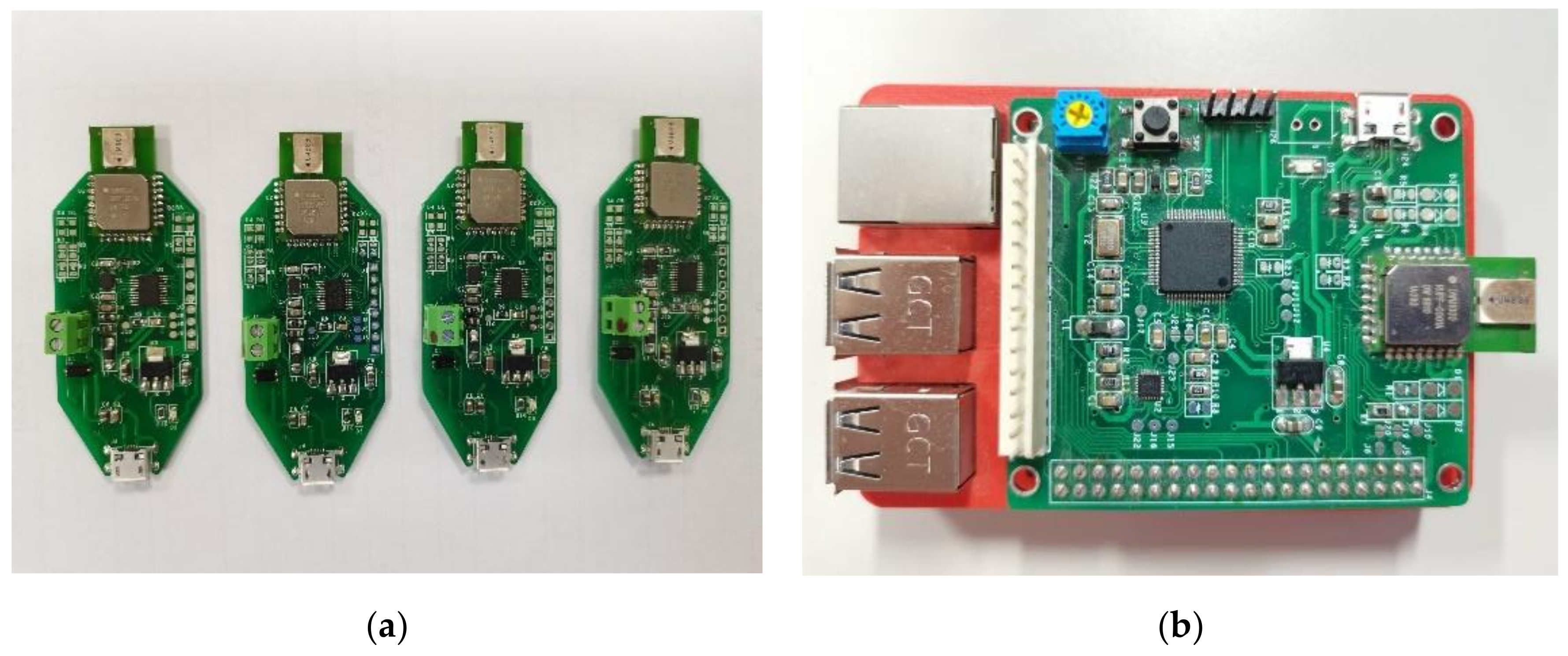
The indoor positioning system utilized in this paper was implemented using UWB sensors DecaWave DWM1000 [39], with an optional frequency band range from 3.5 to 6.5 GHz. The data transmission rates included 110 kbps, 850 kbps, and 6.8 Mbps. The anchor was implemented as in Figure 1a using an STM32F0 microcontroller unit (MCU) with the main frequency of 48 MHz and a UWB sensor DWM1000. The mobile node was implemented as in Figure 1b, combining an STM32F4 MCU with the main frequency of 168 MHz, an IMU MPU 9250, and a UWB sensor DWM1000. An embedded system made with a Raspberry Pi 3 was utilized in the mobile node for positioning calculation and the implementation of EKF to improve positioning results. The sampling frequency for positioning was set as 100 Hz.
The positioning of the mobile node was based on measuring the distance between the mobile node and every anchor. The distance measurement relied on the TOF of the radio between the transmitter and the receiver. Two-way radio transmission and receiving were conducted between both sensors. The mobile node was designated as an initiator that initiates the two-way radio communication, while the anchor was set as a responder. The initiator transmits a message through radio to the responder and records the timestamp of transmission. As the responder receives the message, it sends the same message back to the initiator after a preset time delay. The initiator gets the message and records the timestamp of receiving. The TOF is calculated based on the timestamps of transmission and receiving, and the preset time delays at both the responder and the initiator. The calculation of TOF is affected by the clock drift, frequency drift, fading, shadowing, multi-path propagation, etc. Although more delicate ranging methods such as the asymmetric double-sided two-way-ranging (TWR) method [39] or the TWR method integrated with neural network model [40] have been proposed, noise in the measurement of TOF is unavoidable. Let and be the ideal TOF and the measured TOF, respectively, and be the noise in TOF measurement. Then,
The measured distance between the mobile node and the anchor is calculated as
where c is the speed of radio wave, r is the ideal distance between the mobile node and the anchor, and is the noise of measured distance due to the noise of TOF, . The noise in (2) is usually modeled as an independent and identical distributed (i.i.d.) random variable. The distribution of the noise is usually modeled as the Gaussian distribution [41,42] if the mobile node and the anchor are in the LOS condition. The Gaussian distribution is parameterized with the mean and the variance , i.e., . The noise modeled in the LOS condition is mainly for the environment that no obstacles are placed to block the radio propagation between the mobile node and the corresponding anchor.
The distribution of the noise is modeled as the skew-t distribution [43] for the NLOS condition. The skew-t distribution is parameterized by its location parameter , spread parameter , shape parameter , and degree of freedom . The probability density function (PDF) of the skew-t distribution for the random variable z is defined as
where denotes the PDF of Student’s t-distribution defined as follows:
Note that in (4) denotes the Gamma function. The function in (3) denotes the cumulative distribution function (CDF) of Student’s t-distribution and the random variable in B is defined as:
Therefore, the distance measurement noise for the NLOS condition where skew t-distribution is defined in (3). The noise modeled in the NLOS condition is mainly for the environment that obstacles are placed between the mobile node and the anchor so that the LOS radio propagation is blocked. The radio multi-path propagation due to moving and/or stationary obstacles usually result in the noise modeled in the NLOS condition [44].
3. Mathematical Model of Positioning Errors
3.1. 3D Positioning
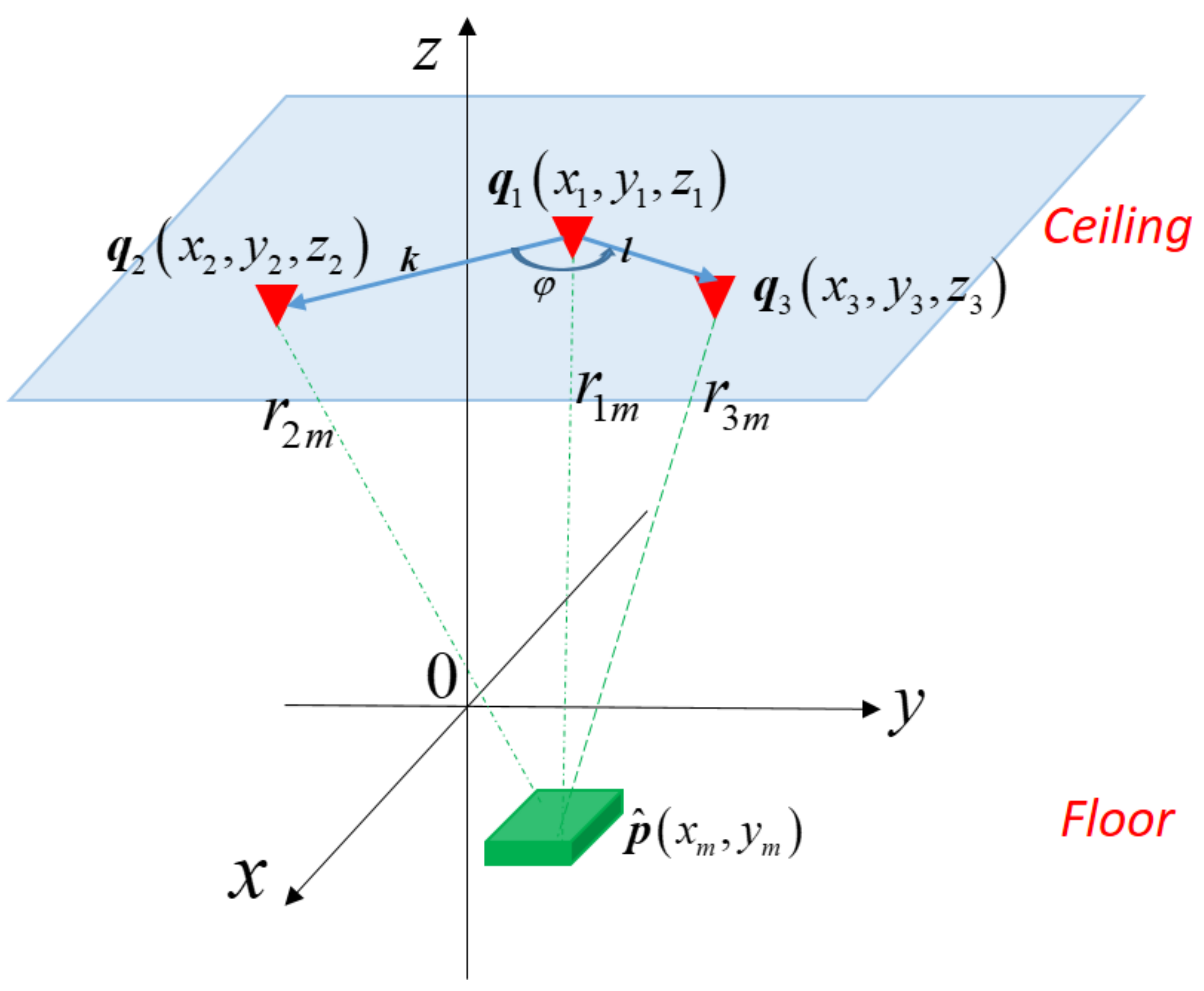
At least four anchors are required for 3D positioning of a mobile node, as shown in Figure 2. Denote as the vector containing the coordinate of the ith anchors, i.e., , i = 1, …,4. The 3D position of the mobile node can be determined by first measuring the distance between the mobile node and every anchor. An EKF is utilized to calculate the position of the mobile node. Denote p and as the vector containing the coordinate the mobile node’s actual 3D position (x, y, z) and measured 3D position , respectively, i.e., and . The measured distance between the mobile node and the ith anchor is calculated as
Similarly, the actual distance between the mobile node and the ith anchor is calculated as
Referring to (2), the measured distance can be represented as
where denotes the measurement noise of the distance between the mobile node and the ith anchor.
Referring to Figure 2, let , , and be the vectors from the position to , to , and , to , respectively. Note that three points at different places form a plane. For the convenience of analysis, let the vectors k and l be on the same plane.
Let , , and , where
With the measured distance defined in (6),
Therefore,
Referring to (13), let
and
Then, (13) is expressed as
where is the measured 3D position of the mobile node, . If H is nonsingular, i.e., det(H) ≠ 0, the measured position of the mobile node can be calculated as
Since , n is perpendicular to the plane formed by three anchor positions . Referring to (14), is calculated under the condition that det(H) ≠ 0. However, , the condition det(H) ≠ 0 results in the condition that m is not perpendicular to the vector n, i.e., m is not on the plane formed by three anchor positions . In other words, the fourth anchor position cannot be on the same plane with in order to have a deterministic position for the mobile node.
Substituting the actual distance between the mobile node to the ith anchor into (12)–(14), the actual position p associated with the actual distance can be theoretically determined similar to the measured position in (17) as
where
Denote as the mobile node’s positioning error,
where . Referring to (14) and (19), is calculated as
Substituting (21) into (20) and going through some derivations yields
where
Referring to (22),
Further derivations in (28) yields
Referring to (29), , and . Therefore,
Referring to (30), implies that . Similarly, and . Therefore, (30) can be further written as
Substituting (31) into (29) yields
Taking the expectation for both sides of (32),
Because , and , , , and , where , and are the angles between vectors and , and , and , respectively, as shown in Figure 2. The inequality in (33) can be rewritten as
It follows that
Because and , , where is the angle between and the normal vector of the plane containing the three anchors , , and . It follows that
in (36) is the variance of the mobile node’s 3D positioning error. The bound for in (36) applies for both the LOS and NLOS conditions. Note that , , and in (36). Given that the distance between pairs of anchors, , , and are decided, (36) suggests that arranging the anchor installation positions with 90° and 0° leads to reasonably small positioning. Moreover, installing the anchors as separated as possible, i.e., k, l, and m being as large as possible, results in reasonably small 3D positioning errors. Note that anchors should be installed at the positions so that k, l, and m are as large as possible, provided that the radio receiving intensity between the mobile node and the anchor is within the rated range.
3.2. 2D Positioning
Essentially, the mathematical model of 2D positioning error is a special case of the one of 3D positioning error. It takes at least three anchors to determine the 2D position of a mobile node. Denote as the vector containing the coordinate of the ith anchors, i.e., , i = 1, …, 3. Referring to Figure 3, let and be the vectors from the position to and to , respectively. Compared with Figure 2, the fourth anchor in Figure 2 is not needed for 2D positioning as shown in Figure 3. Denote p′ and as the vector containing the 2D coordinate the mobile node’s actual position (x, y) and measured position , respectively, i.e., and . Most of the mathematical analysis for 3D positioning in the previous subsection can be used for the analysis of 2D positioning, except that z = 0 and .
Setting in (12) yields
Therefore,
Referring to (38), let
and
Then, (38) is expressed as
If H′ is nonsingular, i.e., det(H′) ≠ 0, the measured position of the mobile node is calculated as
Referring to (42), has a deterministic solution under the condition that det(H′) ≠ 0. Referring to (40), let and . If is the angle between vectors and , . Note that k′ and l′ are the projection of k and l onto the X-Y plane, respectively, as shown in Figure 4a,b. Therefore, has a deterministic solution provided that , i.e., k′ is not parallel with l′.
Referring to (18), the actual position p′ of the mobile node can be theoretically determined similar to the measured position in (42) as
where
Denote as the mobile node’s positioning error,
where and
Substituting (46) into (45) and performing some derivations yields
where , and are as shown in (25) and (26), respectively. Then,
Referring to (48), . Therefore,
Since , it implies that . The inequality (49) can be further written as
Substituting (50) into (48) yields
Taking the expectation for both sides of (51),
It can be further simplified as
Similar to the 3D position error, the variance of the mobile node’s 2D positioning error in (53) also applies for both the LOS and NLOS conditions. Given that the distance between pairs of anchors and are decided, (53) suggests that arranging the anchor positions with 90° leads to reasonably small positioning errors. Moreover, installing the anchors as separated as possible, i.e., k′ and l′ being as large as possible, results in reasonably small 2D positioning errors.
4. Computer Simulations
Computer simulations were implemented to simulate the mobile node’s 2D and 3D positioning. The mobile node was designed to move following a 2D and 3D straight line in a 2D and 3D environment, respectively. A total of 8000 positioning samples were calculated in 2D or 3D simulations, respectively. In other words, the sampling frequency was designed as 100 Hz and 80 s of positioning errors were calculated and recorded for 2D and 3D simulations. The RMSPE was calculated based on the N samples calculated and recorded at the mobile node. Denote as the RMSPE and as the ith sample of positioning error, i = 1, …, N. Then,
where N = 8000. The mobile node’s RMSPE defined in (54) is utilized for the simulation.
Both the LOS and NLOS conditions are to be simulated. The distance measurement noise for the LOS condition and for the NLOS condition. The parameters of the Gaussian distribution for the LOS condition are set as the mean and the standard deviation . The parameters of the skew t-distribution for the NLOS condition are set as , , , and . The variance of 3D position errors defined in (36) can be further simplified if the distance measurement noise . The terms , , and in (36) can be replaced with , , and for the LOS condition. Similarly, the terms and in the variance of 2D position errors defined in (53) can also be replaced with and for the LOS condition.
4.1. 2D positioning Simulation
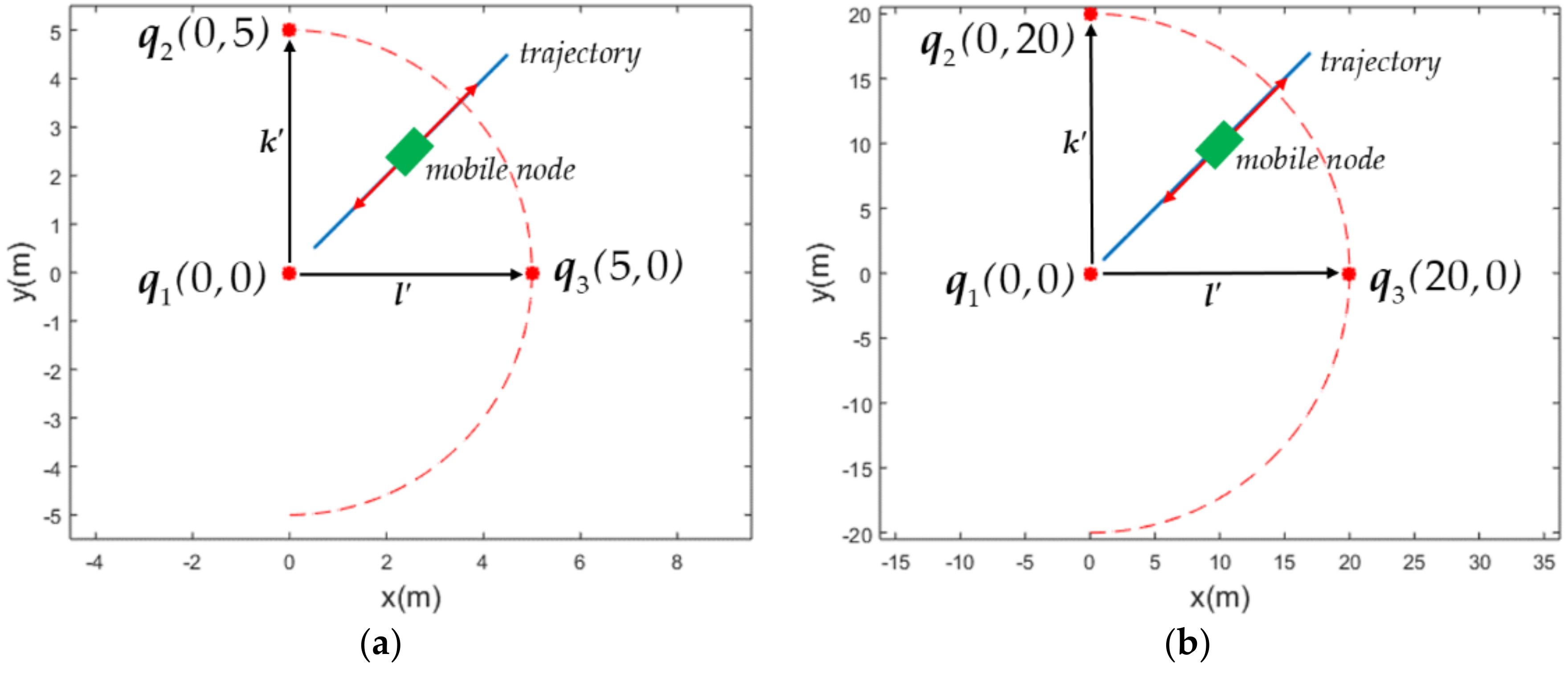
In order to simulate the variation of with respect to the angle between the vectors k’ and l’, the projection of installation positions of three anchors onto the X-Y plane are shown in Figure 4a,b, respectively, for the convenience of illustration. Both Figure 4a,b are essentially similar except that the sizes of the simulation environment are different. As shown in Figure 4a,b, 2 anchors and were installed at fixed positions (0m, 0m) and (0m, 5m), and (0m, 0m) and (0m, 20m), respectively. The mobile node moves from (0.5m, 0.5m) to (4.5m, 4.5m) in Figure 4a and from (2m, 2m) to (18m, 18m) in Figure 4b for four round trips. The anchor was simulated to be installed at different positions on the circumference with a radius of 5m and 20m, respectively, in Figure 4a,b, but both centered at (0m, 0m). The angle ranged from to as in Figure 4a,b. The heights of on the z-axis were assumed to be 4m, 4.2m, and 4.1m, respectively.
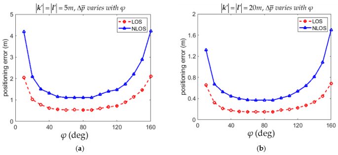
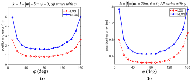
The RMSPE defined in (54) with different angles of for the LOS and NLOS conditions are listed in Table 1 and Table 2, respectively. It is shown in Table 1 that was minimum if = 90° in both 5m × 5m and of 20m × 20m environments for the LOS condition. Table 2 shows that was minimum if = 70° in both 5m × 5m and of 20m × 20m environments for the NLOS condition. However, with = 90° in both 5m × 5m and of 20m × 20m environments were very close to the minimum values occurring at = 70°. The variations of with the angle for the LOS and NLOS conditions in both Table 1 and Table 2 are illustrated in Figure 5a,b, respectively. The suggestion based on (53) that the anchor installation arrangement with = 90° leads to reasonably small positioning error for both the LOS and NLOS conditions is thus justified from both Table 1 and Table 2.
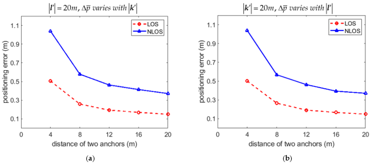
The 2D RMSPE is also affected by the anchor distances . The variation of with different for the LOS and NLOS conditions are calculated in Table 3 and Table 4, respectively. Both Table 3 and Table 4 show that the 2D RMSPE decreased as and/or increased for both the LOS and NLOS conditions. The variations of with anchor distances for the LOS and NLOS conditions are also illustrated in Figure 6a,b, respectively. The suggestion based on (53) that installing the anchors as separated as possible results in reasonably small positioning error is thus justified.
Since the installation arrangement of anchors suggested in this paper was based on the upper bound of the variance of positioning errors in (53), the accuracy of the upper bound is worth evaluation. Denote the upper bound of variance in (53) for the ith sample as , then
where and are the parameters and corresponding to the ith sample data. Denote as the upper bound of average positioning error based on (53) for all N samples, then
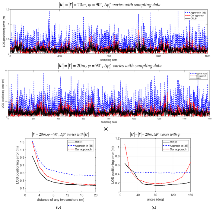
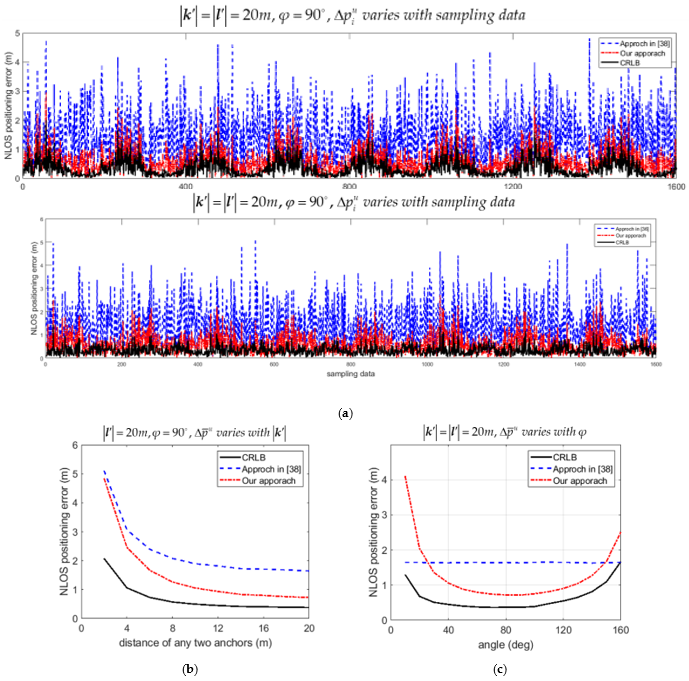
The upper bound of average positioning error in (56) was compared with the one proposed in [38]. The theoretical Cramer-Rao lower bound (CRLB) was also calculated and plotted for comparison. Let the upper bound of positioning error for the ith data . The variations of with samples estimated by our approach and by the approach in [38] are compared in Figure 7a and Figure 8a for the LOS and NLOS condition, respectively. Recall that 8000 samples were recorded in the simulation. Only 20 percent of recorded data are plotted in Figure 7a and Figure 8a for convenience of illustration. Both Figure 7a and Figure 8a show that the upper bound of positioning error was much lower than the ones calculated by the approach in [38], and much closer to the CRLB for the LOS and NLOS conditions, respectively. The variations of upper bound of average positioning error with for the situation that = 20m and = were also compared as in Figure 7b and Figure 8b for the LOS and NLOS conditions, respectively. Figure 7c and Figure 8c show the comparison of with if = = 20m for the LOS and NLOS conditions, respectively. It is shown in Figure 7b,c and Figure 8b,c that was much lower than the one calculated by the approach in [38], and much closer to the CRLB for both the LOS and NLOS conditions.
4.2. 3D Positioning Simulation
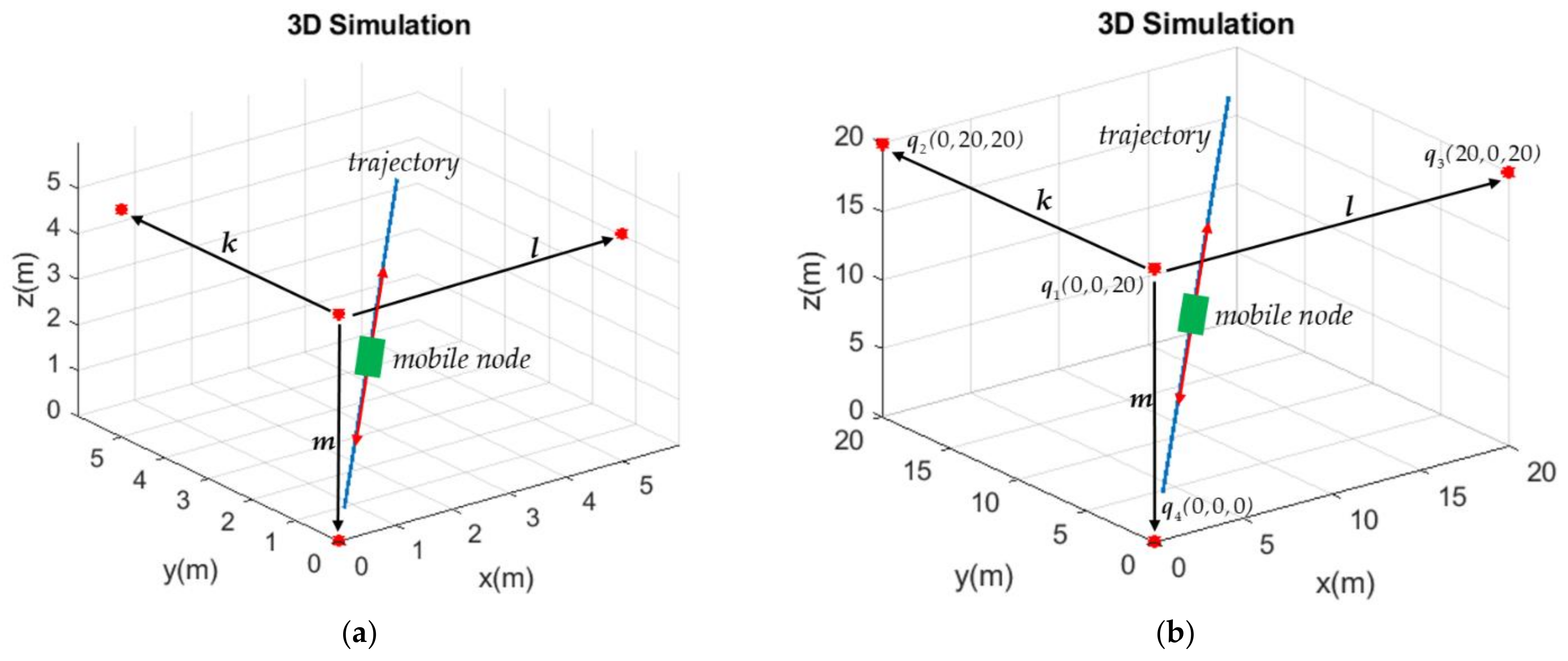
The mobile node’s positioning error defined in (22) was utilized for the 3D simulation. In order to simulate the variations of with respect to the angles between the vectors k and l and the angle between the vectors m and n, the anchors , , and were assumed to be installed in a smaller environment 5m × 5m × 5m and a larger environment 20m × 20m × 20m, as shown in Figure 9a,b, respectively. The mobile node moves from (0.5m, 0.5m, 0.5m) to (4.5m, 4.5 m, 4.5m) in Figure 9a and from (2m, 2m, 2m) to (18m, 18m, 18m) in Figure 9b for four round trips. The anchor and were both simulated to be installed at different positions on the circumference with a radius of 5m and 20m, respectively, in Figure 9a,b, but both centered at the position of providing that other anchors were fixed at the positions shown in Figure 9a,b. The positioning errors were calculated with angles and varying from to . Note that varies by changing the angle between the vectors k and l while varies by changing the angle between the vectors m and n.
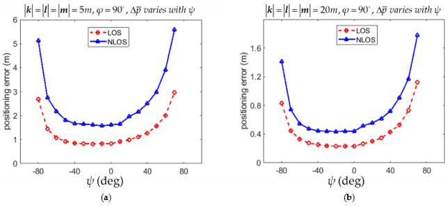
The RMSPE defined in (54) with different angles of for the LOS and NLOS conditions are listed in Table 5 and Table 6, respectively. It is shown in Table 5 that was minimum at = 80° in the 5m × 5m × 5m environment while was minimum at = 70° in the 20m × 20m × 20m environment for the LOS condition. However, with = 90° in both 5m × 5m × 5m and 20m × 20m × 20m environments were very close to the minimum values occurring at = 80° and 70° in the 5m × 5m × 5m and 20m × 20m × 20m environment, respectively. Table 6 shows that was minimum = 90° in both 5m × 5m × 5m and 20m × 20m × 20m environments for the NLOS condition. The variations of with the angle for the LOS and NLOS conditions in both Table 5 and Table 6 are illustrated in Figure 10a,b, respectively. As for the angle , it is shown in Table 7 that was minimum is minimum at = 20° in both 5m × 5m × 5m and 20m × 20m × 20m environments for the LOS condition. However, with = 0° in both 5m × 5m × 5m and 20m × 20m × 20m environments were also very close to the minimum values occurring at = 20° in both environments. It is shown in Table 8 that was minimum at = 10° in the 5m × 5m × 5m environment while was minimum at = 20° in the 20m × 20m × 20m environment for the NLOS condition. However, with = 0° in both 5m × 5m × 5m and 20m × 20m × 20m environments were very close to the minimum values occurring at = 10° and 20° in the 5m × 5m × 5m and 20m × 20m × 20m environment, respectively. The variations of with the angle for the LOS and NLOS conditions in both Table 7 and Table 8 are illustrated in Figure 11a and Figure 11b, respectively. The suggestion based on (36) that the anchor installation arrangement with = 90° and = 0° leads to reasonably small positioning errors for both the LOS and NLOS conditions is thus justified from Table 5, Table 6, Table 7 and Table 8.
5. Experiments
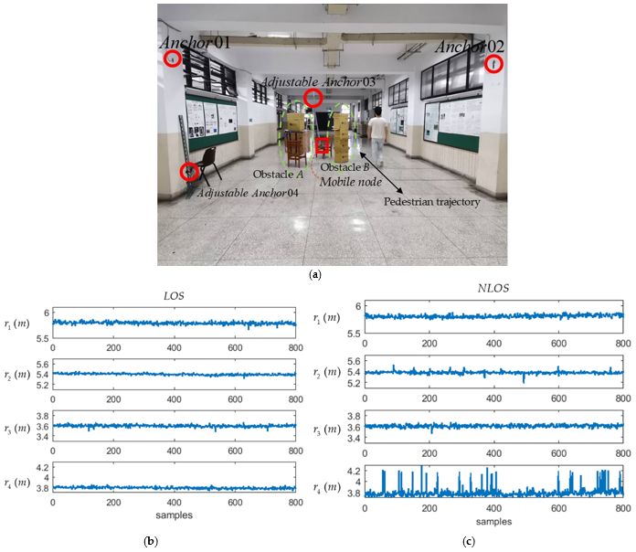
After the computer simulations shown in the previous section, an experiment was conducted to further verify the results obtained in 3D positioning for both the LOS and NLOS conditions. The 3D positioning experiment for the LOS condition was conducted in the environment where no obstacle was placed between the mobile node and every anchor. The experiment was implemented in a corridor outside of the laboratory in an environment 6m × 6m × 3.6m. The installation positions of the four anchors are shown in Figure 12a, where anchors and were installed on the wall with fixed positions. In contrast, the positions of and are adjustable for the positioning evaluations with different angles and . The mobile node moves in the experiment environment with 0.52m above the ground. The illustration of the experiment environment and the moving trajectories of adjustable anchors and are shown in Figure 12b. The mobile node calculates the 3D positioning with EKF [45] and records the positions with a sampling frequency of 100 Hz. The RMSPEs were calculated for every 600 samples.
In the first LOS experiment, the anchors and were installed at the positions with coordinates and respectively, as shown in Figure 12b. It resulted in being equal to 5.79m. The installation positions of anchors were adjusted following the trajectory shown in Figure 12b with varying from 10° to 90°. Note that the z coordinate of was kept constant, 2.52m, while changing the installation positions. Therefore, 5.79m. The installation position of was also adjusted following the trajectory shown in Figure 12b with varying from 0° to 65°. It is shown in Figure 12b that remained a constant, 2.49m, while changed from 0° to 65°. The mobile node was parked at the position to measure the mobile node’s 3D position for different anchor positions. The RMSPEs were calculated with varying from 10° to 90° and yet was set to be 0°. Similarly, the RMSPEs were calculated with ranging from 0° to 65° and yet was set to be 90°. The RMSPEs corresponding to different combinations of and are shown in Table 9. Table 9 shows that was minimum if the installation position of is adjusted so that = 90° under the condition = 0°; or if the installation of is adjusted so that = 0° under the condition = 90°.
In the second LOS experiment, the mobile node was still parked at the position , and both and were set at the position so that = 90° and = 0°. The RMSPEs were measured and calculated while changing both and from 1.79m to 5.79m, and changing from 1.19m to 2.19m. Note that was calculated by changing only one length of vector at a time with the lengths of two other vectors remaining constants. The experiment results are shown in Table 10. Table 10 shows that the decreased if the lengths of 3 vectors , , and were appropriately increased.
The 3D positioning experiment for the NLOS condition was conducted in the same environment as in the LOS experiment, except that several stationary and moving obstacles were placed between the mobile node and the anchors. Figure 13a shows that a stationary obstacle A with the dimension 0.7m × 0.4m × 1.65m was placed between the mobile node and the anchor while a stationary obstacle B with the dimension 0.6m × 0.25m × 1.65m was placed between the mobile node and the anchor . In addition to the stationary obstacles, a pedestrian was arranged to walk back and forth following a straight line between the mobile node and the anchor shown in Figure 13a. The measured distance between the mobile node and every ith anchor , i = 1, …, 4, for the LOS and NLOS conditions are compared in Figure 13b and Figure 13c, respectively. From the measured distances compared in Figure 13b,c, it is shown that both stationary and moving obstacles did affect the distance measurement. The same 3D positioning experiment for the NLOS condition was conducted as for the LOS condition. The RMSPEs corresponding to different combinations of and for the NLOS condition are shown in Table 11. Table 11 shows that was minimum if the installation position of is adjusted so that = 90° under the condition = 0°. The RMSPE was also minimum if the installation of is adjusted so that = 0° under the condition = 90°. The RMSPEs were calculated by changing only one vector length at a time with the lengths of two other vectors remaining constants. The experiment results are shown in Table 12. Table 12 shows that the decreased if the lengths of three vectors , , and were appropriately increased.
The suggestion based on (36) that the anchor installation arrangement with = 90° and = 0° leads to reasonably small 3D positioning errors for both the LOS and NLOS conditions is thus justified from the experimental results in Table 9 and Table 11. Moreover, the suggestion that installing the anchors as separated as possible leads to reasonably small 3D positioning errors is also justified from the experimental results in Table 10 and Table 12.
6. Conclusions
The upper bounds of variance of both 2D and 3D positioning errors were derived in this paper. The mathematical model for the variance of positioning errors shed light on some tips regarding installation positions of anchors. The positioning errors can be reduced through an appropriate arrangement of anchors’ installation positions according to the mathematical model derived in the paper. Computer simulations and practical experiments were conducted to verify the suggestions of anchor installation positions obtained from the mathematical model.
The positioning accuracy of UWB sensors has attracted a lot of attention lately due to their cost-effective positioning performance. The positioning errors analyzed in the paper were limited to the 2D or 3D positions only. However, the positioning errors can be expanded to include the linear and angular velocities and accelerations if the UWB sensors are combined with the inertial measurement units (IMU). Further works can be performed to derive the mathematical model for the “expanded” positioning errors so that more installation suggestions regarding improving positioning accuracy can be obtained from the model. Further works can also be performed to derive the lower bound of variance of positioning errors based on the proposed mathematical model. The range of positioning errors associated with a combination of anchor installation positions can be estimated with more accuracy if both upper and lower bounds of positioning errors are calculated.
Author Contributions
Conceptualization, L.Y. (Leehter Yao); methodology, L.Y. (Leehter Yao) and Y.-W.W.; software, L.Y. (Lei Yao); validation, L.Y. (Lei Yao); writing—original draft preparation, L.Y. (Lei Yao); writing— review and editing, L.Y. (Leehter Yao); supervision, L.Y. (Leehter Yao); project administration, L.Y. (Leehter Yao); funding acquisition, L.Y. (Leehter Yao). All authors have read and agreed to the published version of the manuscript.
Funding
This research was funded by Ministry of Science and Technology, Taiwan, grant number MOST 107-2221-E-027-086-MY3.
Conflicts of Interest
The authors declare no conflict of interest.
References
- Li, X.; Wang, J.; Liu, C.; Zhang, L.; Li, Z. Integrated wifi/pdr/smartphone using an adaptive system noise extended kalman filter algorithm for indoor localization. ISPRS Int. J. Geo-Inf. 2016, 5, 8. [Google Scholar] [CrossRef] [Green Version]
- Zuin, S.; Calzavara, M.; Sgarbossa, F.; Persona, A. Ultra wide band indoor positioning system: Analysis and testing of an IPS technology. IFAC 2018, 51, 1488–1492. [Google Scholar]
- Mendoza-Silva, G.M.; Torres-Sospedra, J.; Huerta, J. A more realistic error distance calculation for indoor positioning systems accuracy evaluation. In Proceedings of the 2017 International Conference on Indoor Positioning and Indoor Navigation (IPIN), Sapporo, Japan, 18–21 September 2017; pp. 1–8. [Google Scholar]
- Anagnostopoulos, G.G.; Deriaz, M.; Gaspoz, J.; Konstantas, D.; Guessous, I. Navigational needs and requirements of hospital staff: Geneva university hospitals case study. In Proceedings of the 2017 International Conference on Indoor Positioning and Indoor Navigation (IPIN), Sapporo, Japan, 18–21 September 2017; pp. 1–8. [Google Scholar]
- Holm, S. Ultrasound positioning based on time-of-flight and signal strength. In Proceedings of the 2012 International Conference on Indoor Positioning and Indoor Navigation (IPIN), Sydney, NSW, Australia, 13–15 November 2012; pp. 1–6. [Google Scholar]
- Mohebbi, P.; Stroulia, E.; Nikolaidis, I. Sensor-data fusion for multi-person indoor position estimation. Sensors 2017, 17, 2377. [Google Scholar] [CrossRef] [Green Version]
- Castillo-Cara, M.; Lovon-Melgarejo, J.; Bravo-Rocca, G.; Orozco-Barbosa, L.; Garcia-Varea, I. An empirical study of the transmission power setting for Bluetooth-based indoor localization mechanisms. Sensors 2017, 17, 1318. [Google Scholar] [CrossRef] [PubMed] [Green Version]
- Zhou, Y.D.; Wei, M.X.; Zhuang, H. Research on ZigBee indoor technology positioning based on RSSI. Procedia Comput. Sci. 2019, 154, 424–429. [Google Scholar]
- Diallo, A.; Lu, Z.; Zhao, X. Wireless indoor localization using passive RFID tags. Procedia Comput. Sci. 2019, 155, 210–217. [Google Scholar] [CrossRef]
- Xiao, W.; Ni, W.; Toh, Y.K. Integrated Wi-Fi fingerprinting and inertial sensing for indoor positioning. In Proceedings of the 2011 International Conference on Indoor Positioning and Indoor Navigation (IPIN), Guimaraes, Portugal, 21–23 September 2011; pp. 1–6. [Google Scholar]
- Jiménez Ruiz, A.R.; Seco Granja, F. Comparing Ubisense, BeSpoon, and DecaWave UWB position systems: Indoor performance analysis. IEEE Trans. Instrum. Meas. 2017, 66, 2106–2117. [Google Scholar] [CrossRef]
- Park, H.; Noh, J.; Cho, S. Three-dimensional positioning system using Bluetooth low-energy beacons. IJDSN 2016, 12. [Google Scholar] [CrossRef] [Green Version]
- He, Y.; Bilgic, A. Iterative least squares method for global positioning system. Adv. Radio Sci. 2011, 9, 203–208. [Google Scholar] [CrossRef] [Green Version]
- Khalaf-Allah, M. Particle filtering for three-dimensional TDoA-based positioning using four anchor nodes. Sensors 2020, 20, 4516. [Google Scholar] [CrossRef]
- Yao, L.; Wu, Y.A.; Yao, L.; Liao, Z.Z. An integrated IMU and UWB sensor based indoor positioning system. In Proceedings of the 2017 International Conference on Indoor Positioning and Indoor Navigation (IPIN), Sapporo, Japan, 18–21 September 2017; pp. 1–8. [Google Scholar]
- Zeng, Z.; Liu, S.; Wang, L. UWB/IMU integration approach with NLOS identification and mitigation. In Proceedings of the 2018 52nd Annual Conference on Information Sciences and Systems (CISS), Princeton, NJ, USA, 21–23 March 2018; pp. 1–6. [Google Scholar]
- Zeng, Z.; Liu, S.; Wang, L. NLOS detection and mitigation for UWB/IMU fusion system based on EKF and CIR. In Proceedings of the 2018 IEEE 18th International Conference on Communication Technology (ICCT), Chongqing, China, 8–11 October 2018; pp. 376–381. [Google Scholar]
- Liu, F.; Li, X.; Wang, J.; Zhang, J. An adaptive UWB/MEMS-IMU complementary Kalman filter for indoor position in NLOS environment. Remote Sens. 2019, 11, 2628. [Google Scholar] [CrossRef] [Green Version]
- Li, Z.; Chang, G.; Gao, J.; Wang, J.; Hernandez, A. GPS/UWB/MEMS-IMU tightly coupled navigation with improved robust Kalman filter. Adv. Space Res. 2016, 58, 2424–2434. [Google Scholar] [CrossRef]
- Fan, Q.; Sun, B.; Sun, Y.; Zhuang, X. Performance enhancement of MEMS-based INS/UWB integration for indoor navigation applications. IEEE Sens. J. 2017, 17, 3116–3130. [Google Scholar] [CrossRef]
- Nakamura, S.; Higashi, Y.; Masuda, A.; Miura, N. A positioning system and position control system of a quad-rotor applying Kalman filter to a UWB module and an IMU. In Proceedings of the 2020 IEEE/SICE International Symposium on System Integration (SII), Honolulu, HI, USA, 12–15 January 2020; pp. 747–752. [Google Scholar]
- Jachimczyk, B.; Dziak, D.; Kulesza, W.J. Customization of UWB 3D-RTLS based on the new uncertainty model of the AoA ranging technique. Sensors 2017, 17, 227. [Google Scholar] [CrossRef] [Green Version]
- Ferreira, A.G.; Fernandes, D.; Catarino, A.P.; Monteiro, J.L. Performance analysis of ToA-based positioning algorithms for static and dynamic targets with low ranging measurements. Sensors 2017, 17, 1915. [Google Scholar] [CrossRef]
- Zhang, K.; Shen, C.; Zhou, Q.; Wang, H.; Gao, Q.; Chen, Y. A combined GPS UWB and MARG position algorithm for indoor and outdoor mixed scenario. Clust. Comput. 2019, 22, 5965–5974. [Google Scholar] [CrossRef]
- Ding, G.; Lu, H.; Bai, J.; Qin, X. Development of a high precision UWB/Vision-based AGV and control system. In Proceedings of the 2020 5th International Conference on Control and Robotics Engineering (ICCRE), Osaka, Japan, 24–26 April 2020; pp. 99–103. [Google Scholar]
- Song, Y.; Guan, M.; Tay, W.P.; Law, C.L.; Wen, C. UWB/LiDAR fusion for cooperative range-only SLAM. In Proceedings of the 2019 International Conference on Robotics and Automation (ICRA), Montreal, QC, Canada, 20–24 May 2019; pp. 6568–6574. [Google Scholar]
- Renaudin, V.; Susi, M.; Lachapelle, G. Step length estimation using handheld inertial sensors. Sensors 2012, 12, 8507–8525. [Google Scholar] [CrossRef]
- Song, Y.; Hsu, L.T. Tightly coupled integrated navigation system via factor graph for UAV indoor localization. Aerosp. Sci. Technol. 2021, 108. [Google Scholar] [CrossRef]
- Wen, K.; Yu, K.; Li, Y.; Zhang, S.; Zhang, W. A new quaternion Kalman filter based foot-mounted IMU and UWB tightly-coupled method for indoor pedestrian navigation. IEEE Trans. Veh. Tech. 2020, 69, 4340–4352. [Google Scholar] [CrossRef]
- Hol, J.D.; Dijkstra, F.; Luinge, H.; Schon, T.B. Tightly coupled UWB/IMU pose estimation. In Proceedings of the 2009 IEEE International Conference on Ultra-Wideband, Vancouver, BC, Canada, 9–11 September 2009; pp. 688–692. [Google Scholar]
- Li, X.; Wang, Y.; Khoshelham, K. A robust and adaptive complementary Kalman filter based on mahalanobis distance for ultra wideband/inertial measurement unit fusion positioning. Sensors 2018, 18, 3435. [Google Scholar] [CrossRef] [Green Version]
- Liu, J.; Pu, J.; Sun, L.; He, Z. An approach to robust INS/UWB integrated positioning for autonomous indoor mobile robots. Sensors 2019, 19, 950. [Google Scholar] [CrossRef] [Green Version]
- Shen, Y.; Win, M.Z. Fundamental limits of wideband localization— Part I: A general framework. IEEE Trans. Inf. Theory 2010, 56, 4956–4980. [Google Scholar] [CrossRef]
- Miraglia, G.; Maleki, K.N.; Hook, L.R. Comparison of two sensor data fusion methods in a tightly coupled UWB/IMU 3-D localization system. In Proceedings of the 2017 International Conference on Engineering, Technology and Innovation (ICE/ITMC), Madeira, Portugal, 27–29 June 2017; pp. 611–618. [Google Scholar]
- Xu, Y.; Shmaliy, Y.S.; Chen, X.; Li, Y.; Ma, W. Robust inertial navigation system/ultra wide band integrated indoor quadrotor localization employing adaptive interacting multiple model-unbiased finite impulse response/Kalman filter estimator. Aerosp. Sci. Technol. 2020, 98, 105683. [Google Scholar] [CrossRef]
- Zhang, R.; Shen, F.; Liang, Y.; Zhao, D. Using UWB aided GNSS/INS integrated navigation to bridge GNSS outages based on optimal anchor distribution strategy. In Proceedings of the 2020 IEEE/ION Position, Location and Navigation Symposium (PLANS), Portland, OR, USA, 20–23 April 2020; pp. 1405–1411. [Google Scholar]
- Tahsin, M.; Sultana, S.; Reza, T.; Hossam-E-Haider, M. Analysis of DOP and its preciseness in GNSS position estimation. In Proceedings of the 2015 International Conference on Electrical Engineering and Information Communication Technology (ICEEICT), Savar, Bangladesh, 21–23 May 2015; pp. 1–6. [Google Scholar]
- Monica, S.; Ferrari, G. UWB-based localization in large indoor scenarios: Optimized placement of anchor nodes. IEEE Trans. Aerosp. Electron. Syst. 2015, 51, 987–999. [Google Scholar] [CrossRef]
- Decawave. The Implementation of Two-Way Ranging with the DW 1000; Version 2.2; DecaWave Limited: Dublin, Ireland, 2015. [Google Scholar]
- Peter, K.; Matjaž, V.; Marko, M. Distance measurements in UWB-radio localization systems corrected with a feedforward neural network model. Sensors 2021, 21, 2294. [Google Scholar]
- Larsson, E.G. Cram’er-Rao bound analysis of distribution positioning in sensor networks. IEEE Trans. Signal Process. Lett. 2004, 11, 334–337. [Google Scholar] [CrossRef]
- Qi, Y.; Kobayashi, H.; Suda, H. Analysis of wireless geolocation in a non-line-of-sight environment. IEEE Trans. Wireless Commun. 2006, 5, 672–681. [Google Scholar]
- Nurminen, H.; Ardeshiri, T.; Piché, R.; Gustafsson, F.A. NLOS-robust TOA positioning filter based on a skew-t measurement noise model. In Proceedings of the 2015 International Conference on Indoor Positioning and Indoor Navigation (IPIN), Banff, AB, Canada, 13–16 October 2015; pp. 1–7. [Google Scholar]
- Shen, Y.; Wymeersch, H.; Win, M.Z. Fundamental limits of wideband localization- part II: Cooperative networks. IEEE Trans. Inf. Theory 2010, 56, 4981–5000. [Google Scholar] [CrossRef] [Green Version]
- Khan, R.; Khan, S.U.; Khan, S.; Khan, M.U.A. Localization performance evaluation of extended kalman filter in wireless sensors network. Procedia Comput. Sci. 2014, 32, 117–124. [Google Scholar] [CrossRef] [Green Version]
Figure 1.
The UWB sensors used in this paper. (a) anchors; (b) mobile node.

Figure 2.
Positioning of a mobile node in a 3D space with 4 anchors.

Figure 3.
Positioning of a mobile node in a 2D space with three anchors.

Figure 4.
Projection of installation positions of anchors onto the X−Y plane and the moving trajectory of the mobile node. (a) The environment of 5m × 5m. (b) The environment of 20m × 20m.
Figure 4.
Projection of installation positions of anchors onto the X−Y plane and the moving trajectory of the mobile node. (a) The environment of 5m × 5m. (b) The environment of 20m × 20m.

Figure 5.
Variation of 2D RMSPE with angles for the LOS and NLOS conditions. (a) The environment of 5m × 5m. (b) The environment of 20m × 20m.
Figure 5.
Variation of 2D RMSPE with angles for the LOS and NLOS conditions. (a) The environment of 5m × 5m. (b) The environment of 20m × 20m.

Figure 6.
Variation of 2D RMSPE with different anchor distances and . (a) Variation of with provided that ; (b) Variation of with provided that .
Figure 6.
Variation of 2D RMSPE with different anchor distances and . (a) Variation of with provided that ; (b) Variation of with provided that .

Figure 7.
Comparison of upper bound of 2D positioning errors estimated by our approach and the approach in [38] for the LOS condition. (a) Variation of with samples; (b) Variation of with distance ; (c) Variation of with angle .
Figure 7.
Comparison of upper bound of 2D positioning errors estimated by our approach and the approach in [38] for the LOS condition. (a) Variation of with samples; (b) Variation of with distance ; (c) Variation of with angle .

Figure 8.
Comparison of upper bound of 2D positioning errors estimated by our approach and the approach in [38] for the NLOS condition. (a) Variation of with samples; (b) Variation of with distance ; (c) Variation of with angle .
Figure 8.
Comparison of upper bound of 2D positioning errors estimated by our approach and the approach in [38] for the NLOS condition. (a) Variation of with samples; (b) Variation of with distance ; (c) Variation of with angle .

Figure 9.
Installation positions of anchors and moving trajectory of the mobile node. (a) The environment of 5m × 5m × 5m. (b) The environment of 20m × 20m × 20m.
Figure 9.
Installation positions of anchors and moving trajectory of the mobile node. (a) The environment of 5m × 5m × 5m. (b) The environment of 20m × 20m × 20m.

Figure 10.
Variation of 3D RMSPE with angles for the LOS and NLOS conditions. (a) The environment of 5m × 5m × 5m. (b) The environment of 20m × 20m × 20m.
Figure 10.
Variation of 3D RMSPE with angles for the LOS and NLOS conditions. (a) The environment of 5m × 5m × 5m. (b) The environment of 20m × 20m × 20m.

Figure 11.
Variation of 3D RMSPE with angles for the LOS and NLOS conditions. (a) The environment of 5m × 5m × 5m. (b) The environment of 20m × 20m × 20m.
Figure 11.
Variation of 3D RMSPE with angles for the LOS and NLOS conditions. (a) The environment of 5m × 5m × 5m. (b) The environment of 20m × 20m × 20m.

Figure 12.
Experiment of measuring mobile node’s positioning errors. (a) Photograph showing the positions of the four anchors and the mobile node for the LOS condition; (b) Illustration of the experimental environment and the moving trajectory of the adjustable anchors.
Figure 12.
Experiment of measuring mobile node’s positioning errors. (a) Photograph showing the positions of the four anchors and the mobile node for the LOS condition; (b) Illustration of the experimental environment and the moving trajectory of the adjustable anchors.

Figure 13.
Experiment of measuring the mobile node’s positioning errors. (a) Photograph showing the positions of the four anchors and obstacles; (b) Measured distances between the mobile node and four anchors for the LOS condition; (c) Measured distances between the mobile node and four anchors for the NLOS condition.


Table 1.
The 2D RMSPE (m) with varying in the 5m × 5m and 20m × 20m environments for the LOS condition.
Table 1.
The 2D RMSPE (m) with varying in the 5m × 5m and 20m × 20m environments for the LOS condition.
| 10 | 20 | 30 | 40 | 50 | 60 | 70 | 80 | 90 | 100 | 110 | 120 | 130 | 140 | 150 | 160 | |
|---|---|---|---|---|---|---|---|---|---|---|---|---|---|---|---|---|
| 5m × 5m | 2.044 | 1.022 | 0.783 | 0.620 | 0.556 | 0.539 | 0.540 | 0.536 | 0.526 | 0.606 | 0.677 | 0.723 | 0.891 | 1.148 | 1.458 | 2.104 |
| 20m × 20m | 0.654 | 0.325 | 0.213 | 0.176 | 0.155 | 0.150 | 0.150 | 0.149 | 0.149 | 0.184 | 0.195 | 0.227 | 0.270 | 0.333 | 0.448 | 0.684 |
Table 2.
The 2D RMSPE (m) with varying in the 5m × 5m and 20m × 20m environments for the NLOS condition.
Table 2.
The 2D RMSPE (m) with varying in the 5m × 5m and 20m × 20m environments for the NLOS condition.
| 10 | 20 | 30 | 40 | 50 | 60 | 70 | 80 | 90 | 100 | 110 | 120 | 130 | 140 | 150 | 160 | |
|---|---|---|---|---|---|---|---|---|---|---|---|---|---|---|---|---|
| 5m × 5m | 4.192 | 2.091 | 1.513 | 1.323 | 1.155 | 1.117 | 1.112 | 1.113 | 1.114 | 1.261 | 1.402 | 1.477 | 1.745 | 2.210 | 2.891 | 4.219 |
| 20m × 20m | 1.323 | 0.675 | 0.530 | 0.448 | 0.402 | 0.375 | 0.368 | 0.373 | 0.371 | 0.412 | 0.453 | 0.538 | 0.644 | 0.813 | 1.085 | 1.699 |
Table 3.
The 2D RMSPE (m) with varying anchor distances and for the LOS condition.
| Distances (m) | 4 | 8 | 12 | 16 | 20 |
|---|---|---|---|---|---|
| |k’| (m) | 0.505 | 0.259 | 0.194 | 0.170 | 0.149 |
| |l’| (m) | 0.501 | 0.266 | 0.192 | 0.167 | 0.149 |
Table 4.
The 2D RMSPE (m) with varying anchor distances and for the NLOS condition.
| Distances (m) | 4 | 8 | 12 | 16 | 20 |
|---|---|---|---|---|---|
| |k’| (m) | 1.039 | 0.578 | 0.463 | 0.414 | 0.371 |
| |l’| (m) | 1.040 | 0.568 | 0.463 | 0.394 | 0.371 |
Table 5.
The 3D RMSPE (m) with varying in the 5m × 5m × 5m and 20m × 20m × 20m environments for the LOS condition.
Table 5.
The 3D RMSPE (m) with varying in the 5m × 5m × 5m and 20m × 20m × 20m environments for the LOS condition.
| 10 | 20 | 30 | 40 | 50 | 60 | 70 | 80 | 90 | 100 | 110 | 120 | 130 | 140 | 150 | 160 | |
|---|---|---|---|---|---|---|---|---|---|---|---|---|---|---|---|---|
| (5m)3 | 2.593 | 1.403 | 1.058 | 0.923 | 0.872 | 0.847 | 0.838 | 0.835 | 0.837 | 0.903 | 0.957 | 1.043 | 1.177 | 1.400 | 1.805 | 2.622 |
| (20m)3 | 0.797 | 0.427 | 0.318 | 0.270 | 0.252 | 0.240 | 0.238 | 0.239 | 0.239 | 0.259 | 0.281 | 0.313 | 0.373 | 0.467 | 0.627 | 0.961 |
Table 6.
The 3D RMSPE (m) with varying in the 5m × 5m × 5m and 20m × 20m × 20m environments for the NLOS condition.
Table 6.
The 3D RMSPE (m) with varying in the 5m × 5m × 5m and 20m × 20m × 20m environments for the NLOS condition.
| 10 | 20 | 30 | 40 | 50 | 60 | 70 | 80 | 90 | 100 | 110 | 120 | 130 | 140 | 150 | 160 | |
|---|---|---|---|---|---|---|---|---|---|---|---|---|---|---|---|---|
| (5m)3 | 4.936 | 2.725 | 2.076 | 1.794 | 1.676 | 1.639 | 1.621 | 1.614 | 1.591 | 1.719 | 1.828 | 2.039 | 2.368 | 2.649 | 3.535 | 5.021 |
| (20m)3 | 1.539 | 0.813 | 0.599 | 0.510 | 0.460 | 0.454 | 0.452 | 0.454 | 0.450 | 0.510 | 0.531 | 0.603 | 0.687 | 0.830 | 1.050 | 1.533 |
Table 7.
The 3D RMSPE (m) with varying in the 5m × 5m × 5m and 20m × 20m × 20m environments for the LOS condition.
Table 7.
The 3D RMSPE (m) with varying in the 5m × 5m × 5m and 20m × 20m × 20m environments for the LOS condition.
| 80 | 70 | 60 | 50 | 40 | 30 | 20 | 10 | 0 | −10 | −20 | −30 | −40 | −50 | −60 | −70 | |
|---|---|---|---|---|---|---|---|---|---|---|---|---|---|---|---|---|
| (5m)3 | 2.679 | 1.437 | 1.082 | 0.925 | 0.848 | 0.830 | 0.822 | 0.834 | 0.828 | 0.910 | 0.994 | 1.113 | 1.274 | 1.559 | 2.002 | 2.967 |
| (20m)3 | 0.830 | 0.446 | 0.330 | 0.275 | 0.252 | 0.237 | 0.231 | 0.231 | 0.232 | 0.265 | 0.299 | 0.345 | 0.431 | 0.529 | 0.729 | 1.120 |
Table 8.
The 3D RMSPE (m) with varying in the 5m × 5m × 5m and 20m × 20m × 20m environments for the NLOS condition.
Table 8.
The 3D RMSPE (m) with varying in the 5m × 5m × 5m and 20m × 20m × 20m environments for the NLOS condition.
| 80 | 70 | 60 | 50 | 40 | 30 | 20 | 10 | 0 | −10 | −20 | −30 | −40 | −50 | −60 | −70 | |
|---|---|---|---|---|---|---|---|---|---|---|---|---|---|---|---|---|
| (5m)3 | 5.139 | 2.750 | 2.174 | 1.817 | 1.667 | 1.650 | 1.615 | 1.575 | 1.614 | 1.655 | 1.962 | 2.156 | 2.502 | 2.985 | 3.911 | 5.593 |
| (20m)3 | 1.415 | 0.742 | 0.547 | 0.474 | 0.446 | 0.441 | 0.435 | 0.441 | 0.438 | 0.516 | 0.556 | 0.618 | 0.720 | 0.906 | 1.169 | 1.780 |
Table 9.
The 3D RMSPE with varying angles and for the LOS condition.
| group 1 | 90 | 0 | 0.0743 |
| 70 | 0 | 0.1366 | |
| 55 | 0 | 0.2214 | |
| 40 | 0 | 0.2965 | |
| 25 | 0 | 0.6745 | |
| 10 | 0 | 1.4545 | |
| group 2 | 90 | 0 | 0.0743 |
| 90 | 20 | 0.1404 | |
| 90 | 35 | 0.2136 | |
| 90 | 50 | 0.3018 | |
| 90 | 65 | 0.5648 |
Table 10.
The 3D RMSPE with varying anchor distances , , and for the LOS condition.
| |k| (m) | |l| (m) | |m| (m) | ||
|---|---|---|---|---|
| group 1 | 5.79 | 5.79 | 2.19 | 0.0743 |
| 5.79 | 4.79 | 2.19 | 0.1115 | |
| 5.79 | 3.79 | 2.19 | 0.1218 | |
| 5.79 | 2.79 | 2.19 | 0.1807 | |
| 5.79 | 1.79 | 2.19 | 0.3169 | |
| group 2 | 5.79 | 5.79 | 2.19 | 0.0743 |
| 5.79 | 5.79 | 1.69 | 0.1850 | |
| 5.79 | 5.79 | 1.19 | 0.2852 | |
| group 3 | 5.79 | 5.79 | 2.19 | 0.0743 |
| 4.79 | 5.79 | 2.19 | 0.1239 | |
| 3.79 | 5.79 | 2.19 | 0.1544 | |
| 2.79 | 5.79 | 2.19 | 0.1879 | |
| 1.79 | 5.79 | 2.19 | 0.2989 |
Table 11.
The 3D RMSPE environments for the NLOS condition. and for the NLOS condition.
| group 1 | 90 | 0 | 0.5452 |
| 70 | 0 | 0.6355 | |
| 55 | 0 | 0.6758 | |
| 40 | 0 | 0.9418 | |
| 25 | 0 | 1.6660 | |
| 10 | 0 | 2.9914 | |
| group 2 | 90 | 0 | 0.5452 |
| 90 | 20 | 0.5659 | |
| 90 | 35 | 0.7983 | |
| 90 | 50 | 1.0277 | |
| 90 | 65 | 1.1303 |
Table 12.
The 3D RMSPE with varying anchor distances , , and for the NLOS condition.
| |k| (m) | |l| (m) | |m| (m) | ||
|---|---|---|---|---|
| group 1 | 5.79 | 5.79 | 2.19 | 0.5452 |
| 5.79 | 4.79 | 2.19 | 0.7263 | |
| 5.79 | 3.79 | 2.19 | 0.7575 | |
| 5.79 | 2.79 | 2.19 | 0.8255 | |
| 5.79 | 1.79 | 2.19 | 1.0081 | |
| group 2 | 5.79 | 5.79 | 2.19 | 0.5452 |
| 5.79 | 5.79 | 1.69 | 0.8880 | |
| 5.79 | 5.79 | 1.19 | 1.0658 | |
| group 3 | 5.79 | 5.79 | 2.19 | 0.5452 |
| 4.79 | 5.79 | 2.19 | 0.7302 | |
| 3.79 | 5.79 | 2.19 | 0.7333 | |
| 2.79 | 5.79 | 2.19 | 0.7593 | |
| 1.79 | 5.79 | 2.19 | 0.9898 |
Publisher’s Note: MDPI stays neutral with regard to jurisdictional claims in published maps and institutional affiliations. |
© 2021 by the authors. Licensee MDPI, Basel, Switzerland. This article is an open access article distributed under the terms and conditions of the Creative Commons Attribution (CC BY) license (https://creativecommons.org/licenses/by/4.0/).
Share and Cite
MDPI and ACS Style
Yao, L.; Yao, L.; Wu, Y.-W. Analysis and Improvement of Indoor Positioning Accuracy for UWB Sensors. Sensors 2021, 21, 5731. https://doi.org/10.3390/s21175731
AMA Style
Yao L, Yao L, Wu Y-W. Analysis and Improvement of Indoor Positioning Accuracy for UWB Sensors. Sensors. 2021; 21(17):5731. https://doi.org/10.3390/s21175731
Chicago/Turabian StyleYao, Leehter, Lei Yao, and Yeong-Wei Wu. 2021. "Analysis and Improvement of Indoor Positioning Accuracy for UWB Sensors" Sensors 21, no. 17: 5731. https://doi.org/10.3390/s21175731
Note that from the first issue of 2016, this journal uses article numbers instead of page numbers. See further details here.