A Novel Epidemic Model for Wireless Rechargeable Sensor Network Security


1
School of Mechanical and Electric Engineering, Guangzhou University, Guangzhou 510006, China
2
School of Electronics and Communication Engineering, Guangzhou University, Guangzhou 510006, China
*
Author to whom correspondence should be addressed.
Sensors 2021, 21(1), 123; https://doi.org/10.3390/s21010123
Submission received: 9 November 2020
/
Revised: 22 December 2020
/
Accepted: 23 December 2020
/
Published: 27 December 2020
(This article belongs to the Special Issue Wireless Communication in Internet of Things)
Abstract
:With the development of wireless rechargeable sensor networks (WRSNs ), security issues of WRSNs have attracted more attention from scholars around the world. In this paper, a novel epidemic model, SILS(Susceptible, Infected, Low-energy, Susceptible), considering the removal, charging and reinfection process of WRSNs is proposed. Subsequently, the local and global stabilities of disease-free and epidemic equilibrium points are analyzed and simulated after obtaining the basic reproductive number . Detailedly, the simulations further reveal the unique characteristics of SILS when it tends to being stable, and the relationship between the charging rate and . Furthermore, the attack-defense game between malware and WRSNs is constructed and the optimal strategies of both players are obtained. Consequently, in the case of and , the validity of the optimal strategies is verified by comparing with the non-optimal control group in the evolution of sensor nodes and accumulated cost.
1. Introduction
1.1. Research Background
Wireless sensor networks (WSNs) have attracted researchers’ attention worldwide over the last few years. WSNs consist of sensor nodes that have data storing and data transmitting capacities in the form of multi-hop or single-hop. Sensor nodes are randomly deployed in unattended areas in order to monitor the physical environment in and around their vicinity. WSNs have extremely wide applications that range from people’s daily life to various manufacturing industries, and even military facilities, such as health care services, bridge monitoring, intrusion detection, and security surveillance [1]. However, WSNs suffer from various issues related to security [2] and short life cycle [3], due to the vulnerability of the network structure and battery limitations.
Wireless rechargeable sensor networks (WRSNs), as an emerging technology, lie in the breakthrough in wireless power transfer (WPT) technology. It solves the problems of limited energy storage capacity and inconvenient battery replacement, which greatly develop wireless sensor networks (WSNs). So far, WRSNs have carried out a large number of relevant studies and applied research. In recent years, studies on WRSNs mainly focus on charging scheduling and system performance optimizations [4,5,6] However, security issues in WRSNs are seldom concerned by scholars. Malware, as a self-replicating malicious code, once implanted in the networks can cause information leakage and even network paralysis. Specifically, due to the particularity of rechargeability, rechargeable sensor nodes also suffer from the Denial of Charge (DOC) attacks [7], which will cause catastrophic consequence to real-time and pre-waring application fields [8]. Thus, research on WRSNs’ security is urgent and important.
1.2. Related Work
The security of data transmission links(DTLs), as an essential part of data transmission, is one of the security issues of WSNs. For example, a cloud using multi-sinks (CPSLP) scheme has been proposed to solve the problem of source location privacy [9] in DTLs. Similarly, in WRSNs, Shafie et al. [10] and Bhushan et al. [11] propose a novel efficient scheme and Energy Efficient Secured Ring Routing (E2SR2) protocols, respectively, in order to enhance the security performance of WRSNs. Besides, as the key hub of DTLs, security on a cluster head draws academic attention [12,13].
Meanwhile, intrusion detection systems (IDSs) have been recognized as the most effective means of detecting malicious attack (Blaster, SDBot, Fork bomb, etc. [14]). Specifically, Cui et al. [15] propose a mobile malware detection systems. Jaint et al. [16] and Thaile et al. [17] apply support a vector machine and nodetrust scheme in order to improve the detection efficiency. Once the malware is detected, then a mitigation mechanism, such as dismissing the affected nodes [18] or adopting diverse variants deployments [19], would be activated.
The application of epidemic dynamics to study the propagation of malware (Worms, Botnets, Rabbit, etc. [14]) in WSNs has received extensive attention and in-depth exploration in the academic. When considering the malware carrier, patch injection mechanism, and time delay, more suitable epidemic models have been proposed: SCIRS [20], SIPS [21], SEIAR [22], etc. Furthermore, Table 1 lists some relevant literature from recent years.
Differential games are also widely used in WSNs as a method for studying optimal dynamic strategies. For example, by using the differential game framework, Al-Tous et al. [29] propose an efficient scheme for power control and data scheduling of energy-harvesting WSNs and Huang et al. [30] develop a virus-resistant weight adaption scheme for mitigating the spread of malware in the large-scale complex networks. Similarly, Table 2 summarizes a few related literatures.
However, as far as we know, the theories of epidemic dynamics and differential game that are applied in WRSNs’ security are rarely studied. Therefore, this paper applies these two theories to study the security of WRSNs to provide a novel perspective of solution.
1.3. Contributions
The main goal of this paper is to introduce a novel epidemic model when considering the residual energy of sensor nodes and classify sensor nodes into five various states. Moreover, charging process and removing process are taken into account. Furthermore, the stability theory and differential game theory have both been applied in order to analyze the characteristics of the evolution of sensor nodes in various states. Our contributions are stated, as follows:
- An epidemic model suitable for WRSNs is designed.
- Based on the next-generation matrix method, the basic reproductive number of the system is obtained.Subsequently, by applying the Routh Criterion, Lyapunov function, and the other analytical methods, the local and global stabilities of the disease-free equilibrium solution and the epidemic equilibrium solution are proved and simulated. Moreover, the linear relationship between the state variables when the system tends to be stabilized, and the positive relationship between and the charging rate is disclosed in the simulation section.
- Applying the Protryagin Maximum Principle, the optimal game strategy between malware and WRSNs is given. Moreover, by comparing the evolution of sensor nodes in various states and overall cost with the control group, the validity of the strategies is verified in the case of and .
The rest of the paper is organized, as follows: the main characteristics of the model are present in Section 2; theorems of the local and global stability, and the optimal strategies are proved in Section 3; the simulation results are showed in Section 4; and the conclusions are presented in Section 5.
2. Modeling
2.1. Epidemic Modeling on WRSNs
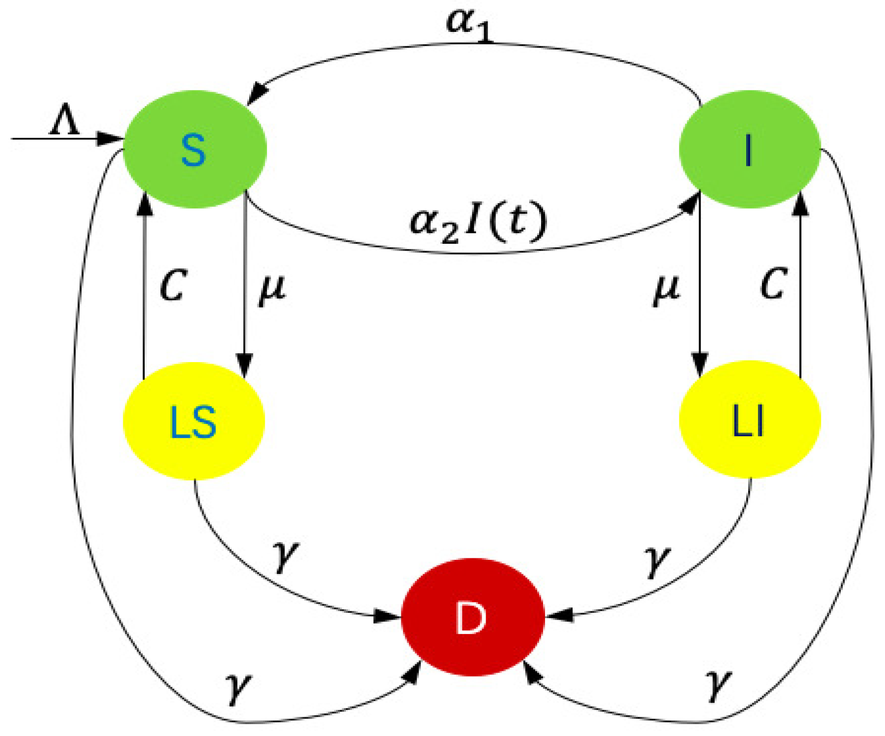
The model presented in this manuscript is global and deterministic such that sensor nodes are classified into five compartments: Susceptible (S), Infected (I), Susceptible in Low-energy (), Infected in Low-energy (), and Dysfunctional (D), as shown in Figure 1. Sensor nodes in S are vulnerable to malware; sensor nodes in I are compromised with malware and perform malicious action; sensor nodes in and state are both in dormant-like state; and, the sensor nodes in D state are completely incapacitated, owing to irreparable hardware damage. Specifically, the dormant-like state indicates the sensor nodes are forced to stop some running modules due to the low remaining energy, including data transmission. Thus, sensor nodes in state do not have the risk of spreading malware.
Sensor nodes in S transform to I once the attached malware starts running. New infectious sensor nodes are generated with and represents the transmission coefficient. In addition to the new sensor nodes, which are governed by , some of the sensor nodes in I are repaired and converted to S at rate . Owing to electricity consumption, sensor nodes in both S and I drop to low-energy at rate . Meanwhile, when considering rechargeable battery equipped in sensor nodes and charging sensor nodes by multiple wireless charging vehicles [41], low-energy sensor nodes rise back to their previous states, since their batteries are full of electricity again. Detailedly, in order to simplify the model, assuming that the charging rate C is a constant. The model is simplified by assuming the same mortality in each compartment. In the Abbreviation Section, a brief description of the parameters is shown.
Moreover, and constrained by:
As t tends to infinity, considering , the feasible region obtained is
Considering the following equations:
and
2.2. Computation of the Steady States and the Basic Reproductive Number
Considering the limit system, we obtain:
and
where .
- The disease-free steady states , where
- The endemic steady state , whereand
Furthermore, the basic reproductive number can be obtained by the next generation matrix method [44].
Set
and
Thus
3. Dynamic Analysis
In this section, the local and global stabilities of both the disease-free point and the epidemic equilibrium point were fully proved. Moreover, an attack-defense game was built to analyze the confrontation between malware and WRSNs.
3.1. Local Stability Analysis
Theorem 1.
The disease-free equilibrium point, , is locally asymptotically stable if .
Proof.
The eigenvalues of the following matrix
are
and
where and . The real parts of the two eigenvalues are both negative if . Besides,
Thus is locally asymptotically stable [45]. On the contrary, is unstable if . □
Theorem 2.
The epidemic equilibrium point, , is locally asymptotically stable if .
Proof.
First of all, the truth exists if and only if is simple to prove.
Subsequently, the characteristic polynomial of the Jacobian matrix of the state functions (1)–(4) in , when is
where
and
Moreover, a simple calculus shows . Thus, if , applying the Routh criterion [46], the local asymptotically stability of follows. □
3.2. Global Stability Analysis
Theorem 3.
The disease-free equilibrium point, , is globally asymptotically stable if .
Proof.
In this proof, the method of Lyapunov function is considered. In general, in the Lyapunov stability analysis [47], the Lyapunov function needs to be positive definite, except for the stable point, and its first derivative needs to be negative definite.
When considering the Lyapunov function , we obtain:
In addition, if and only if and . Moreover, (S, I, ) tends to when t tends to infinity, and the maximum invariant set in is . Thus, Theorem 3 has been proved, after considering the La-Salle Invariance Principle [48]. □
Theorem 4.
The epidemic equilibrium point, , is globally asymptotically stable if .
Proof.
First of all, by referencing [49], the system is uniformly persistent. According to [50], there exists an absorbent compact. Besides, according to Theorem 2, is the unique equilibrium point if .
The second additive compound matrix of Jacobian matrix is given, as follows:
where
and
Set as the directional derivative of the diagonal matrix , then:
Set the matrix
Set
and
Supposing that is a vector in , then the norm of vector that is defined in is
Note that the Lozinskii measure of B is given by the following expression:
where ,
Supposing that , then . Thus, .
Subsequently,
Consequently, applying the theorem in [52], the statement is proved. □
3.3. Optimal Control Strategies
According to differential game theory [53], let us impose a set of hypotheses as follows.
- (a)
- The game in this paper consists of two parties, i.e., malware and WRSN.
- (b)
- (c)
- Define as a set of state variables.
- (d)
- The attacker (i.e., malware) aims at maximizing and the defender (i.e., WRSNs) aims at minimizing , andwhere indicates the cost incurred by I nodes at time t, indicates the terminal cost of corresponding state, and indicates the number of corresponding state at the terminal moment.
Theorem 5.
Proof.
The saddle point in the game exists and it is unique [53]. Subsequently, referencing [54], the game has a value V, such that
In view of (1)–(5) and (55), the Hamiltonian function is constructed as:
where is a set of co-state variables.
By applying the Pontryagin Maximum Principle [55], the constraints of the co-state variables are formulated, as follows.
Besides, the terminal constraints of the co-state variables are formulated as:
where .
Consequently, the optimal strategies are obtained by
□
As a consequence, in the optimal case, when , the malware exerts maximum effort to infect vulnerable sensor nodes; otherwise, it does not propagate. When , the malware exerts the minimum effort to influence the charging process to nodes; otherwise, the nodes accept the charging requests. Moreover, when , WRSNs exert the maximum effort to clear the malware; otherwise, the networks does nothing in removing malware. When , WRSNs exert the maximum effort to charge the nodes; otherwise, nodes do not charge.
4. Simulation
Theorem 1 to Theorem 5 have been further verified here. In Section 4.1, the stable solutions of the system (1)–(5) are obtained and proved, while the impact of charging is analyzed by observing the variation of I nodes. In Section 4.2, the optimal solutions are displayed by comparing with the groups without optimal controls. All of the simulations are based on MacOS Catalina (Intel Core i5, 8 GB, 1.8 GHz) and MATLAB 2017b.
4.1. Stability Analysis
This part aims to test Theorem 1 to Theorem 4. Firstly, eight two-dimensional feasible regions are constructed through the combinations of various state variables to analyze their relationships. Subsequently, suppose that , , , , , and . Therefore, whether or , the total number of sensor nodes is constant at 20 (i.e., ), including the initial value (i.e., ).
4.1.1. Disease-Free Equilibrium Stability
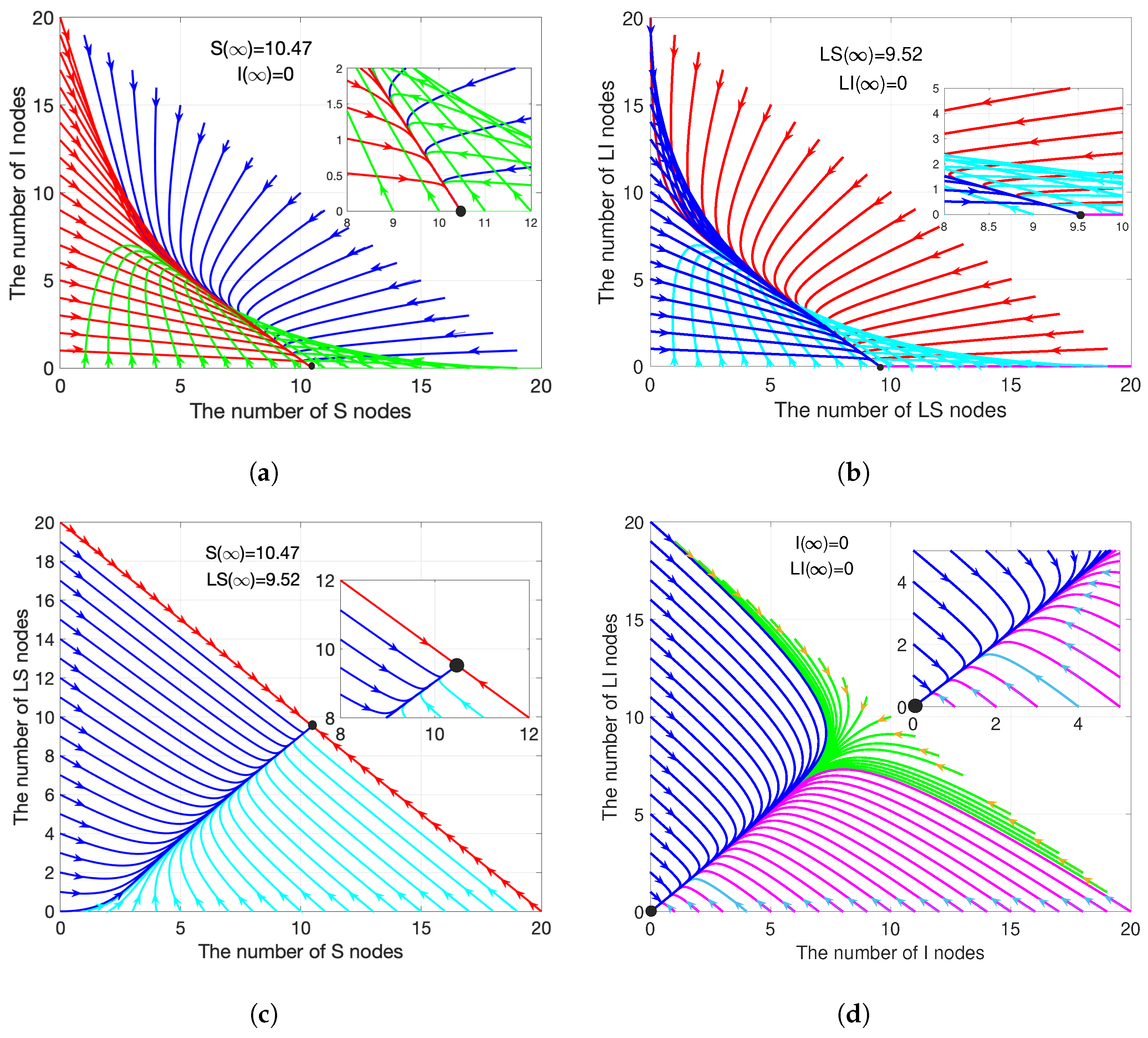
Here, four different state combinations (i.e., , and ) are given in order to testify the disease-free equilibrium point, as shown in Figure 2. At this moment, . Theoretically, , , and , according to (18). Practically, the simulation results that are shown in Figure 2 conform to Theorems 1 and 3.
The evolution in and are similar and so do and , as depicted in Figure 2. In Figure 2a,b, the curve starts from the boundary and finally converges to (10.47, 0)((9.52, 0)). Specifically, as illustrated in Figure 2a,b, the curve in the feasible region is attracted by (). When malware only exists on nodes, a peak in the number of I nodes appears after a period of time. The peak decreases as the initial number of S nodes increases, and it eventually stays around at 3. At the same time, the number of I nodes always shows a downward trend, and it is cleared when . In Figure 2c,d, the curve is attracted by (), and finally converges to (10.47, 9.52)(0, 0). From the beginning, an increase in the number of S() or I() nodes must lead to a decrease in the number of (S) or (I) nodes, as shown in Figure 2c,d. Subsequently, the number of S and nodes increase simultaneously, while the number of I and decrease simultaneously. Consequently, in WRSNs, only S and nodes exist.
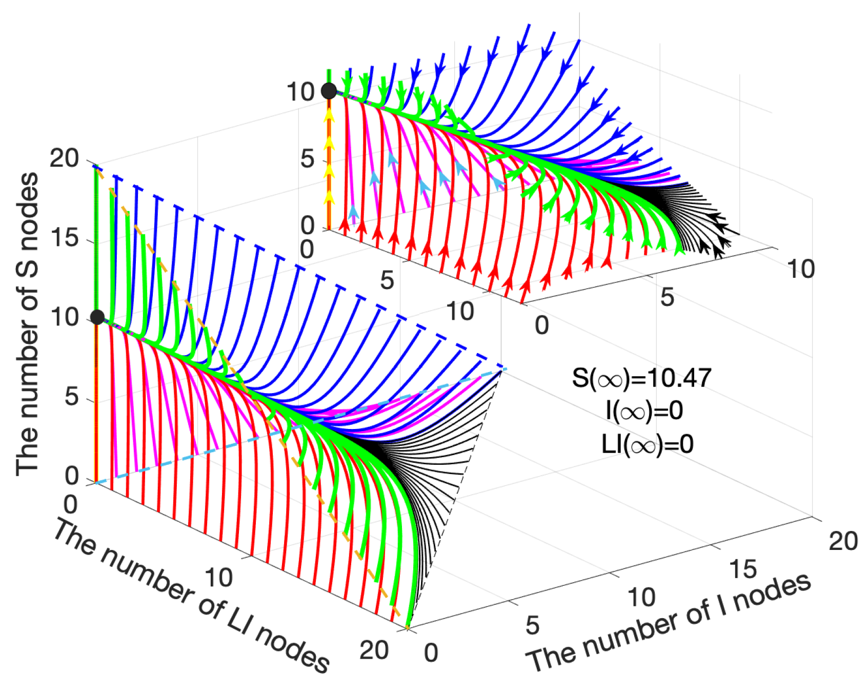
Figure 3 illustrates a three-dimensional diagram of the system(15)–(17), where the feasible region is in the triangular pyramid area. Note that Figure 2a,d are two feasible region planes in Figure 3. Similarly, the curve gathers together, and then finally converges to (10.47, 0, 0). In summary, a smooth transitional period exists before the system reaches equilibrium. During the period, malware is eliminated from the network gradually and the numbers of S and nodes maintain a steady growth. In the end, the malware is totally cleared in the WRSNs, and the numbers of S and nodes remain unchanged under constant charging power.
4.1.2. Epidemic Equilibrium Stability
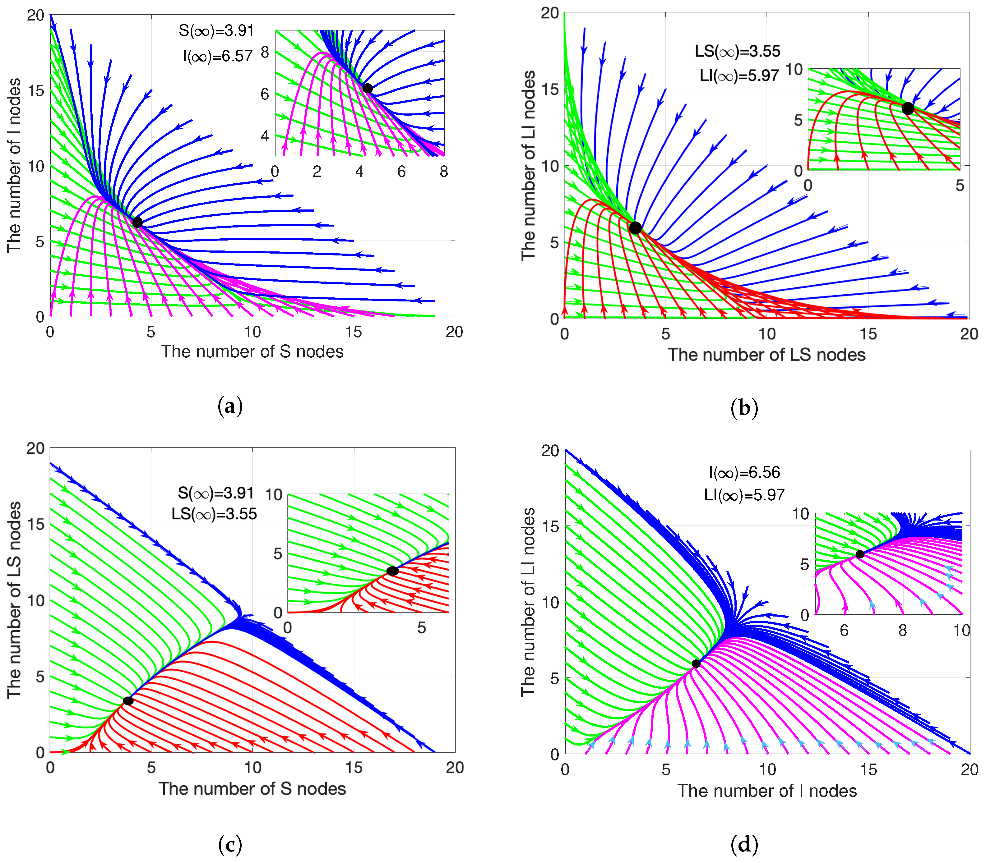
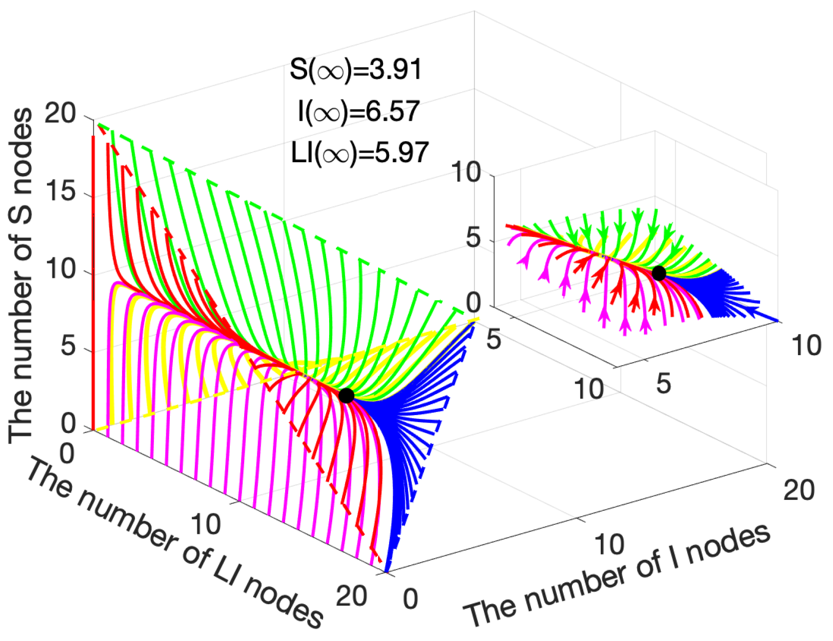
Similarly, the same four combinations are applied here, as depicted in Figure 4. Suppose that the values of coefficients, except for , remain constant, as stated in Section 4.1.1. At this time, . Substitute the coefficients into (19)–(21), we obtained , and . Moreover, the results that are presented in Figure 5 confirm Theorem 2 and Theorem 4.
When compared with Figure 2, when , the equilibrium points appear inside the region, but not the boundary. In terms of evolution trends, Figure 4a,c and Figure 4b,d are close. It is worth noting that the prerequisite for the existence of the epidemic equilibrium point is that at least one I node exists. When compared with the case , at this time, the number of I() nodes is no longer reduced. The curve that is shown in Figure 4a,b eventually converges to (3.91, 6.57) (3.55, 5.97). In particular, when the initial number of I() nodes is less than 6.57(5.97), the number of I() nodes will increase significantly after a gentle decline, as shown in Figure 4a,b. The curve that is presented in Figure 4a,b is attracted by (), and it finally converges to the equilibrium point along it.
When compared with the case , the evolution curves of are similar at first. However, when the curves gather, they do not just show a single evolution trend, but the increase and decrease appear at the same time, as shown in Figure 4c,d. In Figure 4c,d, the curve begins from the boundary and it converges to (3.91, 3.55) (6.56, 5.97), when .
Figure 5 illustrates the limit system (15)–(17) in three-dimensional way. Similarly, Figure 4a,d are the planes into the triangular pyramid region. Similar to the case , the evolution of S, I, and nodes has a smooth transitional period before reaching the equilibrium point. During the transitional period, when the number of , the trend drops to (3.91, 6.57, 5.97); when the number of , the trend rises to (3.91, 6.57, 5.97). In summary, in the case , if malware propagates on a large scale in WRSNs, after a period of time, the numbers of I and nodes will decrease along a specific trajectory. Meanwhile, the numbers of S and nodes increase along a specific trajectory, and finally converge to (3.91, 6.57, 5.97). Conversely, when few malware exists in WRSNs, over a period of evolution, the numbers of S and nodes decrease along the specific trajectory, and the numbers of I and increase along the specific trajectory, and finally converge to (3.91, 6.57, 5.97).
4.1.3. Influence of the Charging Rate C
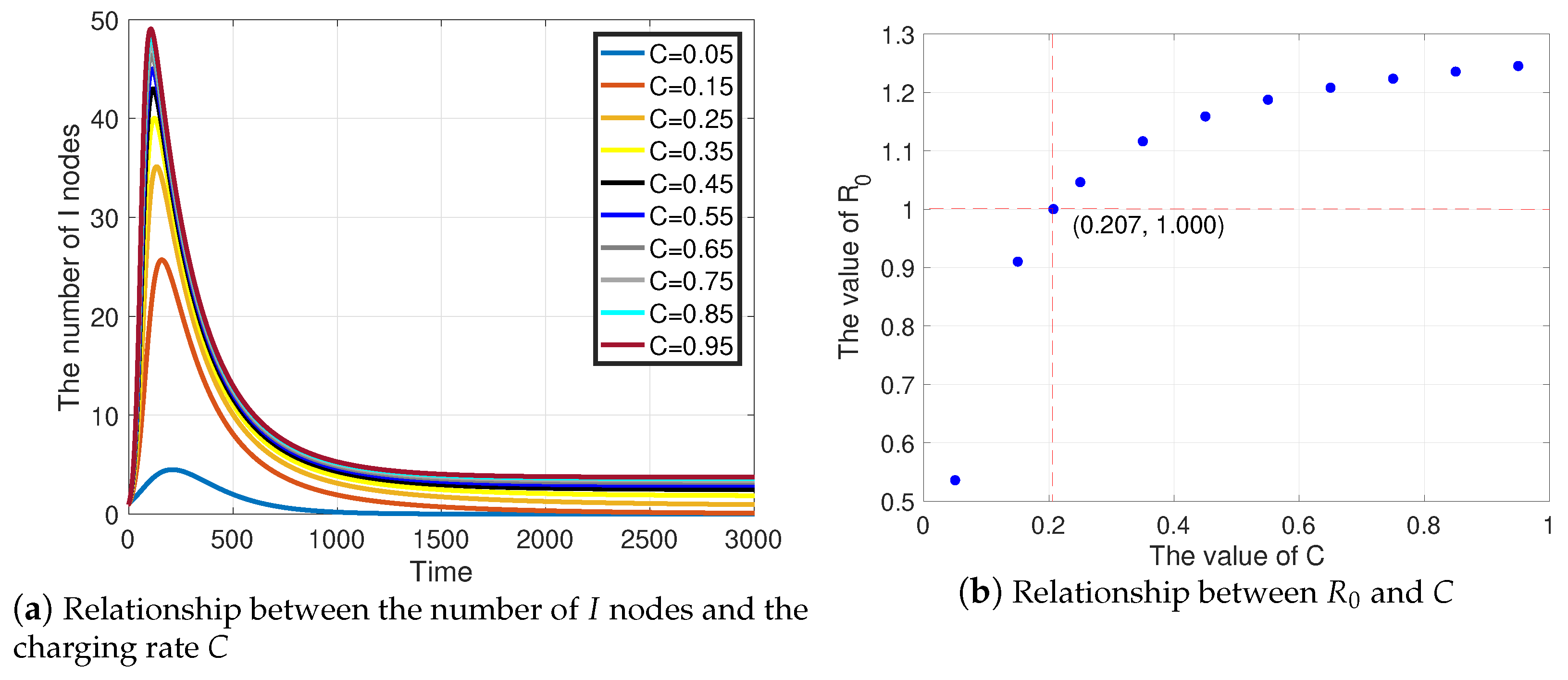
The influence of charging rate is discussed detailedly by comparing the quantity of I nodes with various C, as shown in Figure 6. Based on (55), C directly affects , thereby affecting the prevalence of malware. As C increases, the peak of the quantity of I nodes keeps growing and gradually saturates, as shown in Figure 6a. Under ten sets of C, only and clear the malware. After simple calculation, we find, as C increases, that grows likewise, as illustrated in Figure 6b. Specifically, , when , which indicates, when , that the malware is eliminated if and prevalent if .
Such results reveal that, in WRSNs, in the confrontation with malware, the higher charging power, the higher peak of malware propagation. This inspires us to properly control the charging rate in order to prevent the prevalence of malware.
4.2. Optimal Control
In this section, we further classify Theorem 5 into three aspects: evolution of state variables, overall cost and variation of control variables. The coefficients remain constant as set in Section 4.1. Moreover, set , , , , , , , , and . In particular, this section analyzes the two cases of (i.e., and ). Furthermore, the optimality of the strategies (57)–(60) is highlighted by comparison with the non-optimal control groups.
Evolution of State Variables
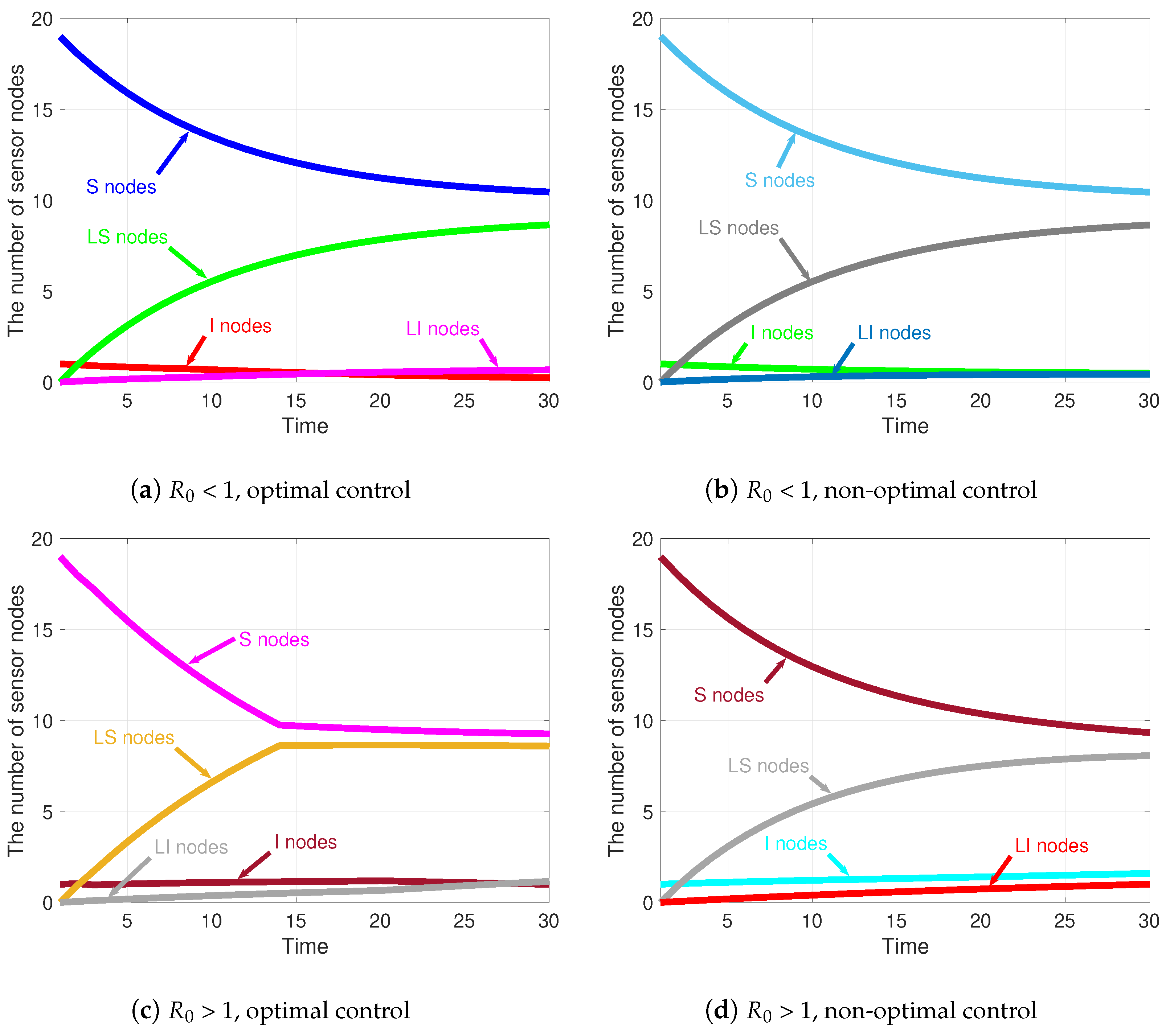
In this part, the evolution of state variables under four cases is discussed, as shown in Figure 7.
The evolution trends of S and nodes are very close in the four cases. Specifically, when , in Case 1, and ; in Case 2, and ; in Case 3, and ; and, in Case 4, and . When (i.e., Case 1 and Case 2), the number of I nodes always keeps decreasing. However, when (i.e., Case 3 and Case 4), the number of nodes shows increasing signs. As for nodes, the number keeps rising in all four cases. Detailedly, when , in Case 1, and ; in Case 2, and ; in Case 3, and ; and, in Case 4, and .
The results indicate, in the consecutive attack-defense confrontation game, that the number of I nodes decays faster than that of the control groups. Therefore, the Susceptible, Infected, Low-energy, Susceptible (SILS) model under dynamic optimal controls is more conducive to the clearance of malware in WRSNs.
4.3. Overall Cost and Optimal Controls
In this part, the four cases stated above are explained further in two aspects, including accumulative costs and variation on control variables.
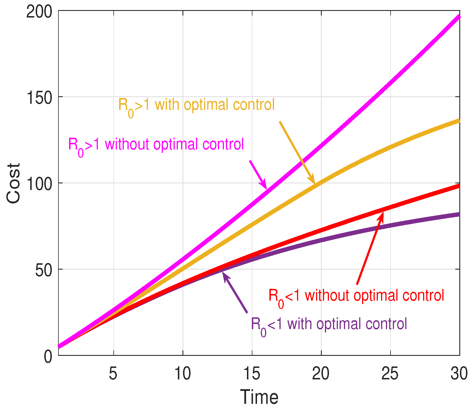
Figure 8 illustrates the cost under the four cases. From Figure 8, it can be seen that the cost with optimal control is lower than that of the control group all of the time, which indicates the validity. Specifically, in Case 1, the cost finally reaches 81.9044; in Case 2, the cost finally reaches 98.4576; in Case 3, the cost finally reaches 162.8256; and, in Case 4, the cost finally reaches 196.9237. The cost depends on the number of I nodes based on (55). Thus, the cumulative cost is another embodiment of variation on the number of I nodes. It can be seen, even under optimal control, that the number of I nodes when is still greater than that when .
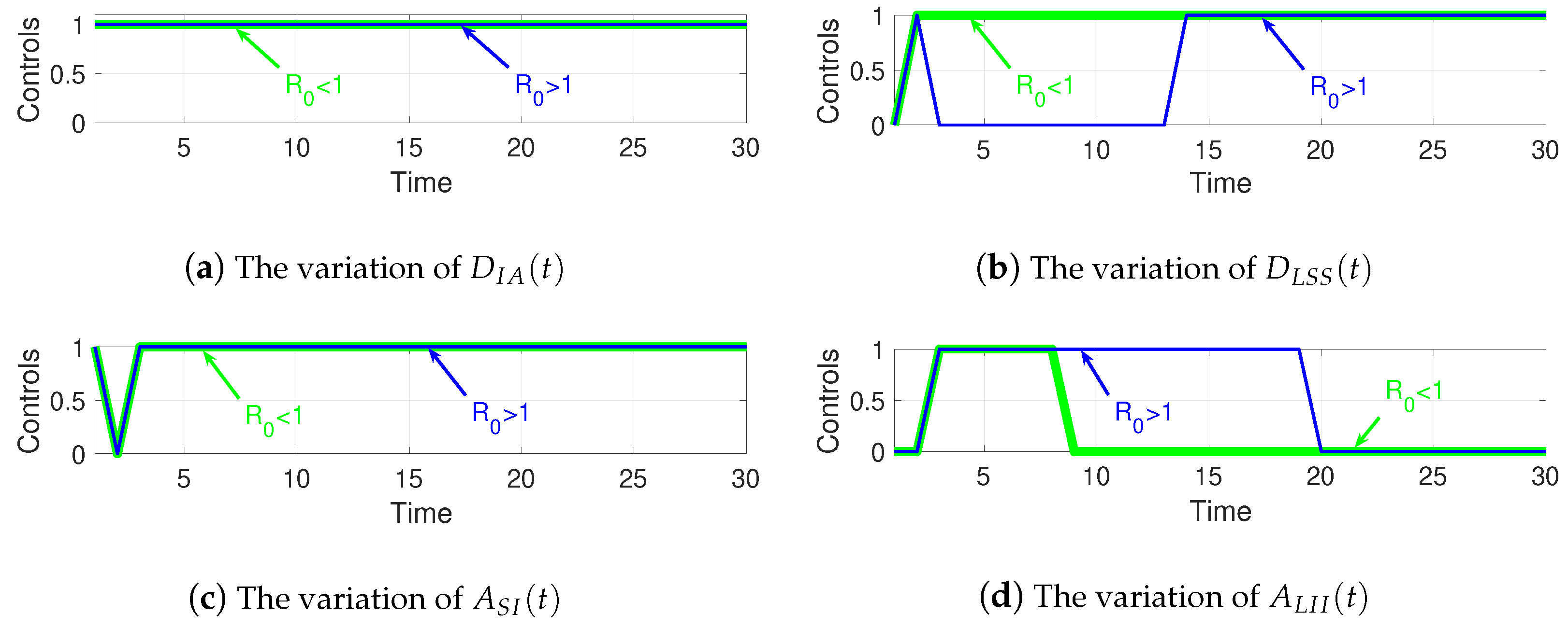
Figure 9 depicts the variations of the control variables when and obtained from (57)–(60). Among them, Figure 9a shows the variation of , Figure 9b shows the variation of , Figure 9c shows the variation of , and Figure 9d shows the variation of .
For WRSNs, its purpose is to minimize the cost. Therefore, whether or , WRSNs are sparing no effort to remove malware, as depicted in Figure 9a. However, the charging process is not always performed. After charging started, in the case of , owing to the excessive growth of malware, the charging of nodes stops immediately, as shown in Figure 9b.
Regarding malware, its aim is to maximize the cost. Thus, in both cases, malware is being copied and propagated almost all of the time, as depicted in Figure 9c. Similarly, nodes do not always receive charging requests. If the sharp decline in the number of I nodes appears (i.e., when and when ), charging nodes will cause more malware to be removed, which is unconducive to the spread of the malware.
5. Conclusions
A novel model, namely SILS, has been proposed when considering the remaining energy of WRSNs in this paper. In SILS, sensor nodes are divided into five states: susceptible, infected, susceptible in low-energy, infected in low-energy, and dysfunctional. After theoretically proposing local and global stability, we further verify them by simulations. The simulation results indicate some characteristics of the SILS model: before reaching the equilibrium point ( or ), there exists a phenomenon that the number of S(I) and () nodes increases or decreases linearly simultaneously. Besides, the positive relationship between charging rate C and basic reproductive number is revealed, which enlightens us to adjust the charging rate C reasonably. Meanwhile, the threshold of C is obtained, which is, if C is higher than the threshold, malware will be prevalent, and below the threshold, malware will be eliminated. In addition to analyzing the stability, by constructing a game model, we further analyze the attack-defense methods of malware and WRSNs, and derive the optimal strategies for both players. At the same time, by comparing the cases and , the simulation results show that the optimal controls can effectively inhibit the growth of I nodes and reduce the overall costs.
This paper discusses a static, homogeneous network. However, with the continuous development of the Internet of Things industry and the integration of various terminal devices, heterogeneous network technology has become mainstream and it is one of our future research areas. At the same time, the convenience that is brought by the mobile technology has became increasingly prominent, such as mobile base stations and mobile chargers. However, the potential safety hazards that are caused by the mobile devices cannot be ignored. Moreover, with the investigation of the actual situation and the deepening of the mathematical model, various random model problems will be raised, which are also the trends in our future research.
Author Contributions
Conceptualization, G.L. and B.P.; methodology, G.L., B.P. and X.Z.; software, B.P.; validation, G.L., B.P. and X.Z.; formal analysis, B.P.; investigation, G.L. and B.P.; writing–original draft preparation, B.P.; writing–review and editing, G.L., B.P. and X.Z.; project administration, G.L.; funding acquisition, G.L. All authors have read and agreed to the published version of the manuscript.
Funding
This work was partially supported by the National Natural Science Foundation of China (No. 61403089).
Data Availability Statement
The data presented in this study are available on request from the corresponding author. The data are no publicly available as they involve the subsequent application of patent for invention and the publication of project deliverables.
Conflicts of Interest
The authors declare that they have no known competing financial interests or personal relationships that could have appeared to influence the work reported in this paper.
Abbreviations
The following abbreviations are used in this manuscript:
| Symbol | Description |
| Birth rate | |
| Death rate | |
| Depletion rate | |
| Removal rate | |
| C | Charging rate |
| Transmission rate |
References
- Rashid, B.; Rehmani, M.H. Applications of wireless sensor networks for urban areas: A survey. J. Netw. Comput. Appl. 2016, 60. [Google Scholar] [CrossRef]
- Yetgin, H.; Cheung, K.T.K.; El-Hajjar, M.; Hanzo, L. A Survey of Network Lifetime Maximization Techniques in Wireless Sensor Networks. IEEE Commun. Surv. Tutor. 2017, 19, 828–854. [Google Scholar] [CrossRef] [Green Version]
- Zhang, F.; Zhang, J.; Qian, Y.J. A Survey on Wireless Power Transfer based Charging Scheduling Schemes in Wireless Rechargeable Sensor Networks. In Proceedings of the ICCSSE 2018, Wuhan, China, 21–23 August 2018. [Google Scholar]
- Shu, Y.C.; Yousefi, H.; Cheng, P.; Chen, J.M.; Gu, Y.; He, T.; Shin, K.G. Near-Optimal Velocity Control for Mobile Charging in Wireless Rechargeable Sensor Networks. IEEE. Trans. Mob. Comput. 2016, 15, 1699–1713. [Google Scholar] [CrossRef] [Green Version]
- Wu, P.F.; Xiao, F.; Sha, C.; Huang, H.P.; Sun, L.J. Trajectory Optimization for UAVs’ Efficient Charging in Wireless Rechargeable Sensor Networks. IEEE Trans. Veh. Technol. 2020, 69, 4207–4220. [Google Scholar] [CrossRef]
- Mo, L.; Kritikakou, A.; He, S.B. Energy-Aware Multiple Mobile Chargers Coordination for Wireless Rechargeable Sensor Networks. IEEE Internet Things J. 2019, 6, 8202–8214. [Google Scholar] [CrossRef] [Green Version]
- Lin, C.; Shang, Z.; Du, W.; Ren, J.K.; Wang, L.; Wu, G.W. CoDoC: A Novel Attack for Wireless Rechargeable Sensor Networks through Denial of Charge. In Proceedings of the IEEE INFOCOM 2019, Paris, France, 29 April–2 May 2019. [Google Scholar]
- Lin, C.; Zhou, J.Z.; Guo, C.Y.; Song, H.B.; Wu, G.W.; Mohammad, S.O. TSCA: A temporal-spatial real-time charging scheduling algorithm for on-demand architecture in wireless rechargeable sensor networks. IEEE. Trans. Mob. Comput. 2018, 17, 211–224. [Google Scholar] [CrossRef]
- Han, G.J.; Miao, X.; Wang, H.; Guizani, M.; Zhang, W.B. CPSLP: A Cloud-Based Scheme for Protecting Source Location Privacy in Wireless Sensor Networks Using Multi-Sinks. IEEE Trans. Veh. Technol. 2019, 68, 2739–2750. [Google Scholar] [CrossRef]
- EI Shafie, A.; Niyato, D.; AI-Dhahir, N. Security of Rechargeable Energy-Harvesting Transmitters in Wireless Networks. IEEE Wirel. Commun. Lett. 2016, 5, 384–387. [Google Scholar] [CrossRef] [Green Version]
- Bhushan, B.; Sahoo, G. E2SR2: An acknowledgement-based mobile sink routing protocol with rechargeable sensors for wireless sensor networks. Wirel. Netw 2019, 25, 2697–2721. [Google Scholar] [CrossRef]
- Saidi, A.; Benahmed, K.; Seddiki, N. Secure cluster head election algorithm and misbehavior detection approach based on trust management technique for clustered wireless sensor networks. Ad Hoc Netw. 2020, 106, 102215. [Google Scholar] [CrossRef]
- Wang, G.; Lee, B.; Ahn, J.; Cho, G. A UAV-assisted CH election framework for secure data collection in wireless sensor networks. Futur. Gener. Comp. Syst. 2020, 102, 152–162. [Google Scholar] [CrossRef]
- Karyotis, V.; Khouzani, M.H.R. Malware Diffusion Models for Modern Complex Networks: Theory and Applications; Morgan Kaufmann: Burlington, MA, USA, 2016. [Google Scholar]
- Cui, B.J.; Jin, H.F.; Carullo, G.; Liu, Z.L. Service-oriented mobile malware detection system based on mining strategies. Pervasive Mob. Comput. 2015, 2015, 101–116. [Google Scholar] [CrossRef]
- Jaint, B.; Indu, S.; Pandey, N.; Pahwa, K. Malicious Node Detection in Wireless Sensor Networks Using Support Vector Machine. In Proceedings of the International Conference on Recent Developments in Control, Automation & Power Engineering, Noida, India, 10–11 October 2019; pp. 247–252. [Google Scholar]
- Thaile, M.; Ramanaiah, O.B.V. Node Compromise Detection Based on NodeTrust in Wireless Sensor Networks. In Proceedings of the International Conference on Computer Communication and Informatics, Coimbatore, India, 7–9 January 2016. [Google Scholar]
- Butun, I.; Osterberg, P.; Song, H.B. Security of the Internet of Things: Vulnerabilities, Attacks, and Countermeasures. IEEE Commun. Sur. Tutor. 2020, 22, 616–644. [Google Scholar] [CrossRef] [Green Version]
- Ai, J.J.; Chen, H.C.; Guo, Z.H.; Cheng, G.Z.; Baker, T. Mitigating malicious packets attack via vulnerability-aware heterogeneous network devices assignment. Futur. Gener. Comp. Syst. 2020, 111, 841–852. [Google Scholar] [CrossRef]
- Hernández Guillén, J.D.; Martín del Rey, A. A mathematical model for malware spread on WSNs with population dynamics. Phys. A 2020, 545, 123609. [Google Scholar]
- Huang, D.W.; Yang, L.X.; Yang, X.F.; Wu, Y.B.; Tang, Y.Y. Towards understanding the effectiveness of patch injection. Phys. A 2019, 526, 120956. [Google Scholar] [CrossRef]
- Zhu, L.H.; Zhou, M.T.; Zhang, Z.D. Dynamical Analysis and Control Strategies of Rumor Spreading Models in Both Homogeneous and Heterogeneous Networks. J. Nonlinear Sci. 2020, 30, 2545–2576. [Google Scholar] [CrossRef]
- Shen, S.G.; Zhou, H.P.; Feng, S.; Liu, J.H.; Zhang, H.; Cao, Q.Y. An Epidemiology-Based Model for Disclosing Dynamics of Malware Propagation in Heterogeneous and Mobile WSNs. IEEE Access 2020, 8, 43876–43887. [Google Scholar] [CrossRef]
- Zhu, L.H.; Guan, G. Dynamical analysis of a rumor spreading model with self-discrimination and time delay in complex networks. Phys. A 2019, 533, 121953. [Google Scholar] [CrossRef]
- Srivastava, P.K.; Pandey, S.P.; Gupta, N.; Singh, S.P.; Ojha, R.P. Modeling and Analysis of Antimalware Effect on Wireless Sensor Network. In Proceedings of the ICCCS 2019, Singapore, 23–25 February 2019. [Google Scholar]
- Hosseini, S.; Azgomi, M.A. The dynamics of an SEIRS-QV malware propagation model in heterogeneous networks. Phys. A 2018, 512, 803–817. [Google Scholar] [CrossRef]
- Ojha, R.P.; Srivastava, P.K.; Sanyal, G.; Gupta, N. Improved Model for the Stability Analysis of Wireless Sensor Network Against Malware Attacks. Wirel. Pers. Commun. 2020. [Google Scholar] [CrossRef]
- Biswal, S.R.; Swain, S.K. Model for Study of Malware Propagation Dynamics in Wireless Sensor Network. In Proceedings of the ICOEI 2019, Tirunelveli, India, 23–25 April 2019. [Google Scholar]
- Al-Tous, H.; Barhumi, I. Differential Game for Resource Allocation in Energy Harvesting Sensor Networks. In Proceedings of the IEEE ICC 2018, Kansas City, MO, USA, 20–24 May 2018. [Google Scholar]
- Huang, Y.H.; Zhu, Q.Y. A Differential Game Approach to Decentralized Virus-Resistant Weight Adaptation Policy Over Complex Networks. IEEE Trans. Control Netw. Syst. 2020, 7, 944–955. [Google Scholar] [CrossRef] [Green Version]
- Zhang, L.T.; Xu, J. Differential Security Game in Heterogeneous Device-to-Device Offloading Network Under Epidemic Risks. IEEE Trans. Netw. Sci. Eng. 2020, 7, 1852–1861. [Google Scholar] [CrossRef]
- Shen, S.G.; Li, H.J.; Han, R.S.; Vasilakos, A.V.; Wang, Y.H.; Cao, Q.Y. Differential Game-Based Strategies for Preventing Malware Propagation in Wireless Sensor Networks. IEEE Trans. Inf. Forensics Secur. 2014, 9, 1962–1973. [Google Scholar] [CrossRef]
- Liu, G.Y.; Peng, B.H.; Zhong, X.J.; Cheng, L.F.; Li, Z.F. Attack-Defense Game between Malicious Programs and Energy-Harvesting Wireless Sensor Networks Based on Epidemic Modeling. Complexity 2020, 2020, 3680518. [Google Scholar] [CrossRef]
- Miao, L.; Li, S. A Differential Game-Theoretic Approach for the Intrusion Prevention Systems and Attackers in Wireless Networks. Wirel. Pers. Commun. 2018, 103, 1993–2003. [Google Scholar] [CrossRef]
- Zhang, H.W.; Jiang, L.; Huang, S.R.; Wang, J.D.; Zhang, Y.C. Attack-Defense Differential Game Model for Network Defense Strategy Selection. IEEE Access 2019, 7, 50618–50629. [Google Scholar] [CrossRef]
- Hu, J.H.; Qian, Q.; Fang, A.; Fang, S.Z.; Xie, Y. Optimal Data Transmission Strategy for Healthcare- Based Wireless Sensor Networks: A Stochastic Differential Game Approach. Wirel. Pers. Commun. 2016, 89, 1295–1313. [Google Scholar] [CrossRef]
- Sun, Y.; Li, Y.B.; Chen, X.H.; Li, J. Optimal defense strategy model based on differential game in edge computing. J. Intell. Fuzzy Syst. 2020, 39, 1449–1459. [Google Scholar] [CrossRef]
- Eshghi, S.; Khouzani, M.H.R.; Sarkar, S. Optimal Patching in Clustered Malware Epidemics. IEEE-ACM Trans. Netw. 2016, 24, 283–298. [Google Scholar] [CrossRef] [Green Version]
- Khouzani, M.H.R.; Sarkar, S.; Altman, E. Optimal Dissemination of Security Patches in Mobile Wireless Networks. IEEE Trans. Inf. Theory 2012, 58, 4714–4732. [Google Scholar] [CrossRef]
- Sarkar, S.; Khouzani, M.H.R.; Kar, K. Optimal Routing and Scheduling in Multihop Wireless Renewable Energy Networks. IEEE Trans. Autom. Control 2013, 58. [Google Scholar] [CrossRef] [Green Version]
- Wang, K.; Wang, L.; Lin, C.; Obaidat, M.S.; Alam, M. Prolonging lifetime for wireless rechargeable sensor networks through sleeping and charging scheduling. Int. J. Commun. Syst. 2020, 33, e4355. [Google Scholar] [CrossRef]
- Yorke, J.A. Invariance for ordinary differential equations. Math. Syst. Theory 1967, 1, 353–372. [Google Scholar] [CrossRef]
- Wiggins, S. Introduction to Applied Nonlinear Dynamical Systems and Chaos; Springer: New York, NY, USA, 2003; Volume 2. [Google Scholar]
- Diekmann, O.; Heesterbeek, H.; Britton, T. Mathematical Tools for Understanding Infectious Disease Dynamics; Princeton University Press: Princeton, NJ, USA, 2013. [Google Scholar]
- van den Diressche, P.; Watmough, J. Further notes on the basic reproduction number. In Mathematical Epidemiology; Brauer, F., van den Driessche, P., Wu, J., Eds.; Springer: Berlin/Heisenberg, Germany, 2008; pp. 159–178. [Google Scholar]
- Merkin, D.R. Introduction to the Theory of the Stability; Springer: New York, NY, USA, 2012; Volume 24. [Google Scholar]
- Lyapunov, A.M. The general problem of the stability of motion. Int. J. Control 1992, 55, 531–534. [Google Scholar] [CrossRef]
- Lasalle, J.P. The Stability of Dynamical Systems; SIAM: Philadelphia, PA, USA, 1976. [Google Scholar]
- Freedman, H.; Ruan, S.; Tang, M. Uniform persistence and flows near a closed positively invariant set. J. Dyn. Differ. Equ. 1994, 6, 583–600. [Google Scholar] [CrossRef] [Green Version]
- Hutson, V.; Schmitt, K. Permanence and the dynamics of biological systems. Math. Biosci. 1992, 111, 1–71. [Google Scholar] [CrossRef]
- Li, M.L.; Muldowney, J.S. A geometric approach to the global-stability problems. J. Math. Anal. 1996, 27, 1070–1083. [Google Scholar] [CrossRef]
- Cushing, J.M. Nonlinear matrix models and population dynamics. Nat. Resour. Model. 1988, 2, 539–580. [Google Scholar] [CrossRef]
- Avner, F. Differential games. In Handbook of Game Theory; Aumann, R.J., Hart, S., Eds.; Elsevier: Amsterdam, The Netherlands, 1994; Volume 2. [Google Scholar]
- Bressan, A. Noncooperative differential games. Milan J. Math. 2011, 79, 357–427. [Google Scholar] [CrossRef]
- Isaacs, R. Differential Game; Wiley: New York, NY, USA, 1965. [Google Scholar]
Figure 1.
Flow diagram of the Susceptible, Infected, Low-energy, Susceptible (SILS) Model.

Figure 2.
Evolution of sensor nodes when . Different colors indicate that the curves start at different boundaries. So do Figure 3, Figure 4 and Figure 5.

Figure 3.
Variation of S, I and LI nodes when .

Figure 4.
Evolution of sensor nodes when .

Figure 5.
Variation of S, I and LI nodes when .

Figure 6.
The influence of C.

Figure 7.
Evolution of sensor nodes under four different cases.

Figure 8.
Overall cost.

Figure 9.
Variation of control variables.


Table 1.
Researches on stability of epidemic model in Wireless sensor networks (WSNs).
| Authors | Model | Characteristics | Stability |
|---|---|---|---|
| J.D. HernándezGuillén et al. [20] | SCIRS | Considering the carrier state, population dynamics, and vaccination and reinfection processes | Local and global stability in malware-free and epidemic points |
| S.G. Shen et al. [23] | VCQPS | Considering both the heterogeneity and mobility of heterogeneous and mobile sensor nodes | Local and global stability in malware-free point |
| Linhe Zhu et al. [24] | SBD | Considering the nonlinear incidence rate and time delay in complex networks | Local and global stability in rumor-free point |
| P.K. Srivastava et al. [25] | SEIAR | Considering the anti-malware process | Local and global stability in worm-free point |
| S. Hosseini et al. [26] | SEIRS-QV | Considering the impacts of user awareness, network delay and diverse configuration of nodes | Local and global stability in malware-free point |
| D.W. Huang et al. [21] | SIPS | Considering the patch injection mechanism | Local and global stability in epidemic point |
| L.H. Zhu et al. [22] | I2S2R | Considering the effect of time delay both in homogeneous networks and heterogeneous networks | Local and global stability in malware-free and epidemic points |
| R.P. Ojha et al. [27] | SEIQRV | Considering both quarantine and vaccination techniques | Local and global stability in worm-free point |
| S.R. Biswal et al. [28] | SEIRD | Considering the early detection and removal process | Local and global stability in worm-free point |
Table 2.
Researches on differential game applied in WSNs.
| Authors | Participants | Goal |
|---|---|---|
| H. Al-Tous et al. [29] | An energy-harvesting (EH) multi-hop wireless sensor network (WSN) | Adaptively changing the transmitted data and power, efficiently utilizing the available harvested energy and balancing the buffer of all sensor nodes. |
| Y.H. Huang et al. [30] | Virus and nodes with various weights | Minimizing the total cost of the whole network |
| L.T. Zhang, et al. [31] | Device to Device (D2D) offloading enabled mobile network and malware | D2D offloading enabled mobile network aims to maximize the cost |
| S.G. Shen et al. [32] | WSNs and malware | The systems aims to minimize the cost; the malware aims to maximize the cost (the same cost function) |
| G.Y. Liu et al. [33] | WRSNs and malware | WRSNs aims to minimize the cost; malware aims to maximize the cost (the same cost) |
| L. Miao et al. [34] | Intrusion prevention systems(IPS) and the malicious attackers | IPS aims to minimize the cost A; attacker aims to maximize the cost B (two different cost functions ) |
| H.W. Zhang et al. [35] | Attacker and defender | Attacker aims to maximize the cost A; Defender aims to minimize the cost B (two different cost functions) |
| J.H. Hu et al. [36] | Healthcare-based wireless sensor network (HWSN) | HWSN aims to minimizing the transmission cost |
| Y. Sun et al. [37] | Edge nodes (ENs) | ENs aims to minimize the resource consumption |
| S. Eshghi et al. [38] | Mobile WSNs and malware | Mobile WNSs aims to minimize the cost by using optimal patching policies |
| M.H.R. Khouzani et al. [39] | Mobile WSNs and malware | By obtaining the optimal dissemination of patches, the tradeoff between security risks and bandwidth is minimized |
| S. Sarkar et al. [40] | Multi-hop wireless networks | By using the optimal routing and scheduling, the throughput of the networks is optimized |
Publisher’s Note: MDPI stays neutral with regard to jurisdictional claims in published maps and institutional affiliations. |
© 2020 by the authors. Licensee MDPI, Basel, Switzerland. This article is an open access article distributed under the terms and conditions of the Creative Commons Attribution (CC BY) license (http://creativecommons.org/licenses/by/4.0/).
Share and Cite
MDPI and ACS Style
Liu, G.; Peng, B.; Zhong, X. A Novel Epidemic Model for Wireless Rechargeable Sensor Network Security. Sensors 2021, 21, 123. https://doi.org/10.3390/s21010123
AMA Style
Liu G, Peng B, Zhong X. A Novel Epidemic Model for Wireless Rechargeable Sensor Network Security. Sensors. 2021; 21(1):123. https://doi.org/10.3390/s21010123
Chicago/Turabian StyleLiu, Guiyun, Baihao Peng, and Xiaojing Zhong. 2021. "A Novel Epidemic Model for Wireless Rechargeable Sensor Network Security" Sensors 21, no. 1: 123. https://doi.org/10.3390/s21010123
Note that from the first issue of 2016, this journal uses article numbers instead of page numbers. See further details here.