A Simplified Numerical Approach to Examine the Sensitivity of Two-Electrode Capacitance Sensor Orientation to Capture Different Gas–Liquid Flow Patterns in a Small Circular Pipe

 ,
,  , and
, and
Abstract
:
1. Introduction
1.1. Sensors in Multiphase Flow
1.2. Two-Electrode Capacitance Sensors in Gas–Liquid Multiphase Flow
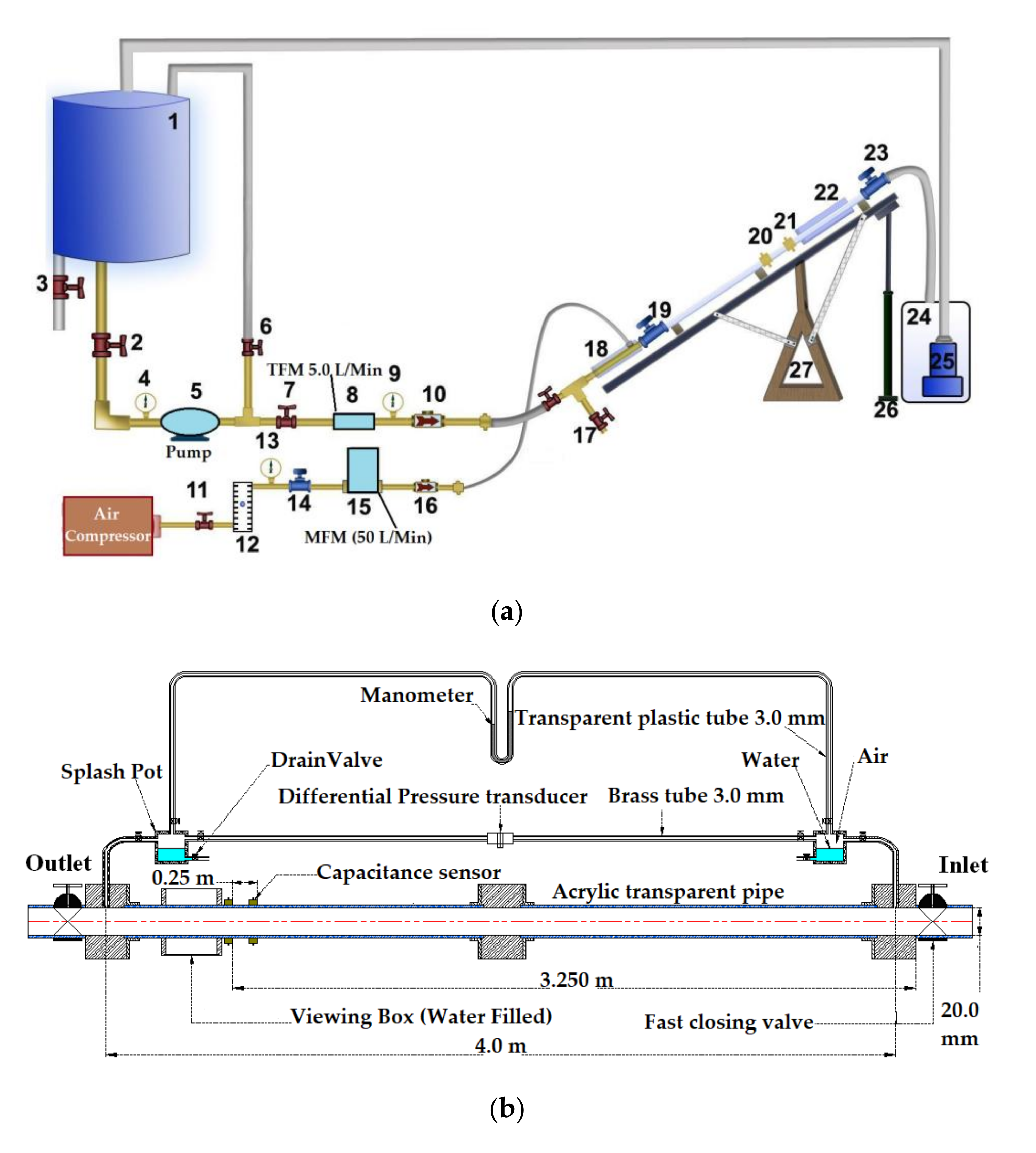
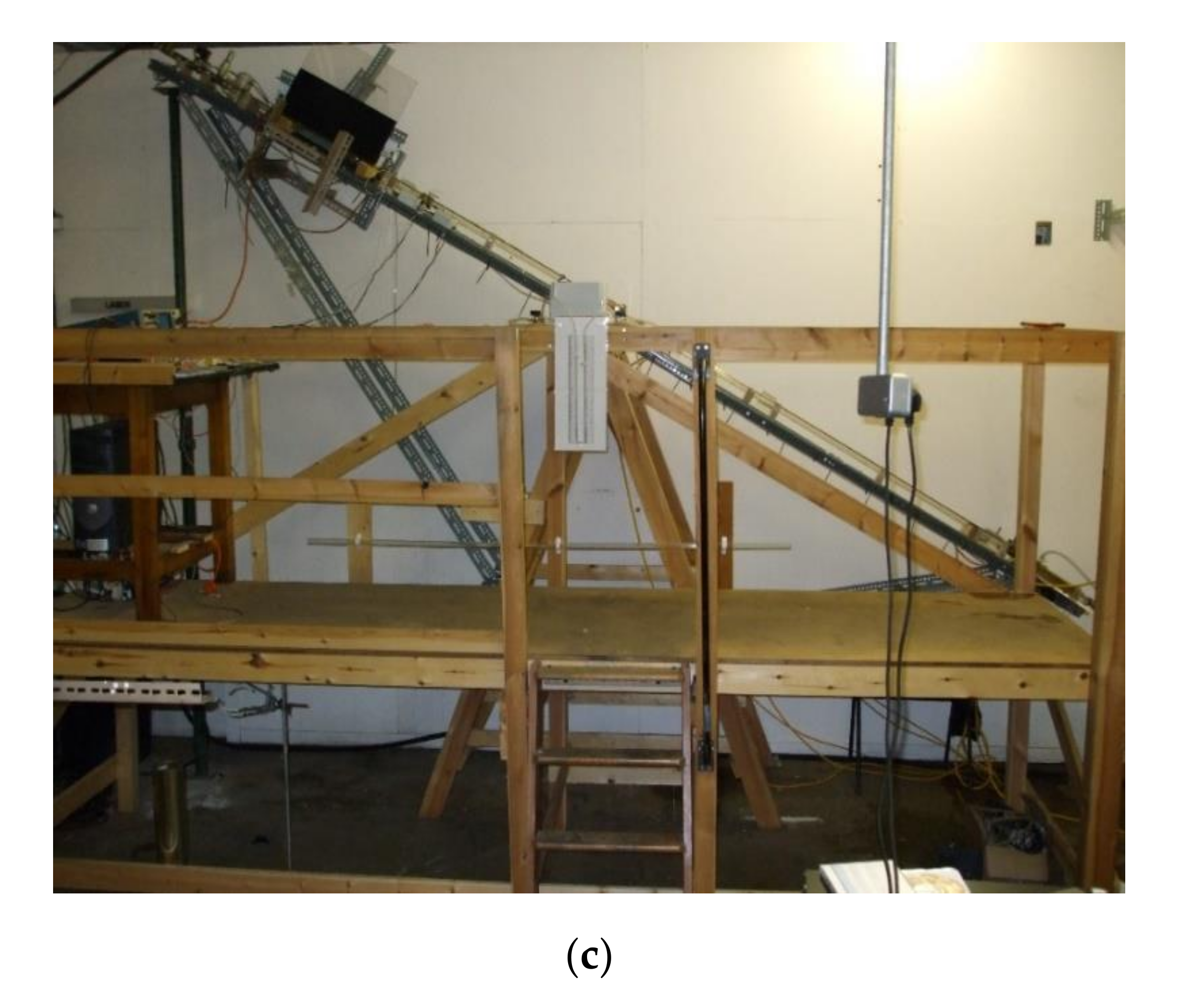
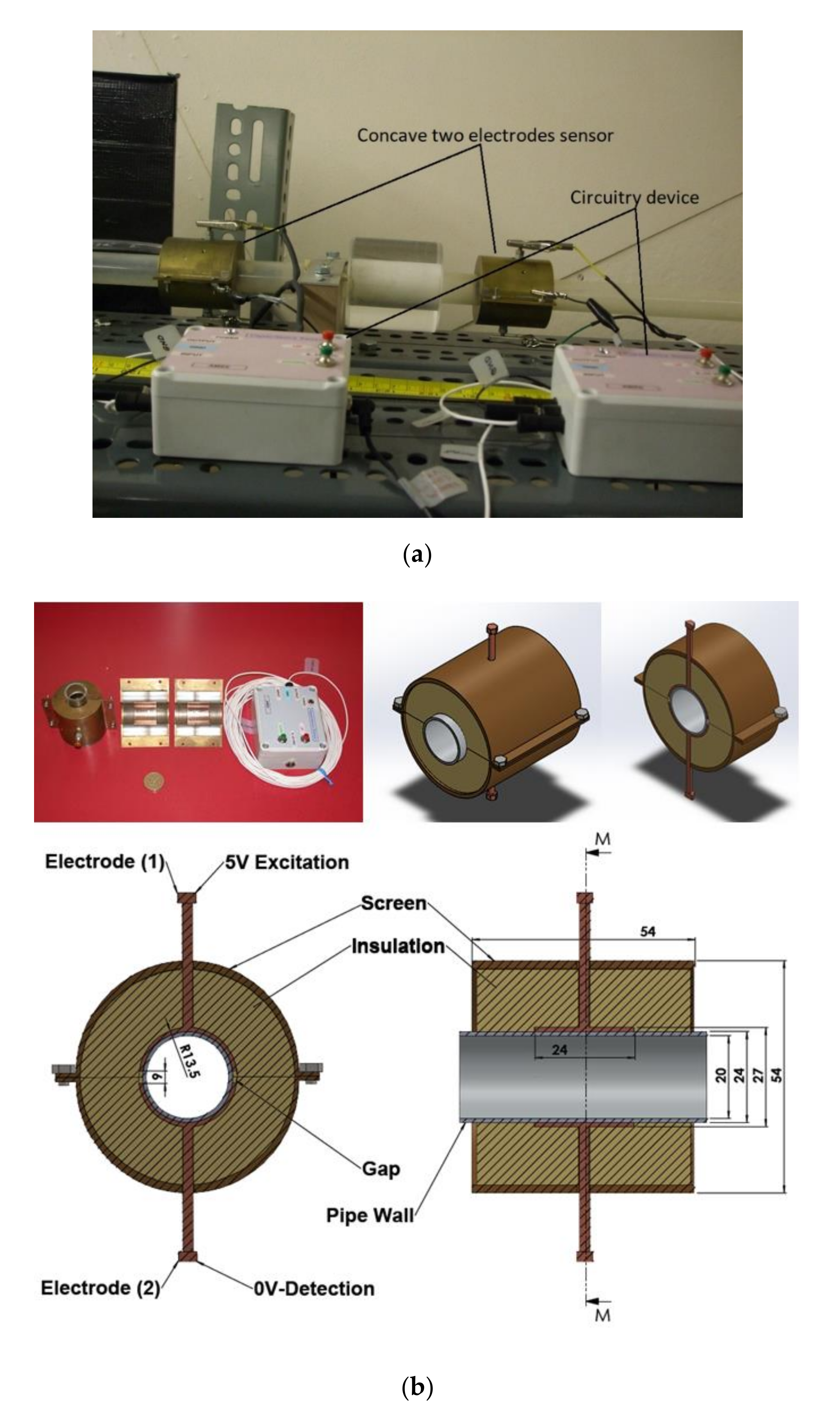
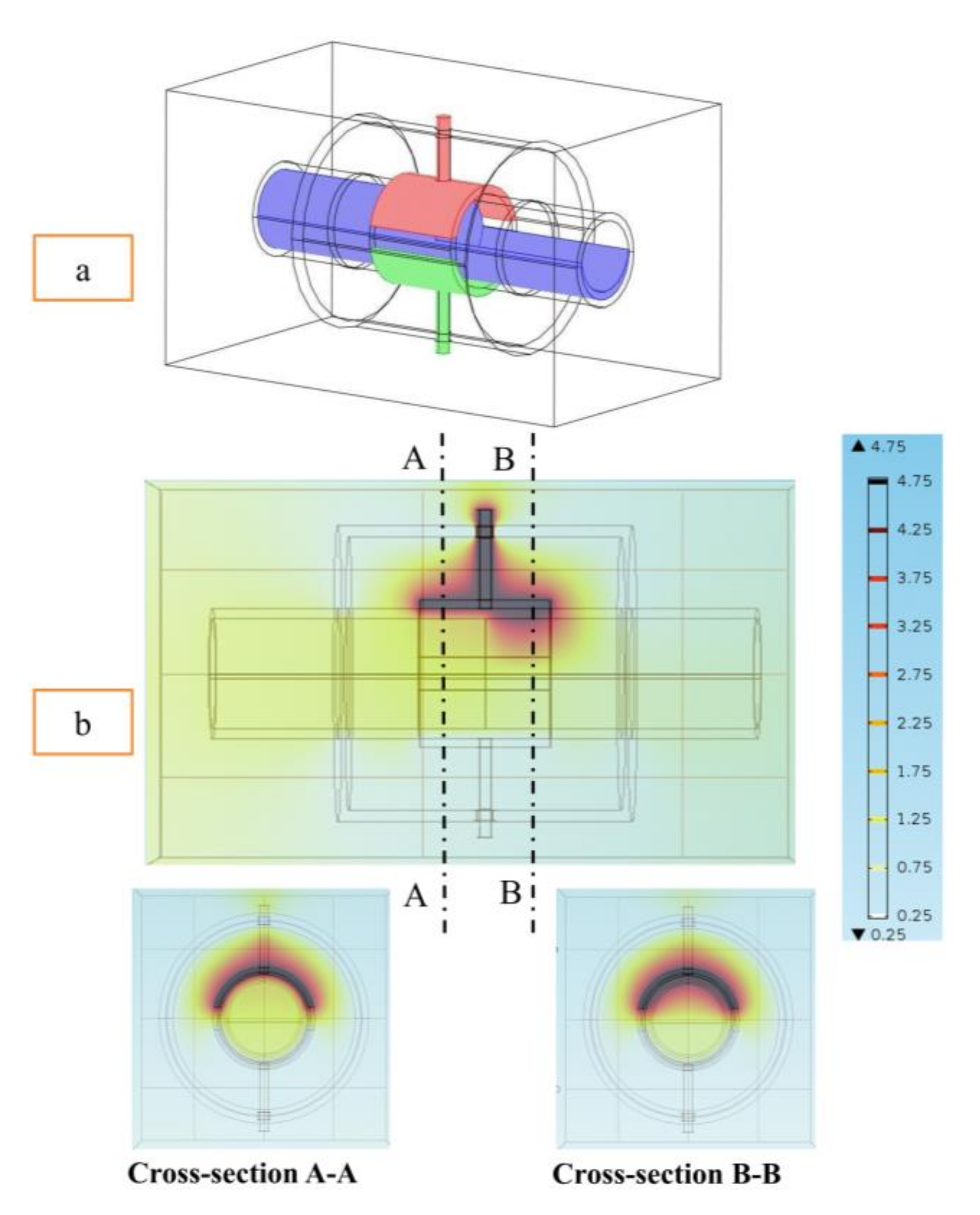
2. Experimental Apparatus and Methodology
3. Numerical Approach
- (a)
- For all the simulated flow patterns, the flow was advancing by 2 mm step until the entire structure of the flow pattern passed the capacitance sensor;
- (b)
- The period of time for the simulation was then taken as identical to the time elapsing in the real experiment while the same number of iterations of the flow pattern crossed the capacitance sensor;
- (c)
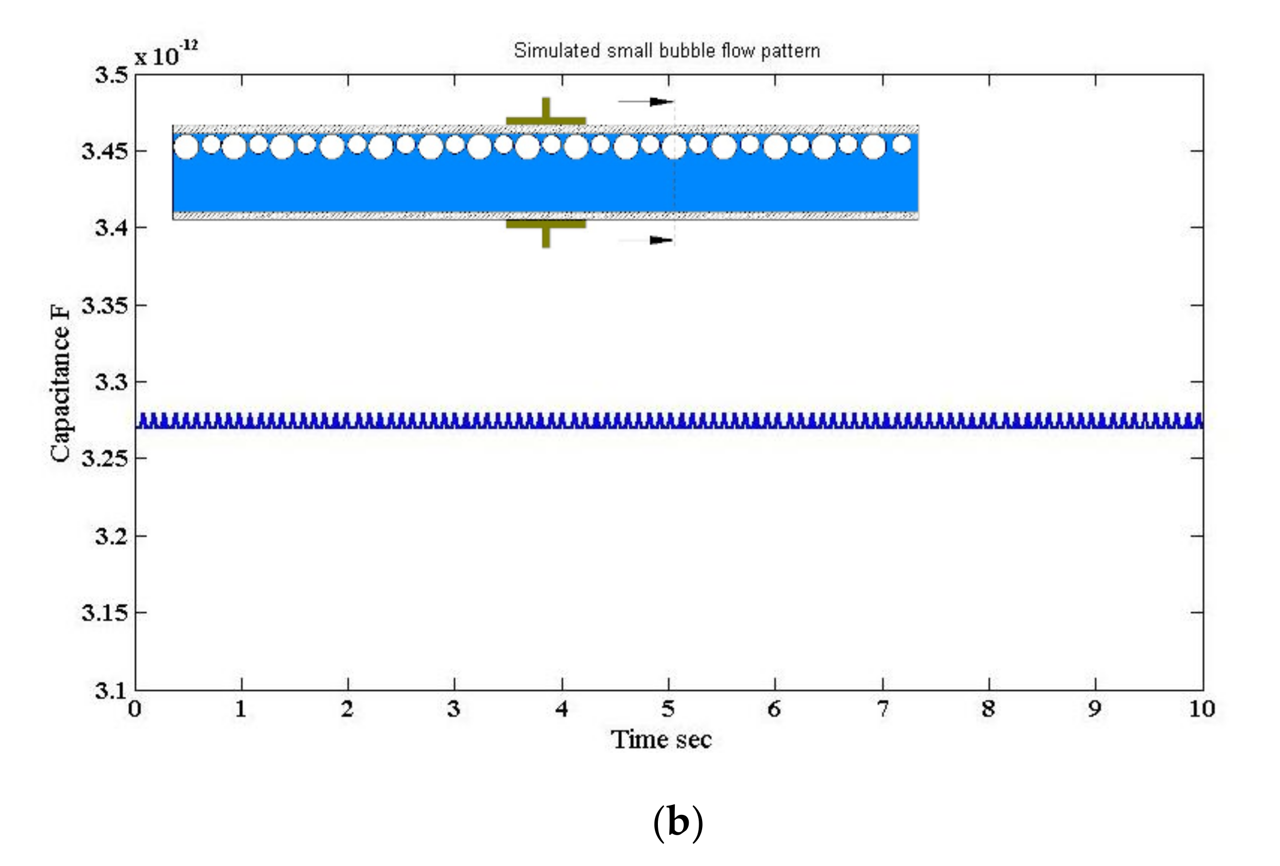
- In the small bubble flow pattern, the average sizes of the largest small bubbles and the smallest small bubbles were taken from the high-speed camera images;
- (d)
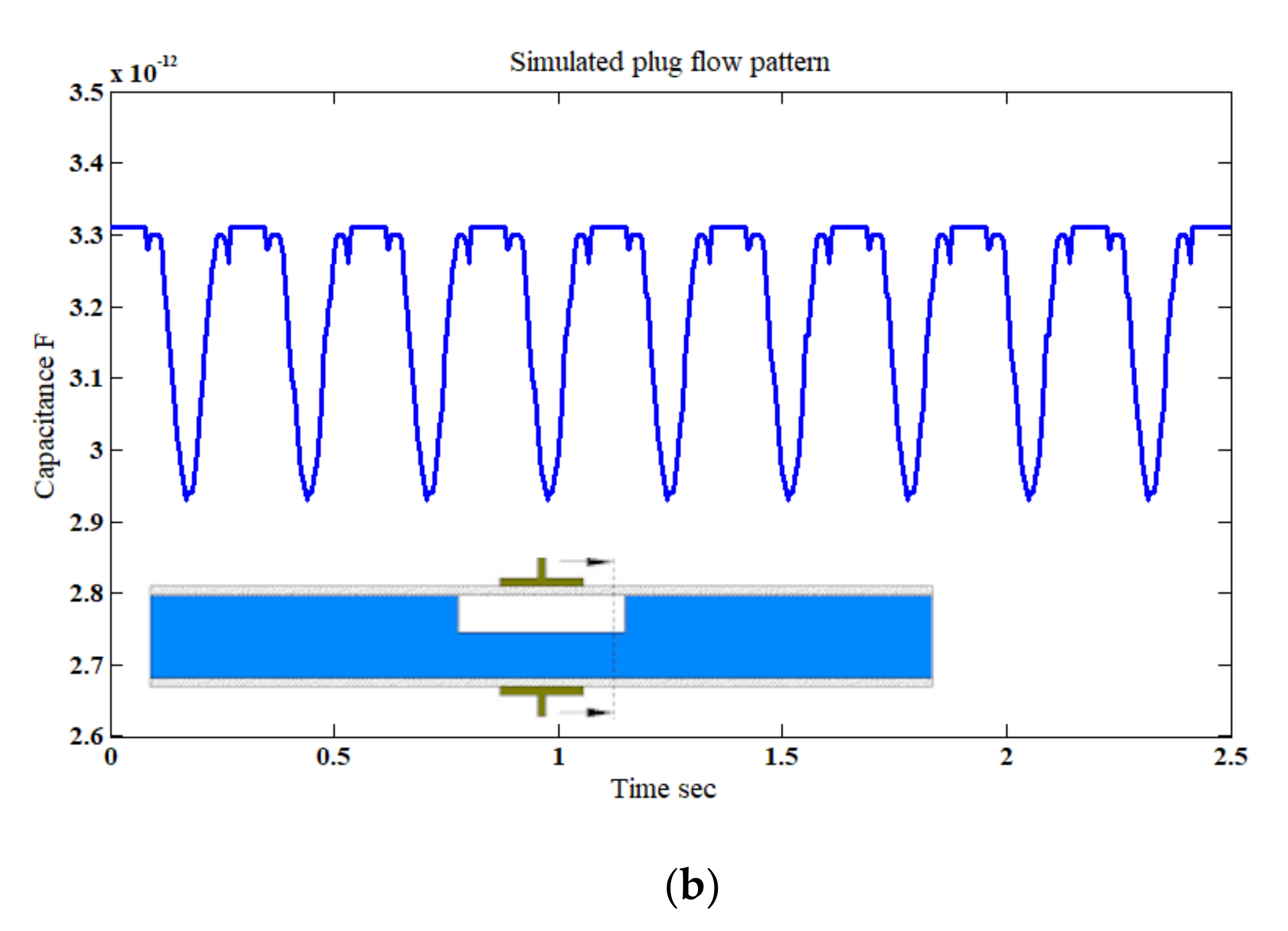
- The plug and elongated bubble flow patterns have the same hydrodynamic mechanism, however, the sizes of the bubbles are different;
- (e)
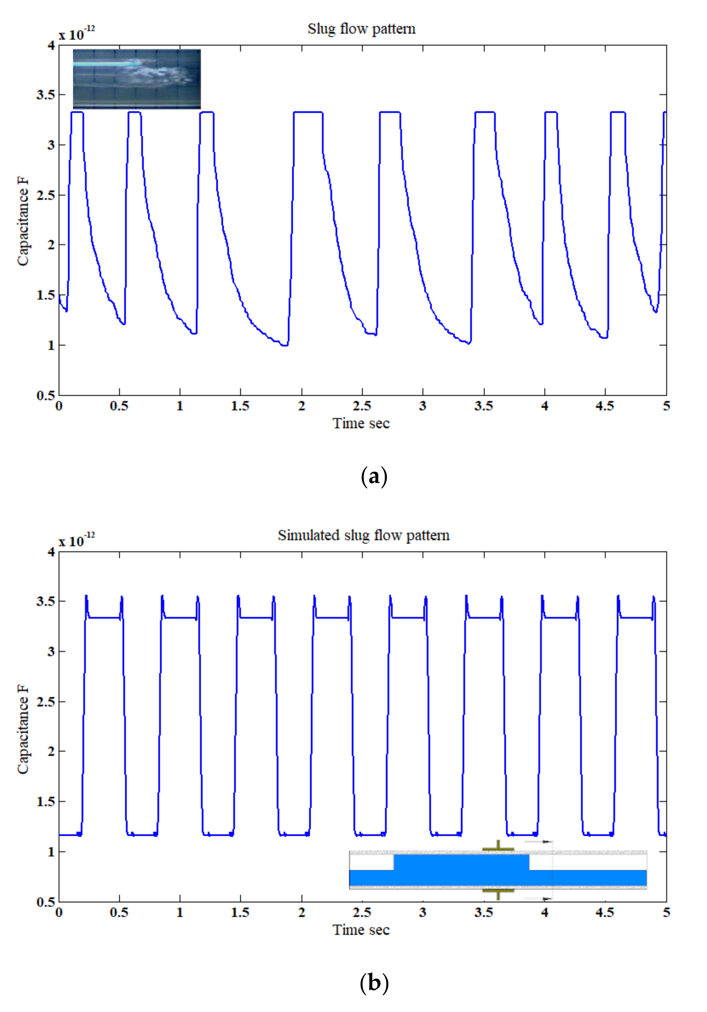
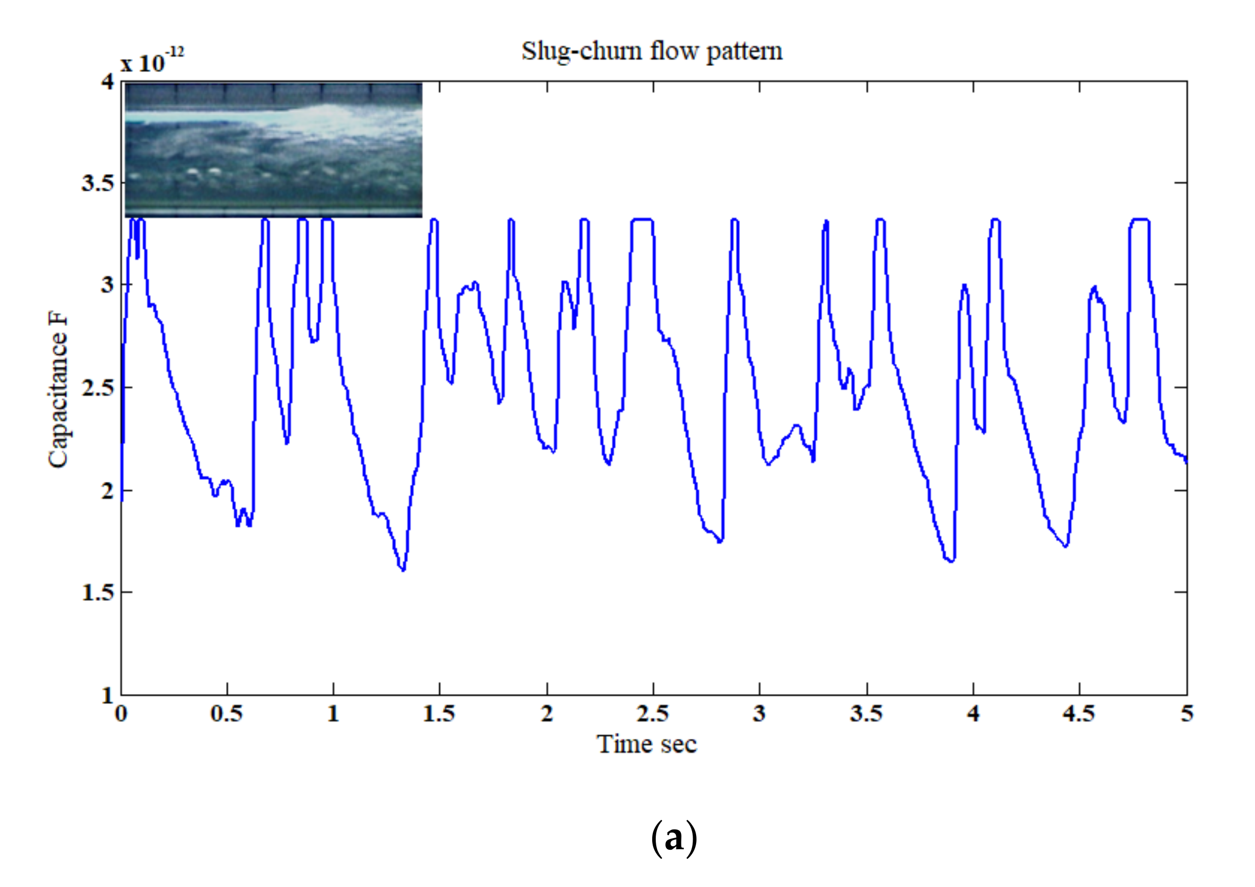
- The slug and slug–churn flow patterns have the same hydrodynamic mechanism, however, the slug–churn is frothier (this was implemented by having changing permittivity);
- (f)
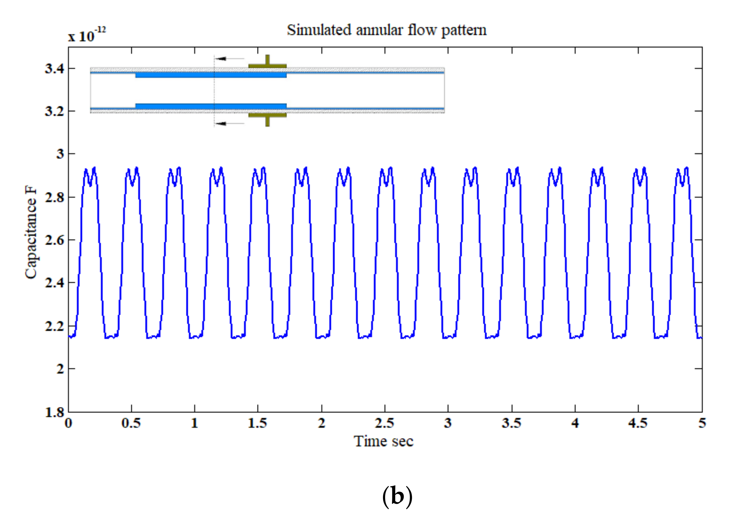
- For the annular flow pattern, the pipe wall was assumed to be wetted by a symmetrical liquid film of a thickness of 1 mm over the entire length of the model, except for the section before the capacitance sensor screen, where the thickness of the film was 3 mm, as the simulation was run, this thicker film advanced through the capacitance sensor in 2 mm steps until it filled the entire length of the model. The model assumed that the thickness of the liquid would be symmetric around the pipe;
- (g)
- Regardless of the inclination, the numerical model treated each flow pattern similarly for all inclinations. In other words, for example, the simulated small-bubbles/slug flow pattern is the same in structure for all inclination. The only two differences are (1) the combination of gas–liquid superficial velocities at which these flow patterns were induced due to the effect of gravity and inclination, and (2) some flow patterns did not form or develop in a certain inclination (i.e., the plug flow pattern at a horizontal 0°, and the stratified wavy at all upward inclined angles [28,32]).
4. Results and Discussion
4.1. Time Dependent Analysis
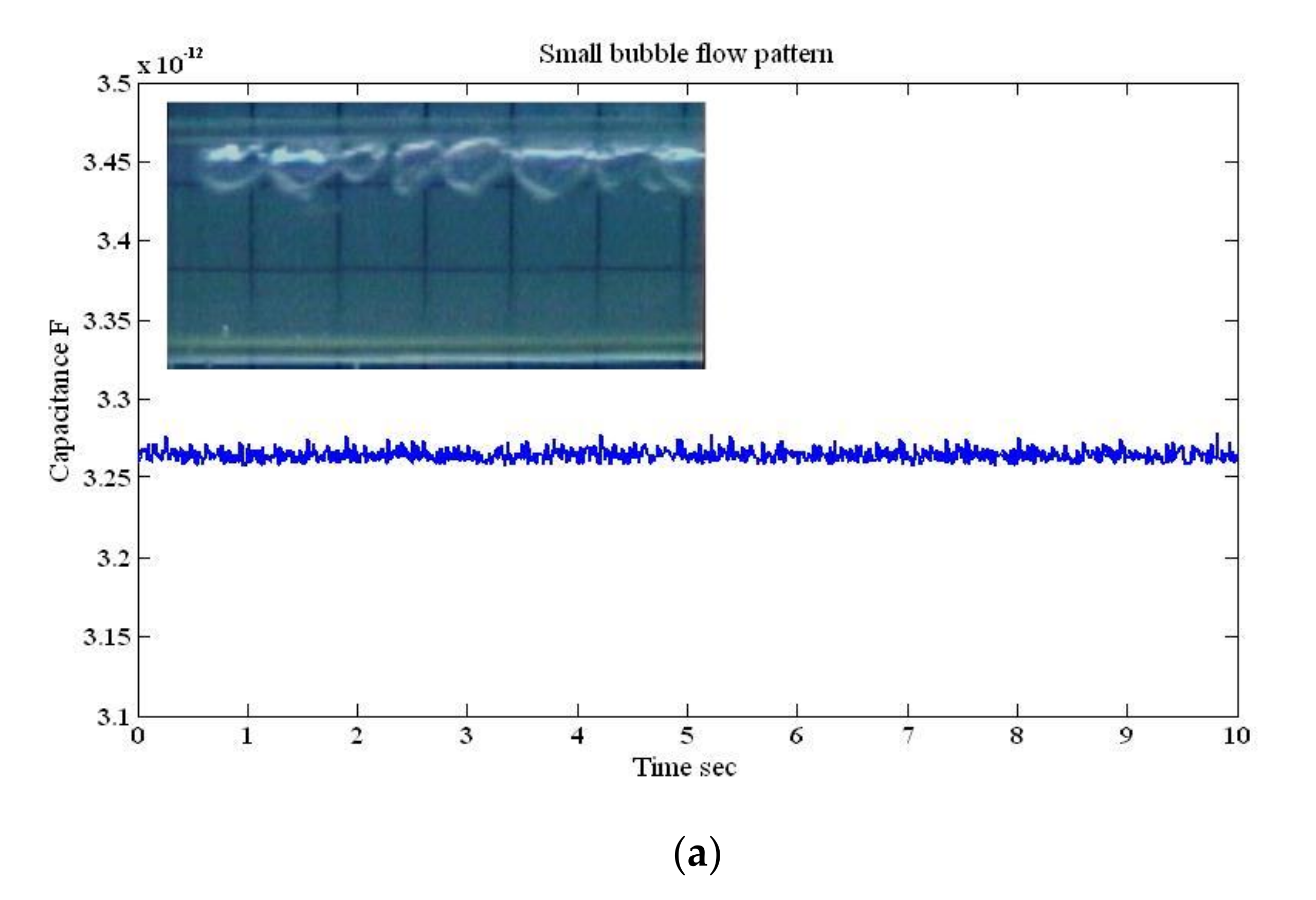
4.1.1. Small Bubble Flow Pattern
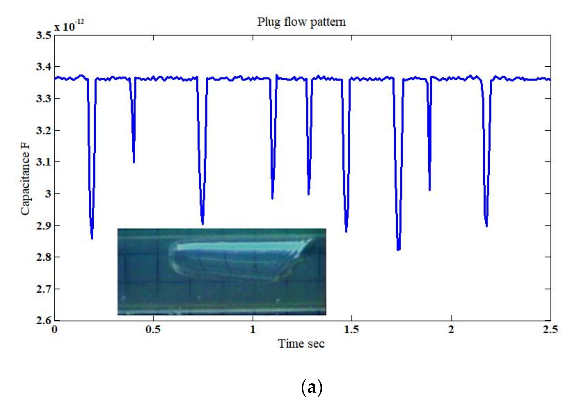
4.1.2. Plug and Elongated Flow Patterns
4.1.3. Slug and Slug–Churn Flow Patterns
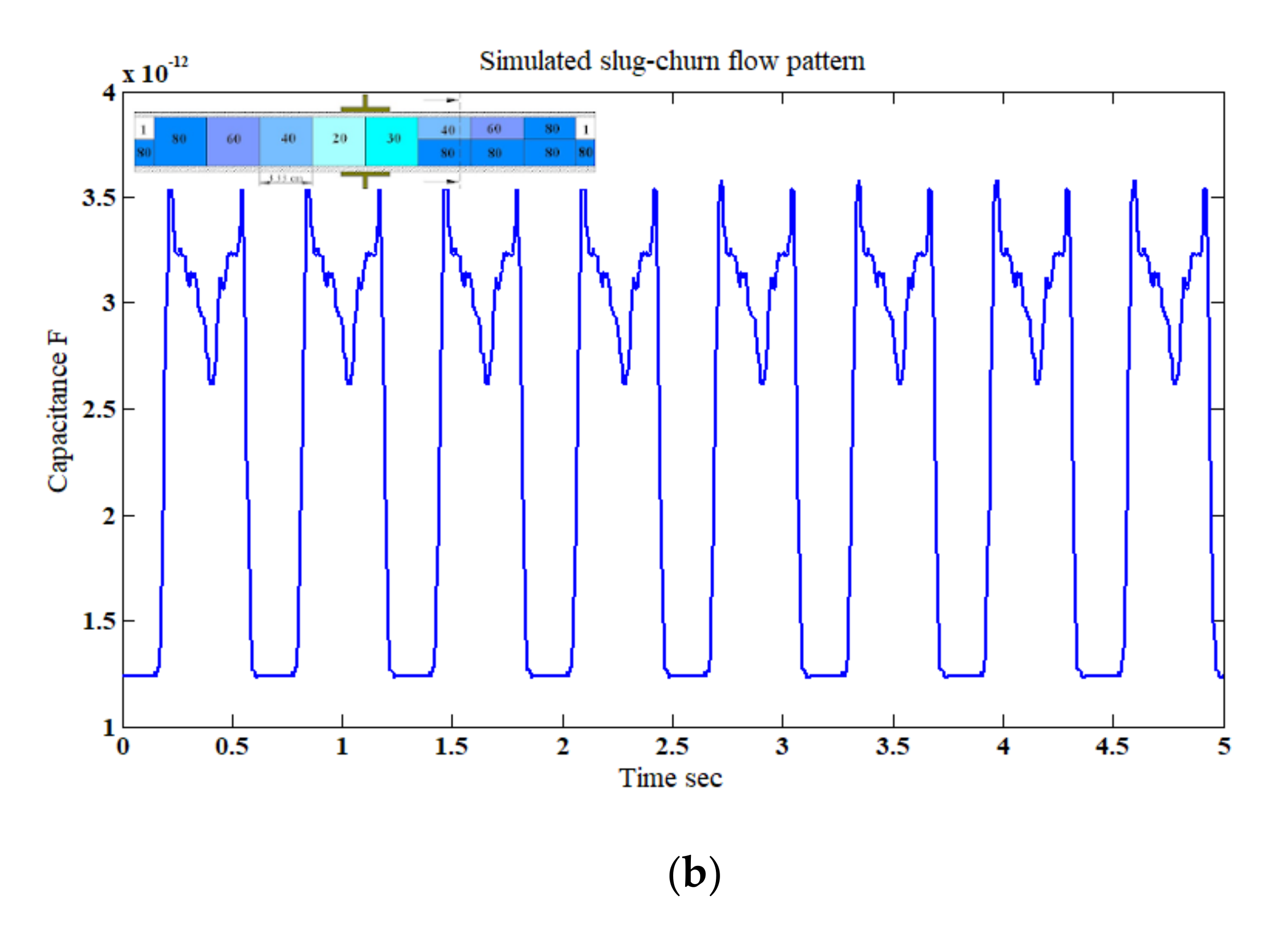
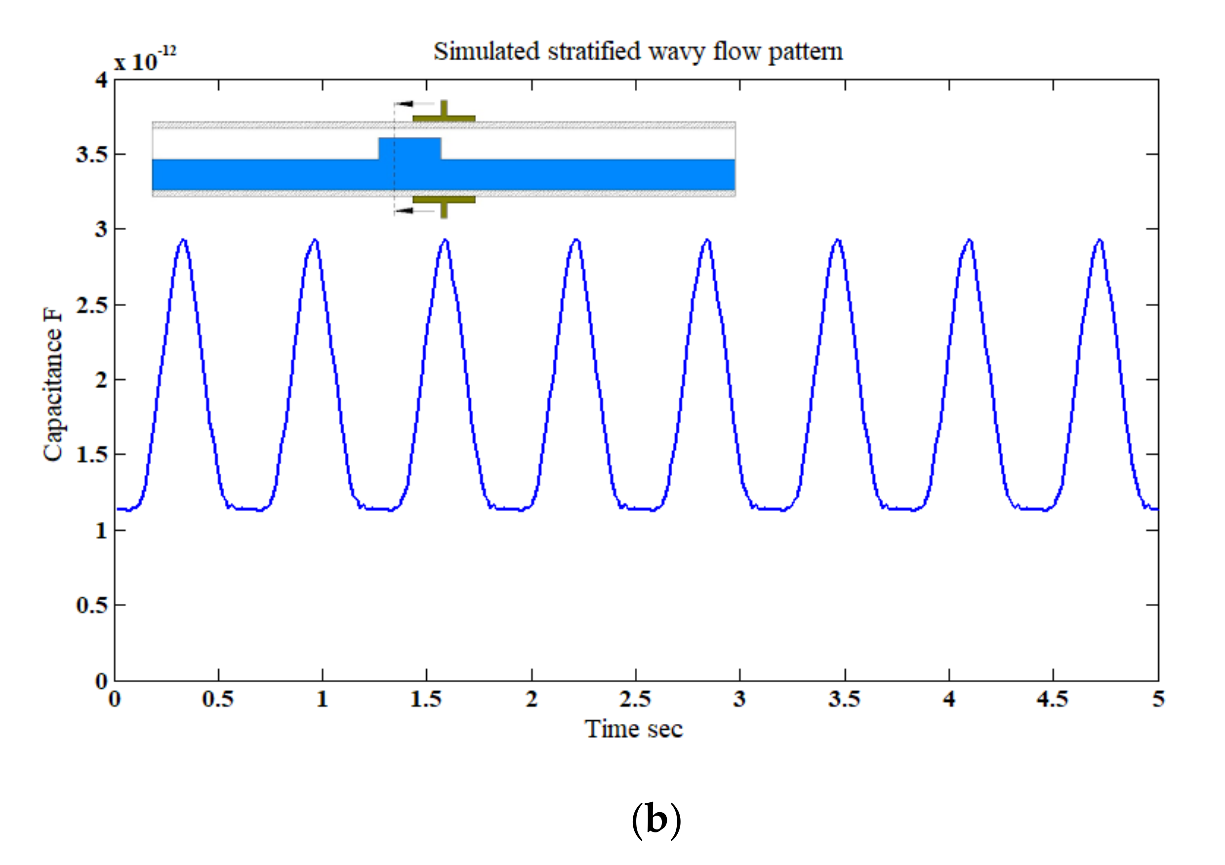
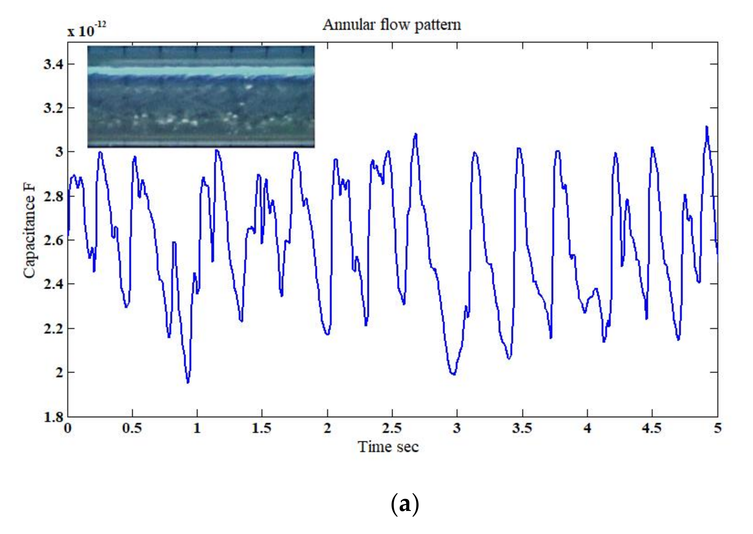
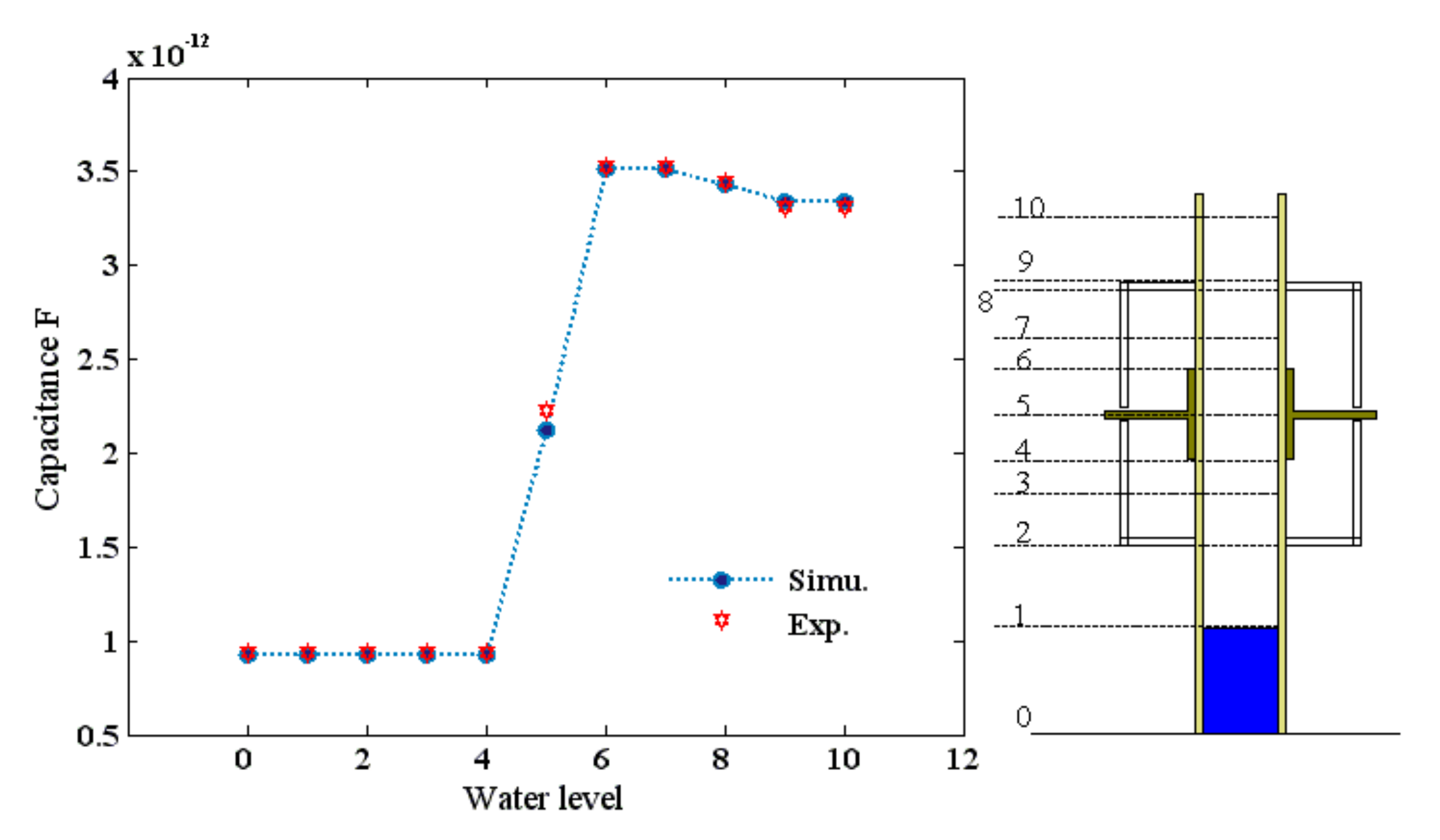
4.1.4. Stratified Wavy and Annular Flow Patterns
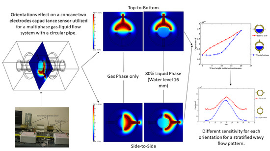
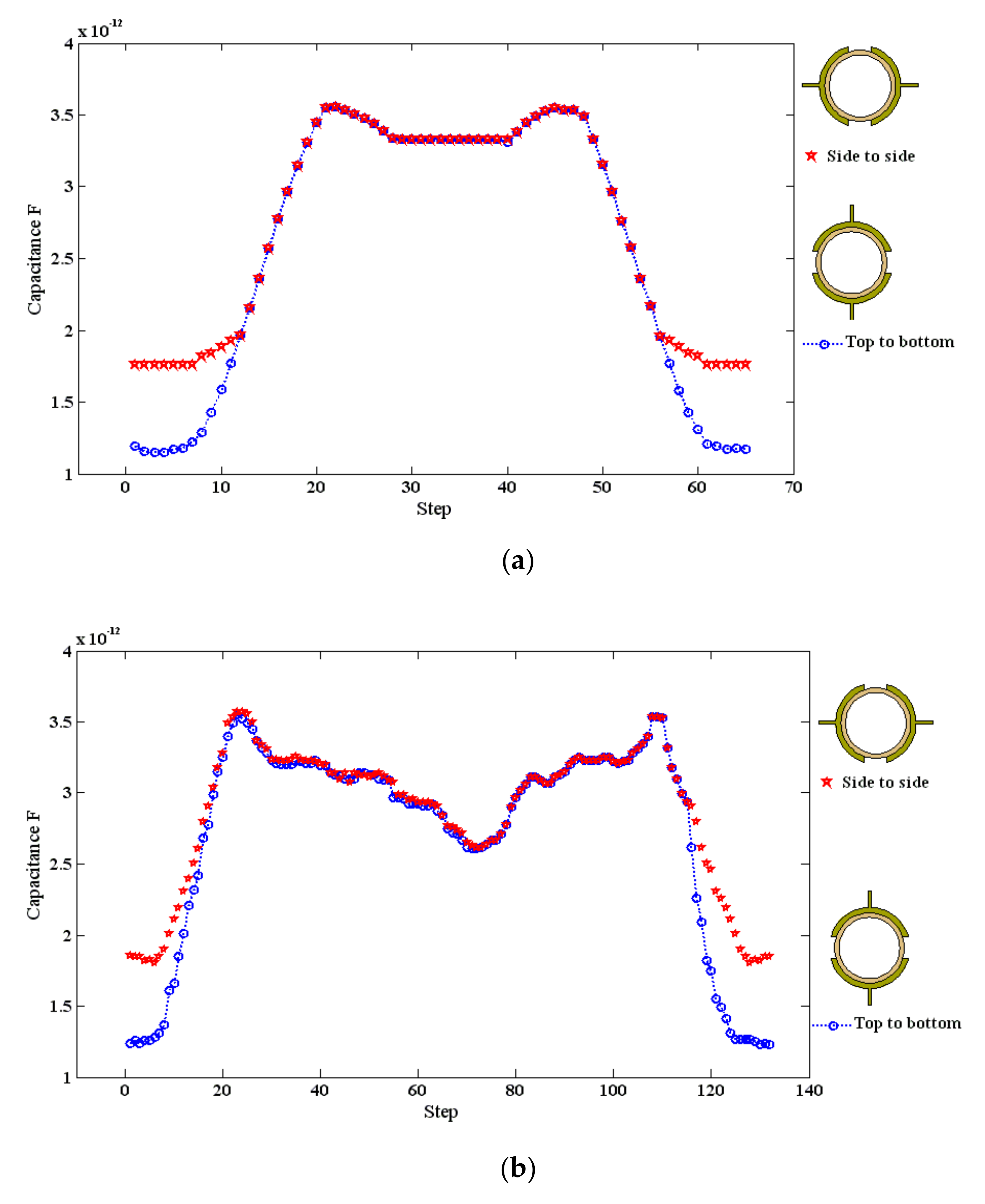
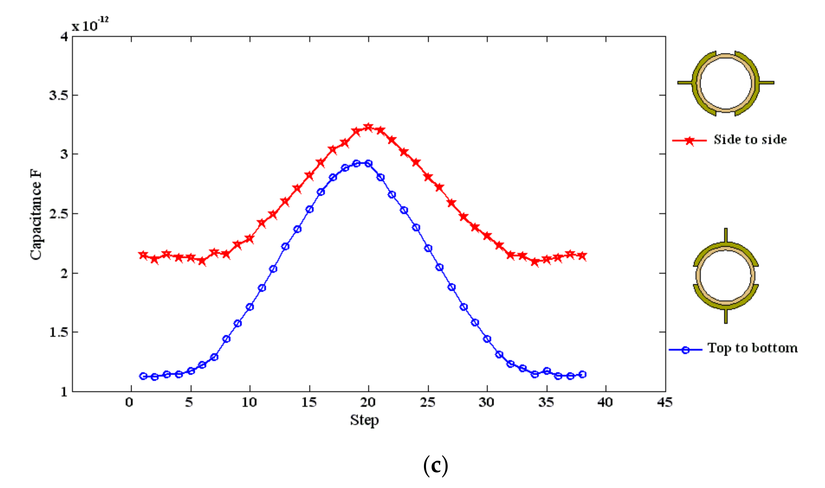
4.2. Optimizing Electrodes Orientation
5. Conclusions
Author Contributions
Funding
Acknowledgments
Conflicts of Interest
Nomenclature
| Latin Symbols | |
| C | Capacitance, pF |
| CG | Gas capacitance, pF |
| CL | Liquid capacitance, pF |
| CWall | Wall capacitance, pF |
| D | Electric displacement (vector), C/m2 |
| din | Inner pipe diameter, mm |
| dout | Outer pipe diameter, mm |
| da | Infinitesimal area on closed surface, m |
| E | Electrical field, V/m |
| n | A unit vector perpendicular to da, - |
| Q | Surface charge, C |
| S | Closed surface |
| uGS | Superficial gas velocity, m/s |
| uLS | Superficial liquid velocity, m/s |
| ut | Translational velocity, m/s |
| V(x,y,z) | Electric potential distribution, V |
| x(n) | Discrete time signal, units depend on application |
| Greek Symbols | |
| Permittivity of free space, F/m | |
| Permittivity distribution, - | |
| External charge density C/m3 | |
| Other Symbols | |
| Gradient operator | |
| Divergence operator | |
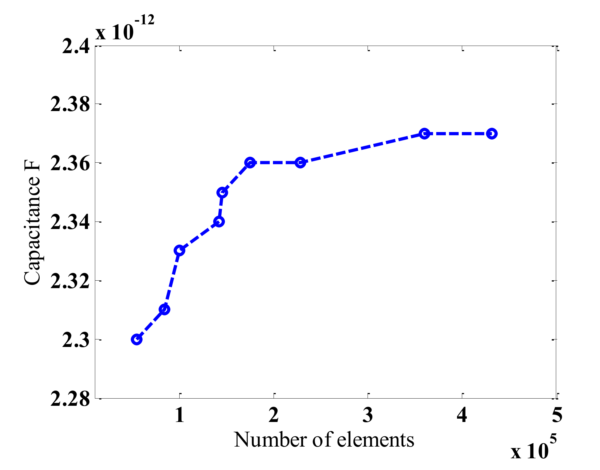
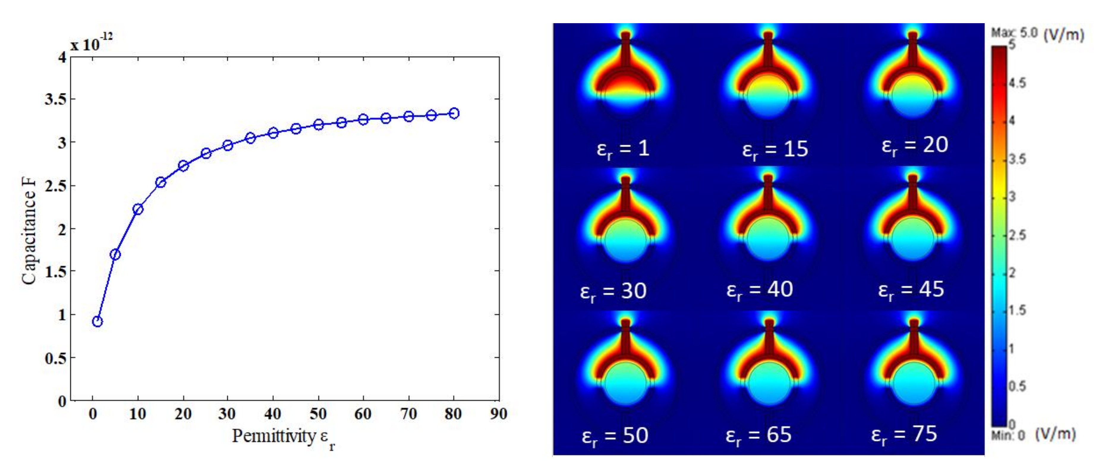
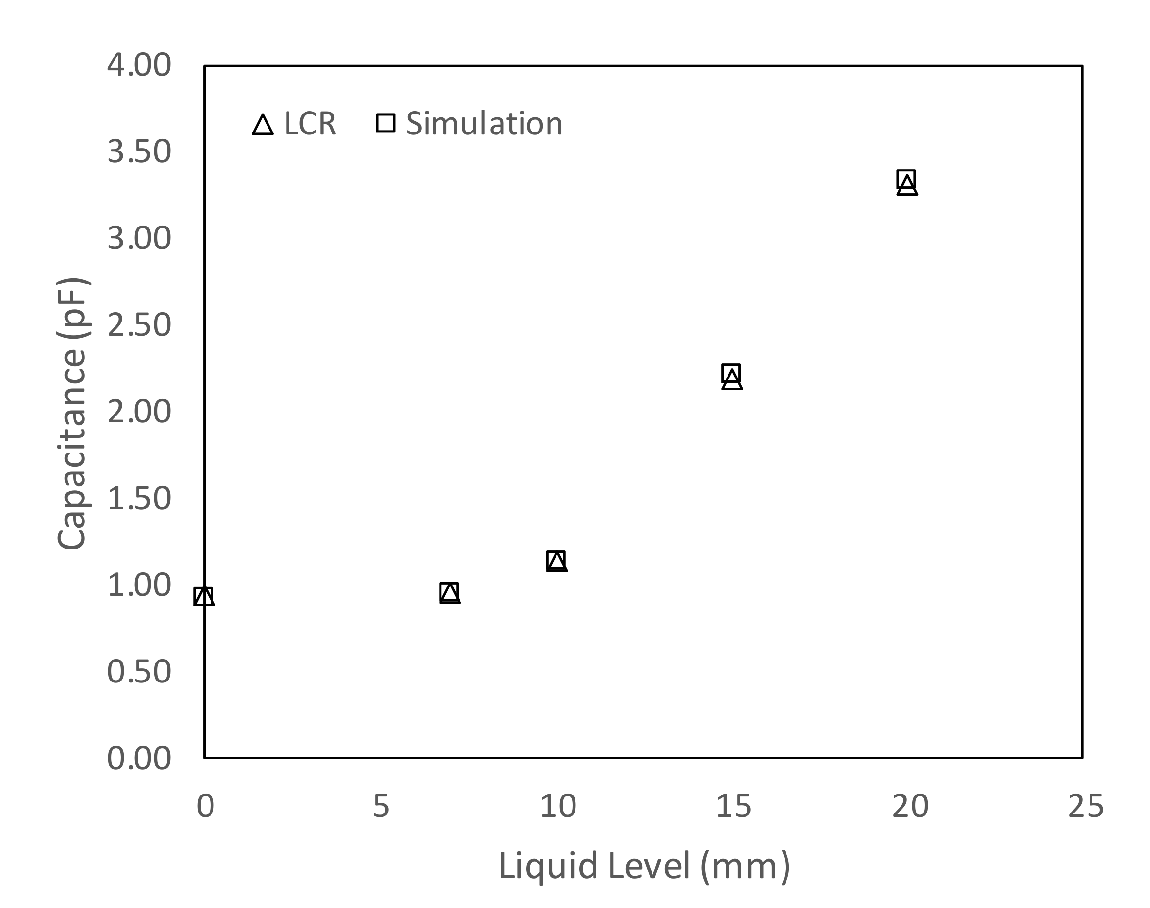
Appendix A
Numerical Model Spikes Rationale

References
- Alghamdi, Y.; Peng, Z.; Shah, K.; Moghtaderi, B.; Doroodchi, E. Predicting the solid circulation rate in chemical looping combustion systems using pressure drop measurements. Powder Technol. 2015, 286, 572–581. [Google Scholar] [CrossRef]
- Ludlow, J.C.; Monazam, E.R.; Shadle, L.J. Improvement of continuous solid circulation rate measurement in a cold flow circulating fluidized bed. Powder Technol. 2008, 182, 379–387. [Google Scholar] [CrossRef]
- Oki, K.; Akehata, T.; Shirai, T. A new method for measuring the velocity of solid particles with a fiber optic probe. Kagaku Kogaku 1973, 37, 965–967. [Google Scholar]
- Alghamdi, Y.A.; Doroodchi, E.; Moghtaderi, B. Mixing and segregation of binary oxygen carrier mixtures in a cold flow model of a chemical looping combustor. Chem. Eng. J. 2013, 223, 772–784. [Google Scholar] [CrossRef]
- Medrano, J.A.; De Nooijer, N.C.A.; Gallucci, F.; Van Sint Annaland, M. Advancement of an Infra-Red Technique for Whole-Field Concentration Measurements in Fluidized Beds. Sensors 2016, 16, 300. [Google Scholar] [CrossRef]
- Liu, R.; Zhou, Z.; Xiao, R.; Yu, A. CFD-DEM modelling of mixing of granular materials in multiple jets fluidized beds. Powder Technol. 2020, 361, 315–325. [Google Scholar] [CrossRef]
- Qureshi, A.E.; Creasy, D.E. Fluidised bed gas distributors. Powder Technol. 1979, 22, 113–119. [Google Scholar] [CrossRef]
- Alghamdi, A.Y.; Peng, Z.; Luo, C.; Almutairi, Z.; Moghtaderi, B.; Doroodchi, E. Systematic Study of Pressure Fluctuation in the Riser of a Dual Inter-Connected Circulating Fluidized Bed: Using Single and Binary Particle Species. Processes 2019, 7, 890. [Google Scholar] [CrossRef] [Green Version]
- Alghamdi, Y.; Peng, Z.; Moghtaderi, B.; Doroodchi, E. A correlation for predicting solids holdup in the dilute pneumatic conveying flow regime of circulating and interconnected fluidised beds. Powder Technol. 2016, 297, 357–366. [Google Scholar] [CrossRef]
- Amoresano, A.; Langella, G.; Di Santo, M.; Iodice, P. Advanced Imaging Techniques for Multiphase Flows Analysis. J. Phys. Conf. Ser. 2017, 882, 012004. [Google Scholar] [CrossRef]
- Ahmad, W.R.; Julio, M.D.J.; Masahiro, K. Falling film hydrodynamics in slug flow. Chem. Eng. Sci. 1998, 53, 123–130. [Google Scholar] [CrossRef]
- Kurada, S.; Rankin, G.W.; Sridhar, K. Flow visualization using photochromic dyes: A review. Opt. Lasers Eng. 1994, 20, 177–192. [Google Scholar] [CrossRef]
- Ayati, A.A.; Kolaas, J.; Jensen, A.; Johnson, G.W. A PIV investigation of stratified gas–liquid flow in a horizontal pipe. Int. J. Multiph. Flow 2014, 61, 129–143. [Google Scholar] [CrossRef] [Green Version]
- Albion, K.; Briens, L.; Briens, C.; Berruti, F.; Book, G. Flow regime determination in upward inclined pneumatic transport of particulates using non-intrusive acoustic probes. Chem. Eng. Process. 2007, 46, 520–531. [Google Scholar] [CrossRef]
- Prakash, B.; Parmar, H.; Shah, M.T.; Pareek, V.K.; Anthony, L.; Utikar, R.P. Simultaneous measurements of two phases using an optical probe. Exp. Comput. Multiph. Flow 2019, 1, 233–241. [Google Scholar] [CrossRef] [Green Version]
- Wang, G.; Ching, C.Y. Measurement of multiple gas-bubble velocities in gas-liquid flows using hot film anemometry. Exp. Fluids 2001, 31, 428–439. [Google Scholar] [CrossRef]
- Zhou, Y.; Jin, N.; Zhang, H.; Zhai, L. Method based on parallel-wire conductivity probe for measuring water hold-up in near-horizontal oil–water two-phase flow pipes. IET Sci. Meas. Technol. 2020, 14, 676–683. [Google Scholar] [CrossRef]
- Wang, D.; Jin, N.; Zhai, L.; Ren, Y. Measurement of Liquid Film Thickness Using Distributed Conductance Sensor in Multiphase Slug Flow. IEEE Trans. Ind. Electron. 2020, 67, 8841–8850. [Google Scholar] [CrossRef]
- Nydal, O.J.; Pintus, S.; Andreussi, P. Statistical characterization of slug flow in horizontal pipe. Int. J. Multiph. Flow 1992, 18, 439–453. [Google Scholar] [CrossRef]
- Jin, N.D.; Xin, Z.; Wang, J.; Wang, Z.Y.; Jia, X.H.; Chen, W.P. Design and geometry optimization of a conductivity probe with a vertical multiple electrode array for measuring volume fraction and axial velocity of two-phase flow. Meas. Sci. Technol. 2008, 19, 045403. [Google Scholar] [CrossRef]
- Williams, R.A.; Beck, M.S. Process Tomography Principle, Techniques and Applications; Butterworth-Heinemann Ltd.: Oxford, UK, 1995. [Google Scholar]
- Ismail, I.; Gamio, J.C.; Bukhari, S.F.A.; Yang, W.Q. Tomography for multi-phase flow measurement in the oil industry. Flow Meas. Instrum. 2005, 16, 145–155. [Google Scholar] [CrossRef]
- Kumar, S.B.; Duduković, M.P. Chapter 2—Computer assisted gamma and X-ray tomography: Applications to multiphase flow systems. In Non-Invasive Monitoring of Multiphase Flows; Chaouki, J., Larachi, F., Duduković, M.P., Eds.; Elsevier Science B.V.: Amsterdam, The Netherlands, 1997; pp. 47–103. [Google Scholar] [CrossRef]
- Kendoush, A.A. The Science and Technology of Void Fraction Measurements in Multiphase Flow. In Proceedings of the ASME-JSME-KSME 2019 8th Joint Fluids Engineering Conference, San Francisco, CA, USA, 28 July–1 August 2019. [Google Scholar]
- Xie, C.G.; Plaskowski, A.; Beck, M.S. 8-electrode capacitance system for two-component flow identification. I. Tomographic flow imaging. IEE Proc. A-Phys. Sci. Meas. Instrum. Manag. Educ. 1989, 136, 173–183. [Google Scholar] [CrossRef]
- Zhu, H.; Sun, J.; Xu, L.; Tian, W.; Sun, S. Permittivity Reconstruction in Electrical Capacitance Tomography Based on Visual Representation of Deep Neural Network. IEEE Sens. J. 2020, 20, 4803–4815. [Google Scholar] [CrossRef]
- Bahrami, B.; Mohsenpour, S.; Shamshiri Noghabi, H.R.; Hemmati, N.; Tabzar, A. Estimation of flow rates of individual phases in an oil-gas-water multiphase flow system using neural network approach and pressure signal analysis. Flow Meas. Instrum. 2019, 66, 28–36. [Google Scholar] [CrossRef]
- Almutairi, Z.; Al-Alweet, F.M.; Alghamdi, Y.A.; Almisned, O.A.; Alothman, O.Y. Investigating the Characteristics of Two-Phase Flow Using Electrical Capacitance Tomography (ECT) for Three Pipe Orientations. Processes 2020, 8, 51. [Google Scholar] [CrossRef] [Green Version]
- Jaworski, A.J.; Bolton, G.T. The design of an electrical capacitance tomography sensor for use with media of high dielectric permittivity. Meas. Sci. Technol. 2000, 11, 743–757. [Google Scholar] [CrossRef]
- Reinecke, N.; Mewes, D. Multielectrode capacitance sensors for the visualisation of transient two-phase flows. Exp. Therm. Fluid Sci. 1997, 15, 253–266. [Google Scholar] [CrossRef]
- Bangliang, S.; Zhang, Y.; Peng, L.; Yao, D.; Zhang, B. The use of simultaneous iterative reconstruction technique for electronic capacitance tomography. Chem. Eng. J. 2000, 77, 37–41. [Google Scholar] [CrossRef]
- Al-Alweet, F.M.; Jaworski, A.J.; Alghamdi, Y.A.; Almutairi, Z.; Kołłątaj, J. Systematic Frequency and Statistical Analysis Approach to Identify Different Gas–Liquid Flow Patterns Using Two Electrodes Capacitance Sensor: Experimental Evaluations. Energies 2020, 13, 2932. [Google Scholar] [CrossRef]
- Al-Alweet, F. The Development of Capacitance Measurement Techniques and Data Processing Methods for the Characterisation of Two-Phase Flow Phenomena in Horizontal and Inclined Pipelines. Ph.D. Thesis, The University of Manchester, Manchester, UK, 2008. [Google Scholar]
- Abouelwafa, M.S.A.; Kendall, E.J.M. The Use of Capacitance Sensors for Phase Percentage Determination in Multiphase Pipelines. IEEE Trans. Instrum. Meas. 1980, 29, 24–27. [Google Scholar] [CrossRef]
- Ferry, N.T. A Design Methodology for Low-Cost, High-Performance Capacitive Sensor. Ph.D. Thesis, Delft University of Technology, Delft, The Netherlands, 1997. [Google Scholar]
- Geraets, J.J.M.; Borst, J.C. A capacitance sensor for two-phase void fraction measurement and flow pattern identification. Int. J. Multiph. Flow 1988, 14, 305–320. [Google Scholar] [CrossRef]
- Beck, M.S.; Green, R.G.; Hammer, E.A.; Thorn, R. On-line measurement of oil/gas/water mixtures, using a capacitance sensor. Measurement 1985, 3, 7–14. [Google Scholar] [CrossRef]
- Canière, H.; T’Joen, C.; Willockx, A.; De Paepe, M. Capacitance signal analysis of horizontal two-phase flow in a small diameter tube. Exp. Therm. Fluid Sci. 2008, 32, 892–904. [Google Scholar] [CrossRef]
- Elkow, K.J.; Rezkallah, K.S. Void fraction measurements in gas-liquid flows using capacitance sensors. Meas. Sci. Technol. 1996, 7, 1153–1163. [Google Scholar] [CrossRef]
- Salehi, S.M.; Karimi, H.; Dastranj, A.A. A Capacitance Sensor for Gas/Oil Two-Phase Flow Measurement: Exciting Frequency Analysis and Static Experiment. IEEE Sens. J. 2017, 17, 679–686. [Google Scholar] [CrossRef]
- Stott, A.L.; Green, R.G.; Seraji, K. Comparison of the use of internal and external electrodes for the measurement of the capacitance and conductance of fluids in pipes. J. Phys. E Sci. Instrum. 1985, 18, 587–592. [Google Scholar] [CrossRef]
- Ahmed, W.; Fatayerji, A.; Elsaftawy, A.; Hassan, M.; Weaver, D.; Riznic, J. A New Capacitance Sensor for Measuring the Void Fraction of Two-Phase Flow Through Tube Bundles. Sensors 2020, 20, 2088. [Google Scholar] [CrossRef] [Green Version]
- Tollefesn, J.; Hammer, E. Capacitance sensor design for reducing errors in phase concentration measurements. Flow Meas. Instrum. 1998, 9, 25–32. [Google Scholar] [CrossRef]
- Hammer, E.A.; Green, R.G. The spatial filtering effect of capacitance transducer electrodes. J. Phys. E Sci. Instrum. 1983, 16, 438–443. [Google Scholar] [CrossRef]
- Heerens, W.C. Application of capacitance techniques in sensor design. J. Phys. E Sci. Instrum. 1986, 19, 897–906. [Google Scholar] [CrossRef]
- Tapp, H.S.; Peyton, A.J.; Kemsley, E.K.; Wilson, R.H. Chemical engineering applications of electrical process tomography. Sens. Actuators B Chem. 2003, 92, 17–24. [Google Scholar] [CrossRef]
- Gamio, J.C.; Castro, J.; Rivera, L.; Alamilla, J.; Garcia-Nocetti, F.; Aguilar, L. Visualisation of gas-oil two-phase flows in pressurised pipes using electrical capacitance tomography. Flow Meas. Instrum. 2005, 16, 129–134. [Google Scholar] [CrossRef]
- Zhang, M.; Soleimani, M. Simultaneous reconstruction of permittivity and conductivity using multi-frequency admittance measurement in electrical capacitance tomography. Meas. Sci. Technol. 2016, 27, 025405. [Google Scholar] [CrossRef] [Green Version]
- Canière, H.; T’Joen, C.; Willockx, A.; Paepe, M.D.; Christians, M.; Rooyen, E.v.; Liebenberg, L.; Meyer, J.P. Horizontal two-phase flow characterization for small diameter tubes with a capacitance sensor. Meas. Sci. Technol. 2007, 18, 2898–2906. [Google Scholar] [CrossRef]
- Lim, L.G.; Tang, T.B. Design of concave capacitance sensor for void fraction measurement in gas-liquid flow. In Proceedings of the 2016 8th International Conference on Information Technology and Electrical Engineering (ICITEE), Yogyakarta, Indonesia, 5–6 October 2016; pp. 1–5. [Google Scholar]
- Thorncroft, G.E.; Klausner, J.F. A Capacitance Sensor for Two-Phase Liquid Film Thickness Measurements in a Square Duct. J. Fluids Eng. 1997, 119, 164–169. [Google Scholar] [CrossRef]
- Kwak, H.; Ke, H.; Lee, B.H.; Hubing, T. Plate Orientation Effect on the Inductance of Multi-Layer Ceramic Capacitors. In Proceedings of the 2007 IEEE Electrical Performance of Electronic Packaging, Atlanta, GA, USA, 29–31 October 2007; pp. 95–98. [Google Scholar]
- Kollataj, J. Capacitance Measurement System for Flow Pattern Detection In gas-liquid Flow in The Industrial Environment With Electromagnetic Interferences. In Proceedings of the XVIII-th International Conference on Electromagnetic Disturbances, Vilnius, Lithuania, 25–26 September 2008; pp. 133–136. [Google Scholar]
- Kollataj, J. The Multi-Channel Capacitance Unit for the Interface Level and Flow Sensors Sensitive to Electromagnetic Interferences; AMEX; AMEX Research Corporation Technologies: Bialystok, Poland, 2008. [Google Scholar]
- COMSOL. COMSOL Multiphysics-Electromagnetic-The Electrostatics Application Mode, 3.2b; COMSOL AB: London, UK, 2006. [Google Scholar]
- Reitz, J.R.; Milford, F.J.; Christy, R.W. Foundation of Electromagnetic Theory; Addison-Wesley Publishing Company: New York, NY, USA, 1993; pp. 50–153. [Google Scholar]
- Crowley, J.M. Fundamentals of Applied Electrostatics; A Wiley-Interscience Publication: New York, NY, USA, 1986; pp. 3–55. [Google Scholar]


| Type of Sensor | Principle of Work | Usefulness |
|---|---|---|
| High-speed camera images ([10]) |
|
|
| Photochromic dye activation ([11,12]) |
|
|
| Particles image velocimetry (PIV) ([13]) |
|
|
| Acoustic techniques ([14]) |
|
|
| Optical fiber probes ([15]) |
|
|
| Two hot film anemometers ([16]) |
|
|
| Conductivity and conductance probes ([17,18,19,20]) |
|
|
| Tomographic methods ([21,22,23,24,25,26]) |
|
|
| Static/differential pressure ports ([27]) |
|
|
| Component | Dimension | Specification |
|---|---|---|
| Test section | l = 4 m, din = 20 mm, and dout = 24 mm | Transparent acrylic pipe |
| Air compressor system | Brass pipe, l = 2.50 m, and din = 9.0 mm | - |
| A metering system to the supply air | - |
|
| Turbine flowmeter | - | FTB790-Omega, accuracy of ±0.2% |
| Gas–liquid mixer | l = 280 mm, internal pipe din = 20 mm | 100 holes, 1 mm in diameter, dispersed 10 mm apart in the axial direction and 5 mm away from each other on the circumference |
| Swing table | - | Inclination range from 0° to 30° |
| High-speed camera images | 2 min, shutter speed = 1/10,000 s, frame rate = 500/s | Installed at 3.4 m after the inlet of the test section |
| Tank | V1 = of 0.288 m3 (main) V2 = of 0.166 m3 (return) | - |
| Submersible pump | - | 70 L/min |
| Capacitance sensor (two electrodes [32]) | din = 24 mm, dout = 54 mm, l = 54 mm, gap between electrodes = 6 mm, insulation l = 50 mm, and brass screen thickness = 2 mm | C1 at 3 m and C2 at 3.25 m from the inlet |
| Flow Pattern Type | Inclination | |||||
|---|---|---|---|---|---|---|
| Horizontal 0° | Upward 15° | Upward 30° | ||||
| Range of Gas–Liquid Phases Superficial Velocities (m/s) | ||||||
| Gas Phase | Liquid Phase | Gas Phase | Liquid Phase | Gas Phase | Liquid Phase | |
| Small bubbles | 0.040–0.050 | 0.70–1.1 | 0.035–0.048 | 0.318–1.1 | 0.025–0.065 | 0.425–1.1 |
| Plug * | N/A | N/A | 0.127–0.50 | 0.53–1.1 | 0.051–0.314 | 0.21–1.1 |
| Elongated bubbles | 0.15–0.74 | 0.42–1.1 | 0.25–0.75 | 0.32–1.1 | 0.055–0.576 | 0.11–1.1 |
| Slug | 0.37–2.29 | 0.316–1.1 | 0.70–2.18 | 0.12–1.1 | 0.47–2.86 | 0.11–0.95 |
| Slug–churn | 2.11–3.74 | 0.425–1.1 | 2.90–4.40 | 0.11–1.1 | 2–4.29 | 0.10–1.1 |
| Annular | 4.48–5 | 0.31–1.1 | 4.75-5 | 0.106–1.1 | 4–5 | 0.11–1.1 |
| Stratified wavy * | 1.24–3 | 0.1–0.32 | N/A | N/A | N/A | N/A |
| Type of Flow Pattern | Arrangement | Cross-Sectional View | Explanation | Number of Times Passed the Capacitance Sensor | 3D Demonstration of the Defined Model Geometry |
|---|---|---|---|---|---|
| Small bubble |  |  | 2 different sizes of small spherical bubble | 100 in 10 s |  |
| Plug |  |  | Cylindrical bubble | 9 times, 9 cap bubbles in 3 s |  |
| Elongated bubble |  |  | Large cylindrical bubble | 15 times, 15 elongated bubbles in 4 s |  |
| Slug |  |  | Start with a concave-shaped liquid at bottom, and later a pipe filled with liquid phase | 8 times, 8 slugs in 5 s |  |
| Slug–churn |  |  | Pipe divided into 8 different permittivity sections | 8 times, 8 slug–churns in 5 s |  |
| Annular |  |  | Symmetrical liquid film of thickness 1 mm, then increased by 2 mm | 15 times, 15 spikes in 5 s |  |
| Stratified |  |  | Starts with liquid up to the midline of the pipe, then a square wave of liquid crosses the sensor | 8 times, 8 waves in 5 s |  |
© 2020 by the authors. Licensee MDPI, Basel, Switzerland. This article is an open access article distributed under the terms and conditions of the Creative Commons Attribution (CC BY) license (http://creativecommons.org/licenses/by/4.0/).
Share and Cite
Al-Alweet, F.M.; Jaworski, A.J.; Alghamdi, Y.A.; Almutairi, Z.; Kołłątaj, J. A Simplified Numerical Approach to Examine the Sensitivity of Two-Electrode Capacitance Sensor Orientation to Capture Different Gas–Liquid Flow Patterns in a Small Circular Pipe. Sensors 2020, 20, 4971. https://doi.org/10.3390/s20174971
Al-Alweet FM, Jaworski AJ, Alghamdi YA, Almutairi Z, Kołłątaj J. A Simplified Numerical Approach to Examine the Sensitivity of Two-Electrode Capacitance Sensor Orientation to Capture Different Gas–Liquid Flow Patterns in a Small Circular Pipe. Sensors. 2020; 20(17):4971. https://doi.org/10.3390/s20174971
Chicago/Turabian StyleAl-Alweet, Fayez M., Artur J. Jaworski, Yusif A. Alghamdi, Zeyad Almutairi, and Jerzy Kołłątaj. 2020. "A Simplified Numerical Approach to Examine the Sensitivity of Two-Electrode Capacitance Sensor Orientation to Capture Different Gas–Liquid Flow Patterns in a Small Circular Pipe" Sensors 20, no. 17: 4971. https://doi.org/10.3390/s20174971