

Construction of Aerosol Model and Atmospheric Correction in the Coastal Area of Shandong Peninsula


1
National Satellite Ocean Application Service, Beijing 100081, China
2
National Marine Environmental Forecasting Center, Beijing 100081, China
3
School of Environment, Southern University of Science and Technology, Shenzhen 518055, China
*
Author to whom correspondence should be addressed.
Remote Sens. 2024, 16(7), 1309; https://doi.org/10.3390/rs16071309
Submission received: 22 February 2024
/
Revised: 1 April 2024
/
Accepted: 3 April 2024
/
Published: 8 April 2024
(This article belongs to the Special Issue Aerosol and Atmospheric Correction)
Abstract
:Applying standard aerosol models for atmospheric correction in nearshore coastal waters introduces significant uncertainties due to their inability to accurately represent aerosol characteristics in these regions. To improve the accuracy of remote sensing reflectance () products in the nearshore waters of the Shandong Peninsula, this study develops an aerosol model based on aerosol data collected from the Mu Ping site in the coastal area of the Shandong Peninsula, enabling tailored atmospheric correction for this specific region. Given the pronounced seasonal variations in aerosol optical properties, monthly aerosol models were developed. The monthly aerosol model is derived using the average values of aerosol microphysical properties. Compared to the standard aerosol model, this model is more effective in characterizing the absorption and scattering characteristics of aerosols in the study area. Corresponding lookup tables for the aerosol model were created and integrated into the NIR-SWIR atmospheric correction algorithm. According to the accuracy evaluation indexes of RMSD, MAE, and UPD, it can be found that the atmospheric correction results of the aerosol model established in this paper are better than those of the standard aerosol model, especially in the 547 nm band. It demonstrates that the new aerosol model outperforms the standard model in atmospheric correction performance. With the increasing availability of aerosol observational data, the aerosol model is expected to become more accurate and applicable to other satellite missions.

1. Introduction
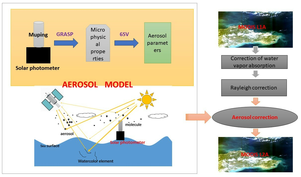
Ocean color remote sensing provides abundant observational data for studying water color constituents, including chlorophyll-a concentration, suspended sediment concentration, and water transparency [1,2]. These water color constituents can be inferred using inversion algorithms constructed with remote sensing reflectance () at different spectral bands as variables. Remote sensing reflectance is typically defined as the ratio of radiance leaving the water () to the downwelling irradiance just above the water surface (). The signal outside the water constitutes only a small fraction of the signal received by the satellite, with the majority originating from interactions with aerosols and Rayleigh molecules. This atmospheric signal contributes approximately 80% to 90% of the satellite signal in the visible light spectrum over the ocean [3,4]. Additionally, it is subject to subtle influences such as glint and whitecaps. Therefore, obtaining accurate water-leaving signals requires the crucial step of mitigating the impact of aerosols and Rayleigh molecules. Due to the relatively stable composition of molecules in the atmosphere, the portion of Rayleigh molecular scattering can be accurately assessed by considering the influences of polarization, surface pressure, and roughness [5,6]. It is evident from this that mitigating the impact of aerosol components is particularly crucial for obtaining accurate water-leaving signals. As is well known, atmospheric aerosol properties exhibit significant variability across both temporal and spatial scales. Differences in geographical location and time can lead to pronounced disparities in aerosol optical and microphysical characteristics [7]. Consequently, developing an appropriate aerosol model for the relevant satellite images is crucial for eliminating aerosol signals and achieving effective atmospheric correction [8].
The microphysical and optical properties of aerosols, such as particle size distribution and complex refractive index, effectively characterize the features of regional aerosols. They contribute to the successful elimination of aerosol signals during atmospheric correction processes, thus obtaining accurate products [9]. However, characterizing these aerosol properties proves challenging due to their significant temporal and spatial variability [10]. To improve this situation, many studies began analyzing various aerosol observational data to characterize aerosol properties. By constructing different aerosol models, they aim to characterize the absorption and scattering characteristics of aerosols under different temporal and spatial conditions [11,12,13].
Aerosol particle size distribution is an important indicator for studying the origin and distribution of aerosols, and it is commonly incorporated as one of the aerosol model parameters [14,15]. The aerosol size distribution is commonly characterized using the classical log-normal distribution theory, which assigns specific parameters to each component, including modal radius and standard deviation [16]. Several other studies utilize power functions, gamma functions, and analytical functions to depict aerosol particle sizes and their distribution [17,18,19,20]. Based on size distribution, aerosols are classified into five categories (rural, urban, maritime, tropospheric, and fog) by Shettle and Fenn, commonly known as SF79 [12]. In establishing relevant aerosol models, they further consider the impact of relative humidity on each group of aerosol particles. Gordon and Wang [21] were the first to apply three SF79 aerosol models (maritime, coastal, and tropospheric) in atmospheric correction for ocean color remote sensing satellite imagery. Chomko and Gordon introduced maritime, coastal, tropospheric, and urban aerosol models [17].
Ahmad et al. [22] categorized aerosol types into 10 categories and combined them with eight relative humidity levels to form 80 aerosol models (referred to as AF10). They constructed corresponding lookup tables for each model. Among these, the fine-mode particle component of the 10 aerosol types is comprised of 99.5% dust particles and 0.5% soot particles, showing excellent consistency with the average results of aerosol optical properties measured by AERONET. These 10 aerosol models have varying proportions of coarse and fine modal particles but share the same effective radius and mean radius [5,22]. These aerosols can be used to eliminate aerosol signals during the atmospheric correction process. However, due to the limitations of the models themselves, they cannot effectively account for the presence of strongly absorbing aerosols. These aerosols often occur in coastal waters where aerosols from land are transported to the sea due to wind advection effects, even extending into the open ocean. To effectively characterize the characteristics of strongly absorbing aerosols, many researchers focused their studies on this aspect [10]. However, during the atmospheric correction process, there is no reliable method to detect the presence of absorbing aerosols in the Near-Infrared (NIR) band. As a consequence, all pixels are processed using non-absorbing or weakly absorbing aerosol algorithms [5].
Current atmospheric correction algorithms often overestimate aerosol radiance in coastal marine areas, leading to the underestimation of water-leaving signals, particularly near the blue spectral bands, and even negative remote sensing reflectance values may occur [6]. This situation may arise because AERONET sites are primarily located on land, with fewer stations situated in marine areas, and their global distribution is not uniform. As a result, the observed data from AERONET sites used for constructing aerosol models are limited, with a mere 11 sites situated in open oceans and adjacent coastal waters. In coastal waters, influenced by both land and sea, aerosol sources are more complex. Merely relying on observed marine data to characterize aerosol conditions with complex sources in coastal areas poses challenges [1]. Given this limitation, other studies started to collect more aerosol observational data and integrate it into aerosol models [22,23]. Some researchers utilize continuously updated AERONET datasets to build new aerosol models for studying specific regions [24]. One study divided 27 aerosol models based on global AERONET aerosol observational data to improve the inadequacy of AF10 in effectively characterizing strongly absorbing aerosols [25]. In this research, we attempt to utilize aerosol observation data from the Yellow Sea Offshore Verification Platform established by the National Satellite Ocean Application Center. We aim to construct aerosol models and Look-Up Tables (LUTs) specifically for the nearshore region of the Shandong Peninsula in China. This endeavor is undertaken to achieve more accurate remote sensing reflectance (Rrs) inversion products for the coastal waters of China.
2. Materials and Methods
2.1. Materials
2.1.1. Sun/Sky Photometer Data
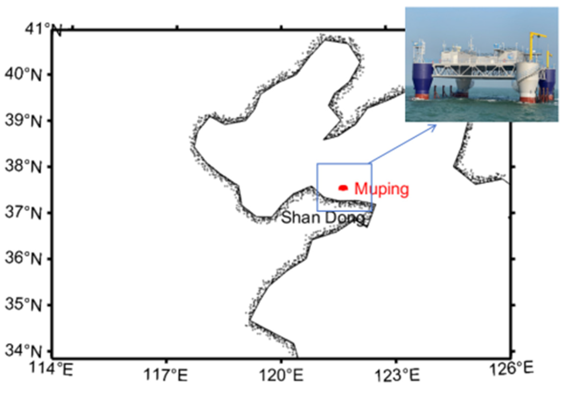
The Mu Ping site (37.681N, 121.700E) is located in the coastal area approximately 20 km north of the coastline in the Mu Ping district of Yantai City, Shandong Province, as shown in Figure 1. Situated near the junction of the Bohai Sea and Yellow Sea, this site experiences a dual influence from both the ocean and the mainland due to its proximity to the coastline. The station employs the CE318 Sun Photometer, a water color version manufactured by the French company CIMEL Electronics. It comprises 11 observation channels at wavelengths of 400 nm, 412 nm, 442 nm, 490 nm, 510 nm, 560 nm, 620 nm, 665 nm, 779 nm, 865 nm, and 1020 nm. In atmospheric aerosol research, the wavelengths of 442 nm, 665 nm, 865 nm, and 1020 nm are commonly used [26]. The instrument primarily measures solar radiance, allowing for the estimation of atmospheric aerosol characteristics and other components.
The CE318 multi-band sun photometer, using the PhotoGetData (v2.18.5) software, can transmit the measured data through the RS232 serial port to a computer and save it, generating binary storage files (K8 files). Each K8 file, after conversion into ASCII format, typically includes multiple file types with different suffixes. Among them, the NSU file represents data for direct solar radiation measurements, primarily used for calculating aerosol optical thickness and other parameters. The ALL and ALR files, respectively, denote data for zenith angle scans in the sky and left–right scans along the azimuth circle, mainly used for inverting sky radiance parameters. The sun photometer data at this site are sourced from the National Satellite Ocean Application Center.
2.1.2. Remote Sensing Images
MODIS is equipped with 36 spectral bands, among which 16 are primarily suitable for water color research, including 10 visible bands, 3 Near-Infrared bands, and 3 Short-Wave Infrared bands. The high temporal resolution of MODIS sensor provides significant advantages for studying rapidly changing water color in time dynamics, making it one of the widely used image data globally. For turbid coastal waters, MODIS’s Short-Wave Infrared bands can effectively serve atmospheric correction work. MODIS sensor provides various level data products, including L0, L1A, L1B, L2, and L3. L0 data are the raw data received by the sensor without processing, which is only used in a few specific applications. L1A data are reconstructed from L0 data and supplemented with auxiliary information (including radiometric and geometric calibration coefficients, as well as geolocation parameters). L1B data are radiometrically calibrated L1A data. L2 data are the geophysical products developed by combining L1B data with auxiliary data through processes such as atmospheric correction and parameter inversion. L3 data are raster data obtained by uniform mosaicking and projecting L2 products over a certain geographic grid within a certain time period. In this article, MODIS Aqua L1A data are used as the source of remote sensing image data to validate the atmospheric correction results obtained from aerosol models. The data were downloaded from NASA (https://oceancolor.gsfc.nasa.gov/, accessed on 1 October 2023).
2.1.3. Rrs Validation Data
This study utilizes on-site measurements of spectra from the Mu Ping station, established by the National Satellite Ocean Application Center on the northern coast of the Shandong Peninsula. The dataset includes measurements collected from the year 2020 to the present. When conducting measurements, the method used was that recommended by NASA for obtaining above-water remote sensing reflectance () data [27], which were estimated as
where is the upward radiance, denotes skylight radiance, represents the radiance emitted from a standard reference plaque, all of which were directly measured using a spectrometer. represents the reflectance (approximately 10%) of a standard reference plaque provided by the producer, and signifies the Fresnel reflection off the water surface, assumed to be 0.022 for a flat water surface.
2.2. Methods
2.2.1. Construction of Aerosol Models
The raw data used for the inversion of aerosol microphysical properties comes from the Mu Ping station’s CE318 Water Color Sun/Sky Photometer. The microphysical characteristics of aerosols, including particle size distribution and complex refractive index, can be inferred from spectral sky radiance measurements conducted at 442, 665, 865, and 1020 nm, obtained at the almucantar plane, along with solar direct irradiance measurements at corresponding wavelengths [26]. The selected four bands exhibit no significant gas absorption and demonstrate high sensitivity to the typical sizes of major aerosols [28]. Before the inversion of microphysical properties, it is necessary to select data that meet certain criteria. First, the observed sky radiance data from both left and right azimuth scans (clockwise and counterclockwise) should differ by no more than 20%. The average of the left and right azimuth scan data is then taken as the sky radiance data for that specific time point. Second, under the condition of symmetric azimuth angles for left and right sky scattering radiance, the scattering radiance data used for inversion should have a symmetrical azimuthal angle count greater than 21, within the range of 3.5° to 160° [29]. Third, the selected data should have a solar zenith angle greater than 50°. The data generated under this criterion is similar to the AERONET website’s version 2.0 data [29,30]. The sky radiance data were convolved using a square filter with a width of 10 nm centered at the effective wavelengths of the photometer. The standard extraterrestrial spectrum irradiance (https://oceancolor.gsfc.nasa.gov/docs/rsr/f0.txt, accessed on 1 October 2023) was used to normalize the resulting spectra [31].
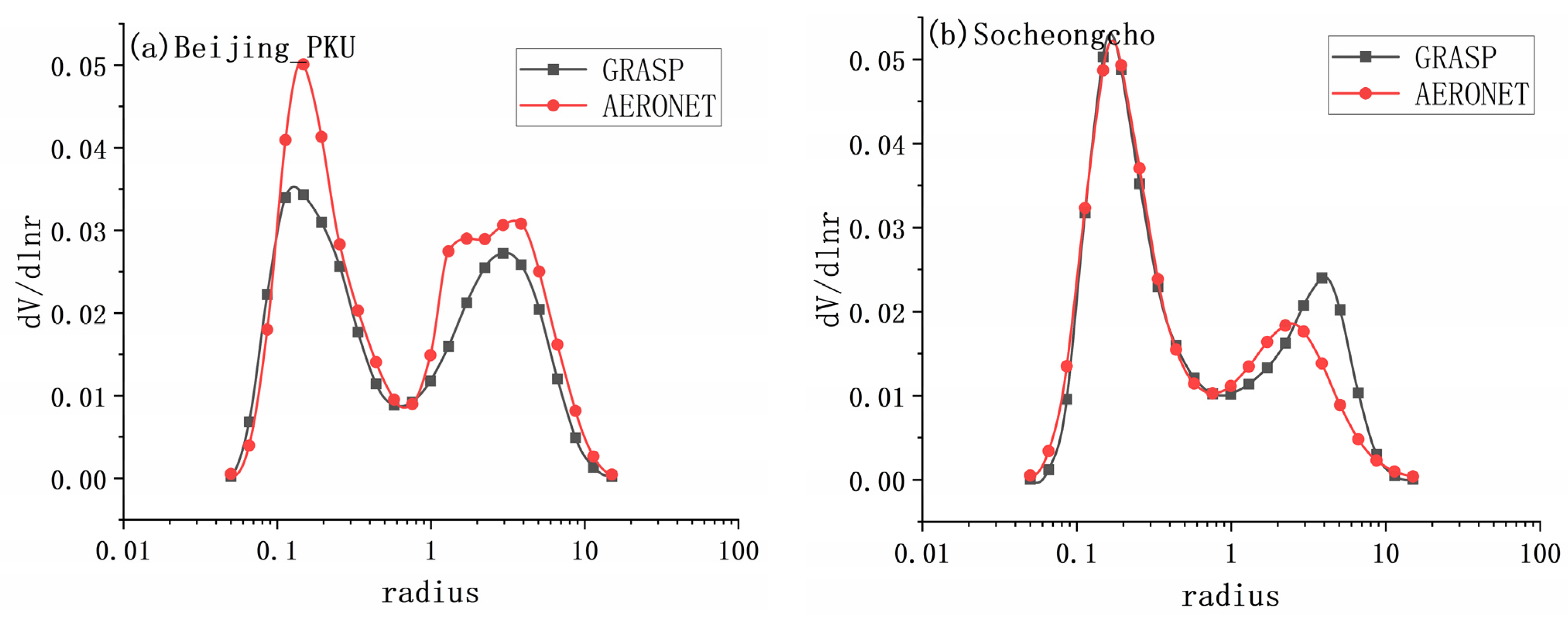
The Generalized Retrieval of Aerosol and Surface Properties (GRASP) code, developed by Dubovik et al., is an open-source algorithm designed for retrieving properties of aerosols [30,32,33]. GRASP comprises two main modules: numerical inversion and forward modeling. The numerical inversion module employs statistical optimization techniques to fit observational data, while the forward model accurately simulates various atmospheric remote sensing observations [34]. Therefore, this versatility allows GRASP to be applied across passive and active satellites, as well as ground-based atmospheric observations, and it is particularly suited for synergistic retrievals when inverting different observations simultaneously [35]. The algorithm accepts diverse input data, such as satellite images, polar nephelometer measurements, sun/sky photometer data, sky camera images, and lidar data. The precise inversion of various combinations of these input data is accomplished through the use of a multi-term least squares method (LSM) [36]. This fitting algorithm can undergo statistical optimization, allowing for flexible inversions based on different observations [37]. In this study, ground-based observations from a single sun photometer were utilized for the inversion of aerosol properties. The retrieved column-integrated aerosol volume size distributions (VSDs) are adjusted using 22 logarithmically equidistant triangle bins ranging from 0.05 to 15 µm in radius [38]. While some studies suggest approximating VSDs with bimodal log-normal distributions to reduce the information required by the binned VSDs, a problem arises when the retrieved VSDs deviate from perfect log-normality, leading to asymmetrical or trimodal shapes. In such cases, the strategy based on simplified bimodal VSDs may not yield accurate retrievals, hence the preference for the former approach despite its more complex calculations. To further validate the algorithm’s reliability and ensure the accuracy of the results, we selected raw data from the AERONET Beijing_PKU and Socheongcho sites as input for the GRASP algorithm [39]. We inverted the aerosol particle size distribution for the respective regions of these two sites. The Beijing_PKU site is located on land, and the data selected are from 1 January 2019, at 01:21:13 UTC. The Socheongcho site is situated in the ocean, and the data retrieved are from 3 January 2020, at 03:48:35 UTC. These two sites represent different underlying surface types. The obtained results are shown in Figure 2.
For the Beijing_PKU site, it can be observed that the trend of aerosol size distribution obtained by the GRASP algorithm is generally consistent with the AERONET results. However, a notable difference is that the AERONET results exhibit higher peaks at the coarse and fine modal particles compared to the GRASP results. For the Socheongcho site, the consistency between GRASP and AERONET results is nearly perfect, with only minor differences observed at the peak of coarse-mode particles. This suggests that the GRASP algorithm is capable of accurately retrieving aerosol characteristics in the respective regions.
In open ocean regions, the distribution of aerosol particles in the air above the sea surface is relatively stable, with less influence from external factors, and the composition and concentration of aerosols change minimally with the seasons [22]. However, in coastal areas, due to proximity to land, the composition of aerosols in the atmosphere above undergoes rapid changes in both time and space, influenced significantly by human activities and natural factors on land, and is subject to larger variations due to terrestrial influences [40].
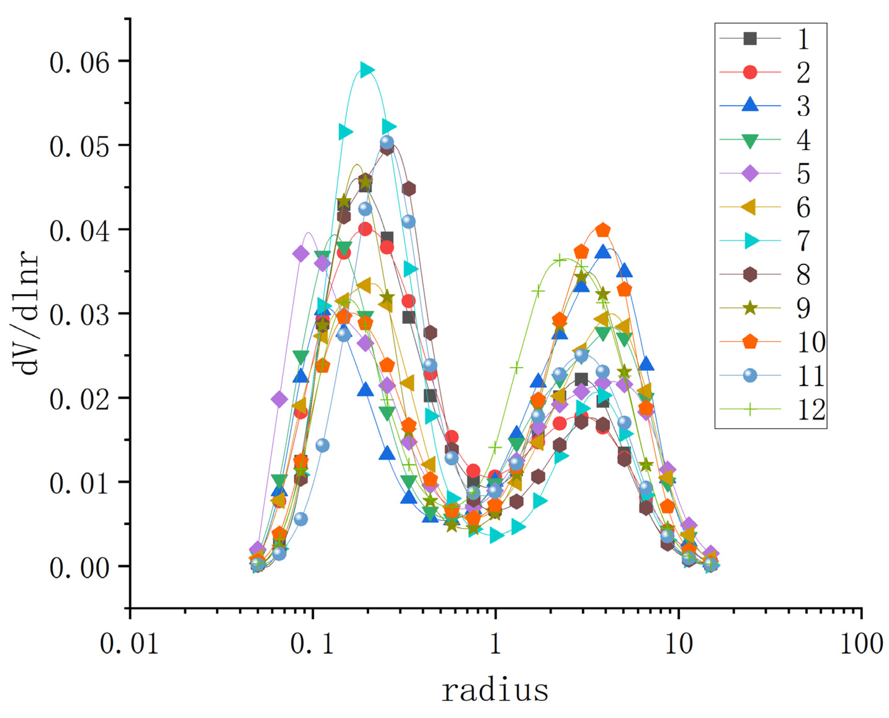
The AF10 model, currently adopted as the globally standardized aerosol model by NASA, incorporates relative humidity as a key parameter to adapt various regional aerosol models. However, aerosol particles originating from terrestrial sources, including continental, biomass burning, and dust sources, demonstrated limited sensitivity to variations in relative humidity, particularly under conditions where the relative humidity is below 70% [41,42]. Kinne’s study of aerosol characteristics on the monthly average time scale found that large monthly differences were rare [43]. Sang Woo studied the optical properties of columnar aerosols in East Asia and found that their changes had seasonal and monthly characteristics [44]. Through studying the global aerosol particle size distribution and complex refractive index parameters, Zhao Dan found that these parameters changed slightly in the same month in different years and were relatively stable [1]. Therefore, for more accurate construction of regional aerosol models, this study builds aerosol models for the region based on monthly aerosol data. Selecting the sun photometer data from the Mu Ping station between 2020 and 2022, which underwent quality control, the GRASP algorithm is employed to invert aerosol microphysical and optical properties. Results with inversion fitting errors of less than 5% are considered valid. Valid results are then statistically analyzed, and monthly averages are calculated to construct monthly aerosol models. The microphysical properties of aerosols, including particle size distribution and complex refractive index, along with optical properties such as extinction coefficient, Ångström exponent (α), single scattering albedo (SSA), and aerosol phase function, can be simulated using a radiative transfer model predicated on these pivotal microphysical attributes [45].
The aerosol size distribution function describes how particles of different diameters are distributed within a given volume. Typically, this function is modeled as the combination of two log-normal distributions: one for fine particles and the other for coarse particles. This combined distribution is commonly known as a bimodal log-normal distribution. Mathematically, it can be represented as follows:
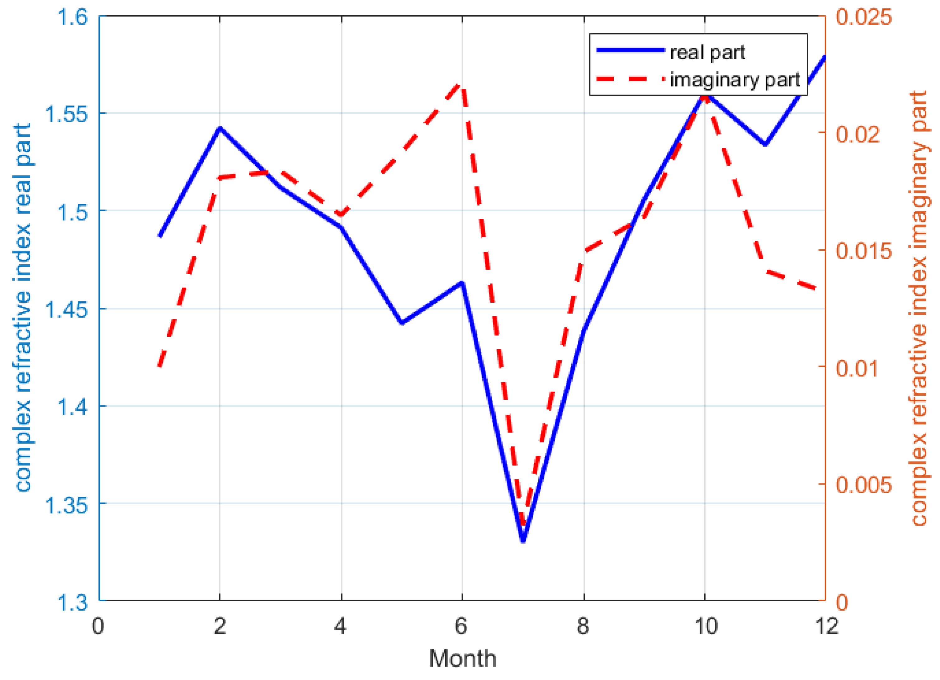
where V denotes the volume concentration of the particles, r represents the mean volume radius of the particles, and represent coarse mode particles and fine mode particles, respectively. and represent the mean volume radius of the fine and coarse mode particles, respectively. and signify the standard deviation of the fine mode and coarse mode particle size within a model. Figure 3 shows the monthly average particle size distribution at the Mu Ping station for months 1 to 12 [43]. The complex refractive index comprises the real part () and the imaginary part (), which vary depending on the chemical composition of the aerosol; and govern the scattering and absorption of aerosols by incident light, respectively [46,47]. Figure 4 illustrates the distribution of the real and imaginary components of the complex refractive index at 442 nm across months 1 to 12. In July, there is only one valid data point, and thus, it lacks monthly representativeness. By inputting the aforementioned particle size distribution and complex refractive index into the 6S radiative transfer model, the optical properties of aerosols can be simulated [48].
2.2.2. Construction of the Lookup Table for the New Aerosol Model
These tables contain parameters identical to those used in the AF10 model. Additionally, two sets of coefficients were computed. The first set represents the correlation between single-scattering albedo and multiple-scattering albedo. The second set of coefficients relates to the relationship between diffuse transmittance from the sun to Earth’s surface, diffuse transmittance from the surface to the satellite, and aerosol optical thickness.
In the case where geometric conditions and aerosol optical thickness (AOD) are known, the relationship between aerosol single-scattering reflectance () and aerosol multiple-scattering reflectance () can be expressed as
where is aerosol single scattering albedo, is aerosol optical depth, and are solar zenith angle and view zenith angle, respectively, is relative azimuth angle, is the aerosol scattering phase function for a scattering angle, , is the Fresnel reflectance of the interface for an incident angle .
Whereas the multiple-scattering reflectance is obtained through simulations using the 6S radiative transfer model [48], the single-scattering reflectance is calculated using Equations (4) and (5) [49].
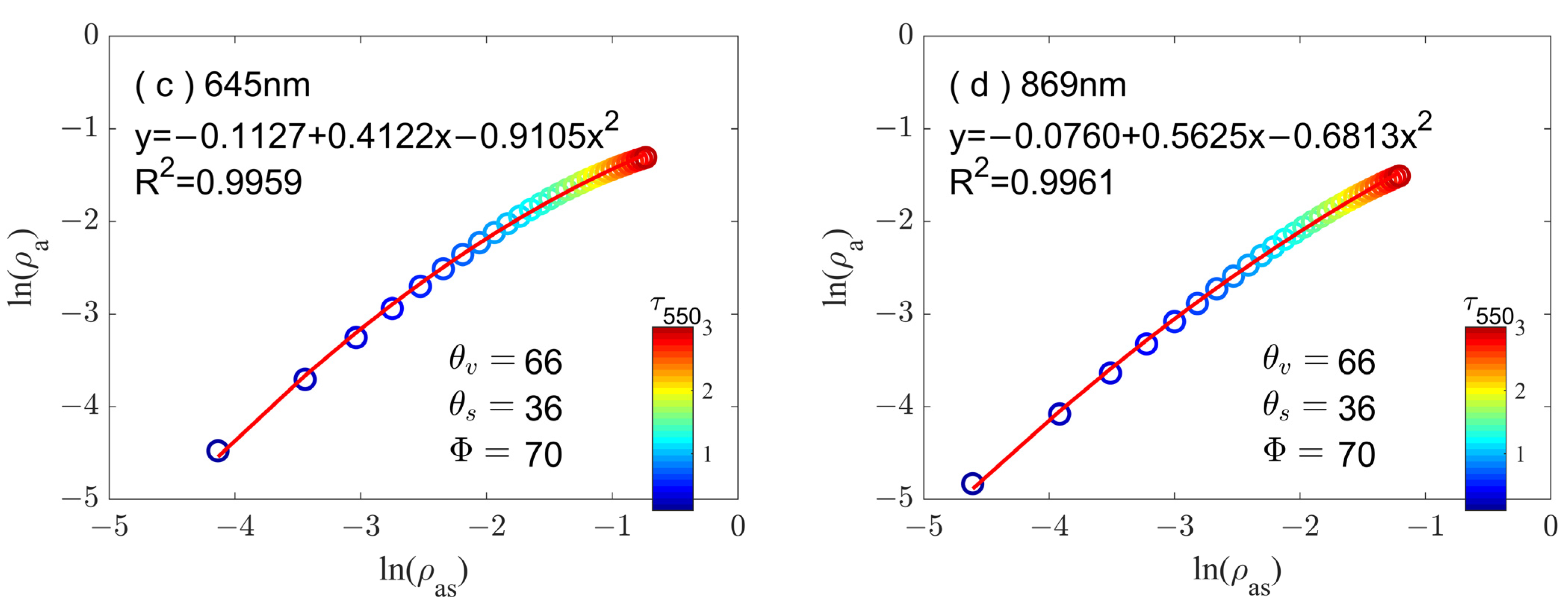
By employing the method of least squares fitting regression to solve for the coefficients a, b, and c, the relationship between and under specific geometric conditions (°, °, °) for the aerosol model at the Mu Ping station in June is depicted in Figure 5. The regression coefficients in the regression equation correspond to the a, b, and c in Equation (3).
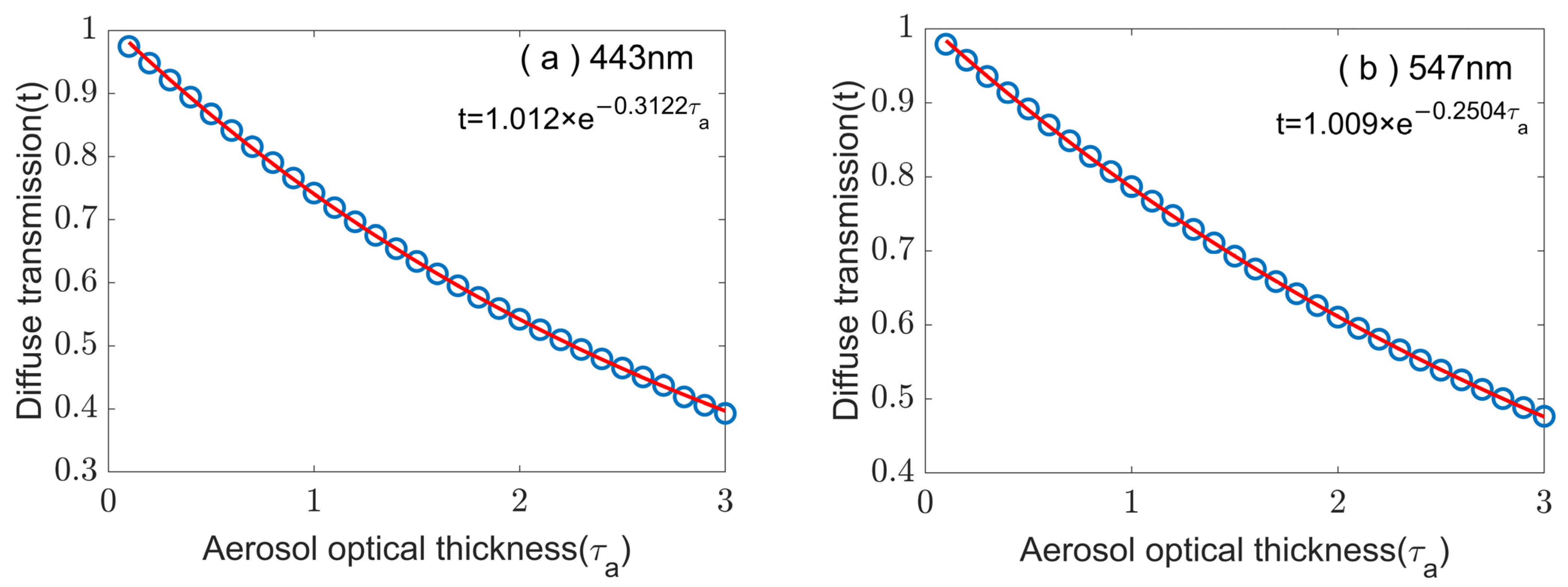
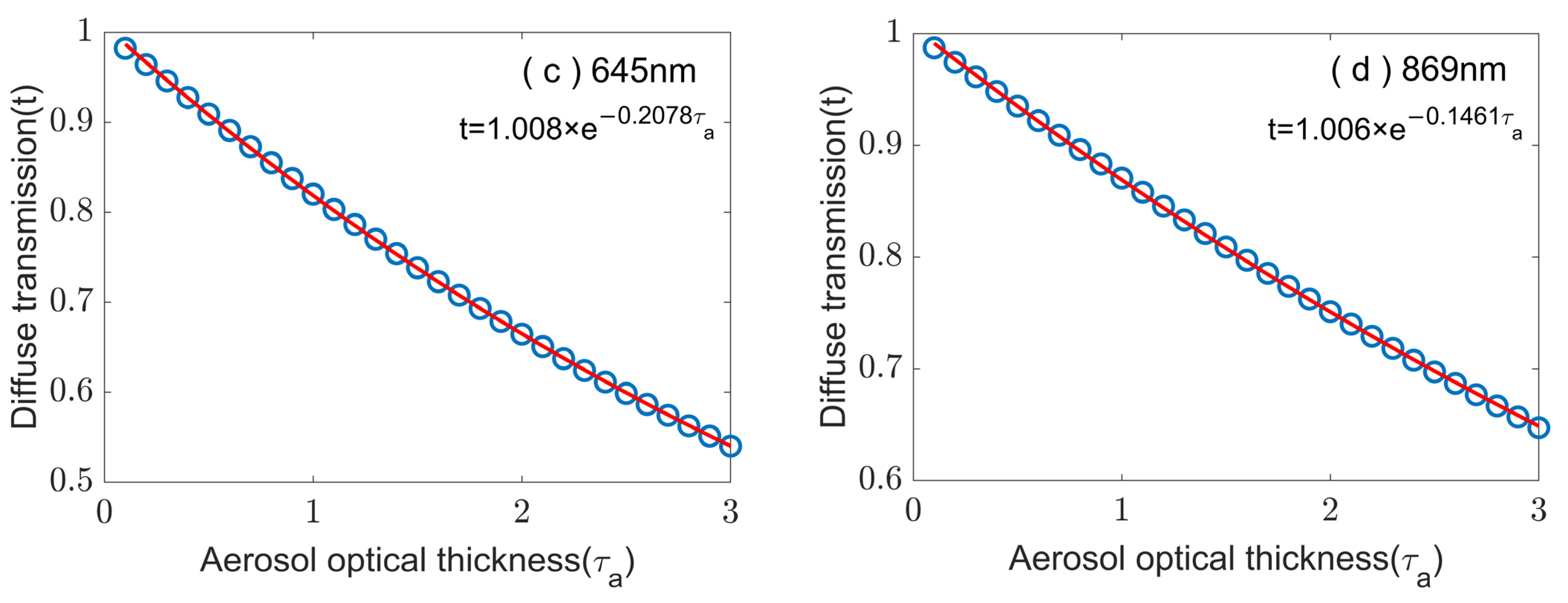
The relationship between diffuse transmittance t ( or ) and aerosol optical depth () can be expressed as
Whereas the diffuse transmittance t is obtained through simulations using the 6S radiative transfer model under specific geometric parameters and AOD conditions, the coefficients (A and B) can be obtained through the least squares fitting method. Figure 6 depicts the relationship between diffuse transmittance and aerosol optical depth when the solar zenith angle is 36 degrees, and the coefficients of the fitting equation correspond to the A and B in Equation (7).
For each lookup table (LUT) associated with the aerosol model for each month, we integrated diverse combinations of aerosol multiple-scattering and diffuse transmittance coefficients correlated with aerosol optical depth (AOD) values and satellite/solar geometric parameters. In particular, the AOD varied from 0 to 3 (with an increment of 0.1), while the solar/sensor zenith angles ( and ) ranged from 0 to 78 degrees (with an increment of 6 degrees), and their relative azimuthal angles () ranged from 0 to 180 degrees (with an increment of 10 degrees). Conversely, NASA’s LUT employed only 8 AOD values within a significantly narrower range [4]. The format and content of the aerosol lookup table are shown in Table 1.
2.2.3. Atmospheric Correction
The radiative signals observed by satellite sensors include signals from both water bodies and the atmosphere [21,50]. To achieve more accurate retrieval of water color elements, it is essential to separate the water color signal from the atmospheric signal [51,52,53]. The process of removing the atmospheric signal is known as atmospheric correction [54,55].
The goal of atmospheric correction is to establish specific models that remove atmospheric path and surface influences from the Top of Atmosphere (TOA) signals. The primary difficulty involves accurately assessing the impact of aerosols, a major source of uncertainty in atmospheric correction, on atmospheric path radiance. This contribution varies considerably and must be estimated based on observations [56]. Water exhibits strong absorption in the Near-Infrared to Short-Wave Infrared (NIR-SWIR) range, providing a basis for separating atmospheric and ocean signals [57,58]. Initially, for open ocean regions, SeaWiFS and MODIS atmospheric correction was conducted using two Near-Infrared (NIR) bands under the assumption that the marine influence in these NIR bands could be considered negligible [50]. However, coastal regions, influenced by factors such as land–sea dynamics, often have turbid waters. In these areas, the radiance observed in the Near-Infrared (NIR) bands can be significant. This can pose challenges for iterative methods that rely solely on NIR, leading to underestimation or even negative values for water-leaving radiance. To tackle this issue, Wang et al. [59] proposed an atmospheric correction algorithm for MODIS that incorporates both Near-Infrared and Short-Wave Infrared bands. The key aspect of this algorithm involves introducing a turbidity index based on MODIS measurements in the Near-Infrared (748 nm) and Short-Wave Infrared bands (1240 nm, 2130 nm), as described in Equation (7). When the turbidity index meets certain conditions , the iterative method using Near-Infrared bands (748 nm, 869 nm) is applied; otherwise, the iterative method using Short-Wave Infrared bands (1240 nm, 2130 nm) is utilized [59,60].
where represents the reflectance of the top atmosphere observed by satellites after gas absorption correction, and denotes the reflectance contributed by the molecules, also known as Rayleigh scattering.
3. Results
To further validate the efficacy of our new aerosol model in improving atmospheric correction, we applied the previously described NIR-SWIR atmospheric correction algorithm. This algorithm, recommended jointly by NASA for turbid water bodies, was validated utilizing datasets on a global and regional scale. The monthly Look-Up Tables (LUTs) developed for the study sites in this research were substituted for the standard LUTs in the SeaDAS (v8.3) software. During the atmospheric correction process for a specific pixel, the aerosol LUT is selected based on the location of the target pixel and the month of data collection. Subsequently, this LUT is utilized to estimate the aerosol scattering component of the signal [1].
This research utilized the same version of SeaDAS (v8.3) for the removal of gas absorption and Rayleigh scattering to assess the improvements of the new aerosol model on remote sensing reflectance () products. We established specific criteria for selecting corresponding satellite and in situ observational data. Initially, the time interval between satellite observations and ground-based measurements was limited to 30 min. While NASA’s standard allows a 3 h time difference in open ocean regions, our stricter criterion was necessary due to the higher variability and influence of continental factors in coastal areas. Pixels identified as being affected by cloud or ice contamination, having high sensor view zenith, high solar zenith, and stray light contamination were deemed invalid. Instead of using NASA’s default Rayleigh-corrected reflectance for cloud-masked reflectance, we opted for an alternative approach [1]. This decision was made due to concerns that NASA’s default threshold might incorrectly identify turbid water or thick aerosols, which are common in coastal waters. Similar methodologies were adopted in previous research studies [61,62].
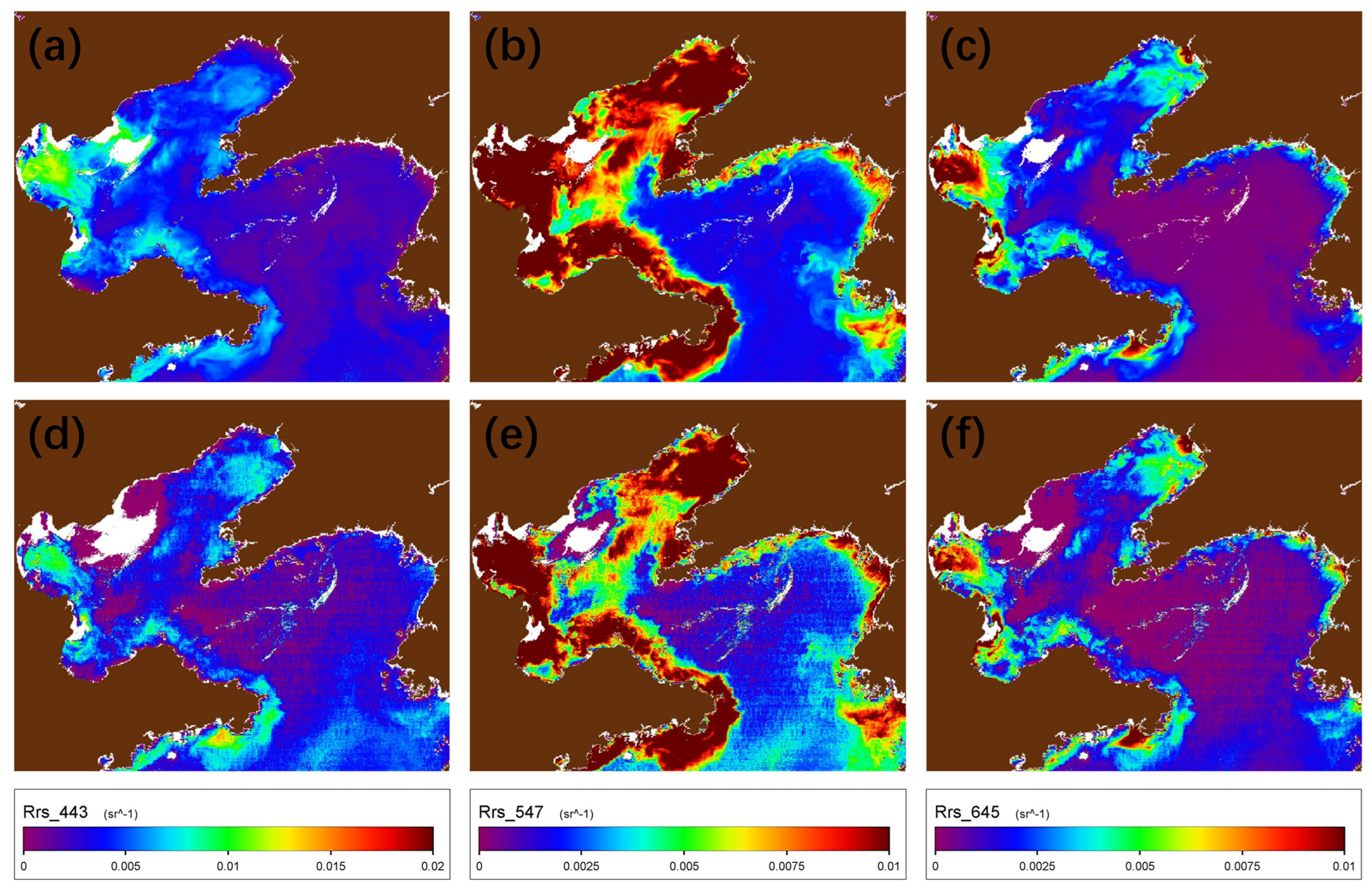
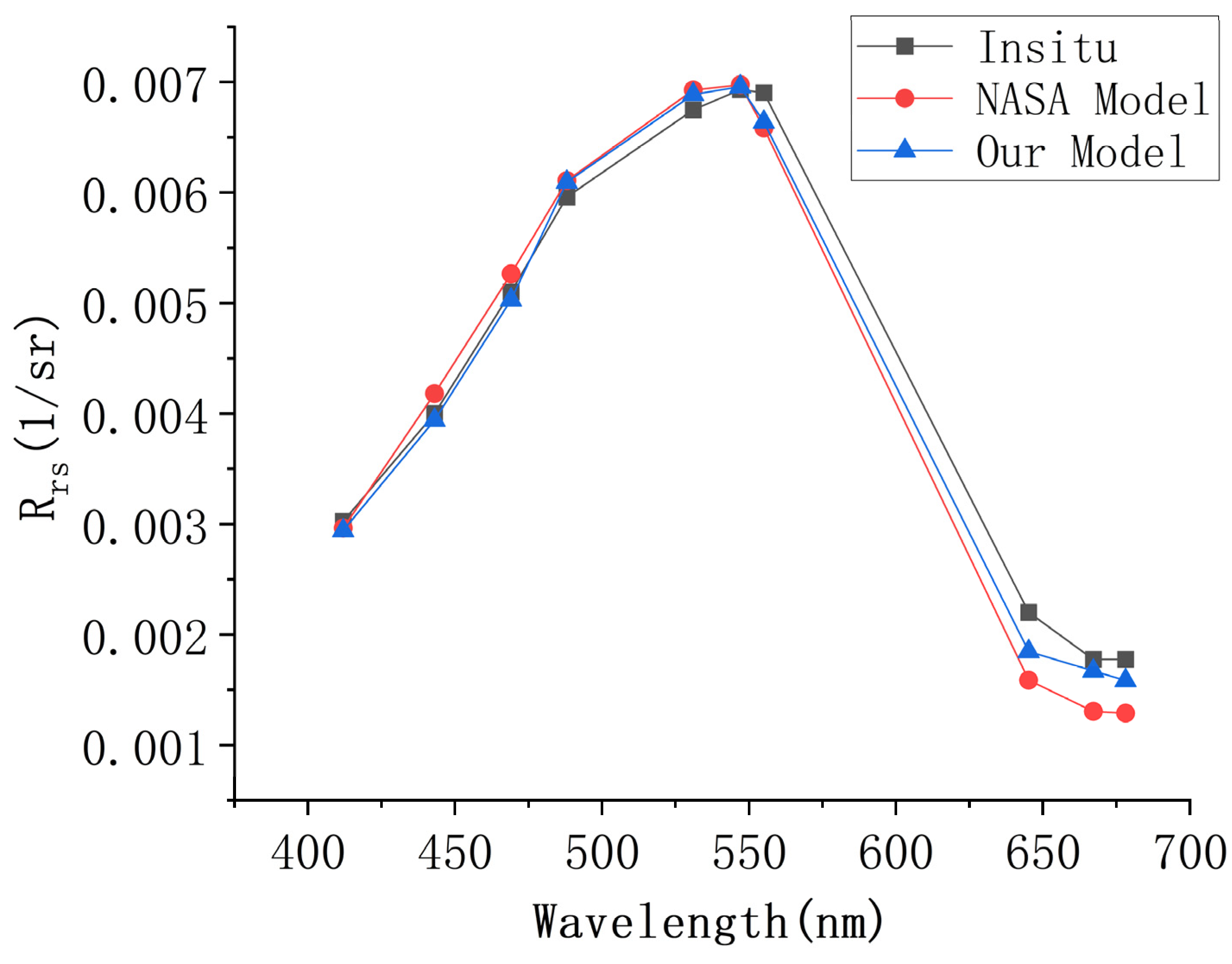
Figure 7 shows the remote sensing reflectance () obtained from the aerosol model developed in this study and the AF10 aerosol model processed through the NIR-SWIR algorithm. It can be observed that the distribution from the two models is generally consistent, with subtle differences in specific values. In certain regions, the aerosol model established in this article yields slightly higher than the NASA standard model. This means that the aerosol signals assessed by standard aerosol models in these regions may be higher than those in the aerosol models presented in this paper. This is due to the fact that standard aerosol models are constructed using only a small number of observations from ocean sites, especially in coastal areas. This results in the overestimation of aerosol signals in turbid water, while the measured aerosol data in this paper can better characterize the aerosol characteristics of the study area, and the aerosol signals obtained are more accurate. Figure 8 presents a further comparison between satellite-retrieved and ground-based measured spectra. For this collection of spectra, in strict adherence to the previously defined criteria, the time gap between satellite imagery and ground measurements does not exceed 30 min. It can be seen that when we use the new aerosol model, the results calculated by the NIR-SWIR algorithm are closer to the measured values.
4. Discussion
We use several accuracy assessment metrics to evaluate the results of the aerosol model, encompassing the regression slope, coefficient of determination (), root mean squared difference (RMSD), unbiased percentage difference (UPD), and mean absolute error (MAE).
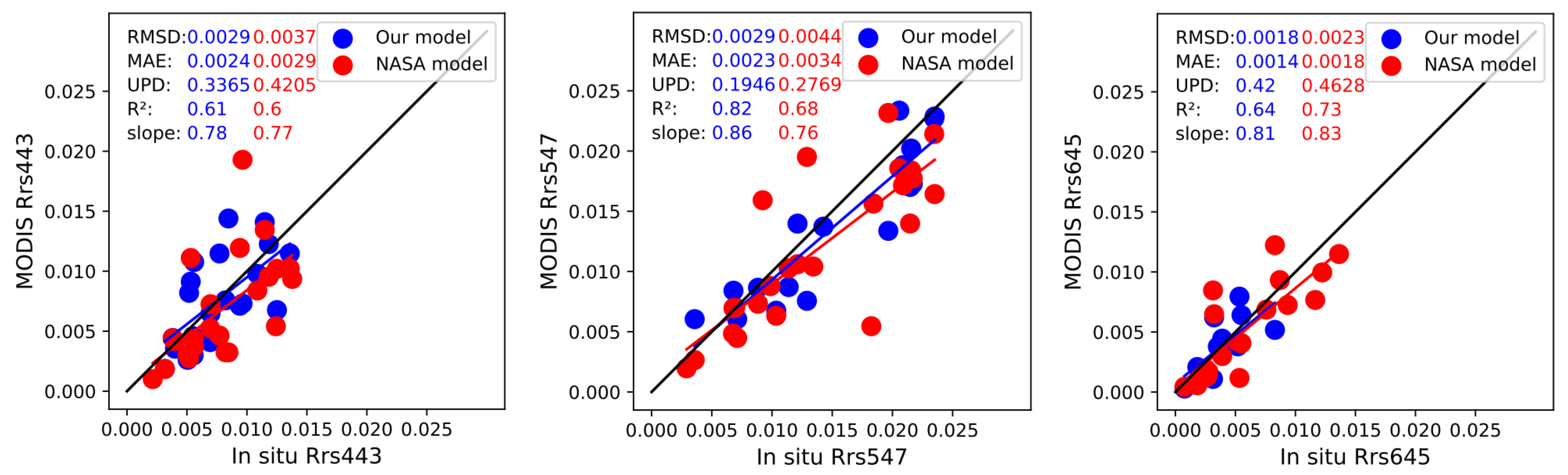
Figure 9 displays the satellite data alongside corresponding measurements for three visible bands (i.e., 443, 547, and 645 nm), and the satellite product is also calculated using the NIR-SWIR algorithm. The red points represent the results of NASA’s standard aerosol model, while the blue points represent the results of the new aerosol model proposed in this study.
From the results, it is clear that for the RMSD, MAE, and UPD accuracy evaluation indicators, the results of the new model are significantly better than NASA’s standard model. For and slope, except for slightly lower values at 645 nm, the new model’s results at 443 nm and 547 nm are also better than the standard model. Table 2 lists the accuracy assessment statistics for MODIS’s nine bands. Overall, the performance of the new aerosol model is better than the standard aerosol model, especially at 547 nm. It is important to highlight that the underestimation observed in the blue light band with the new model, relative to the standard model, was mitigated, which is likely attributed to a more accurate representation of absorbing aerosols [1]. It is notable that the slopes observed in these bands are all less than 1, possibly indicating the overcorrection of remote sensing reflectance () in turbid water. Please note that the study initially matched 24 satellite situ points. However, minor discrepancies in the number of data points across different models or bands may arise from saturation or negative values in MODIS bands or from the atmospheric correction process.
5. Conclusions
Coastal regions, characterized by complex water compositions, introduce significant uncertainties in remote sensing reflectance () obtained through atmospheric correction. NASA’s aerosol models are primarily developed for open ocean conditions, leading to substantial variability in coastal areas, mainly due to the inaccurate characterization of absorbing aerosols in the aerosol correction process. In this study, aerosol observation data from the Mu Ping station in the Yellow and Bohai Seas were utilized to characterize aerosol properties in the region. Aerosol properties, such as single scattering albedo (SSA) and Ångström exponent, exhibited noticeable spatial gradients and seasonal dynamics. The monthly aerosol model, based on these aerosol characteristics by taking their monthly averages, can more effectively characterize the scattering and absorption properties of aerosols in the region, facilitating the precise removal of aerosol signals from the sensor-received signals. By incorporating this aerosol model and the standard aerosol model into the NIR-SWIR algorithm for atmospheric correction, the atmospheric correction results for both models in the region are obtained. These results are then matched and validated against measured data. From the precision evaluation metrics, including RMSD, MAE, and UPD, it can be observed that the new aerosol model outperforms the standard aerosol model across the nine visible light bands of MODIS, leading to an improvement in the accuracy of atmospheric correction.
While we only applied this aerosol model to MODIS satellite imagery in this study, it can seamlessly be adapted for use with other satellite imagery. This adaptation requires constructing aerosol model lookup tables that align with the specific wavelength bands of the other satellites. This opens up the possibility of generating additional remote sensing reflectance () products for coastal regions, facilitating the improved retrieval of water color-related parameters.
Certainly, there is substantial room for improvement in the current aerosol model. The model’s construction was based on observational data from the Mu Ping station spanning 2020 to 2022, which is relatively limited. As time progresses, the Mu Ping station will provide more observational data, enabling the aerosol model to better capture the seasonal dynamic changes in aerosol characteristics. This will facilitate more effective atmospheric correction efforts. Depending on requirements, aerosol models can be constructed with smaller time intervals. Presently, the Huangdonghai offshore observation platform has deployed two observation stations, Mu Ping and Dongtou. In the future, more aerosol observation stations will be established in China’s offshore areas, achieving comprehensive coverage of aerosol characteristic observations in the Chinese near seas. This holds extraordinary significance for obtaining precise products in China’s nearshore regions.
Author Contributions
Conceptualization, K.S.; methodology, K.S. and J.L.; validation, K.S.; investigation, K.S.; resources, K.S.; data curation, K.S.; writing—original draft, K.S.; writing—review and editing, C.M., Q.S. and D.Z.; visualization, K.S.; supervision, C.M., Q.S. and D.Z.; project administration, Q.S.; funding acquisition, Q.S.; All authors have read and agreed to the published version of the manuscript.
Funding
This research was funded by the National Natural Science Foundation of China under grant number 42176183.
Data Availability Statement
Dataset available upon request from the authors.
Acknowledgments
We acknowledge the data support from the National Satellite Ocean Application Service (http://www.nsoas.org.cn/) and NASA GSFC (https://oceancolor.gsfc.nasa.gov/). We thank the reviewers for their valuable feedback on the paper.
Conflicts of Interest
The authors declare no conflicts of interest.
References
- Zhao, D.; Feng, L.; He, X. Global gridded aerosol models established for atmospheric correction over inland and nearshore coastal waters. J. Geophys. Res. Atmos 2023, 128, e2023JD038815. [Google Scholar] [CrossRef]
- Wei, J.; Lee, Z.; Shang, S. A system to measure the data quality of spectral remote-sensing reflectance of aquatic environments. J. Geophys. Res. Oceans 2016, 121, 8189–8207. [Google Scholar] [CrossRef]
- Mukai, S.; Sano, I.; Toigo, A. Removal of scattered light in the Earth atmosphere. Earth Planets Space 1998, 50, 595–601. [Google Scholar] [CrossRef]
- Gordon, H.R. Atmospheric correction of ocean color imagery in the Earth Observing System era. J. Geophys. Res. Atmos 1997, 102, 17081–17106. [Google Scholar] [CrossRef]
- Mobley, C.D.; Werdell, J.; Franz, B.; Ahmad, Z.; Bailey, S. Atmospheric Correction for Satellite Ocean Color Radiometry; Goddard Space Flight Center: Washington, DC, USA, 2016. [Google Scholar]
- Shi, C.; Nakajima, T. Simultaneous determination of aerosol optical thickness and water-leaving radiance from multispectral measurements in coastal waters. Atmos. Chem. Phys. 2018, 18, 3865–3884. [Google Scholar] [CrossRef]
- Kompalli, S.K.; Suresh Babu, S.; Krishna Moorthy, K.; Gogoi, M.M.; Nair, V.S.; Chaubey, J.P. The formation and growth of ultrafine particles in two contrasting environments: A case study. Ann. Geophys. 2014, 32, 817–830. [Google Scholar] [CrossRef]
- Sayer, A.; Hsu, N.; Bettenhausen, C.; Ahmad, Z.; Holben, B.; Smirnov, A.; Thomas, G.; Zhang, J. SeaWiFS Ocean Aerosol Retrieval (SOAR): Algorithm, validation, and comparison with other data sets. J. Geophys. Res. Atmos 2012, 117, D3. [Google Scholar] [CrossRef]
- Bassani, C.; Manzo, C.; Braga, F.; Bresciani, M.; Giardino, C.; Alberotanza, L. The impact of the microphysical properties of aerosol on the atmospheric correction of hyperspectral data in coastal waters. Atmos. Meas. Tech. 2015, 8, 1593–1604. [Google Scholar] [CrossRef]
- Gordon, H.R.; Du, T.; Zhang, T. Remote sensing of ocean color and aerosol properties: Resolving the issue of aerosol absorption. Appl. Opt. 1997, 36, 8670–8684. [Google Scholar] [CrossRef]
- Omar, A.H.; Won, J.G.; Winker, D.M.; Yoon, S.C.; Dubovik, O.; McCormick, M.P. Development of global aerosol models using cluster analysis of Aerosol Robotic Network (AERONET) measurements. J. Geophys. Res. Atmos 2005, 110, D10S14. [Google Scholar] [CrossRef]
- Shettle, E.P.; Fenn, R.W. Models for the Aerosols of The Lower Atmosphere and the Effects of Humidity Variations on Their Optical Properties; Optical Physics Division, Air Force Geophysics Laboratory: Birmingham, AL, USA, 1979. [Google Scholar]
- Tanré, D.; Kaufman, Y.; Herman, M.; Mattoo, S. Remote sensing of aerosol properties over oceans using the MODIS/EOS spectral radiances. J. Geophys. Res. Atmos 1997, 102, 16971–16988. [Google Scholar] [CrossRef]
- Logan, T.; Xi, B.; Dong, X.; Li, Z.; Cribb, M. Classification and investigation of Asian aerosol absorptive properties. Atmos. Chem. Phys. 2013, 13, 2253–2265. [Google Scholar] [CrossRef]
- von Bismarck-Osten, C.; Weber, S. A uniform classification of aerosol signature size distributions based on regression-guided and observational cluster analysis. Atmos. Environ. 2014, 89, 346–357. [Google Scholar] [CrossRef]
- Davies, C. Size distribution of atmospheric particles. J. Aerosol Sci. 1974, 5, 293–300. [Google Scholar] [CrossRef]
- Chomko, R.M.; Gordon, H.R. Atmospheric correction of ocean color imagery: Use of the Junge power-law aerosol size distribution with variable refractive index to handle aerosol absorption. Appl. Opt. 1998, 37, 5560–5572. [Google Scholar] [CrossRef] [PubMed]
- Deirmendjian, D. Scattering and polarization properties of water clouds and hazes in the visible and infrared. Appl. Opt. 1964, 3, 187–196. [Google Scholar] [CrossRef]
- Junge, C.E. Our knowledge of the physico-chemistry of aerosols in the undisturbed marine environment. J. Geophys. Res. 1972, 77, 5183–5200. [Google Scholar] [CrossRef]
- Yu, Q.-R.; Zhang, F.; Li, J.; Zhang, J. Analysis of sea-salt aerosol size distributions in radiative transfer. J. Aerosol Sci. 2019, 129, 71–86. [Google Scholar] [CrossRef]
- Gordon, H.R.; Wang, M. Retrieval of water-leaving radiance and aerosol optical thickness over the oceans with SeaWiFS: A preliminary algorithm. Appl. Opt. 1994, 33, 443–452. [Google Scholar] [CrossRef]
- Ahmad, Z.; Franz, B.A.; McClain, C.R.; Kwiatkowska, E.J.; Werdell, J.; Shettle, E.P.; Holben, B.N. New aerosol models for the retrieval of aerosol optical thickness and normalized water-leaving radiances from the SeaWiFS and MODIS sensors over coastal regions and open oceans. Appl. Opt. 2010, 49, 5545–5560. [Google Scholar] [CrossRef]
- Frouin, R.; Deschamps, P.-Y.; Gross-Colzy, L.; Murakami, H.; Nakajima, T.Y. Retrieval of chlorophyll-a concentration via linear combination of ADEOS-II Global Imager data. J. Oceanogr 2006, 62, 331–337. [Google Scholar] [CrossRef]
- Bru, D.; Lubac, B.; Normandin, C.; Robinet, A.; Leconte, M.; Hagolle, O.; Martiny, N.; Jamet, C. Atmospheric correction of multi-spectral littoral images using a PHOTONS/AERONET-based regional aerosol model. Remote Sens. 2017, 9, 814. [Google Scholar] [CrossRef]
- Montes, M.; Pahlevan, N.; Giles, D.M.; Roger, J.-C.; Zhai, P.-w.; Smith, B.; Levy, R.; Werdell, P.J.; Smirnov, A. Augmenting heritage ocean-color aerosol models for enhanced remote sensing of inland and nearshore coastal waters. Front. Remote Sens. 2022, 3, 860816. [Google Scholar] [CrossRef]
- Molero, F.; Pujadas, M.; Artíñano, B.J.R.S. Study of the Effect of Aerosol Vertical Profile on Microphysical Properties Using GRASP Code with Sun/Sky Photometer and Multiwavelength Lidar Measurements. Remote Sens. 2020, 12, 4072. [Google Scholar] [CrossRef]
- Mobley, C.D.; Zhang, H.; Voss, K.J. Effects of optically shallow bottoms on upwelling radiances: Bidirectional reflectance distribution function effects. Limnol. Oceanogr. 2003, 48, 337–345. [Google Scholar] [CrossRef]
- Dutton, E.G.; Reddy, P.; Ryan, S.; DeLuisi, J.J. Features and effects of aerosol optical depth observed at Mauna Loa, Hawaii: 1982–1992. J. Geophys. Res. Atmos 1994, 99, 8295–8306. [Google Scholar] [CrossRef]
- Holben, B.N.; Eck, T.; Slutsker, I.; Smirnov, A.; Sinyuk, A.; Schafer, J.; Giles, D.; Dubovik, O. AERONET’s version 2.0 quality assurance criteria. In Proceedings of the Remote Sensing of the Atmosphere and Clouds, Goa, India, 13–16 November 2006; pp. 134–147. [Google Scholar]
- Holben, B.N.; Eck, T.F.; Slutsker, I.a.; Tanré, D.; Buis, J.; Setzer, A.; Vermote, E.; Reagan, J.A.; Kaufman, Y.; Nakajima, T. AERONET—A federated instrument network and data archive for aerosol characterization. Remote Sens. Environ. 1998, 66, 1–16. [Google Scholar] [CrossRef]
- Thuillier, G.; Hersé, M.; Labs, D.; Foujols, T.; Peetermans, W.; Gillotay, D.; Simon, P.; Mandel, H. The solar spectral irradiance from 200 to 2400 nm as measured by the SOLSPEC spectrometer from the ATLAS and EURECA missions. Sol. Phys. 2003, 214, 1–22. [Google Scholar] [CrossRef]
- Dubovik, O.; Lapyonok, T.; Litvinov, P.; Herman, M.; Fuertes, D.; Ducos, F.; Lopatin, A.; Chaikovsky, A.; Torres, B.; Derimian, Y. GRASP: A versatile algorithm for characterizing the atmosphere. SPIE Newsroom 2014, 25, 2-1201408. [Google Scholar] [CrossRef]
- Torres, B.; Dubovik, O.; Fuertes, D.; Schuster, G.; Cachorro, V.E.; Lapyonok, T.; Goloub, P.; Blarel, L.; Barreto, A.; Mallet, M. Advanced characterisation of aerosol size properties from measurements of spectral optical depth using the GRASP algorithm. Atmos. Meas. Tech. 2017, 10, 3743–3781. [Google Scholar] [CrossRef]
- Dubovik, O.; Fuertes, D.; Litvinov, P.; Lopatin, A.; Lapyonok, T.; Doubovik, I.; Xu, F.; Ducos, F.; Chen, C.; Torres, B. A comprehensive description of multi-term LSM for applying multiple a priori constraints in problems of atmospheric remote sensing: GRASP algorithm, concept, and applications. Front. Remote Sens. 2021, 2, 23. [Google Scholar] [CrossRef]
- Moula, M.; Verdebout, J.; Eva, H. Aerosol optical thickness retrieval over the Atlantic Ocean using GOES imager data. Phys. Chem. Earth. Parts A/B/C 2002, 27, 1525–1531. [Google Scholar] [CrossRef]
- King, M.D.; Dubovik, O. Determination of aerosol optical properties from inverse methods. In Aerosol Remote Sensing; Springer: Berlin/Heidelberg, Germany, 2013; pp. 101–136. [Google Scholar]
- Dubovik, O.; King, M.D. A flexible inversion algorithm for retrieval of aerosol optical properties from Sun and sky radiance measurements. J. Geophys. Res. Atmos 2000, 105, 20673–20696. [Google Scholar] [CrossRef]
- Eck, T.F.; Holben, B.; Sinyuk, A.; Pinker, R.; Goloub, P.; Chen, H.; Chatenet, B.; Li, Z.; Singh, R.P.; Tripathi, S.N. Climatological aspects of the optical properties of fine/coarse mode aerosol mixtures. J. Geophys. Res. Atmos 2010, 115, D19. [Google Scholar] [CrossRef]
- Kahn, R.A.; Gaitley, B.J.; Garay, M.J.; Diner, D.J.; Eck, T.F.; Smirnov, A.; Holben, B.N. Multiangle Imaging SpectroRadiometer global aerosol product assessment by comparison with the Aerosol Robotic Network. J. Geophys. Res. Atmos 2010, 115, D23. [Google Scholar] [CrossRef]
- Giles, D.M.; Holben, B.N.; Eck, T.F.; Sinyuk, A.; Smirnov, A.; Slutsker, I.; Dickerson, R.; Thompson, A.; Schafer, J. An analysis of AERONET aerosol absorption properties and classifications representative of aerosol source regions. J. Geophys. Res. Atmos 2012, 117, D17. [Google Scholar] [CrossRef]
- Carrico, C.M.; Rood, M.J.; Ogren, J.A. Aerosol light scattering properties at Cape Grim, Tasmania, during the first Aerosol Characterization Experiment (ACE 1). J. Geophys. Res. Atmos 1998, 103, 16565–16574. [Google Scholar] [CrossRef]
- Zieger, P.; Fierz-Schmidhauser, R.; Weingartner, E.; Baltensperger, U. Effects of relative humidity on aerosol light scattering: Results from different European sites. Atmos. Chem. Phys. 2013, 13, 10609–10631. [Google Scholar] [CrossRef]
- Kinne, S.; Lohmann, U.; Feichter, J.; Schulz, M.; Timmreck, C.; Ghan, S.; Easter, R.; Chin, M.; Ginoux, P.; Takemura, T. Monthly averages of aerosol properties: A global comparison among models, satellite data, and AERONET ground data. J. Geophys. Res. Atmos 2003, 108, D20. [Google Scholar] [CrossRef]
- Kim, S.-W.; Yoon, S.-C.; Kim, J.; Kim, S.-Y. Seasonal and monthly variations of columnar aerosol optical properties over east Asia determined from multi-year MODIS, LIDAR, and AERONET Sun/sky radiometer measurements. Atmos. Environ. 2007, 41, 1634–1651. [Google Scholar] [CrossRef]
- Lenoble, J.; Remer, L.; Tanré, D. Aerosol Remote Sensing; Springer Science & Business Media: Berlin/Heidelberg, Germany, 2013. [Google Scholar]
- Zarzana, K.J.; Cappa, C.D.; Tolbert, M.A. Sensitivity of aerosol refractive index retrievals using optical spectroscopy. Aerosol Sci. Technol. 2014, 48, 1133–1144. [Google Scholar] [CrossRef]
- Zhang, M.; Cui, Z.; Han, S.; Cai, Z.; Yao, Q. Inversion and extinction contribution analysis of atmospheric aerosol complex refractive index in Tianjin urban area. Res. Environ. Sci 2019, 32, 1483–1491. [Google Scholar] [CrossRef]
- Vermote, E.; Tanré, D.; Deuzé, J.; Herman, M.; Morcrette, J.; Kotchenova, S. Second simulation of a satellite signal in the solar spectrum-vector (6SV). 6s User Guide Version 2006, 3, 1–55. [Google Scholar]
- Gordon, H.R. Radiative transfer in the atmosphere for correction of ocean color remote sensors. In Ocean Colour: Theory and Applications in a Decade of CZCS Experience; Springer: Berlin/Heidelberg, Germany, 1993; pp. 33–77. [Google Scholar]
- Wang, M.; Son, S.; Shi, W. Evaluation of MODIS SWIR and NIR-SWIR atmospheric correction algorithms using SeaBASS data. Remote Sens. Environ. 2009, 113, 635–644. [Google Scholar] [CrossRef]
- Hu, C.; Carder, K.L.; Muller-Karger, F.E. Atmospheric correction of SeaWiFS imagery over turbid coastal waters: A practical method. Remote Sens. Environ. 2000, 74, 195–206. [Google Scholar] [CrossRef]
- Fan, Y.; Li, W.; Gatebe, C.K.; Jamet, C.; Zibordi, G.; Schroeder, T.; Stamnes, K. Atmospheric correction over coastal waters using multilayer neural networks. Remote Sens. Environ. 2017, 199, 218–240. [Google Scholar] [CrossRef]
- Mao, Z.; Chen, J.; Hao, Z.; Pan, D.; Tao, B.; Zhu, Q. A new approach to estimate the aerosol scattering ratios for the atmospheric correction of satellite remote sensing data in coastal regions. Remote Sens. Environ. 2013, 132, 186–194. [Google Scholar] [CrossRef]
- Ahn, J.-H.; Park, Y.-J.; Kim, W.; Lee, B. Simple aerosol correction technique based on the spectral relationships of the aerosol multiple-scattering reflectances for atmospheric correction over the oceans. Opt. Express 2016, 24, 29659–29669. [Google Scholar] [CrossRef]
- Singh, R.K.; Shanmugam, P. A novel method for estimation of aerosol radiance and its extrapolation in the atmospheric correction of satellite data over optically complex oceanic waters. Remote Sens. Environ. 2014, 142, 188–206. [Google Scholar] [CrossRef]
- Chen, S.; Zhang, T.; Hu, L. Evaluation of the NIR-SWIR atmospheric correction algorithm for MODIS-Aqua over the Eastern China Seas. Int. J. Remote Sens. 2014, 35, 4239–4251. [Google Scholar] [CrossRef]
- Pahlevan, N.; Roger, J.-C.; Ahmad, Z. Revisiting short-wave-infrared (SWIR) bands for atmospheric correction in coastal waters. Opt. Express 2017, 25, 6015–6035. [Google Scholar] [CrossRef] [PubMed]
- Wang, M.; Shi, W. Sensor noise effects of the SWIR bands on MODIS-derived ocean color products. IEEE Trans. Geosci. Remote Sens. 2012, 50, 3280–3292. [Google Scholar] [CrossRef]
- Wang, M.; Shi, W. The NIR-SWIR combined atmospheric correction approach for MODIS ocean color data processing. Opt. Express 2007, 15, 15722–15733. [Google Scholar] [CrossRef] [PubMed]
- Liu, H.; Zhou, Q.; Li, Q.; Hu, S.; Shi, T.; Wu, G. Determining switching threshold for NIR-SWIR combined atmospheric correction algorithm of ocean color remote sensing. ISPRS J. Photogramm. 2019, 153, 59–73. [Google Scholar] [CrossRef]
- Zhang, M.; Ma, R.; Li, J.; Zhang, B.; Duan, H. A validation study of an improved SWIR iterative atmospheric correction algorithm for MODIS-Aqua measurements in Lake Taihu, China. IEEE Trans. Geosci. Remote Sens. 2013, 52, 4686–4695. [Google Scholar] [CrossRef]
- Wang, M.; Shi, W. Cloud masking for ocean color data processing in the coastal regions. IEEE Trans. Geosci. Remote Sens. 2006, 44, 3105–3196. [Google Scholar] [CrossRef]
Figure 1.
The geographical location of the Mu Ping station.

Figure 2.
Comparison of aerosol size distributions obtained by the GRASP algorithm and AERONET; (a) Beijing_PKU, (b) Socheongcho.
Figure 2.
Comparison of aerosol size distributions obtained by the GRASP algorithm and AERONET; (a) Beijing_PKU, (b) Socheongcho.

Figure 3.
Monthly average particle size distribution.

Figure 4.
Real and imaginary parts of the monthly average complex refractive index at 442 nm.

Figure 5.
An example illustrating the least squares fitting relationship between variables and for four MODIS bands, using the aerosol model for June under specific geometric conditions (, , and ). The color of each point reflects the aerosol optical depth at 550 nm ().
Figure 5.
An example illustrating the least squares fitting relationship between variables and for four MODIS bands, using the aerosol model for June under specific geometric conditions (, , and ). The color of each point reflects the aerosol optical depth at 550 nm ().


Figure 6.
An example illustrating the least squares fitting relationship between variables and for four MODIS bands, using the aerosol model for June under specific geometric conditions ().
Figure 6.
An example illustrating the least squares fitting relationship between variables and for four MODIS bands, using the aerosol model for June under specific geometric conditions ().


Figure 7.
Atmospheric corrected products (443, 547, 645 nm) of MODIS-Aqua over the nearshore of Shandong Peninsula region on 26 September 2020. (new aerosol model: (a–c), NASA aerosol model: (d–f)).
Figure 7.
Atmospheric corrected products (443, 547, 645 nm) of MODIS-Aqua over the nearshore of Shandong Peninsula region on 26 September 2020. (new aerosol model: (a–c), NASA aerosol model: (d–f)).

Figure 8.
Comparison between satellite-retrieved spectra and in situ measurements at the Mu Ping site.
Figure 8.
Comparison between satellite-retrieved spectra and in situ measurements at the Mu Ping site.

Figure 9.
Scatter plots comparing the satellite-derived remote sensing reflectance () using the NIR-SWIR atmospheric correction method with the in situ at three MODIS bands (443 nm (left), 547 nm (middle), and 645 nm (right)). The evaluation metrics for the atmospheric correction results of the nine MODIS bands are specifically presented in Table 1.


Table 1.
Aerosol lookup table LUTs parameter list.
| Parameter | Description | Dimension |
|---|---|---|
| wave | wavelength | 1 |
| scatt | scattering angle | 1 |
| albedo | single scattering albedo | 1 |
| extc | extinction coefficient | 1 |
| angstrom | Ångström index | 1 |
| phase | Scattering Phase Function | 2 |
| solz | Solar zenith angle | 1 |
| senz | View zenith angle | 1 |
| phi | Relative azimuth | 1 |
| accost bcost ccost | Aerosol single-multiple scattering coefficient | 4 |
| dtran_wave | Diffuse transmission wavelength | 1 |
| dtran_theta | Diffuse transmission zenith angle | 1 |
| ) | Diffuse transmittance coefficient | 2 |
Table 2.
The evaluation metrics for the atmospheric correction results of the nine MODIS bands, evaluated using in situ dataset from the Mu Ping site.
Table 2.
The evaluation metrics for the atmospheric correction results of the nine MODIS bands, evaluated using in situ dataset from the Mu Ping site.
| Band | Slope | RMSD | MAE | UPD (%) | ||
|---|---|---|---|---|---|---|
| Our/NASA model | 412 | 0.56/0.53 | 0.71/0.6 | 0.003/0.0037 | 0.0022/0.0029 | 41.68/49.13 |
| 443 | 0.61/0.6 | 0.78/0.77 | 0.0029/0.0036 | 0.0023/0.0028 | 32.12/40.29 | |
| 469 | 0.65/0.64 | 0.76/0.77 | 0.0032/0.0039 | 0.0026/0.0031 | 28.48/38.04 | |
| 488 | 0.57/0.66 | 0.6/0.77 | 0.0038/0.0039 | 0.0031/0.0031 | 27.01/32.86 | |
| 531 | 0.76/0.69 | 0.84/0.79 | 0.0033/0.0042 | 0.0025/0.0033 | 21.93/28.69 | |
| 547 | 0.82/0.68 | 0.86/0.76 | 0.0029/0.0044 | 0.0023/0.0034 | 19.46/27.69 | |
| 555 | 0.62/0.65 | 0.7/0.72 | 0.0045/0.0048 | 0.0037/0.0037 | 49.41/31.14 | |
| 645 | 0.64/0.73 | 0.81/0.83 | 0.0018/0.0023 | 0.0014/0.0018 | 42.00/46.28 | |
| 678 | 0.62/0.72 | 0.74/0.82 | 0.0014/0.0019 | 0.0012/0.0015 | 40.49/43.32 |
Disclaimer/Publisher’s Note: The statements, opinions and data contained in all publications are solely those of the individual author(s) and contributor(s) and not of MDPI and/or the editor(s). MDPI and/or the editor(s) disclaim responsibility for any injury to people or property resulting from any ideas, methods, instructions or products referred to in the content. |
© 2024 by the authors. Licensee MDPI, Basel, Switzerland. This article is an open access article distributed under the terms and conditions of the Creative Commons Attribution (CC BY) license (https://creativecommons.org/licenses/by/4.0/).
Share and Cite
MDPI and ACS Style
Shan, K.; Ma, C.; Lv, J.; Zhao, D.; Song, Q. Construction of Aerosol Model and Atmospheric Correction in the Coastal Area of Shandong Peninsula. Remote Sens. 2024, 16, 1309. https://doi.org/10.3390/rs16071309
AMA Style
Shan K, Ma C, Lv J, Zhao D, Song Q. Construction of Aerosol Model and Atmospheric Correction in the Coastal Area of Shandong Peninsula. Remote Sensing. 2024; 16(7):1309. https://doi.org/10.3390/rs16071309
Chicago/Turabian StyleShan, Kunyang, Chaofei Ma, Jingning Lv, Dan Zhao, and Qingjun Song. 2024. "Construction of Aerosol Model and Atmospheric Correction in the Coastal Area of Shandong Peninsula" Remote Sensing 16, no. 7: 1309. https://doi.org/10.3390/rs16071309
Note that from the first issue of 2016, this journal uses article numbers instead of page numbers. See further details here.