


Influences of Climate Variability on Land Use and Land Cover Change in Rural South Africa
by
 , , ,
, , ,
Buster Percy Mogonong
1,2,*,
Wayne Twine
1,
Gregor Timothy Feig
2,3,
Helga Van der Merwe
2,4 and
Jolene T. Fisher
1 1
School of Animal, Plant and Environmental Sciences, University of the Witwatersrand, Johannesburg 2050, South Africa
2
South African Environmental Observation Network (SAEON), Pretoria 0001, South Africa
3
Department of Geography, Geoinformatics and Meteorology, University of Pretoria, Pretoria 0028, South Africa
4
Department of Biological Sciences, University of Cape Town, Rondebosch 7700, South Africa
*
Author to whom correspondence should be addressed.
Remote Sens. 2024, 16(7), 1200; https://doi.org/10.3390/rs16071200
Submission received: 7 February 2024
/
Revised: 11 March 2024
/
Accepted: 13 March 2024
/
Published: 29 March 2024
(This article belongs to the Special Issue Remote Sensing for Land Change Science: Looking at Land Surface as a Coupled Human-Environment System)
Abstract
:Changes in land use and land cover over space and time are an indication of biophysical, socio-economic, and political dynamics. In rural communities, land-based livelihood strategies such as agriculture are crucial for sustaining livelihoods in terms of food provision and as a source of local employment and income. In recent years, African studies have documented an overall decline in the extent of small-scale crop farming, with many crop fields left abandoned. This study uses rural areas in three former apartheid homelands in South Africa as a case study to quantify patterns and trends in the overall land cover change and small-scale agricultural lands related to changes in climate over a 38-year period. Random forest classification was applied on the Landsat imagery to detect land use and land cover change, achieving an overall accuracy of above 80%. Rainfall and temperature anomalies, as well as the Standardized Precipitation Evapotranspiration Index (SPEI) were used as climate proxies to assess the influence of climate variability on crop farming, as the systems investigated rely completely on rainfall. Agricultural land declined from 107.5 km2 to 49.5 km2 in Umhlabuyalingana; 54 km2 to 1.6 km2 in Joe Morolong; and 254.6 km2 to 7.4 km2 in Mangaung between 1984 and 2022. Declines in cropland cover, precipitation, and the SPEI were highly correlated. We argue that climatic variability influences crop farming activities; however, this could be one factor in a suite of drivers that interact together to influence the cropping practices in rural areas.
1. Introduction
Biophysical, socio-economic, and political dynamics result in changes in land use and land cover over space and time. Small-scale farming practices such as crop and livestock farming are vulnerable to climate change, and this may lead to reduced involvement by many households in developing countries [1]. There are various factors that are linked to the observed trend of declining subsistence farming ranging from climatic [1,2] to socio-economic drivers [3,4]. The role of climate change in affecting livelihood strategies cannot be ignored, especially when global temperatures are expected to increase by ±1.5 °C in the future [5], and even higher in parts of Sub-Saharan Africa [6]. Increased temperature also results in a shift in the phenological stages of the crops, leading to changes in crop harvesting and planting seasons. Coupled with increased temperatures are extreme events such as droughts, usually estimated using the Standardized Precipitation Evapotranspiration Index (SPEI) [7,8], which negatively affect both crops and livestock farming. Studies have shown that changes in climatic variables such as temperature and rainfall lead to reduced crop production and quality, while increasing pests and diseases among crops [2] and livestock. Increases in crop pests and diseases threaten global food security, as the distribution of the pests can expand to other areas where the species were not initially present [2], leading to reduced commercial crop and livestock production. Despite its major role in small-scale farming, the magnitude of the effects of climate change are still poorly understood [1,2].
The effects of climate change on livelihood strategies are apparent at the local scale (community level), where crop calendars are disrupted, harvests are destroyed, and soil erosion is increased [2,9]. Climate change also leads to a conflict of interest over limited resources [10], and increasing risk to vulnerable communities that use subsistence farming to diversify their livelihood strategies in times of need. Rural communities are the most vulnerable as they tend to have no mitigating or adaptive strategies in place to cope with climate change impacts. Often, these areas are found in developing countries where other non-climatic factors such as socio-economic factors play a role in the livelihood strategies of the local communities [11,12,13].
Socio-economic factors are human-oriented and include population numbers, literacy (i.e., level of education), household size and wealth, employment, gender, and age [14]. Coupled with political dynamics such as changing leadership, socio-economic factors can influence land use change, particularly small-scale agriculture. Increased job opportunities in cities, governmental initiatives, and the lack of links between small-scale farmers and the markets [15] lead to a shift to off-farm activities in rural areas. Moreover, in some developing countries such as South Africa, the youth does not express interest in an agrarian lifestyle as a result of an improved education system and acquiring higher technical skills [3]. Refined conceptual frameworks are needed to improve the understanding of these systems to develop and integrate small-scale agricultural systems into the commercial market so that smallholder farmers can generate an income while using their products for subsistence purposes. This is important in rural areas where small-scale agriculture can form an integral part in diversifying household livelihood strategies.
Quantifying land use and land cover change becomes increasingly important in rural landscapes where biophysical (e.g., climate) and socio-economic factors have the potential to negatively affect the livelihoods of the local people. Remote sensing provides an opportunity to quantify land use and land cover change over broad and local scales. Remotely sensed data have been used in a wide range of ecological studies such as change detection (e.g., urban expansion), land cover and vegetation mapping, and environmental monitoring [16]. Remote sensing has also been used to map the extent of agricultural areas and predict future trends around the world [17]; however, mapping the spatial changes of small-scale crop farming is important as the changes may have implications for understanding the resilience of households and rural systems as a whole under climate change. The availability of free long-term remotely sensed data allows researchers to quantify land use and land cover change in rural communities and its drivers, an area that requires more research given that the drivers of land use and land cover change may differ based on the scale at which the analysis is performed.
Various studies in South Africa have assessed changes in land use and land cover over time, and their drivers [18,19]. These studies highlight the importance of human influence on land use change over time, particularly with the development of settlement and mines. Jewitt et al. [18] further highlighted the implications of land use change on biodiversity, while Mogonong et al. [19] demonstrated insights into socio-economic and political influence on land cover change in rural landscapes. When paying attention to agricultural land change, studies in South Africa have mainly focused on the perceptions of local people as to what could be driving the change [3]; however, the exploration of climate variability’s influence on these changes using empirical data is not reported in the literature, making the contribution of our study important.
This study quantified the patterns and trends in land use and land cover change and its drivers, focusing on climatic factors, in marginalized rural landscapes in a developing country. We investigated the overall trends in the spatio-temporal change of all land cover categories found in the landscapes, using three South African rural villages as a case study over a 38-year period. We further gave more focus to the influence of climate variability on agricultural land cover change as there is a notion of cropland abandonment in rural South Africa. South Africa’s radical change in political dispensation during the study period provides an opportunity for assessing changes in small-scale agricultural land use over time where climate variability could negatively impact local people’s engagement in crop farming practices. The information obtained from this study contributes towards growing knowledge of the understanding of the drivers of the on-going deagrarianization in rural areas under climate variability, which is a topical area of research that requires more studies in Southern Africa. An improved understanding of the influence of climate variability on deagrarianization is crucial for sustainable livelihoods and the management of livelihood strategies in rural areas, while informing policies on measures that may be taken to address small-scale agricultural challenges.
2. Materials and Methods
2.1. Study Area
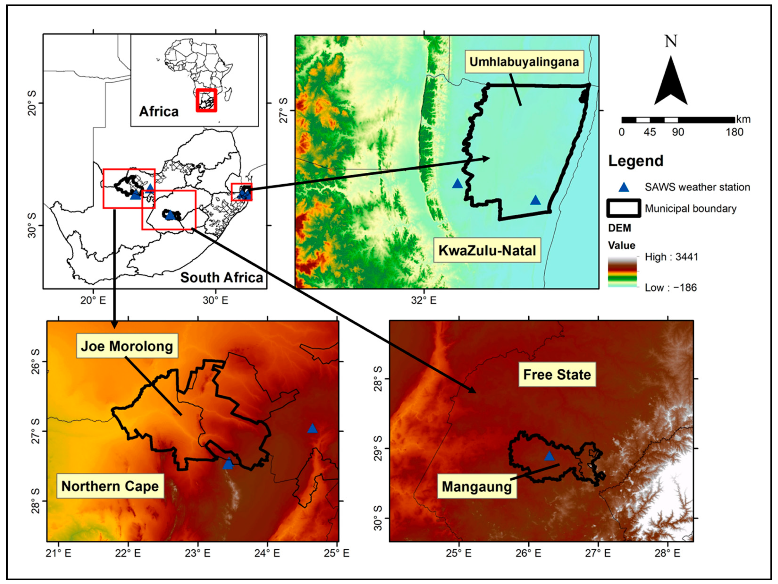
The study was conducted across three local municipalities (Umhlabuyalingana, Joe Morolong, and Mangaung) found in three provinces in South Africa (i.e., KwaZulu-Natal, Free State, and Northern Cape provinces) (Figure 1). The municipalities were selected based on two fundamental criteria: (i) the area is situated in a communal/former homeland area and (ii) there are small-scale subsistence farms/farmers, providing an opportunity to assess land use and land cover change in marginalized landscapes where small-scale and subsistence farming exist. Broadly, the case study areas were also chosen across rainfall, soil, vegetation, and agro-ecological potential gradients, allowing an opportunity to study the relationship between land cover change and biophysical factors. All case study areas consist of rain-fed and groundwater small-scale farming systems, and changes in rainfall amount have implications on the yield and growth of the crops planted. Furthermore, the study area is situated in areas with a varying topography and different vegetation types, dominated by Grassland, mixed Nama-Karoo, and pockets of Savanna [20]. The selected local municipalities consist of rural areas with residents from different cultural backgrounds and political histories. Moreover, a portion of each study area is within the boundaries of former apartheid homelands (i.e., KwaZulu and Bophuthatswana). The common farming activities in these areas include livestock farming of cattle, goats, and sheep and crop farming of maize, beans, and other vegetables.
Rural areas in South Africa occur in both former apartheid homelands and non-homeland areas. Former homelands comprise 13% of South Africa’s land area and have a high population density, with activities such as small-scale agricultural practices for subsistence purposes forming part of their livelihood strategies [21,22,23]. Former homelands (also known as Bantustans) were a result of the apartheid government’s 1951 Bantu Authorities Act, which saw South Africa being divided into ten ethnically defined homelands, namely Transkei, Bophuthatswana, Venda, Ciskei, Gazunkulu, Lebowa, QwaQwa, KaNgwana, KwaNdebele, and KwaZulu [23]. Although these designations were changed after the transition to democracy in 1994, the legacy is still seen in the landscapes today with poorly performing local municipalities, high-density living conditions, and high natural resource extraction for subsistence use [21,22,24]. Studies in rural areas found in former homelands in South Africa have indicated that smallholder farmers stop farming due to low production yields related to poor soil fertility and drought impacts [3], while other studies have recorded a shift away from land-based livelihood strategies as sources of income [25].
Our case study areas were selected because they provide an opportunity to assess small-scale crop farming over time in areas that were previously marginalized and relied on subsistence farming to sustain their livelihoods. Understanding the influence of climate variability on land use and land cover change is important for areas that are reliant on subsistence farming as the future climate is predicted to be harsh, and therefore, in order to have improved mitigation strategies for these communities, we need to understand the past and current influences. The farming practices in these landscapes are rain-fed, and extreme climatic events such as drought and flooding influence the patterns of farming practice. The Umhlabuyalingana landscape (KwaZulu) is predominantly located on nutrient-poor sandy soils, and thus, farming practices are concentrated in wetlands. Other land uses in the landscape include plantation forest activities, which are governed by the tribal authorities. The landscape in the Mangaung and Joe Morolong areas are found in the former Bophuthatswana. In Joe Morolong, the landscape is drier, and subsistence farming practices are concentrated in the eastern side of the landscape. In Mangaung, agriculture is widespread, with a high domination of large commercial farms.
2.2. Data Acquisition and Processing
2.2.1. Land Cover Data
Landsat data were used to derive land use and land cover (LULC) maps. Landsat imagery is widely and successfully used for many LULC change studies across the world. The moderate resolution (30 m) of the Landsat imagery necessitates the use of high-resolution imagery such as Google Earth and aerial photographs to generate training data for the classifier, as well as for validating the model. Using high-resolution imagery for training the classifier improves the performance of Landsat imagery in depicting various land cover types including small-scale croplands. The assessment of the LULC was conducted over the period between 1984 and 2022 to capture crop abandonment rather than field deactivation/activation, which is common in small-scale farming. The time frame selected was limited to the availability of Landsat imagery with fewer distortions such as line scans and high cloud cover. We were able to extract a 38-year period worth of data in which both pre- and post-apartheid era landscape patterns were captured by the imagery. The 38-year period was divided into five observational years (i.e., 1984, 1994, 2004, 2014, and 2022) with a ten-year gap between the analysis years, except for the recent observation period (i.e., between 2014 and 2022).
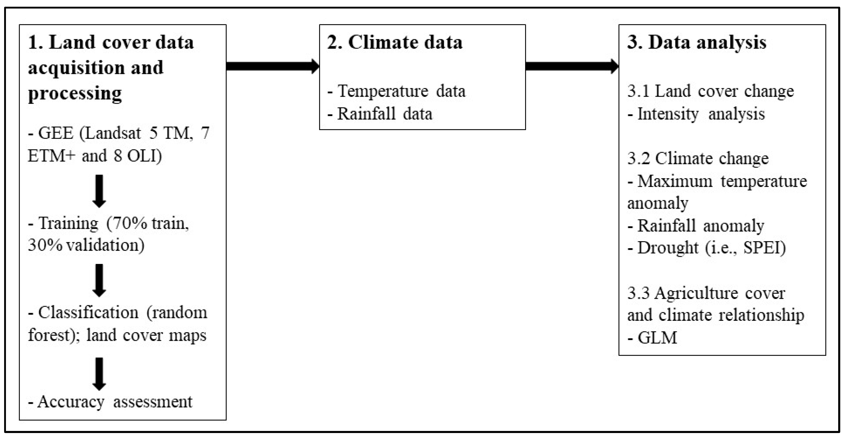
Processing of the remotely sensed data was performed in Google Earth Engine (GEE) following step 1 of the workflow in Figure 2. Google Earth Engine is a cloud-based platform that processes satellite imagery and other Earth observation and spatial data [26]. The GEE platform has a large number of datasets (including Landsat) readily available for use without having to download the images onto a hard drive, allowing users to conduct large-scale image processing, which normally requires higher computation power. The images are already rectified for radiometric and atmospheric distortions, and cloud-free images were used for classification; in a few special cases, cloud masking was applied to distorted pixels. A random forest (RF) classifier was used to classify LULC, and a total of 10 classes were categorized (Table 1). The random forest classifier performs better for image classification due to its robustness in discriminating pixel groupings, resulting in high classification accuracies [27]. Further image processing post-classification (such as fine-tuning) was performed in ArcMap 10.6. Image processing post-classification is important as it allows reclassification of the pixels that are incorrectly classified by applying expert knowledge of the landscape.
2.2.2. Climate Data
Climate data were obtained from the South African Weather Services (SAWS). The data contained daily rainfall (mm), as well as the minimum and maximum temperature (°C). The data were further converted into monthly and yearly rainfall and temperature to make the analysis easier. Data wrangling was performed to ensure that the data were consistent and accurate. The stations where the data were obtained are at the following locations: Maputaland (27.39°S, 32.18°E); Joe Morolong (27.47°S, 23.45°E; 27.43°S, 23.43°E); and Mangaung (29.1°S, 26.3°E).
2.3. Method
2.3.1. Land Cover Analysis
Land cover maps were produced using ArcMap 10.6 to demonstrate which land cover category was dominant in each landscape and time period, while showing how they changed through space and time. Trends of each land cover category were then analyzed by calculating the total area (km2) covered by each land cover category for each observation year. The total area of each land cover category was calculated by summing the area of individual patches belonging to a particular land cover category.
Land cover change was analyzed using the intensity analysis package in the R statistical software v 4.2.2. Intensity analysis is an open-source tool that is used for analyzing time series of land use and land cover change. The package can assess changes in land cover for data with both regular and irregular observation time intervals. Furthermore, the package computes a complete intensity analysis following the methods of Aldwaik and Pontius, [28]. The methods compute the rate of land cover change at three levels: (i) interval level: the overall size and annual rate of change in the landscape in each interval, classifying the rate as fast or slow against a uniform rate of change; (ii) categorical level: the overall size and intensity changes of gross gain and loss per land cover category, classifying the rate of gain or loss as active or dormant against a uniform rate of change; (iii) transitional level: the nature or pattern of size and intensity change per land cover category against the other land cover categories, classified as targeted or avoided compared to the uniform intensity if transitions were distributed uniformly [28].
2.3.2. Rainfall and Temperature
Rainfall and temperature data were analyzed in the R statistical software v 4.2.2, with mean temperature and total precipitation visualized graphically. Rainfall and temperature anomalies were used to indicate rainfall and temperature trends per annum compared to the overall mean of the study period. Anomalies were computed following Equations (1) and (2) for each year. A generalized linear model was used to perform trend analysis to determine the slope (change over time) and the significance of the trend.
where XR is the total annual rainfall and NR is the mean rainfall for the entire study period.
where Xtmax is the mean maximum temperature and Nt is the mean temperature for the entire study period.
Rainfall anomaly (mm) = XR − NR
Temperature anomaly (°C) = Xtmax − Nt
2.3.3. Drought
A drought proxy in the form of the Standardized Precipitation Evapotranspiration Index (SPEI) was used to quantify drought conditions and severity. The procedure to calculate the SPEI is similar to that of calculating the Standard Precipitation Index (SPI); however, the advantage of the SPEI is that it takes into account temperature variability [29]. The SPEI was developed through a combination of the Palmer Drought Severity Index (PDSI) and the multi-temporal ability of the SPI [30]. Standardized Precipitation Evapotranspiration Index calculations usually follow two methods, the Penman–Monteith [31] and the Thornthwaite [32]. For this study, the Thornthwaite equation was applied to compute the SPEI calculation because it is proven to show lower inter-annual variability compared to Penman’s method [33]. The SPEI was calculated at a time scale of 12, using a ‘rectangular’ kernel type, with 0 shift. The data were fit to a log-logistic distribution using the unbiased Probability-Weighted Moments (ub-pwm) parameter-fitting method. The SPEI has high fluctuations in short periods; however, these decrease as the time scale increases [8]. Because we were interested in annual changes over a 38-year period, an SPEI-12, which represents an annual drought analysis, was used. The SPEI was computed using climatic water balance, which is calculated by subtracting the potential evapotranspiration from the total rainfall. The SPEI values ranged between −2 and 2 with small values indicating the extent of dryness (droughts), while large values indicate the extent of wetness (Table 2). The SPEI was computed using the SPEI package (v1.8.0) [29] in R v 4.2.
2.3.4. Climate Variability Influence on Agricultural Land Cover
A generalized linear model (GLM) was used to unpack which of the climatic variables had a greater influence on the agricultural land cover patterns and the trend of change. Rainfall anomaly (mm), temperature anomaly (°C), and the SPEI were used as factors that could influence agricultural land change. The GLM model followed Equation (3), whereby agriculture land cover was the response variable to changes in climate factors. A Poisson regression family was used during the computation of the GLM because the nature of the agricultural land data is categorical (i.e., similar to counts). GLMs for each case study area were computed using the stats package in the R statistical software v 4.2.2.
whereby cropland area is the area covered by cropland in km2, RA is the rainfall anomaly, SPEI is the Standardized Precipitation Evapotranspiration Index, and MTA is the maximum temperature anomaly.
GLM = cropland area ~ RA + SPEI + MTA
3. Results
We assessed land use and land cover change over a period of 38 years in three local municipalities in South Africa. Our results demonstrated trends of declining grassland and agricultural land, while built up and woody vegetation have notably increased during the study period. The rate of intensity of change in the landscape varied across sites, with recent times being faster in Umhlabuyalingana and Joe Morolong areas. We further used agricultural land cover to demonstrate the influence of climate variability on land use change in rural landscapes, and the results indicated varying rainfall anomalies, characterized by below-normal rainfall and a reduced SPEI, indicating increased dryness. Furthermore, maximum temperatures were above normal at all three sites, particularly in the last two decades. The generalized linear models indicated that agricultural land change is significantly influenced by below-normal rainfall and increased dryness, while above-normal temperatures seemed to be more influential in the Joe Morolong landscape.
3.1. Land Cover Change Trends
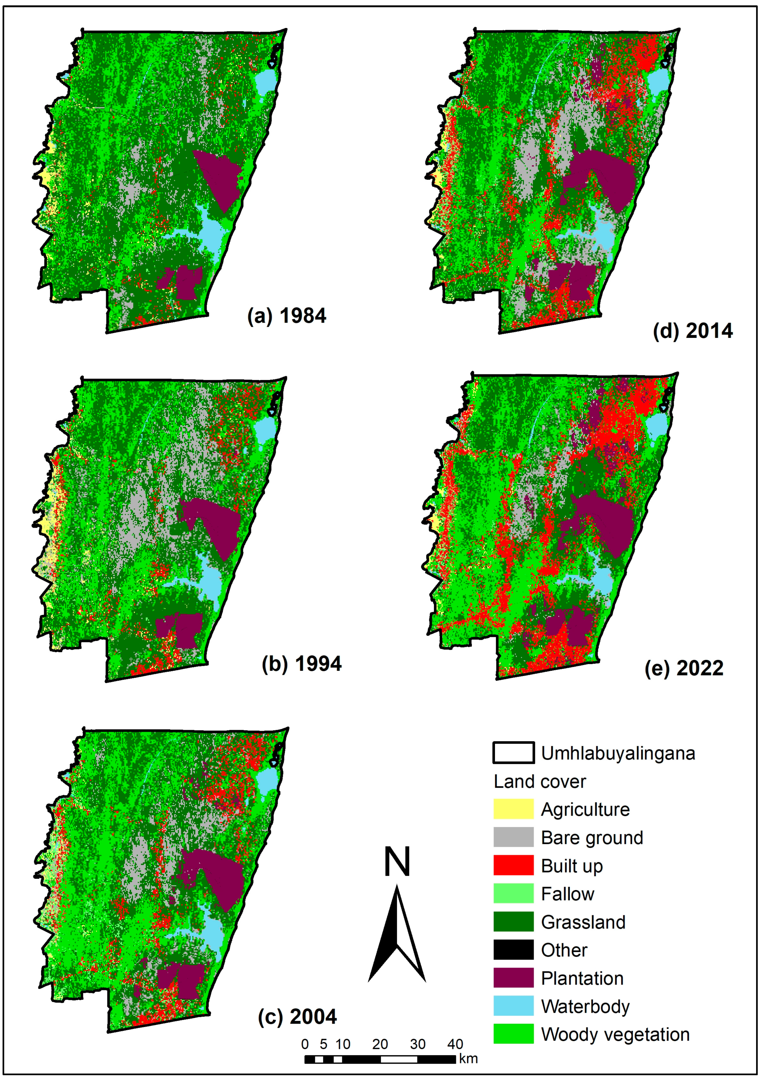
The patterns of land cover change were similar in all three case study areas, whereby all the landscapes were characterized by the dominance of natural vegetation (Figure 3, Figure 4 and Figure 5). Man-made land cover types such as built up and plantation were notably increasing in the Umhlabuyalingana landscape. In the Mangaung landscape, agricultural land was the notable change over time, with patches of this class changing to fallow.
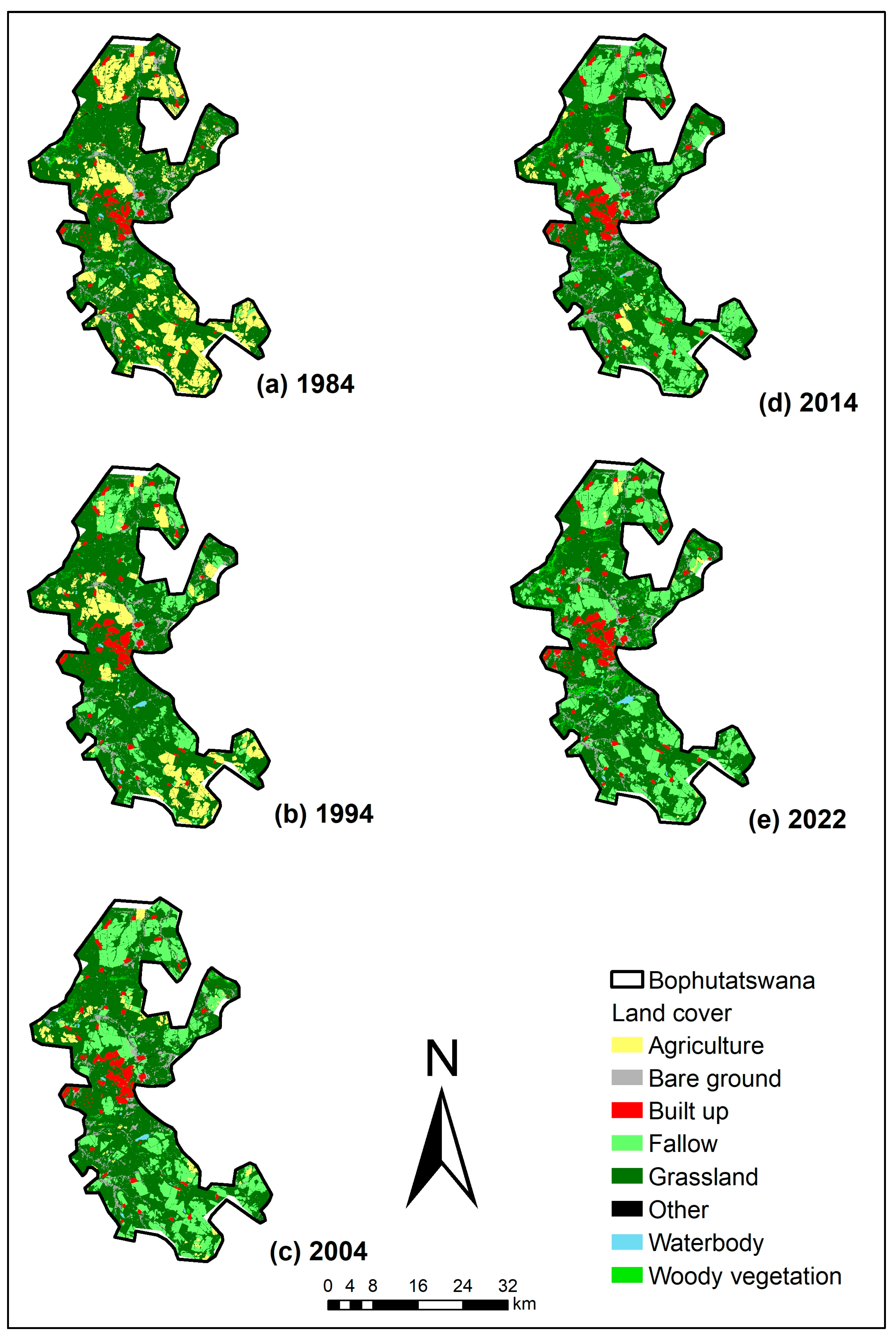
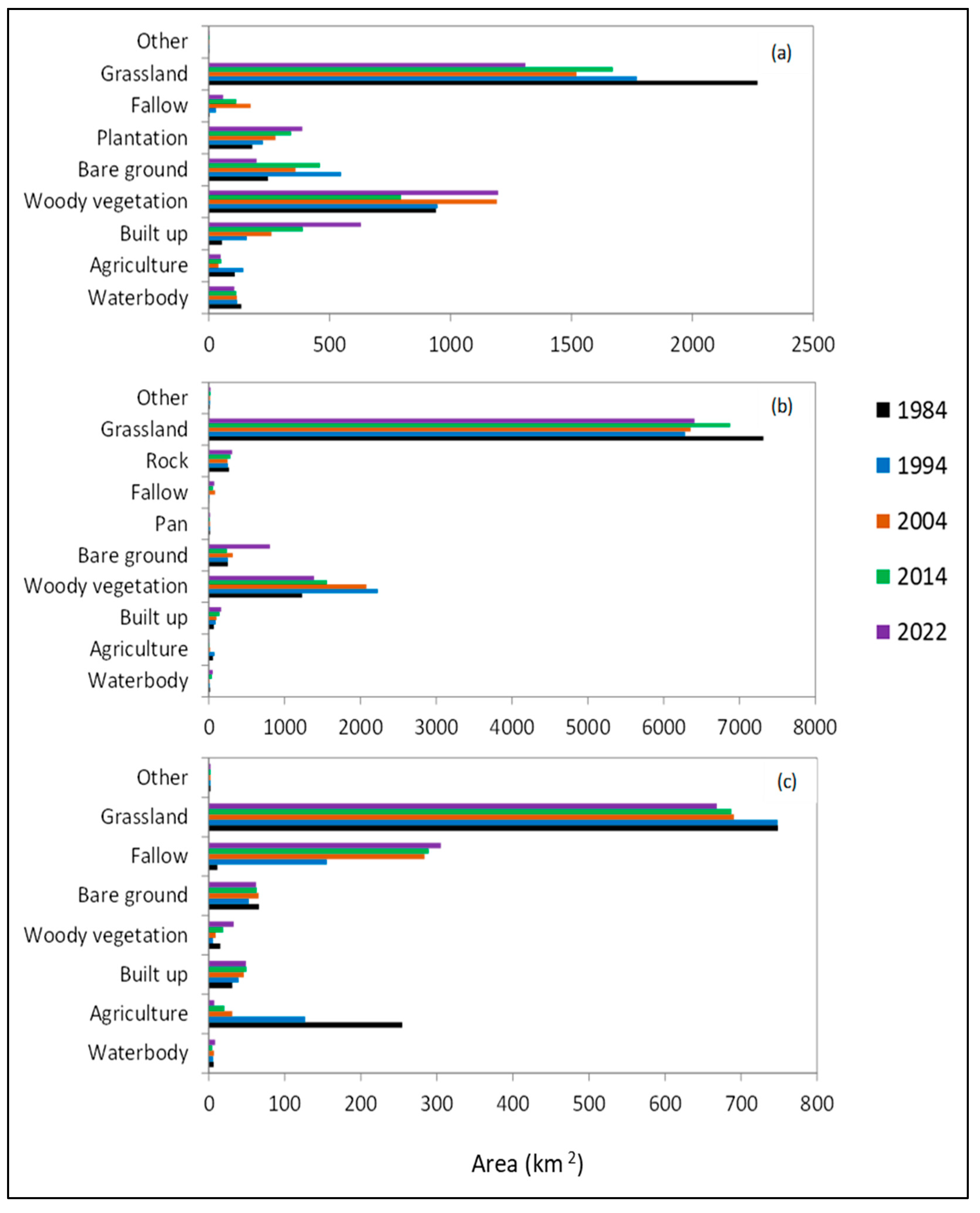
Grassland was the dominant cover at all three sites; however, it showed a declining trend over the study period (Figure 6a–c). Another common trend across the three sites was the substantial overall decline in the area covered by active agricultural land, while the area covered by fallow land increased. In Umhlabuyalingana, agricultural land area decreased from 107.5 km2 in 1984 to 49.5 km2 in 2022 (Figure 6a). In the Joe Morolong area, agricultural land area decreased from 54 km2 in 1984 to 1.6 km2 in 2022 (Figure 6b). In Mangaung, agricultural land area decreased from 254.6 km2 in 1984 to 7.1 km2 in 2022 (Figure 6c). Grassland remained the dominant land cover, although having declined, while there was a substantial increase in built up, woody vegetation, and plantation in Umhlabuyalingana over time (Figure 6a). The landscapes in Joe Morolong (Figure 6b) and Mangaung (Figure 6c) saw a gradual decline in grassland and a considerable decline in agricultural land (in Mangaung specifically).
3.2. Rate and Pattern of Land Cover Change
3.2.1. Interval Level
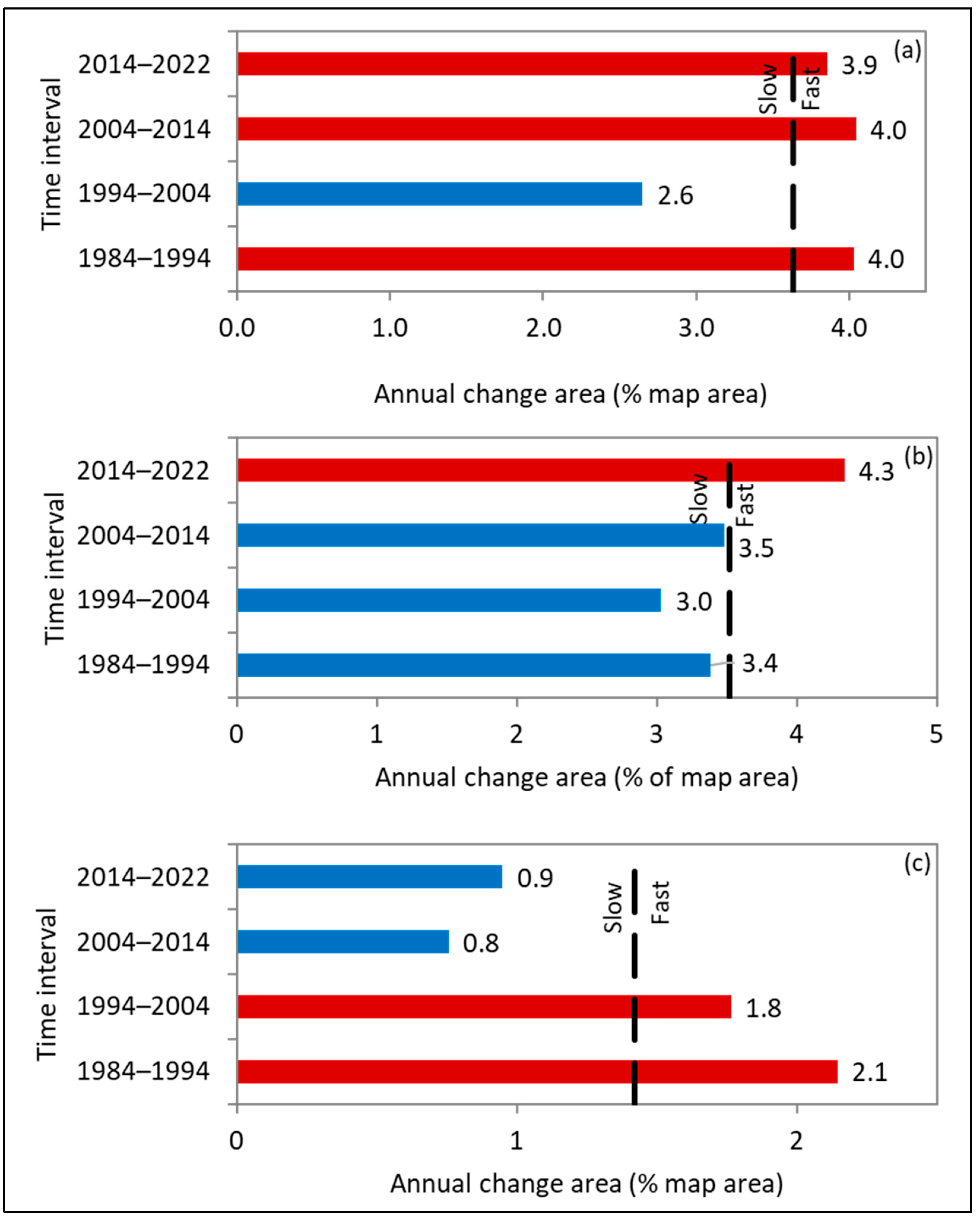
The rate of land cover change was variable at all three sites. In Umhlabuyalingana, the rate of change was fast (compared to the uniform rate of 3.6% per annum) in all the observation periods except for the period between 1994 and 2004 (Figure 7a). In Joe Morolong, the rate of change was slow (compared to the uniform rate of 3.5% per annum) in all the observation periods except for the period between 2014 and 2022 (Figure 7b). The landscape in the Mangaung area experienced a fast rate of change compared to the uniform rate of 1.4% per annum in the first two observation periods and a slow rate of change in the last two decades (Figure 7c).
3.2.2. Category Level
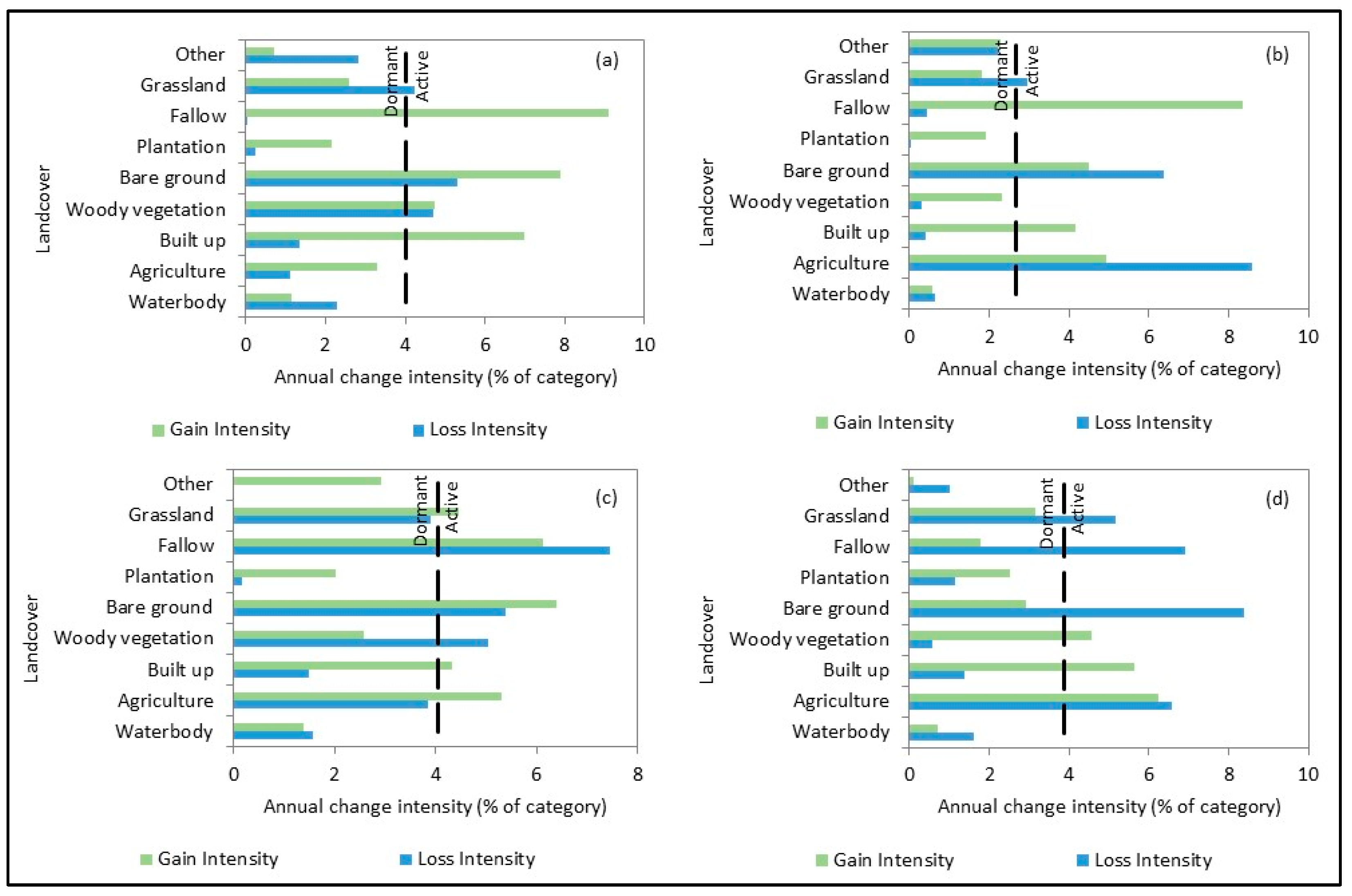
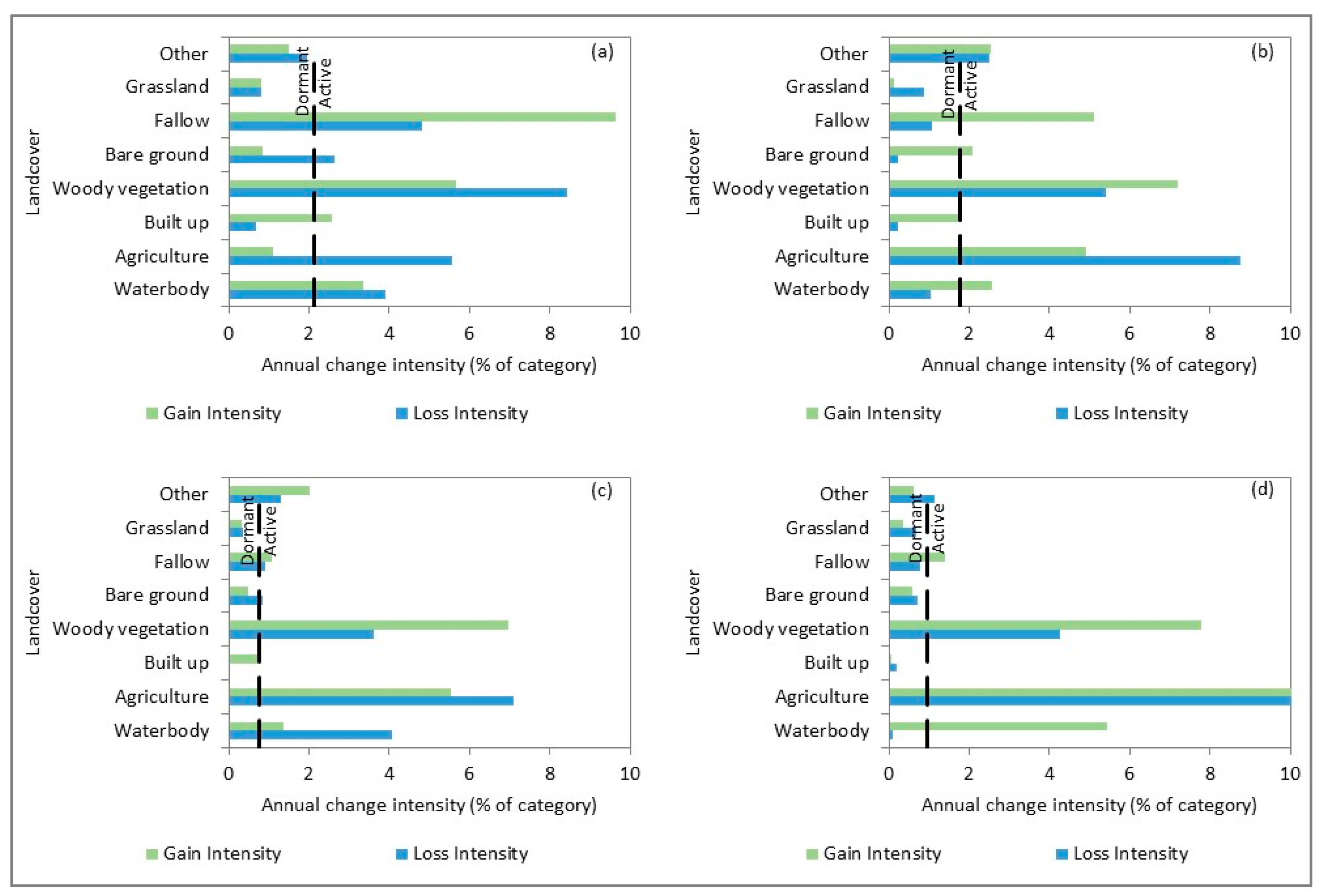
The nature of the change for each land cover category in the former homeland area in Umhlabuyalingana was characterized by active gains of fallow (in the first three time intervals), woody vegetation (two time periods), and built up areas (all time intervals). Grassland was characterized by active loss intensity during the analysis period, except for the 2004–2014 time interval, where it gained actively (Figure 8). Agriculture was dynamic, and this category showed active gain and loss; however, the loss intensity was greater than the gain, particularly between 1994–2004 and 2014–2022 (Figure 8b,d).
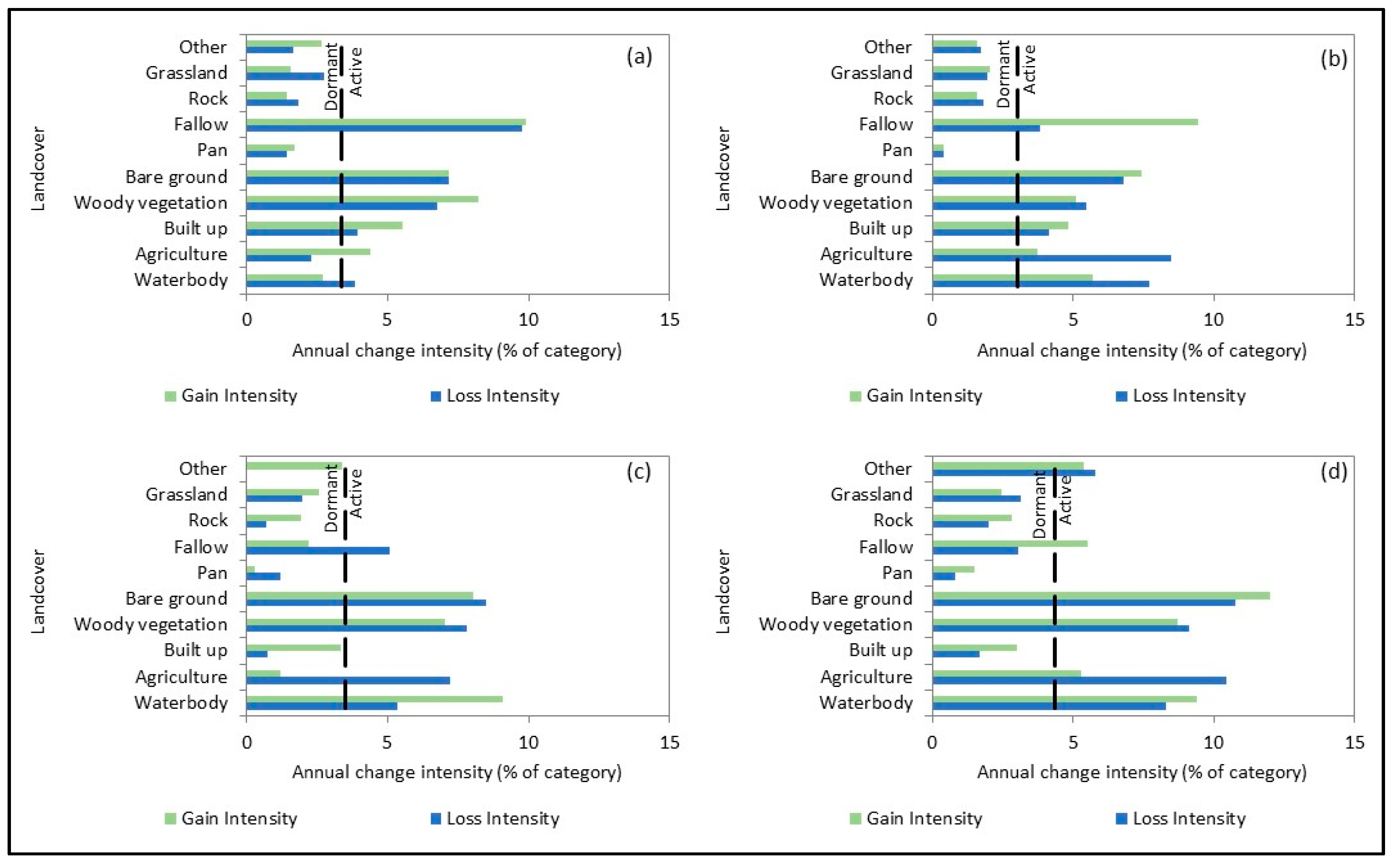
The former homeland area in the Joe Morolong area was characterized by dormant loss and gain of grassland, while exhibiting soil and water dynamics (i.e., existence of pans). Built up and woody vegetation gain intensities were active; however, woody vegetation also experienced active loss during the process (Figure 9). Agriculture was characterized by active loss intensity, which was greater than the gain, except for 1984 to 1994 (Figure 9a).
The former homeland area in Mangaung was characterized by dormant loss and gain intensity of grassland, while woody vegetation showed an active gain and loss for all the time intervals (Figure 10). Built up areas showed active gain for the first three time intervals, while from 2014–2022, the gain was not active (Figure 10d). Agriculture loss intensity was active and greater than the gain intensity (Figure 10).
3.2.3. Transitional Level
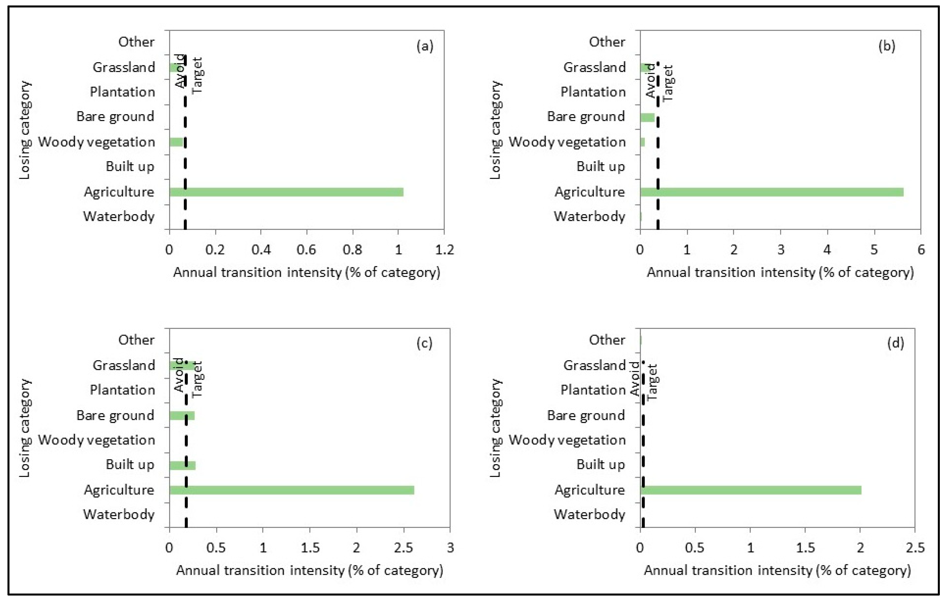
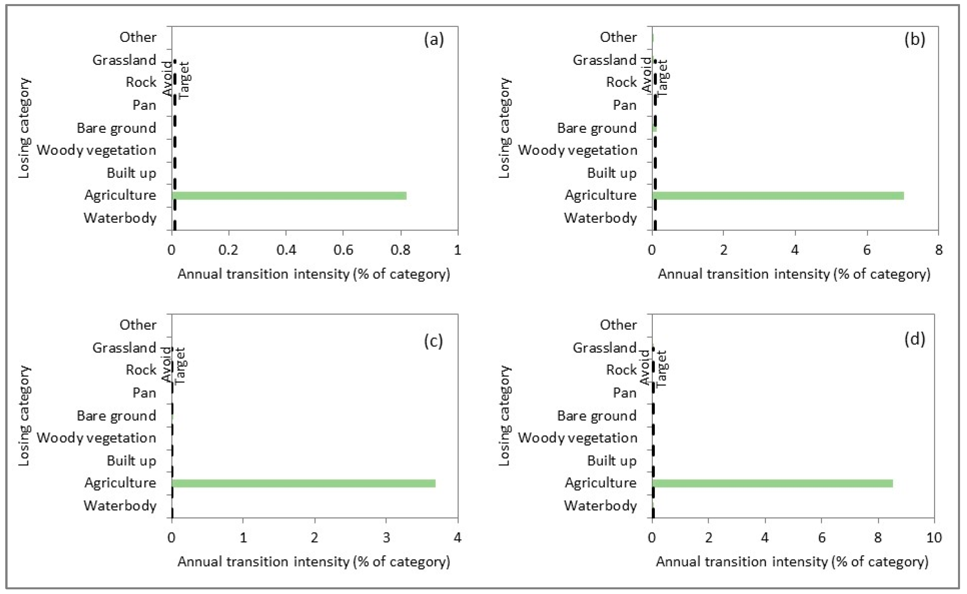
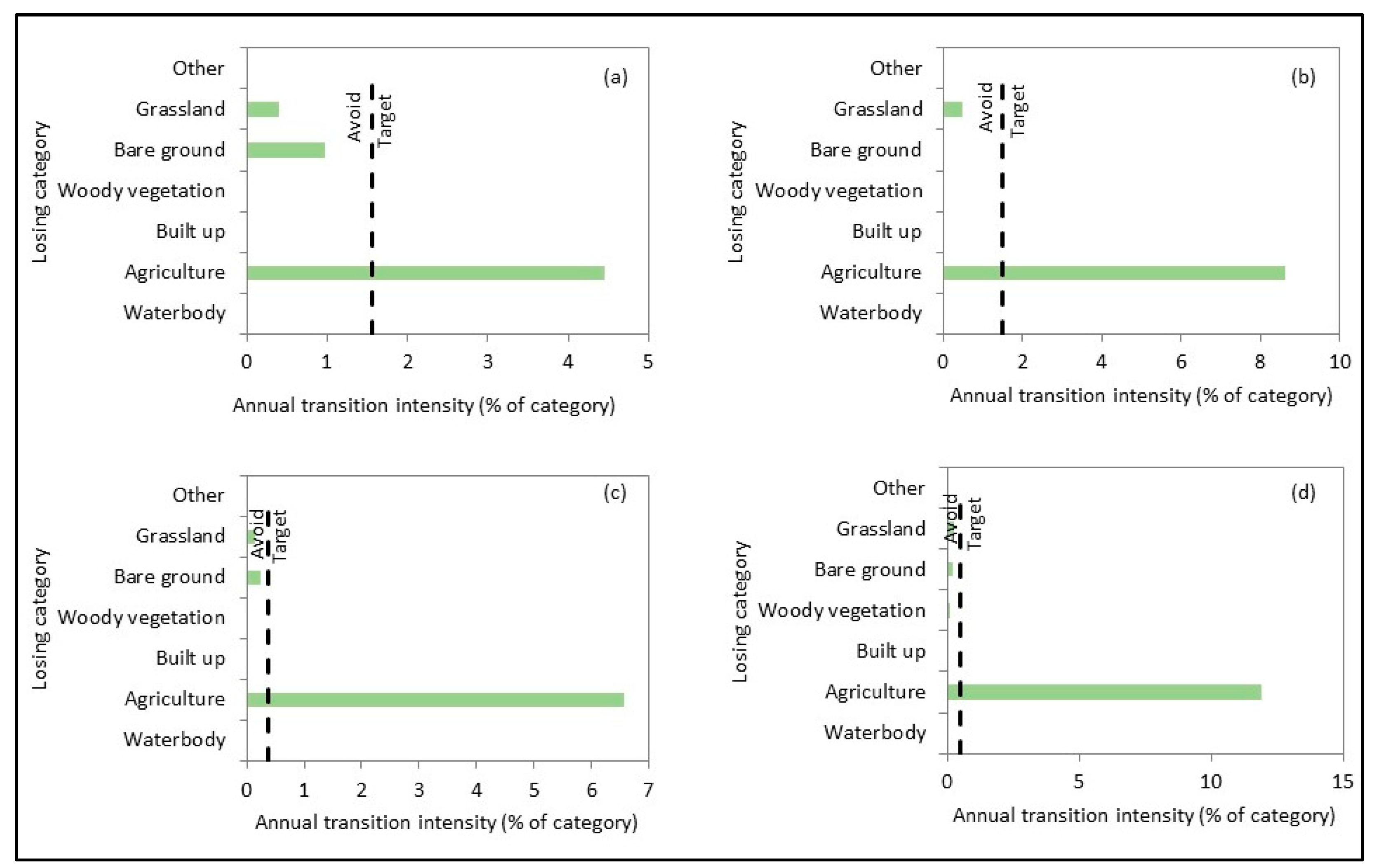
For the transition level, we interrogated the nature of agriculture change to assess which land cover category replaced agricultural land. The pattern of change was characterized by agricultural land transitioning to fallow lands at all three sites. The rate at which the transition from agricultural to fallow land was occurring was faster than the uniform rate in all three landscapes (Figure 11, Figure 12 and Figure 13).
3.3. Rainfall and Temperature Anomalies
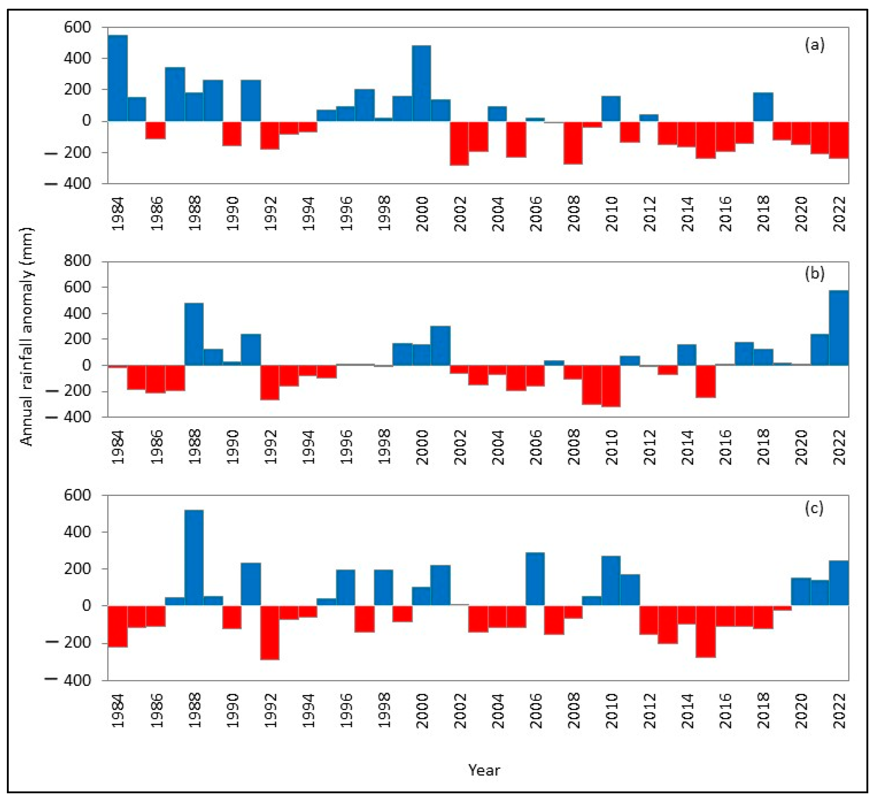
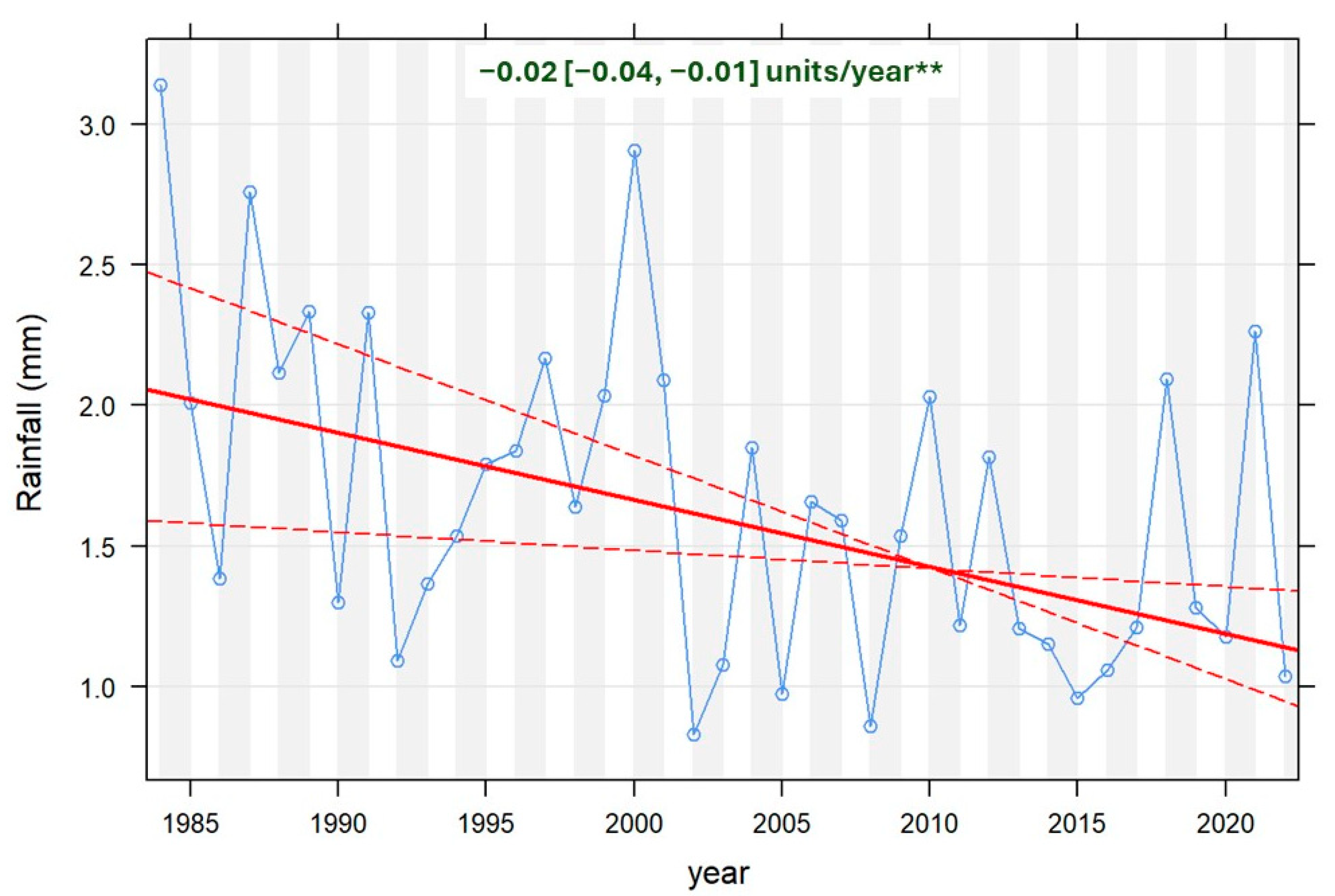
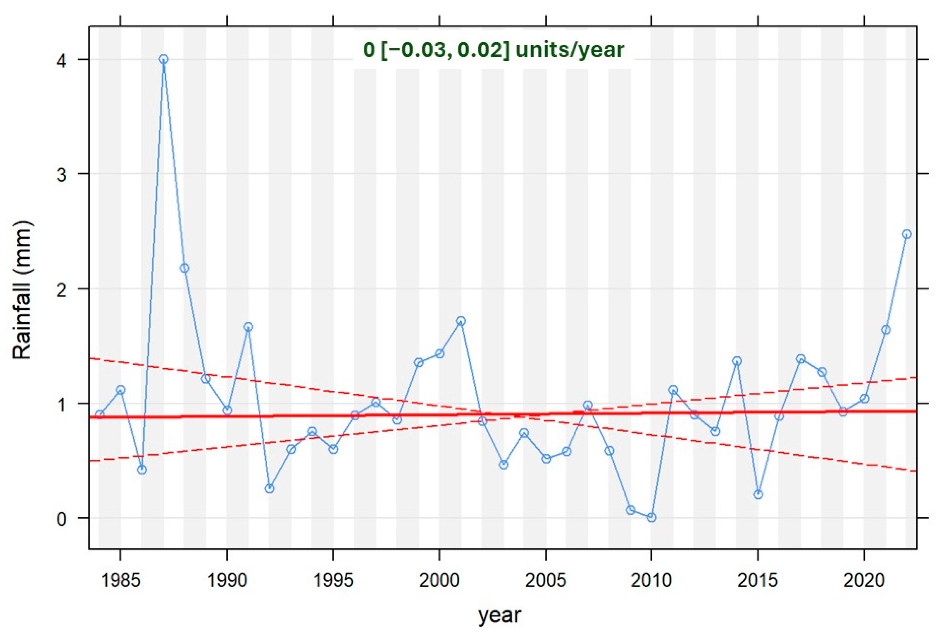
The annual rainfall anomaly was variable across the three sites. In the Umhlabuyalingana area, rainfall anomalies indicated that the last decade of the observation period received below-normal annual rainfall (Figure 14a), with a decrease of 0.02 mm/year (Appendix A: Figure A1). In the Joe Morolong area, rainfall was slightly above normal in the last decade of the observation period (Figure 14b); however, there was no significant change in the trend of the annual rainfall amount (Appendix A: Figure A2). In Mangaung, the last decade predominately received below-normal rainfall (Figure 14c), with no significant trend in rainfall change annually (Appendix A: Figure A3).
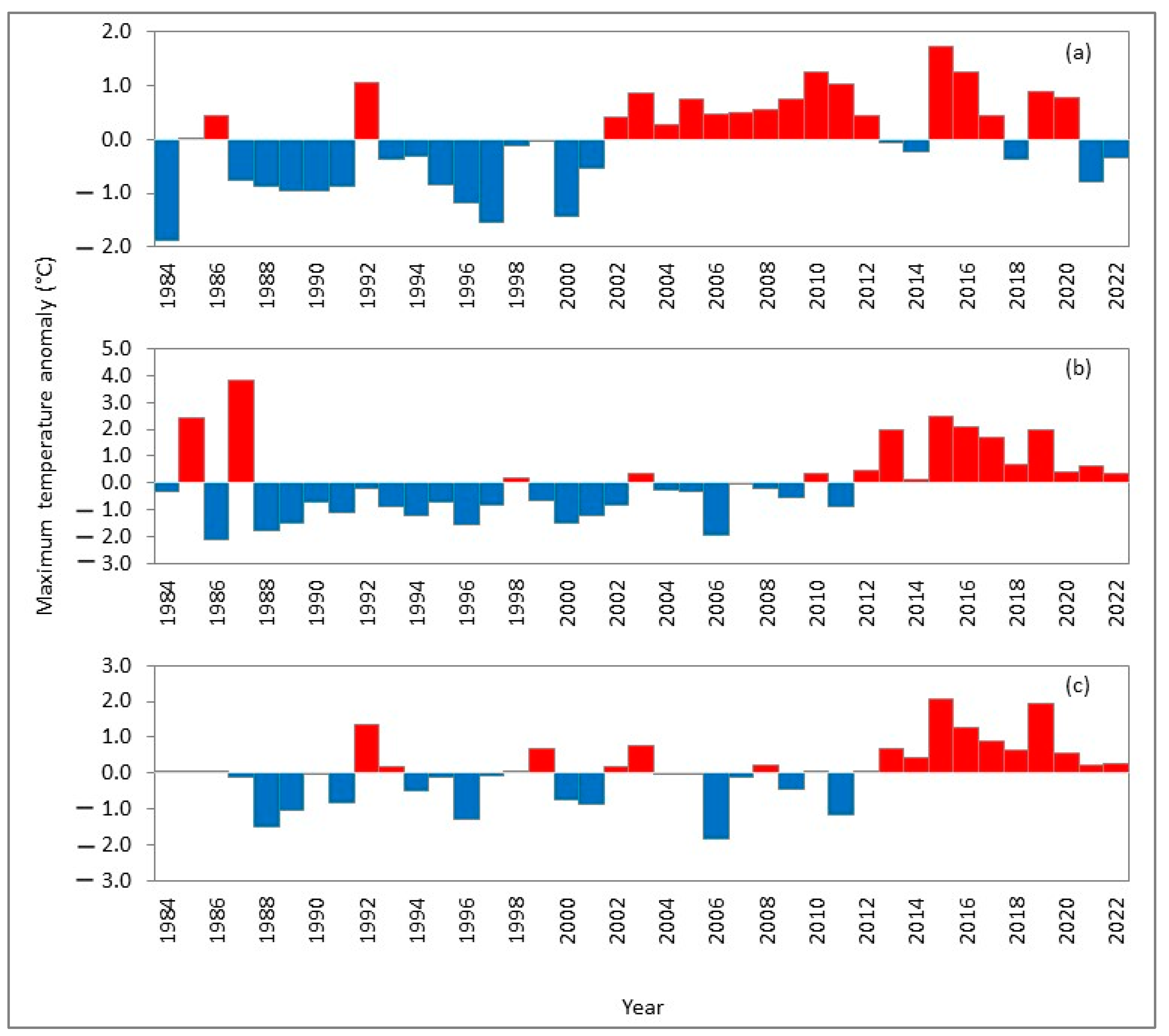
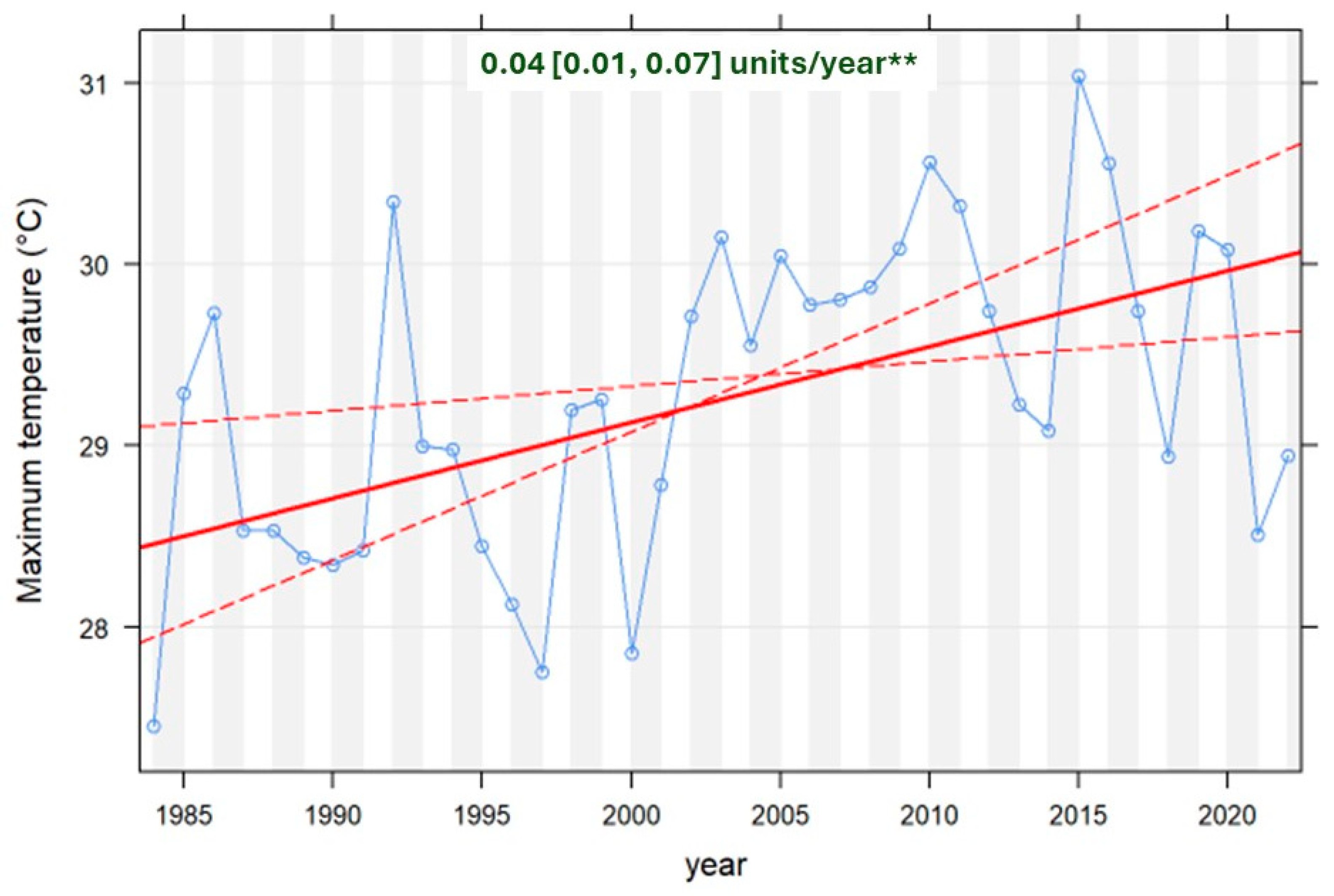
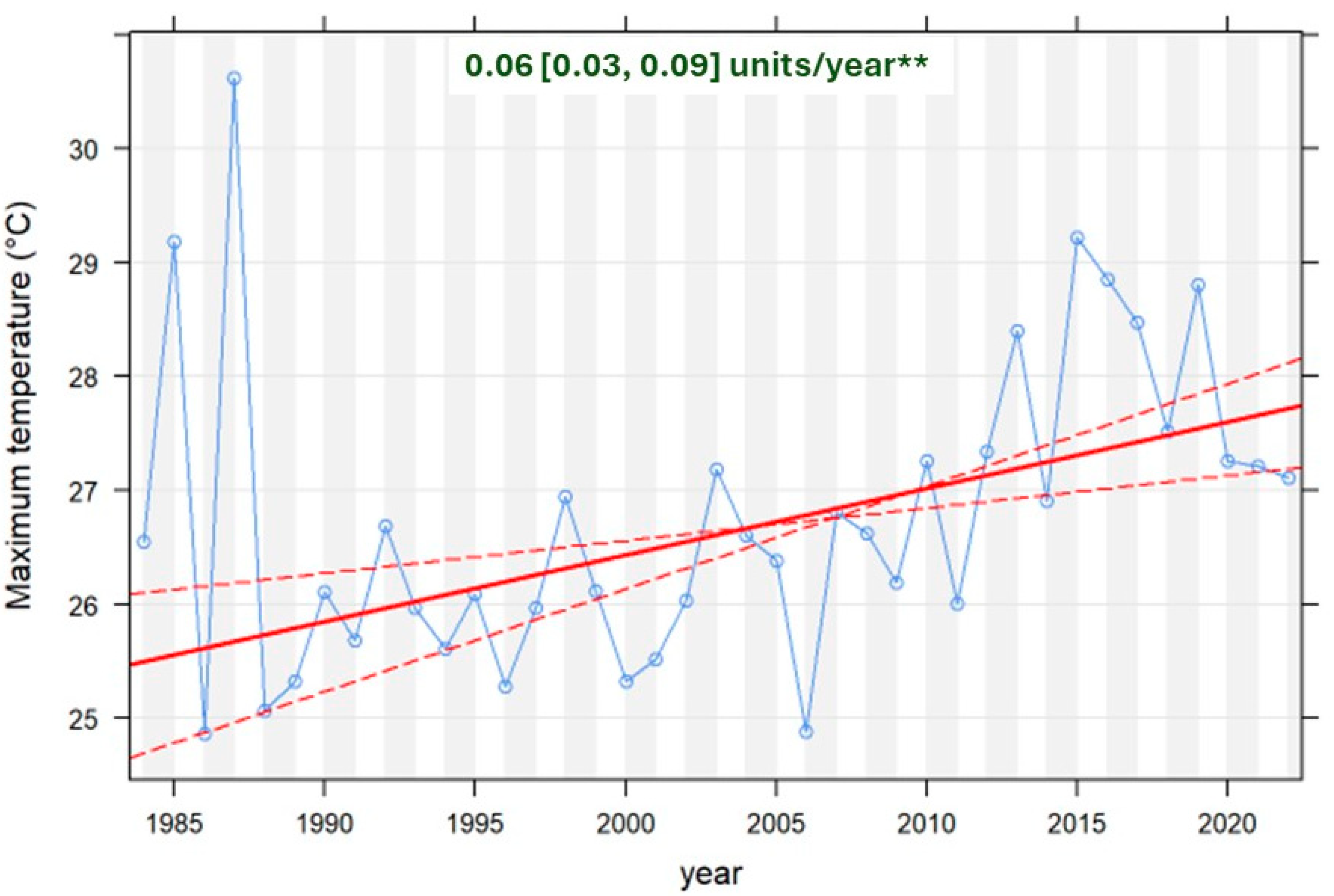
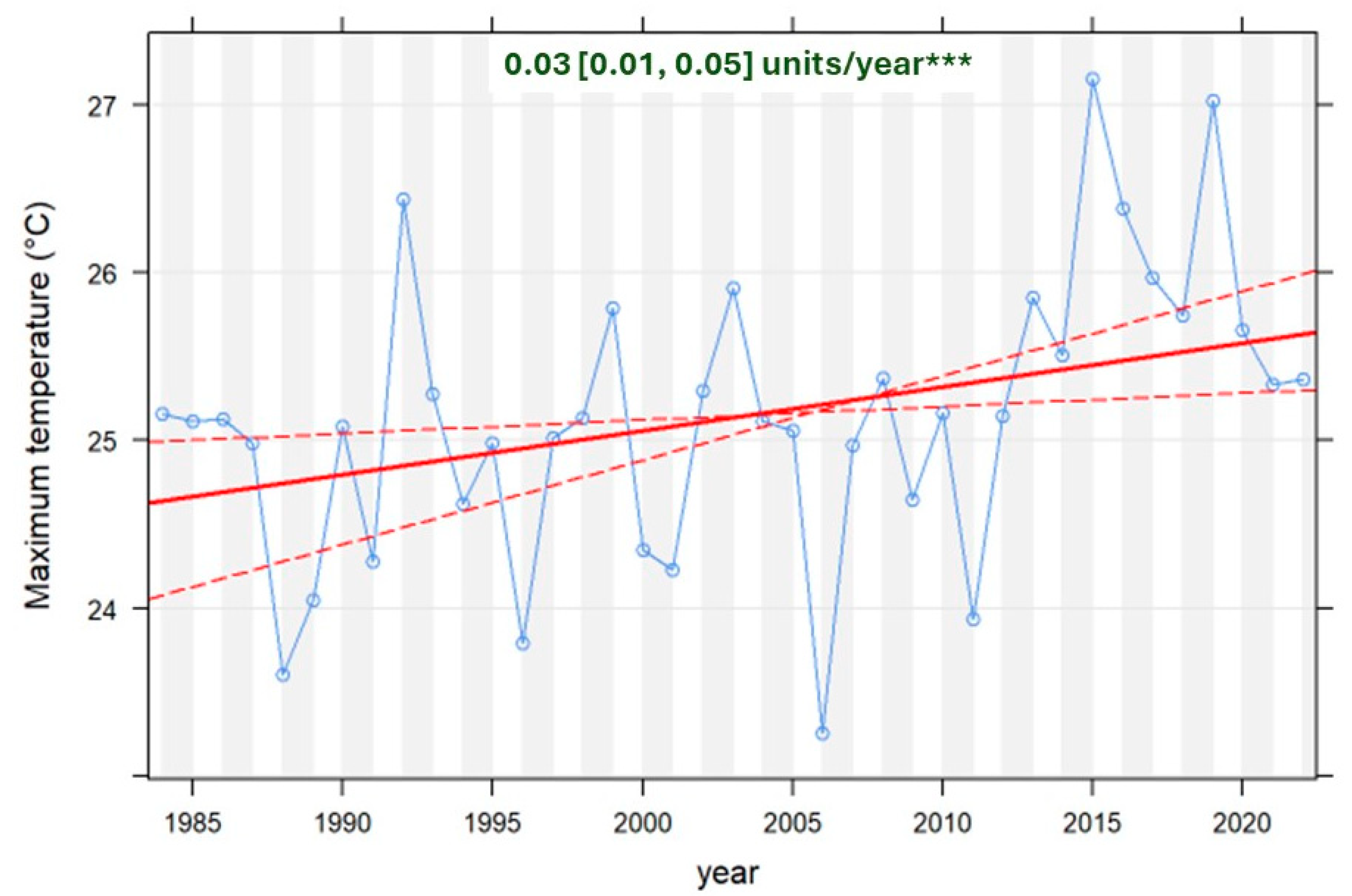
The maximum temperature indicated a similar pattern across the three sites, whereby the last decade of the observation period was warmer than average over the study period. The change in temperature has seen an increase of 0.04 °C per annum in Umhlabuyalingana (Figure 15a), 0.04 °C per annum in Joe Morolong (Figure 15b), and 0.03 °C per annum in Mangaung (Figure 15c). The trends were significantly increasing at all three sites, ranging between 0.3 °C and 0.6 °C per decade (Appendix A: Figure A4, Figure A5 and Figure A6).
3.4. Standardized Precipitation Evapotranspiration Index (SPEI)
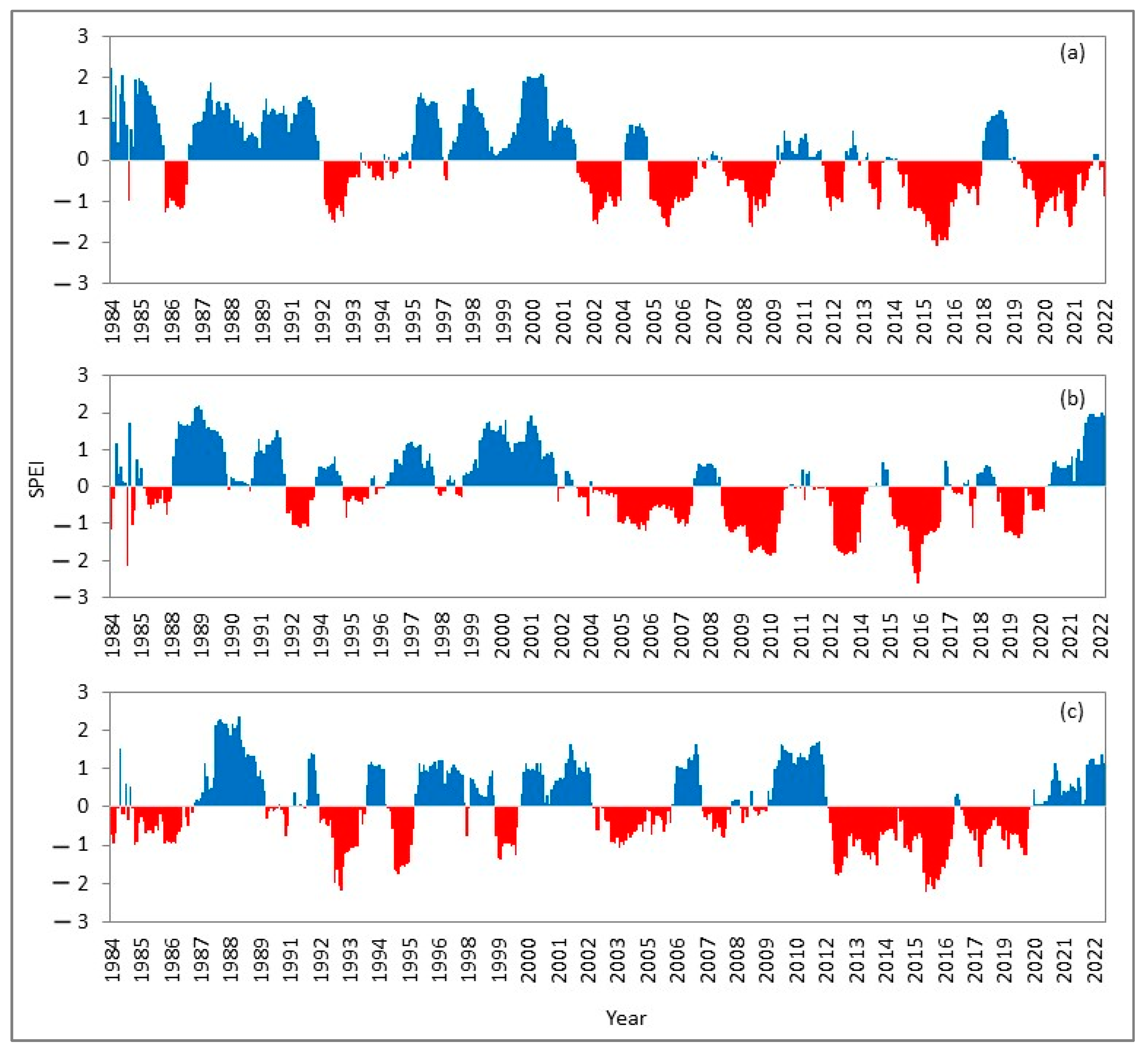
The Standardized Precipitation Evapotranspiration Index (SPEI) showed extended and frequent dry periods since 2002 in the Umhlabuyalingana area (Figure 16a). In the Joe Morolong area, dry periods were observed between 2002 and 2019, with improvements in wetness observed from 2020 to 2022 (Figure 16b). In the Mangaung area, wet and dry periods were irregular; however, a drought period was observed from 2012 until 2019 (Figure 16c).
3.5. Climate Variability Influence on Agricultural Land Change
The relationship between the change in agricultural land varied across sites; however, the SPEI was observed to be a significant variable influencing the reduction of the area utilized for agriculture (Table 3). In Umhlabuyalingana, all three climatic variables had a significant influence on agricultural land change (p < 0.05). In Joe Morolong, the rainfall anomaly did not have a strong influence on agricultural change (p > 0.05) and the maximum temperature anomaly, while the SPEI was shown to have a stronger significance (p < 0.05). In the Mangaung area, the rainfall anomaly and SPEI had an equally strong influence on agricultural land change over the study period (p < 0.05).
4. Discussion
4.1. Agricultural Land Change and Climate Variability
Areas utilized for agriculture declined over the study period in all the three case study areas (Umhlabuyalingana 58 km2, Joe Morolong 52.4 km2, and Mangaung 247.2 km2). The areas were replaced by fallow lands, indicating field deactivation. Agricultural land abandonment is a common practice in former homeland areas, and the literature has shown this trend in various parts of the country [3]. Shackleton et al. [34] showed that many households shifted to having gardens rather than owning large plots for crop farming, implying a change in farming strategy, which may help cope with extreme climate events such as drought. Ragie et al. [25] indicated that households in rural areas in Bushbuckridge, Mpumalanga province, South Africa, are shifting away from land-based livelihood strategies as a source of income, indicating that farming was becoming a less important livelihood strategy for rural households, resulting in the abandonment of croplands. Although our results showed a decline in large plots of agricultural land, we cannot know whether people are farming in small gardens or not as the resolution of the Landsat satellite imagery used is 30 m. The limitation of the medium resolution from Landsat propels future studies to use higher resolution imagery such as aerial photographs and Sentinel datasets to attempt small-scale crop mapping.
The rate of cropland loss was generally active for all three case study areas, indicating that the conversion rate is higher than the uniform rate of change. The results of the intensity analysis showed that agricultural land transitioned to fallow lands. Allowing a crop field to lie fallow is a common practice to allow the soil to recover nutrients; however, this change could also indicate land abandonment, where farmers are no longer using the field for crop farming purposes. In the case of land abandonment, natural vegetation tends to colonize these previously farmed areas.
The drivers of cropland abandonment are seemingly complex to quantify, mainly since the relationship between the patterns of cropland change and its drivers is non-linear; however, the decline in cropland in our study coincides with periods of extended and frequent dry conditions (i.e., decline in rainfall and increase in drought events). The generalized linear model indicated a strong correlation between cropland decline and the rainfall anomaly, maximum temperature anomaly, and SPEI in Umhlabuyalingana (p < 0.05), while in Joe Morolong, only the SPEI and maximum temperature anomaly were strong influencers of cropland change (p < 0.05). For the Mangaung area, the rainfall anomaly and SPEI had a significant influence on cropland change (p < 0.05). A study by Zaveri et al. [35] showed that cropland area increased during dry rainfall anomalies, accounting for approximately 9% of the global increase in cropland over the past two decades. These results are at a global scale, while our results are at a local scale, indicating that local and regional climate becomes important for understanding changes in land use and land cover, particularly agricultural changes. Our correlation results from the generalized linear models showed that the rainfall anomaly was significantly correlated with agricultural land change in high-rainfall areas (i.e., Umhlabuyalingana and Mangaung), with below-normal rainfall periods leading to reduced agricultural practices in recent times. In areas where rainfall is low (i.e., Joe Morolong), the maximum temperature also played a significant role in determining cropland farming change.
Although this study showed signs of the influence of climate variability on agricultural land change, we argue that the patterns and trends of agricultural change are potentially driven by a combination of multiple drivers including climate, socio-economic, and political factors. Since agricultural practices are directly linked to human activities, future studies need to consider understanding the relationship between agricultural change and socio-economic and political dynamics. The nature of the relationship is likely to be non-linear [36,37], and thus, more research is required to unpack the interactions of cultivation practices, climate variability, socio-economic, and political dynamics in order to create a resilient small-scale crop farming system in rural South Africa.
Moyo and Ravhuhali [38] showed that drought and rainfall variability are two of the many other factors that lead to the abandonment of agricultural land (cropland). Our results demonstrated that the nature of the interaction between climate variability and the change in agricultural land seems to behave differently in high- and low-rainfall areas. For areas that receive high rainfall, rainfall anomalies and drought events have a greater influence on agricultural land cover, whereas in areas that receive low rainfall, changes in maximum temperature (maximum temperature anomaly) and drought seem to have more influence on agricultural cropping. Although this may show the influence of climate variability on agricultural land change, we argue that the patterns and trends of agricultural land abandonment are potentially driven by a combination of drivers including socio-economic and political factors, whereby a change in rainfall influences decision making on whether to abandon land for agriculture or cultivate an extended area based on prevailing socio-economic conditions nested within the political climate [39]. The prevalence of dry spells can affect yield production by affecting the crop’s development stages, particularly for staple crops such as maize, beans, and potatoes [40]. Often, rural communities are vulnerable to extreme climatic events, as they do not have the necessary available resources (financial or social) to deal with climate variability. With the climate expected to become warmer in the future, small-scale crop farming faces a challenge that requires research attention in order to combat the possible negative effects on livelihoods in rural South Africa and other developing countries.
4.2. Overall Land Cover Change
Land cover change showed that the rural landscapes are dynamic, with a notable decrease in natural grassland and agricultural land, while the woody vegetation, built up, plantation, and fallow categories increased. These changes, particularly decreasing natural grassland, have implications for the biodiversity and ecosystem services, which are important for sustaining the livelihoods of the local people in rural areas [41,42,43]. A decline in agricultural land has far more direct impacts on livelihoods as products obtained from crop farming can be used for subsistence or to generate income [3]. The decline in this category followed frequent periods of dry conditions, where rainfall was below average and drought was prolonged, illustrating the influence that climate variability has on crop farming. Should the periods of prolonged dryness increase, small-scale farming practices will need to adapt to improve the resilience of crop farming in rural areas [41].
The land cover change results showed similar trends with a decline in natural grassland and agricultural land, with increased rates of change in certain time periods, which varied across the sites. At the category level, the loss of grassland was dormant in the Mangaung and Joe Morolong local municipalities, while it was active in Umhlabuyalingana. A dormant loss indicates that the conversion of grassland is lower than the uniform rate of change if the change was occurring randomly, while an active loss indicates the opposite. Moreover, the different rates of change in the landscape indicate the adaptability of rural dwellers to local conditions [37]. The observed decline in grassland is concerning as grasslands cannot be easily restored [44]. The results showed that grassland transitioned to woody vegetation and built up, indicating bush encroachment or thickening, as well as development taking place, which are signs of landscape degradation [45]. Various studies in rural South Africa have shown similar trends where natural grasslands declined over time while built up areas have increased [18,19]. Skowno et al. [46] have shown an increase in woodlands in various open landscapes in South Africa, with an annual increase of 0.22% between 1990 and 2013. The encroachment of woody plants in grasslands has implications for ecosystem functioning and ecosystem services, adding more pressure on grasslands [47]. With ever-increasing atmospheric carbon dioxide concentrations, woody plants are becoming favored over grass species [48], with low-income areas experiencing exacerbated land degradation from woody plants’ encroachment due to their reliance on natural resources [21,43,47,49].
Despite the encroachment of woody vegetation and development, other land cover categories such as plantation, in Umhlabuyalingana, have seen a remarkable increase over the 38-year period, driven by the economic value that comes from selling timber products. The market value of these products and the advantages they have for the local economy (and livelihood betterment) in this landscape need further investigation in order to inform management policies. Although there are financial benefits to the eucalyptus plantations in Umhlabuyalingana, the expansion of the plantations has negative impacts on the overall groundwater, given the landscape solely depends on rainfall and groundwater supply [16].
Our study assessed how climate variability influences changes in agricultural land change, paying special attention to changes in area covered by agricultural land and its relation to the rainfall anomaly, temperature anomaly, and Standardized Precipitation Evapotranspiration Index (SPEI). However, we understand that climate variability may also influence changes in other land cover types such as woody vegetation, grassland, and waterbodies. Therefore, future studies should pay attention to a suite of land cover categories to fully unpack the influence of climate variability on land cover change through space and time. We acknowledge the limitations of using one to two weather stations to represent a larger area; however, we aimed to use the only three in situ weather stations with a high accuracy of data. Therefore, future work should consider the use of modelled climate data for a wider spatial distribution, which could perhaps account for microclimatic variability.
5. Conclusions
We mapped and quantified changes in land use and land cover in marginalized landscapes over a period of 38 years. The rate of land cover change in the three rural South African landscapes was variable and site-specific, yet the patterns were similar with declines in grassland and agricultural land and the expansion of the woody vegetation, built up, plantation, and fallow categories. Loss of natural grassland indicates potential landscape degradation, where biodiversity and ecosystem services may be affected. Agricultural land change showed a significant decline over the study period, implying that the practice is becoming less important for rural communities in South Africa. The climate data showed varying trends in each case study area, with a general trend of declining annual rainfall and increased dryness, indicated by below-normal rainfall and a decreased SPEI in the last two decades. Maximum temperatures were above normal in all case study areas over the last two decades in Umhlabuyalingana and the last decade in both Joe Morolong and Mangaung areas. The decline in agricultural land area followed a period of below-normal rainfall, above-normal maximum temperature, and extended periods of dryness (i.e., drought). We argue that, although the change in agricultural land area followed the trends of climate variability, the different rates of change indicate complexity in this system with socio-economic and political dynamics influencing people’s adaptive abilities. Socio-ecological systems frameworks need to acknowledge and integrate the complexity of the various drivers of small-scale farming practices for more resilient and food-secure communities in rural areas.
Author Contributions
Conceptualization, B.P.M., W.T., G.T.F., H.V.d.M. and J.T.F.; methodology, B.P.M., W.T., G.T.F., H.V.d.M. and J.T.F.; software, B.P.M.; validation, B.P.M.; formal analysis, B.P.M.; Investigation, B.P.M.; resources, J.T.F.; data curation, B.P.M.; writing—original draft, B.P.M.; writing—review & editing, B.P.M., W.T., G.T.F., H.V.d.M. and J.T.F.; visualization, B.P.M.; supervision, B.P.M., W.T., G.T.F., H.V.d.M. and J.T.F.; project administration, B.P.M. and J.T.F.; funding acquisition, B.P.M. All authors have read and agreed to the published version of the manuscript.
Funding
The work was funded by the National Research Foundation (NRF) through the Scarce Skills Doctoral Scholarships, grant number 130043.
Data Availability Statement
All land cover data used for this research can be provided upon request to the authors. All climate data can be requested from the South African Weather Services. An example code script to perform the land cover classification used in this study can be found at https://code.earthengine.google.com/15cd09491b6d68d80650fb26c8c4257e (accessed on 12 March 2024), while all the analysis of the climate, intensity analysis, and agricultural relationships can be found on https://drive.google.com/drive/folders/103RF6Mvg3SZpg6P5uohZGScYbYSxljAC (accessed 12 March 2024).
Acknowledgments
We would also like to thank the South African Weather Services (SAWS) for providing us with the climate data. We would also like to thank the reviewers for their contributions to improving the manuscript.
Conflicts of Interest
The authors declare no conflicts of interest.
Appendix A
The Appendix contains figures showing the ThielSen trend analysis for the annual rainfall and maximum temperatures over the three case study areas.
Figure A1.
Annual rainfall trend for Umhlabuyalingana local municipality area, South Africa. The trend was produced using ThielSen trend analysis. The blue curve indicates the annual mean rainfall (mm). The solid red line shows the trend estimate and the dashed red lines show the 95% confidence intervals for the trend based on resampling methods. The ** in the figure indicates significance at the 0.01 confidence interval.

Figure A2.
Annual rainfall trend for Joe Morolong local municipality area, South Africa. The trend was produced using ThielSen trend analysis. The blue curve indicates the annual mean rainfall (mm). The solid red line shows the trend estimate and the dashed red lines show the 95% confidence intervals for the trend based on resampling methods.

Figure A3.
Annual rainfall trend for Mangaung local municipality area, South Africa. The trend was produced using ThielSen trend analysis. The blue curve indicates the annual mean rainfall (mm). The solid red line shows the trend estimate and the dashed red lines show the 95% confidence intervals for the trend based on resampling methods.

Figure A4.
Annual maximum temperature trend for Umhlabuyalingana local municipality area, South Africa. The trend was produced using ThielSen trend analysis. The blue curve indicates the annual maximum temperature (°C). The solid red line shows the trend estimate and the dashed red lines show the 95% confidence intervals for the trend based on resampling methods. The ** in the figure indicates significance at the 0.01 confidence level.

Figure A5.
Annual maximum temperature trend for Joe Morolong local municipality area, South Africa. The trend was produced using ThielSen trend analysis. The blue curve indicates the annual maximum temperature (°C). The solid red line shows the trend estimate and the dashed red lines show the 95% confidence intervals for the trend based on resampling methods. The ** in the figure indicates significance at the 0.01 confidence level.

Figure A6.
Annual maximum temperature trend for Mangaung local municipality area, South Africa. The trend was produced using ThielSen trend analysis. The blue curve indicates the annual maximum temperature (°C). The solid red line shows the trend estimate and the dashed red lines show the 95% confidence intervals for the trend based on resampling methods. The *** show that the trend is significant to the 0.001 confidence level.

References
- Morton, J.F. The impact of climate change on smallholder and subsistence agriculture. Proc. Natl. Acad. Sci. USA 2007, 104, 19680–19685. [Google Scholar] [CrossRef] [PubMed]
- Savo, V.; Lepofsky, D.; Benner, J.P.; Kohfeld, K.E.; Bailey, J.; Lertzman, K. Observations of climate change among subsistence-oriented communities around the world. Nat. Clim. Chang. 2016, 6, 462–473. [Google Scholar] [CrossRef]
- Blair, D.; Shackleton, C.M.; Mograbi, P.J. Cropland abandonment in South African smallholder communal lands: Land cover change (1950–2010) and farmer perceptions of contributing factors. Land 2018, 7, 121. [Google Scholar] [CrossRef]
- Hebinck, P.; Mtati, N.; Shackleton, C. More than just fields: Reframing deagrarianisation in landscapes and livelihoods. J. Rural Stud. 2018, 61, 323–334. [Google Scholar] [CrossRef]
- Pachauri, R.K.; Reisinger, A. IPCC Fourth Assessment Report; IPCC: Geneva, Switzerland, 2007; Volume 2007, p. 044023. [Google Scholar]
- Engelbrecht, F.; Adegoke, J.; Bopape, M.J.; Naidoo, M.; Garland, R.; Thatcher, M.; McGregor, J.; Katzfey, J.; Werner, M.; Ichoku, C.; et al. Projections of rapidly rising surface temperatures over Africa under low mitigation. Environ. Res. Lett. 2015, 10, 085004. [Google Scholar] [CrossRef]
- Blakeley, S.L.; Sweeney, S.; Husak, G.; Harrison, L.; Funk, C.; Peterson, P.; Osgood, D.E. Identifying precipitation and reference evapotranspiration trends in West Africa to support drought insurance. Remote Sens. 2020, 12, 2432. [Google Scholar] [CrossRef]
- Abu Arra, A.; Şişman, E. Characteristics of hydrological and meteorological drought based on intensity-duration-frequency (IDF) curves. Water 2023, 15, 3142. [Google Scholar] [CrossRef]
- Hayati, D.; Yazdanpanah, M.; Karbalaee, F. Coping with drought: The case of poor farmers of south Iran. Psychol. Dev. Soc. 2010, 22, 361–383. [Google Scholar] [CrossRef]
- van der Valk, M.; Keenan, P. Climate Change, Water Stress, Conflict and Migration; UNESCO: The Hague, The Netherlands, 2012. [Google Scholar]
- Eneyew, A.; Bekele, W. Determinants of livelihood strategies in Wolaita, southern Ethiopia. Agric. Res. Rev. 2012, 1, 153–161. [Google Scholar]
- Gebru, G.W.; Beyene, F. Rural household livelihood strategies in drought-prone areas: A case of Gulomekeda District, eastern zone of Tigray National Regional State, Ethiopia. J. Dev. Agric. Econ. 2012, 4, 158–168. [Google Scholar]
- Gonçalves, P.H.S.; da Cunha Melo, C.V.S.; de Assis Andrade, C.; de Oliveira, D.V.B.; de Moura Brito Junior, V.; Rito, K.F.; de Medeiros, P.M.; Albuquerque, U.P. Livelihood strategies and use of forest resources in a protected area in the Brazilian semiarid. Environ. Dev. Sustain. 2021, 24, 1–21. [Google Scholar] [CrossRef]
- Nkonki-Mandleni, B.; Ogunkoya, F.T.; Omotayo, A.O. Socioeconomic factors influencing livestock production among smallholder farmers in the free state province of south Africa. Int. J. Entrep. 2019, 23, 1–17. [Google Scholar]
- Kostov, P.; Lingard, J. Subsistence farming in transitional economies: Lessons from Bulgaria. J. Rural Stud. 2002, 18, 83–94. [Google Scholar] [CrossRef]
- Ramjeawon, M.; Demlie, M.; Toucher, M.L.; Janse van Rensburg, S. Analysis of three decades of land cover changes in the Maputaland Coastal Plain, South Africa. Koedoe Afr. Prot. Area Conserv. Sci. 2020, 62, a1642. [Google Scholar] [CrossRef]
- Rounsevell, M.D.A.; Ewert, F.; Reginster, I.; Leemans, R.; Carter, T.R. Future scenarios of European agricultural land use: II. Projecting changes in cropland and grassland. Agric. Ecosyst. Environ. 2005, 107, 117–135. [Google Scholar] [CrossRef]
- Jewitt, D.; Goodman, P.S.; Erasmus, B.F.; O’Connor, T.G.; Witkowski, E.T. Systematic land-cover change in KwaZulu-Natal, South Africa: Implications for biodiversity. S. Afr. J. Sci. 2015, 111, 1–9. [Google Scholar] [CrossRef] [PubMed]
- Mogonong, B.P.; Fisher, J.T.; Furniss, D.; Jewitt, D. Land cover change in marginalised landscapes of South Africa (1984–2014): Insights into the influence of socio-economic and political factors. S. Afr. J. Sci. 2023, 119, 1–10. [Google Scholar] [CrossRef] [PubMed]
- Mucina, L.; Rutherford, M. The Vegetation of South Africa, Lesotho and Swaziland; Strelitzia 19; Memoirs of the Botanical Survey of South Africa; South African National Biodiversity Institute: Pretoria, South Africa, 2006. [Google Scholar]
- Dovie, D.B.; Shackleton, C.M.; Witkowski, E. Valuation of communal area livestock benefits, rural livelihoods and related policy issues. Land Use Policy 2006, 23, 260–271. [Google Scholar] [CrossRef]
- Twine, W.; Saphugu, V.; Moshe, D. Harvesting of communal resources by ‘outsiders’ in rural South Africa: A case of xenophobia or a real threat to sustainability? Int. J. Sustain. Dev. World Ecol. 2003, 10, 263–274. [Google Scholar] [CrossRef]
- Ramutsindela, M. Resilient geographies: Land, boundaries and the consolidation of the former bantustans in post-1994 South Africa. Geogr. J. 2007, 173, 43–55. [Google Scholar] [CrossRef]
- Shackleton, C.; Shackleton, S. The importance of non-timber forest products in rural livelihood security and as safety nets: A review of evidence from South Africa. S. Afr. J. Sci. 2004, 100, 658–664. [Google Scholar]
- Ragie, F.H.; Olivier, D.W.; Hunter, L.M.; Erasmus, B.F.; Vogel, C.; Collinson, M.; Twine, W. A portfolio perspective of rural livelihoods in Bushbuckridge, South Africa. S. Afr. J. Sci. 2020, 116, 1–8. [Google Scholar] [CrossRef] [PubMed]
- Mutanga, O.; Kumar, L. Google earth engine applications. Remote Sens. 2019, 11, 591. [Google Scholar] [CrossRef]
- Belgiu, M.; Drăguţ, L. Random forest in remote sensing: A review of applications and future directions. ISPRS J. Photogramm. Remote Sens. 2016, 114, 24–31. [Google Scholar] [CrossRef]
- Aldwaik, S.Z.; Pontius, R.G., Jr. Intensity analysis to unify measurements of size and stationarity of land changes by interval, category, and transition. Landsc. Urban Plan. 2012, 106, 103–114. [Google Scholar] [CrossRef]
- Vicente-Serrano, S.M.; Beguería, S.; López-Moreno, J.I. A multiscalar drought index sensitive to global warming: The standardized precipitation evapotranspiration index. J. Clim. 2010, 23, 1696–1718. [Google Scholar] [CrossRef]
- Li, B.; Zhou, W.; Zhao, Y.; Ju, Q.; Yu, Z.; Liang, Z.; Acharya, K. Using the SPEI to assess recent climate change in the Yarlung Zangbo River Basin, South Tibet. Water 2015, 7, 5474–5486. [Google Scholar] [CrossRef]
- Penman, H.L. Natural evaporation from open water, bare soil and grass. Proc. R. Soc. Lond. Ser. A Math. Phys. Sci. 1948, 193, 120–145. [Google Scholar]
- Thornthwaite, C.W. An approach toward a rational classification of climate. Geogr. Rev. 1948, 38, 55–94. [Google Scholar] [CrossRef]
- Kumar, K.K.; Kumar, K.R.; Rakhecha, P. Comparison of Penman and Thornthwaite methods of estimating potential evapotranspiration for Indian conditions. Theor. Appl. Climatol. 1987, 38, 140–146. [Google Scholar] [CrossRef]
- Shackleton, C.; Mograbi, P.; Drimie, S.; Fay, D.; Hebinck, P.; Hoffman, M.; Maciejewski, K.; Twine, W. Deactivation of field cultivation in communal areas of South Africa: Patterns, drivers and socio-economic and ecological consequences. Land Use Policy 2019, 82, 686–699. [Google Scholar] [CrossRef]
- Zaveri, E.; Russ, J.; Damania, R. Rainfall anomalies are a significant driver of cropland expansion. Proc. Natl. Acad. Sci. USA 2020, 117, 10225–10233. [Google Scholar] [CrossRef] [PubMed]
- Giannecchini, M.; Twine, W.; Vogel, C. Land-cover change and human–environment interactions in a rural cultural landscape in South Africa. Geogr. J. 2007, 173, 26–42. [Google Scholar] [CrossRef]
- Ostrom, E. A general framework for analyzing sustainability of social-ecological systems. Science 2009, 325, 419–422. [Google Scholar] [CrossRef] [PubMed]
- Moyo, B.; Ravhuhali, K.E. Abandoned croplands: Drivers and secondary succession trajectories under livestock grazing in communal areas of South Africa. Sustainability 2022, 14, 6168. [Google Scholar] [CrossRef]
- Ebhuoma, E.E.; Donkor, F.K.; Ebhuoma, O.O.; Leonard, L.; Tantoh, H.B. Subsistence farmers’ differential vulnerability to drought in Mpumalanga province, South Africa: Under the political ecology spotlight. Cogent Soc. Sci. 2020, 6, 1792155. [Google Scholar] [CrossRef]
- Yengoh, G.T.; Armah, F.A.; Onumah, E.E.; Odoi, J.O. Trends in agriculturally-relevant rainfall characteristics for small-scale agriculture in Northern Ghana. J. Agric. Sci. 2010, 2, 3. [Google Scholar] [CrossRef]
- Lewis, D.; Bell, S.D.; Fay, J.; Bothi, K.L.; Gatere, L.; Kabila, M.; Mukamba, M.; Matokwani, E.; Mushimbalume, M.; Moraru, C.I.; et al. Community Markets for Conservation (COMACO) links biodiversity conservation with sustainable improvements in livelihoods and food production. Proc. Natl. Acad. Sci. USA 2011, 108, 13957–13962. [Google Scholar] [CrossRef]
- Nyaupane, G.P.; Poudel, S. Linkages among biodiversity, livelihood, and tourism. Ann. Tour. Res. 2011, 38, 1344–1366. [Google Scholar] [CrossRef]
- Cobbinah, P.B.; Black, R.; Thwaites, R. Biodiversity conservation and livelihoods in rural Ghana: Impacts and coping strategies. Environ. Dev. 2015, 15, 79–93. [Google Scholar] [CrossRef]
- Dudley, N.; Eufemia, L.; Fleckenstein, M.; Periago, M.E.; Petersen, I.; Timmers, J.F. Grasslands and savannahs in the UN Decade on Ecosystem Restoration. Restor. Ecol. 2020, 28, 1313–1317. [Google Scholar] [CrossRef]
- Venter, Z.S.; Scott, S.L.; Desmet, P.G.; Hoffman, M.T. Application of Landsat-derived vegetation trends over South Africa: Potential for monitoring land degradation and restoration. Ecol. Indic. 2020, 113, 106206. [Google Scholar] [CrossRef]
- Skowno, A.L.; Thompson, M.W.; Hiestermann, J.; Ripley, B.; West, A.G.; Bond, W.J. Woodland expansion in South African grassy biomes based on satellite observations (1990–2013): General patterns and potential drivers. Glob. Chang. Biol. 2017, 23, 2358–2369. [Google Scholar] [CrossRef] [PubMed]
- White, J.D.; Stevens, N.; Fisher, J.T.; Archibald, S.; Reynolds, C. Nature-reliant, low-income households face the highest rates of woody-plant encroachment in South Africa. People Nat. 2022, 4, 1020–1031. [Google Scholar] [CrossRef]
- Stevens, N.; Lehmann, C.E.R.; Murphy, B.P.; Durigan, G. Savanna woody encroachment is widespread across three continents. Glob. Chang. Biol. 2017, 23, 235–244. [Google Scholar] [CrossRef]
- Shackleton, C.M.; Shackleton, S.E. Household wealth status and natural resource use in the Kat River valley, South Africa. Ecol. Econ. 2006, 57, 306–317. [Google Scholar] [CrossRef]
Figure 1.
Locations of the selected local municipalities in KwaZulu-Natal, Free State, and Northern Cape provinces, South Africa.
Figure 1.
Locations of the selected local municipalities in KwaZulu-Natal, Free State, and Northern Cape provinces, South Africa.

Figure 2.
Graphical scheme summarizing the methodological approach and data used in the study.

Figure 3.
Land cover maps of Umhlabuyalingana former homeland area in KwaZulu-Natal province, South Africa.
Figure 3.
Land cover maps of Umhlabuyalingana former homeland area in KwaZulu-Natal province, South Africa.

Figure 4.
Land cover maps of Joe Morolong former homeland area in Northern Cape province, South Africa.
Figure 4.
Land cover maps of Joe Morolong former homeland area in Northern Cape province, South Africa.

Figure 5.
Land cover maps of Mangaung former homeland area in Free State province, South Africa.

Figure 6.
Area (km2) of each land cover category in the landscapes of the former homeland area found in (a) Umhlabuyalingana, (b) Joe Morolong and (c) Mangaung local municipalities, South Africa.
Figure 6.
Area (km2) of each land cover category in the landscapes of the former homeland area found in (a) Umhlabuyalingana, (b) Joe Morolong and (c) Mangaung local municipalities, South Africa.

Figure 7.
Annual change area for former homeland areas found in (a) Umhlabuyalingana, (b) Joe Morolong, and (c) Mangaung local municipalities, South Africa. The dashed line in the graphs shows the uniform rate of change, and if the bar falls left of the line, the change is slow, while if the bar is to the right of the line, the change is fast.

Figure 8.
Annual change intensity per category for (a) 1984–1994, (b) 1994–2004, (c) 2004–2014, and (d) 2014–2022 in the former homeland area found in Umhlabuyalingana local municipality, KwaZulu-Natal, South Africa. The dashed line in the graphs shows the uniform intensity, and if the bar falls left of the line, the intensity is dormant, while if the bar is to the right of the line, the intensity is active.

Figure 9.
Annual change intensity per category for (a) 1984–1994, (b) 1994–2004, (c) 2004–2014, and (d) 2014–2022 in the former homeland area found in Joe Morolong local municipality, Northern Cape, South Africa. The dashed line in the graphs shows the uniform intensity, and if the bar falls left of the line, the intensity is dormant, while if the bar is to the right of the line, the intensity is active.

Figure 10.
Annual change intensity per category for (a) 1984–1994, (b) 1994–2004, (c) 2004–2014, and (d) 2014–2022 in the former homeland area found in Mangaung local municipality, Free State, South Africa. The dashed line in the graphs shows the uniform intensity, and if the bar falls left of the line, the intensity is dormant, while if the bar is to the right of the line, the intensity is active.

Figure 11.
Annual change intensity of fallow gain against the other land cover categories in the landscape for (a) 1984–1994, (b) 1994–2004, (c) 2004–2014, and (d) 2014–2022 in the former homeland area found in Umhlabuyalingana local municipality, KwaZulu-Natal province, South Africa. The dashed line in the graphs shows the uniform intensity, and if the bar falls left of the line, the land cover is avoided, while if the bar is to the right of the line, the land cover is targeted.

Figure 12.
Annual change intensity of fallow gain against the other land cover categories in the landscape for (a) 1984–1994, (b) 1994–2004, (c) 2004–2014, and (d) 2014–2022 in the former homeland area found in Joe Morolong local municipality, Northern Cape province, South Africa. The dashed line in the graphs shows the uniform intensity, and if the bar falls left of the line, the land cover is avoided, while if the bar is to the right of the line, the land cover is targeted.

Figure 13.
Annual change intensity of fallow gain against the other land cover categories in the landscape for (a) 1984–1994, (b) 1994–2004, (c) 2004–2014, and (d) 2014–2022 in the former homeland area found in Mangaung local municipality, Free State province, South Africa. The dashed line in the graphs shows the uniform intensity, and if the bar falls left of the line, the land cover is avoided, while if the bar is to the right of the line, the land cover is targeted.

Figure 14.
Rainfall anomalies for the three South African Weather Service stations found at each case study site. (a) Umhlabuyalingana station, (b) Joe Morolong station, and (c) Mangaung station. Blue bars on the graph indicate above average rainfall, while red bars indicate below average rainfall against the mean rainfall for the entire study period.

Figure 15.
Maximum temperature anomalies for the three South African Weather Service stations found at each case study site. (a) Umhlabuyalingana station, (b) Joe Morolong station, and (c) Mangaung station. Blue bars on the graph indicate below average maximum temperature, while red bars indicate above average maximum temperature against the mean maximum temperature for the entire study period.

Figure 16.
The Standardized Precipitation Evapotranspiration Index (SPEI) of the (a) Umhlabuyalingana, (b) Joe Morolong, and (c) Mangaung areas between 1984 and 2022, South Africa. Negative values indicate a dry period (red bars), while positive values indicate a humid to wet period (blue bars).
Figure 16.
The Standardized Precipitation Evapotranspiration Index (SPEI) of the (a) Umhlabuyalingana, (b) Joe Morolong, and (c) Mangaung areas between 1984 and 2022, South Africa. Negative values indicate a dry period (red bars), while positive values indicate a humid to wet period (blue bars).


Table 1.
Land cover categories used for image classification in case study municipalities, South Africa.
Table 1.
Land cover categories used for image classification in case study municipalities, South Africa.
| Land Cover Category | Description |
|---|---|
| Waterbody | Surfaces covered by water such as rivers, lakes, and dams. |
| Agriculture | Areas that are actively cultivated, largely for subsistence purposes. |
| Built up | Urban and rural areas covered by man-made features such as buildings, representing human settlement. |
| Woody vegetation | Areas covered by natural or secondary woody vegetation such as woodlands and shrubland. |
| Grasslands | Areas that are covered by natural grasslands. |
| Bare ground | Areas of exposed soil, usually showing signs of erosion. |
| Pan | Dry flat areas covered by soil with a high salt concentration and temporarily inundated by water. |
| Plantation | Areas covered by planted trees, usually for commercial purposes. |
| Fallow | Areas that were previously farmed and are now covered by either secondary grasslands or woody vegetation. |
| Rock | Areas that are rocky and not covered by vegetation. |
| Other | Areas covered by other land cover classes such as roads and railways. |
Table 2.
Standardized Precipitation Evapotranspiration Index (SPEI) categories, adopted from Vicente-Serrano et al. [29].
Table 2.
Standardized Precipitation Evapotranspiration Index (SPEI) categories, adopted from Vicente-Serrano et al. [29].
| SPEI Values | Moisture Category |
|---|---|
| 2 and above | Extremely wet |
| 1.5 to 1.99 | Very wet |
| 1 to 1.49 | Moderately wet |
| −0.99 to 0.99 | Near normal |
| −1 to −1.49 | Moderately dry |
| −1.50 to −1.99 | Severely dry |
| −2 and less | Extremely dry |
Table 3.
Statistical outputs from the generalized linear models for the change in agricultural land in the three case study areas. SPEI = Standardized Precipitation Evapotranspiration Index.
Table 3.
Statistical outputs from the generalized linear models for the change in agricultural land in the three case study areas. SPEI = Standardized Precipitation Evapotranspiration Index.
| Case Study Area | Variable | Estimates | Std. Error | z-Value | p-Value |
|---|---|---|---|---|---|
| Umhlabuyalingana | Rainfall anomaly | 0.01 | 0.001 | 7.05 | <0.001 |
| SPEI | −3.08 | 0.39 | −7.84 | <0.001 | |
| Maximum temperature anomaly | 0.53 | 0.18 | 2.89 | 0.004 | |
| Joe Morolong | Rainfall anomaly | 0.01 | 0.004 | 1.59 | 0.11 |
| SPEI | −3.46 | 1.52 | −2.27 | 0.02 | |
| Maximum temperature anomaly | −3.74 | 1.22 | −3.07 | 0.002 | |
| Mangaung | Rainfall anomaly | −0.01 | 0.001 | −16.98 | <0.001 |
| SPEI | 1.56 | 0.22 | 7.10 | <0.001 | |
| Maximum temperature anomaly | 0.23 | 0.37 | 0.62 | 0.54 |
Disclaimer/Publisher’s Note: The statements, opinions and data contained in all publications are solely those of the individual author(s) and contributor(s) and not of MDPI and/or the editor(s). MDPI and/or the editor(s) disclaim responsibility for any injury to people or property resulting from any ideas, methods, instructions or products referred to in the content. |
© 2024 by the authors. Licensee MDPI, Basel, Switzerland. This article is an open access article distributed under the terms and conditions of the Creative Commons Attribution (CC BY) license (https://creativecommons.org/licenses/by/4.0/).
Share and Cite
MDPI and ACS Style
Mogonong, B.P.; Twine, W.; Feig, G.T.; Van der Merwe, H.; Fisher, J.T. Influences of Climate Variability on Land Use and Land Cover Change in Rural South Africa. Remote Sens. 2024, 16, 1200. https://doi.org/10.3390/rs16071200
AMA Style
Mogonong BP, Twine W, Feig GT, Van der Merwe H, Fisher JT. Influences of Climate Variability on Land Use and Land Cover Change in Rural South Africa. Remote Sensing. 2024; 16(7):1200. https://doi.org/10.3390/rs16071200
Chicago/Turabian StyleMogonong, Buster Percy, Wayne Twine, Gregor Timothy Feig, Helga Van der Merwe, and Jolene T. Fisher. 2024. "Influences of Climate Variability on Land Use and Land Cover Change in Rural South Africa" Remote Sensing 16, no. 7: 1200. https://doi.org/10.3390/rs16071200
Note that from the first issue of 2016, this journal uses article numbers instead of page numbers. See further details here.