Laser Backscattering Analytical Model of Doppler Power Spectra about Convex Quadric Bodies of Revolution during Precession

Abstract

In the realm of ballistic target analysis, micro-motion attributes, such as warhead precession, nutation, and decoy oscillations, play a pivotal role. This paper addresses these critical aspects by introducing an advanced analytical model for assessing the Doppler power spectra of convex quadric revolution bodies during precession. Our model is instrumental in calculating the Doppler shifts pertinent to both precession and swing cones. Additionally, it extends to delineate the Doppler power spectra for configurations involving cones and sphere–cone combinations. A key aspect of our study is the exploration of the effects exerted by geometric parameters and observation angles on the Doppler spectra, offering a comparative perspective of various micro-motion forms. The simulations distinctly demonstrate how different micro-motion patterns of a cone influence the Doppler power spectra and underscore the significance of geometric parameters and observational angles in shaping these spectra. This research not only contributes to enhancing LIDAR target identification methodologies but also lays a groundwork for future explorations into complex micro-motions like nutation.

1. Introduction

LIDAR technology plays an increasingly significant role in the field of environmental remote sensing. Its distinctive advantages, including a short wavelength, excellent beam collimation, and high brightness, have found extensive application in the military, aerospace, and remote sensing detection. LIDAR systems have the capability to perform target ranging and orientation based on laser scattering characteristics. Moreover, they can recognize target shape and posture by analyzing parameters such as position, radial velocity, micro-movement characteristics, and Doppler power spectra [1,2]. Simultaneously, radar technology’s Doppler techniques offer robust anti-interference capabilities in meteorological observations, significantly enhancing data collection accuracy, repeatability, and error reduction. Consequently, Doppler radar technology finds extensive application in meteorological observations and military domains. Doppler radar in meteorological observations typically employs fixed-frequency pulse waves for scanning. This allows for target detection even when the return frequency of the target differs from that of the transmitted wave. This technology is routinely employed for detecting atmospheric phenomena, enabling the monitoring of relative frequency changes in targets. It achieves this by tracking the time of pulse transmission and reception to continuously monitor target distance, thereby efficiently obtaining valuable data.

G. Pearson deployed a pulsed Doppler LIDAR in the tropical rain forest of Borneo to remotely monitor vertical and horizontal transport, aerosol distributions, and clouds in the lower levels of the atmosphere [3]. Pavlos Kollias utilized radar Doppler spectra observations to investigate liquid clouds that harbor drizzle droplets, typically occurring within specific atmospheric contexts characterized by elevated humidity levels, low cloud base temperatures, and enhanced vertical wind shear conditions [4].

Victor C. Chen used X-band radar to detect the triangle scatterers with vibration in 2000, and successfully obtained the micro-Doppler frequency shift in radar echoes through time–frequency transformation, then introduced the concept of the micro-Doppler effect into the microwave radar system for the first time. The research field of micro-Doppler feature extraction of a micro-moving target based on a microwave radar signal was developed. Later, Victor C. Chen used radar to detect pedestrians and conducted in-depth analysis and discussion on radar echo signals, which further demonstrated the huge application potential of the micro-Doppler effect in radar signal processing [5,6]. Yura and Bankman investigated the coherent and incoherent scattering of the target and conducted range Doppler imaging on the rotating cone to identify the micro-motion of the target [7]. Youmans estimated the Doppler centroid and Doppler width and proposed a preliminary model of a simple “reflective” cylinder [8]. Bankman [9] presented an analytical model of spectra in backscatter from the cone and cylinders rotating around their axes, which has the singular value problem. Gong YJ et al. proposed an analytical model of Doppler power spectra in backscatter from arbitrary rough convex quadric bodies of revolution (whose lateral surface is a quadric) rotating around axes [10]. In exploring the primary sources of turbulent mixing within the atmospheric boundary layer, Manninen et al. proposed a method using Doppler LIDAR data, which can detect the presence of turbulence [11]. This discovery provided an important perspective for understanding the dynamics of the atmospheric boundary layer. Similarly, Peng et al. introduced a Doppler LIDAR-based pedestrian detection and tracking scheme suitable for urban scenes. This scheme can simultaneously record the position and velocity of the target [12], which is of significant importance for traffic safety and surveillance in urban environments. Both studies showcase the potential applications of Doppler LIDAR technology in the fields of atmospheric science and urban safety, offering valuable technical references and prospects for this research.

The radar echoes of micro-motion targets reveal their intricate details, including structural, electromagnetic scattering, and motion characteristics. For this reason, the identification and detection of targets in space, air, ground, and sea, including ships, is of paramount importance [10,13,14,15]. In 2008, Victor C. Chen used the method of moments to simulate the precession echo data of the cone cylinder target, and analyzed the characteristics of micro-Doppler components corresponding to the spin and cone components as well as the micro-Doppler components corresponding to each scattering center of the cone [16]. Han Xun et al. proposed a method to distinguish spin, precession, and nutation forms by extracting features from the time–frequency distribution of the target echo [17]. Wang et al. [18] proposed a novel method for extracting precession parameters using coherent LIDAR based on a Doppler frequency profile (DFP) of dual-view observation, to the best of our knowledge. In 2018, Zhang Qun et al. [19] published a review of studies on the micro-Doppler effect, which summarized the micro-doppler model modeling, micro-Doppler feature extraction, micro-Doppler target imaging, and radar classification and recognition technology based on micro-Doppler features, and pointed out the future development direction of research on micro-Doppler feature extraction methods.

In the aforementioned study on micro-moving targets, Gong et al. [10] rigorously established the correlation between the Doppler shift of rotating targets and their coordinates within the laser band. The micro-motion is also an important form of motion of the target and has a nonnegligible influence on the Doppler power spectrum. By analyzing the Doppler power spectrum, it is also possible to determine the motion state of the object. Building upon their findings, this paper proposes research on micro-motions such as precession and swing, which have the potential to advance micro-motion detection, target recognition, and ground-based LIDAR detection.

2. Model of Space Precession Target

The target’s precession involves spinning around its axis of symmetry while also rotating around a specific axis in space. Translational flight is not taken into consideration in this particular model.

The convex quadric body of revolution, illuminated by one laser plane wave of wavelength $\lambda$ whose incidence direction is the z-direction, spins around its central axis $\stackrel{\rightharpoonup }{OT}$ with angular velocity $\omega$ while rotating around the precession axis $\stackrel{\rightharpoonup }{OP}$ with angular velocity ${\omega }_P$ (see Figure 1). The precession angle $\alpha$ represents the angle between $\stackrel{\rightharpoonup }{OT}$ and $\stackrel{\rightharpoonup }{OP}$. The angle between the line of sight (LOS) and $\stackrel{\rightharpoonup }{OP}$ is $\theta$. The observation angle $\gamma$ is the angle between the LOS and $\stackrel{\rightharpoonup }{OT}$. The axis $\stackrel{\rightharpoonup }{OT}$ and $\stackrel{\rightharpoonup }{OP}$ are both on the $yoz$ plane.

$$\begin{array}{l}\stackrel{\rightharpoonup }{OT}=(0,\sin \gamma ,\cos \gamma )\\ \stackrel{\rightharpoonup }{OP}=(0,\sin \theta ,\cos \theta )\end{array}$$

The Doppler shift of a precession cone is due to spin and rotation.

Rotating around $\stackrel{\rightharpoonup }{OP}$: For each point $r(x,y,z)$ on the lateral surface of the convex quadric body of revolution, the vector of angular velocity can be expressed as ${\stackrel{\rightharpoonup }{\Omega }}_p={\omega }_p\cdot \stackrel{\rightharpoonup }{OP}$, and its linear velocity ${\stackrel{\rightharpoonup }{v}}_P$ is given by:

$$\begin{array}{cc}{\stackrel{\rightharpoonup }{v}}_p& ={\stackrel{\rightharpoonup }{\Omega }}_p\times \stackrel{\rightharpoonup }{r}\\ & ={\omega }_p\cdot (0,\sin \theta ,\cos \theta )\times (x,y,z)\\ & ={\omega }_p\cdot (z\sin \theta -y\cos \theta ,x\cos \theta ,-x\sin \theta )\end{array}$$

(1)

Spinning around $\stackrel{\rightharpoonup }{OT}$: The coordinates of $\stackrel{\rightharpoonup }{OT}$ will change due to the spin, and the rotation matrix $M$ can be given by:

$$M=\left[\begin{array}{ccc}1& 0& 0\\ 0& \cos \theta & \sin \theta \\ 0& -\sin \theta & \cos \theta \end{array}\right]\left[\begin{array}{ccc}\cos ({\omega }_p\cdot t)& -\sin ({\omega }_p\cdot t)& 0\\ \sin ({\omega }_p\cdot t)& \cos ({\omega }_p\cdot t)& 0\\ 0& 0& 1\end{array}\right]\left[\begin{array}{ccc}1& 0& 0\\ 0& \cos \theta & -\sin \theta \\ 0& \sin \theta & \cos \theta \end{array}\right]$$

The coordinates of $\stackrel{\rightharpoonup }{OT}$ can be written as $\stackrel{\rightharpoonup }{O{T}^{\prime }}$, which is a function of time.

$$\begin{array}{ll}\stackrel{\rightharpoonup }{O{T}^{\prime }}& =M\cdot \stackrel{\rightharpoonup }{OT}\\ & =\left[\begin{array}{c}\sin ({\omega }_p\cdot t)\sin (\theta -\gamma )\\ \sin \gamma (\cos ({\omega }_p\cdot t){\cos }^2\theta +{\sin }^2\theta )+\cos \gamma \sin \theta \cos \theta (1-\cos ({\omega }_p\cdot t))\\ \cos \gamma \sin \theta \cos \theta (1-\cos ({\omega }_p\cdot t))+\cos \gamma (\cos ({\omega }_p\cdot t){\sin }^2\theta +{\cos }^2\theta )\end{array}\right]\end{array}$$

(2)

Let $\stackrel{\rightharpoonup }{O{T}^{\prime }}=(a,b,c)$, where:

$$\left[\begin{array}{c}a\\ b\\ c\end{array}\right]=\left[\begin{array}{c}\sin ({\omega }_p\cdot t)\sin (\theta -\gamma )\\ \sin \gamma (\cos ({\omega }_p\cdot t){\cos }^2\theta +{\sin }^2\theta )+\cos \gamma \sin \theta \cos \theta (1-\cos ({\omega }_p\cdot t))\\ \cos \gamma \sin \theta \cos \theta (1-\cos ({\omega }_p\cdot t))+\cos \gamma (\cos ({\omega }_p\cdot t){\sin }^2\theta +{\cos }^2\theta )\end{array}\right],$$

For each point $r(x,y,z)$ on the lateral surface of the convex quadric body of revolution, the vector of angular velocity can be expressed as ${\stackrel{\rightharpoonup }{\Omega }}_s=\omega \cdot \stackrel{\rightharpoonup }{O{T}^{\prime }}$, its linear velocity ${\stackrel{\rightharpoonup }{v}}_s$ is given by:

$$\begin{array}{ll}{\stackrel{\rightharpoonup }{v}}_s& ={\stackrel{\rightharpoonup }{\Omega }}_s\times \overrightarrow{r}\\ & =\omega \cdot (a,b,c)\times (x,y,z)\\ & =\omega \cdot (bz-cy,cx-az,ay-bx)\end{array}$$

(3)

So, the linear velocity of micro-motion of the cone can be measured by $\stackrel{\rightharpoonup }{v}$:

$$\stackrel{\rightharpoonup }{v}={\stackrel{\rightharpoonup }{v}}_p+{\stackrel{\rightharpoonup }{v}}_s$$

(4)

The direction of incidence of the laser can be expressed as $\stackrel{\rightharpoonup }{e}=(0,0,1)$ and the Doppler shift at each point on the surface of the cone in the backscattering direction is as follows:

$$\begin{array}{ll}\mathsf{\Delta }f& =-\frac{2(\stackrel{\rightharpoonup }{v}\cdot \stackrel{\rightharpoonup }{e})}{\lambda }\\ & =\frac{2{\omega }_{p}x\sin \theta }{\lambda }+\frac{2\omega (bx-ay)}{\lambda }\end{array}$$

(5)

If $\gamma =0°$, the equation of the lateral surface of the convex quadric body of revolution in the coordinate observation system is

$$x^2+y^2=A{z}^2+2Bz+C, z_0\le z\le z_0+h$$

(6)

where $h$ is the height of the convex quadrilateral of revolution. If $\gamma \ne 0°$, the observation angle $\gamma$ provides a clockwise rotation about the x-axis, and Equation (6) is transformed as follows:

$$x^2+{(y\cos \gamma -z\sin \gamma )}^2=A{(y\sin \gamma +z\cos \gamma )}^2+B(y\sin \gamma +z\cos \gamma )+C$$

(7)

According to the LIDAR equation

$$P=\frac{G_r{A}_r}{4\pi r_t^2{R}^2}{P}_t\frac{\sigma }{4\pi }$$

(8)

where $P$ is the received signal power, $P_t$ is the transmitter power, $\sigma$ is the effective target-scattering cross section, $A_r$ is the clear aperture of the detector, $G_r$ is the gain function, and $r_t,R$ are the distances from the target to the transmitter and receiver, respectively. The above situation applies when the laser beam is larger than the effective receiving area of the target object.

Let the surface element be $dA$, with zenith and azimuth angles of ${\theta }_i$ and ${\phi }_i$ in the incident direction, and zenith and azimuth angles of ${\theta }_s$ and ${\phi }_s$ in the scattering direction.

The backscattering power at each small section on the surface of the target can be written as

$$dP=K{f}_r(\beta ){\cos }^2\beta \frac{dxdy}{\left|\cos \beta \right|}$$

(9)

where $K=\frac{P_t{G}_r{A}_r}{4\pi r_t^2{R}^2}$, $dxdy$ is the area of each small section on the surface of the target.$f_r(\beta )$ is the bidirectional reflectance distribution function (BRDF), which depends on the material properties of the rough convex quadric body of revolution, and $\beta$ is the angle between the surface normal at that point and the opposite direction of the incidence direction of the laser. From Equation (7), the normal unit vector $\stackrel{\rightharpoonup }{n}$ at any point of the lateral surface can be obtained. The cosine of the angle between $\stackrel{\rightharpoonup }{n}$ and $-z$ is $\cos \beta$, which is expressed as:

$$\cos \beta =\frac{\sin \gamma (y\cos \gamma -z\sin \gamma )+\cos \gamma (Ay\sin \gamma +Az\cos \gamma +B)}{\sqrt{x^2+{(y\cos \gamma -z\sin \gamma )}^2+{(Ay\sin \gamma +Az\cos \gamma +B)}^2}}$$

(10)

The variable $z$ in Equation (10) can be expressed as a function of $x$ and $y$ from Equation (7). When the surface material is diffusely reflecting (Lambertian), the surface reflectance can be described by $f_r(\beta )=\rho /\pi$, where $\rho$ is the hemispherical reflectance, the value $K_L{=Kf}_r(\beta )$ is normalized to unity. Equation (9) is transformed as follows:

$$P(x,y)=K_L{\displaystyle \underset{z\in C}{\int }\cos \beta dxdy}$$

(11)

where the integral domain $C$ for a convex quadric body of revolution can be summarized as:

$$C:\begin{array}{c}\cos \beta >0\\ z_0\le y\sin \gamma +z\cos \gamma \le z_0+h\end{array}\begin{array}{c}\\ \end{array}\}$$

(12)

From Equations (5) and (11), both $P(x,y)$ and $\mathsf{\Delta }f$ are expressed as a function of $x$ and $y$, and each small section $(x,y)$ on the surface of the target can calculate received signal power $P(x,y)$ and Doppler shift $\mathsf{\Delta }f$. Thus, a plot can be drawn with $\mathsf{\Delta }f$ as the horizontal coordinate and $P(x,y)$ as the vertical coordinate; the resulting image is the laser backscattering Doppler spectrum subsequent modeling, and simulation calculations are also implemented based on this.

3. Simulations and Discussion

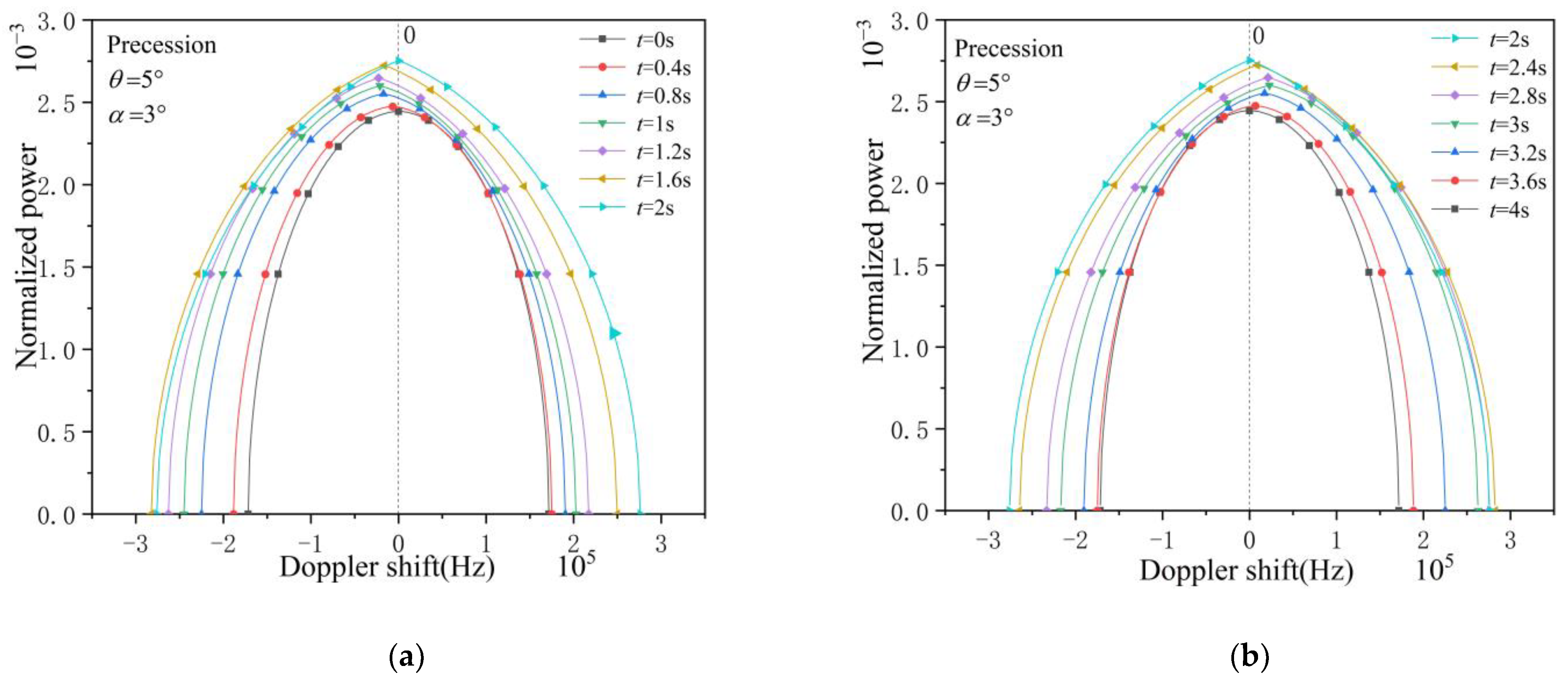
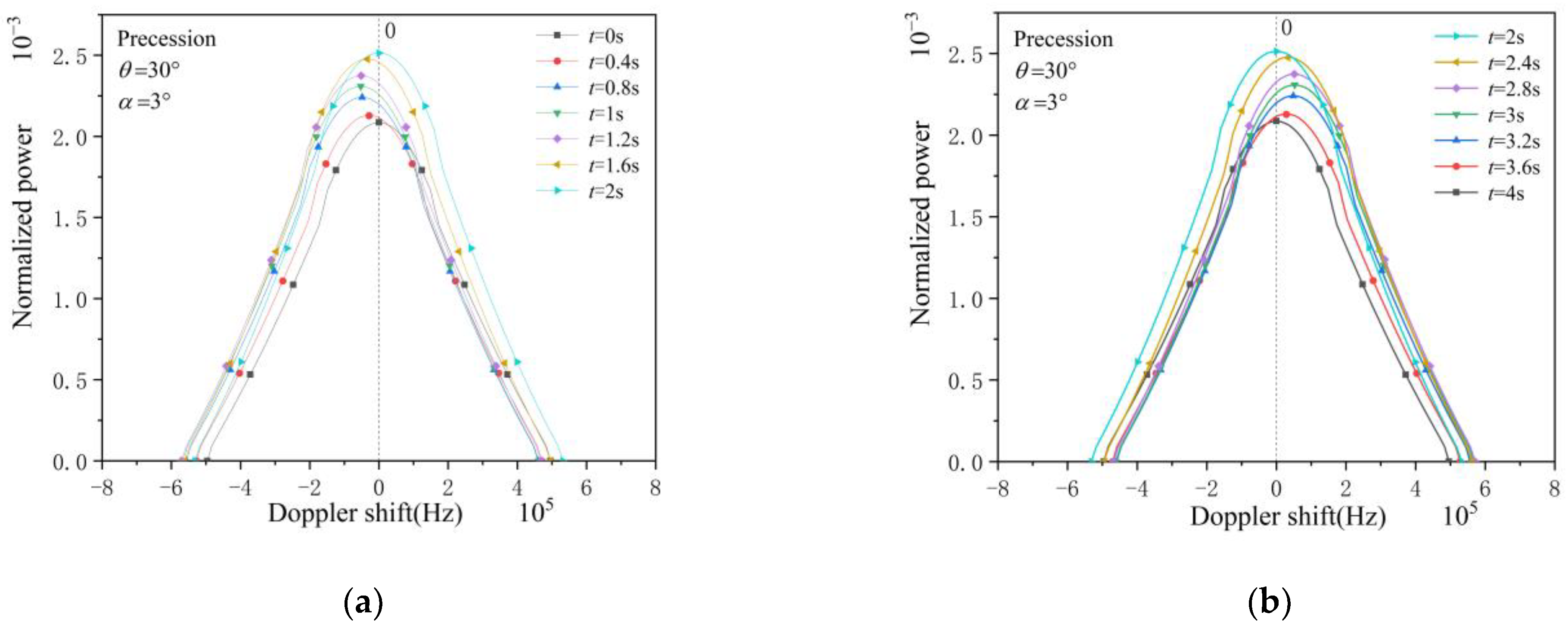
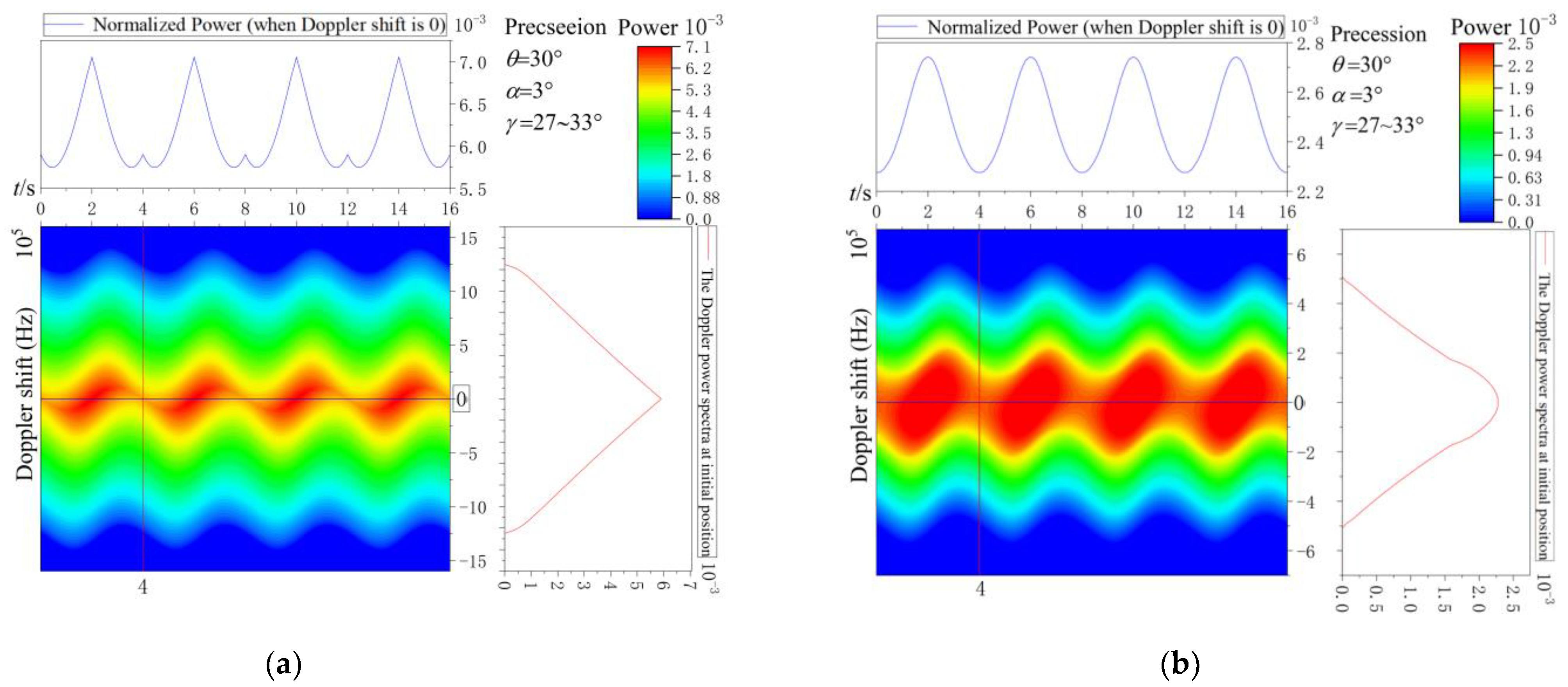
3.1. Precession Cone and Sphere–Cone Combination

For a cone, if $A={\tan }^2{\delta }_a,B=0,C=0$, the equation of the lateral surface of the convex quadric body of revolution is transformed as follows:

$$x^2+{(y\cos \gamma -z\sin \gamma )}^2={\tan }^2{\delta }_a{(y\sin \gamma +z\cos \gamma )}^2$$

(13)

where ${\delta }_a$ is the half-cone angle of the cone.

In a sphere–cone combination, the spherical and conical segments are joined to create a continuous slope on the surface.

$$\left[\begin{array}{c}A\\ B\\ C\end{array}\right]=\{\begin{array}{c}\left[\begin{array}{c}-1\\ r\\ 0\end{array}\right]\\ \left[\begin{array}{c}{\tan }^2{\delta }_b\\ r(\sec {\delta }_b-\tan {\delta }_b)\tan {\delta }_b\\ r^2{(\sec {\delta }_b-\tan {\delta }_b)}^2\end{array}\right]\end{array}\begin{array}{c}\begin{array}{c}\begin{array}{cc}& \\ ,& 0\le y\sin \gamma +z\cos \gamma <r(1-\sin {\delta }_b)\end{array}\\ \\ \begin{array}{cc}& \\ ,& r(1-\sin {\delta }_b)\le y\sin \gamma +z\cos \gamma \le h_b\end{array}\end{array}\\ \end{array}$$

(14)

The equation of the lateral surface of the convex quadric body of revolution is transformed as follows:

$$\begin{array}{l}{x}^2+{(y\cos \gamma -z\sin \gamma )}^2=\\ \{\begin{array}{ccc}-{(y\sin \gamma +z\cos \gamma )}^2+2r(y\sin \gamma +z\cos \gamma )& ,& 0\le y\sin \gamma +z\cos \gamma <r(1-\sin {\delta }_b)\\ & & \\ {(\tan {\delta }_b(y\sin \gamma +z\cos \gamma )+r\sec {\delta }_b-r\tan {\delta }_b)}^2& ,& r(1-\sin {\delta }_b)\le y\sin \gamma +z\cos \gamma \le h\end{array}\end{array}$$

(15)

where $r,{\delta }_b,h_b$ is the radius of the spherical segment, the half-cone angle of the conical segment, and the length. The base radius of the conical segment of the sphere–cone combination is $r_b$, where $r=\frac{r_b\cos {\delta }_b-h_b\sin {\delta }_b}{1-\sin {\delta }_b}$ (see Figure 2). We set simulation parameters for simulated computing spectra (see

Table 1. Simulation Parameters.

Parameters	Value
λ	1 μm
KL	1
ω	1 rad/s
ωp	0.5π rad/s
α	3°
ra	0.5 m
rb	0.2 m
ha	2 m
hb	1 m
δa	14.04°
δb	8°

).

Figure 3 is a schematic of the precession cone from position 1 to position 2, whose Doppler-normalized power spectrum is shown in Figure 4a. The normalized power is 10⁻³. With the increase in time $t$, both the Doppler shift and the normalized power increase due to the increase in the observation angle $\gamma$. Setting a reference line (dotted line) where the Doppler shift is equal to 0, we can find that the curves deviate to the left side of the dotted line except for at Position 1 and Position 2. Figure 4b shows the Doppler normalized power spectra from Position 2 to Position 1. Over time $t$, both the Doppler shift and the normalized power decrease due to the reduction in the observation angle $\gamma$. The curves deviate to the right side of the dotted line except for Position 1 and Position 2. Corresponding to the Doppler shift equation (Equation (4)), the Doppler shift is a function of x only at positions 1 and 2; at the other positions, the Doppler shift is a function of $x$ and $y$, which is reflected in the fact that the spectral lines will be skewed to the left and right of the dashed line.

Figure 5 illustrates that the Doppler power spectra for the combination of a sphere and a cone are dissimilar to those of the cone at lower frequencies, but comparable at higher frequencies. The simulated spectra of the sphere–cone combination enable the identification of composite features of the sphere and cone. Moreover, the normalized Doppler power spectra for the sphere–cone and cone during precession exhibit identical simulation outcomes.

The Doppler normalized power spectra of 0–4 s in Figure 4 and Figure 5 have been expanded to 0–16 s using a step size of $\mathsf{\Delta }t=0.1 \mathrm{s}$. The Doppler power spectra profiles for the precession cone and sphere–cone combination across four precession periods are illustrated in Figure 6. The upper blue curve illustrates the normalized power at a Doppler shift of zero. On the right, the red curve shows the Doppler power spectra of the cone during $t=4 \mathrm{s}$. In Figure 6, the Doppler power spectra profiles provide insight into the changes in Doppler frequency shift and normalized power across four precession periods, enabling a better understanding of target echo information during precession.

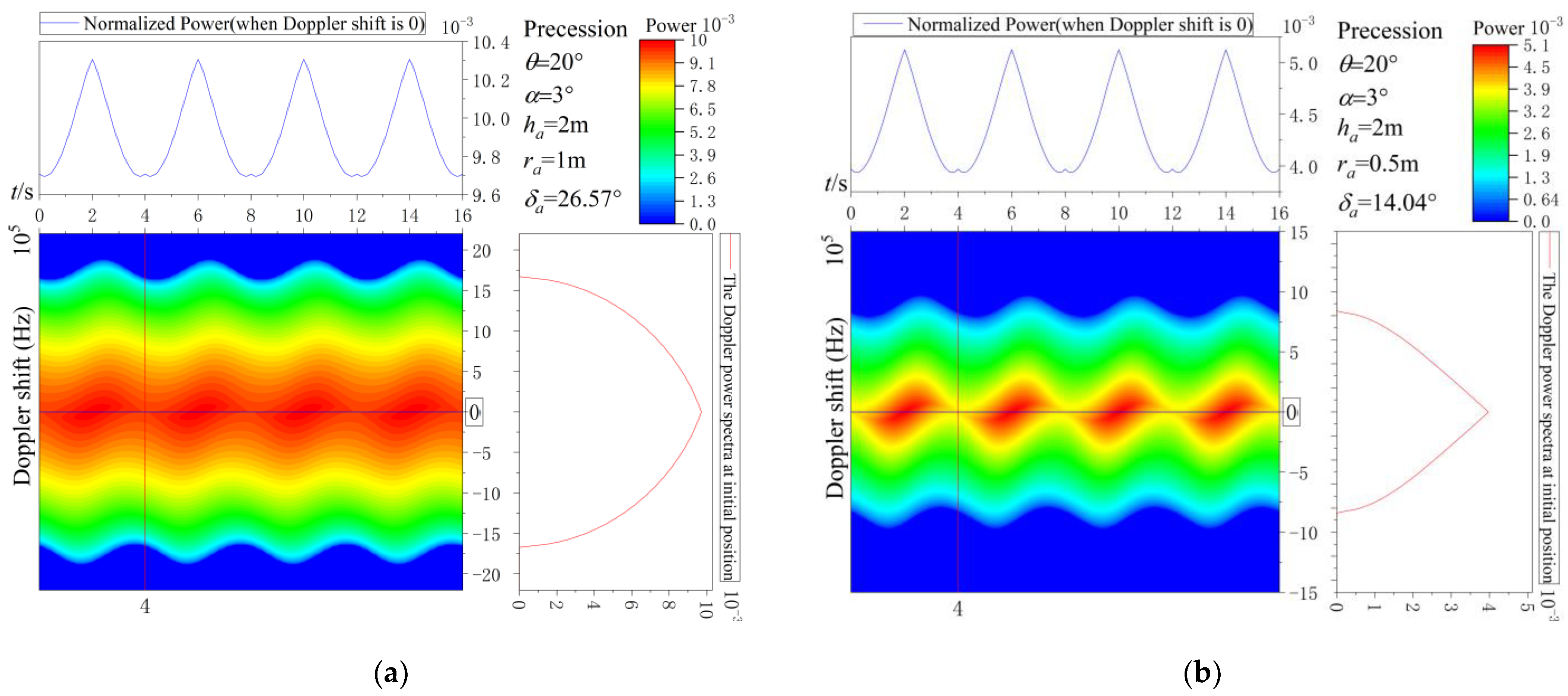
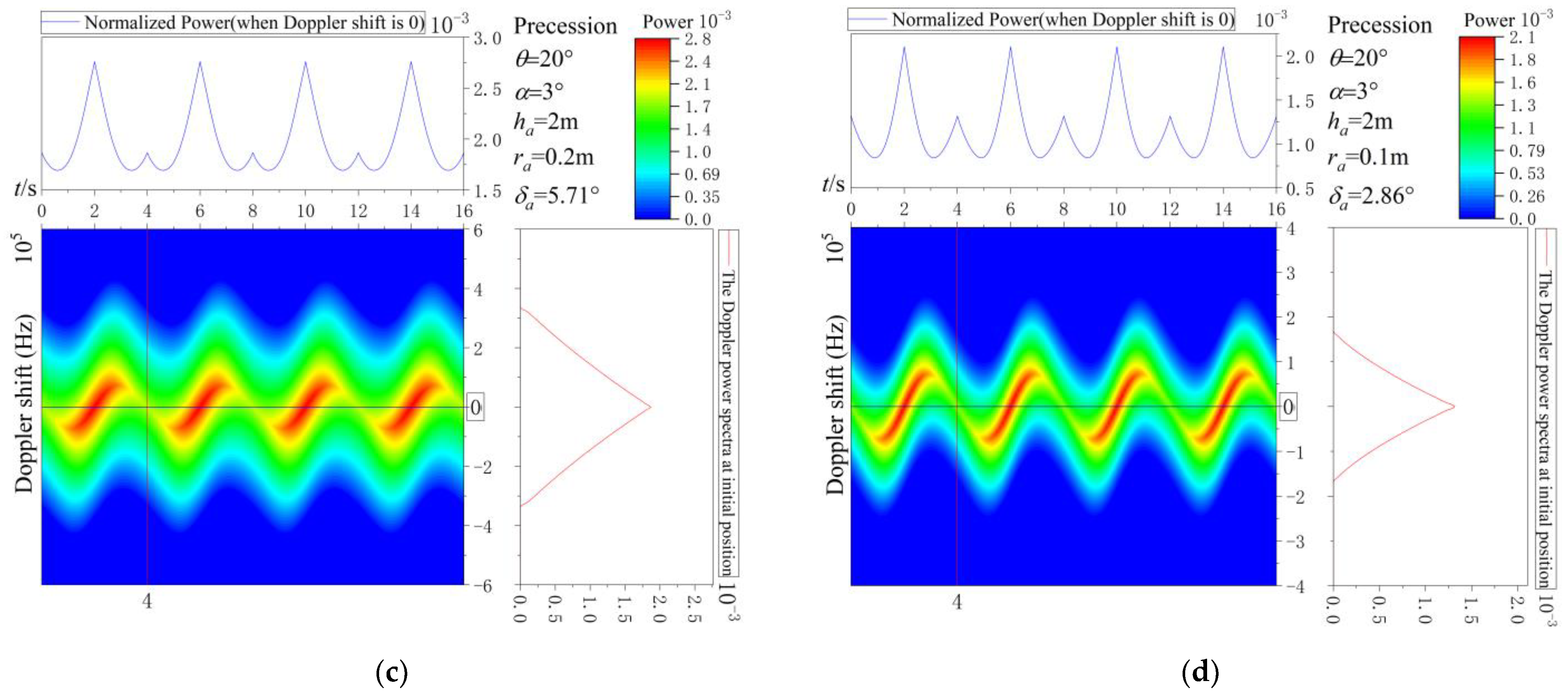
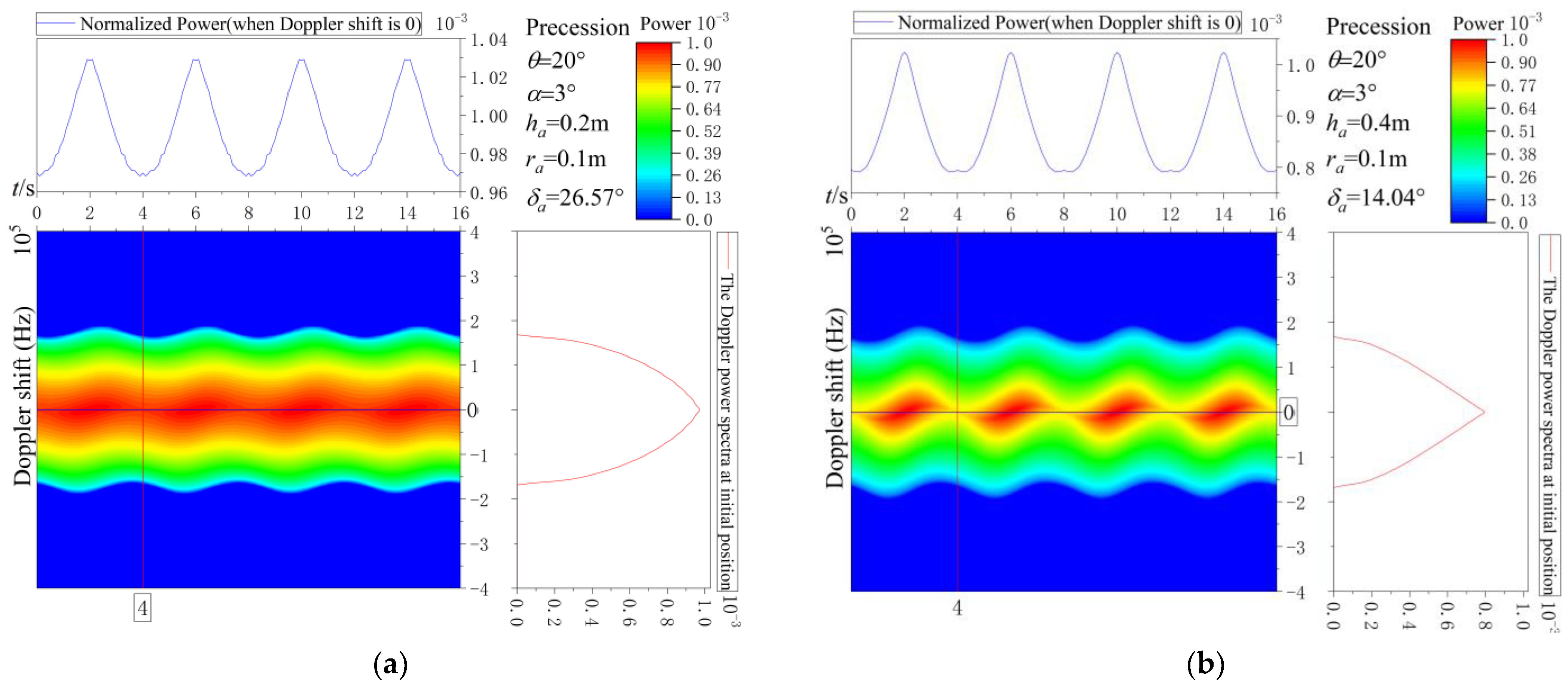
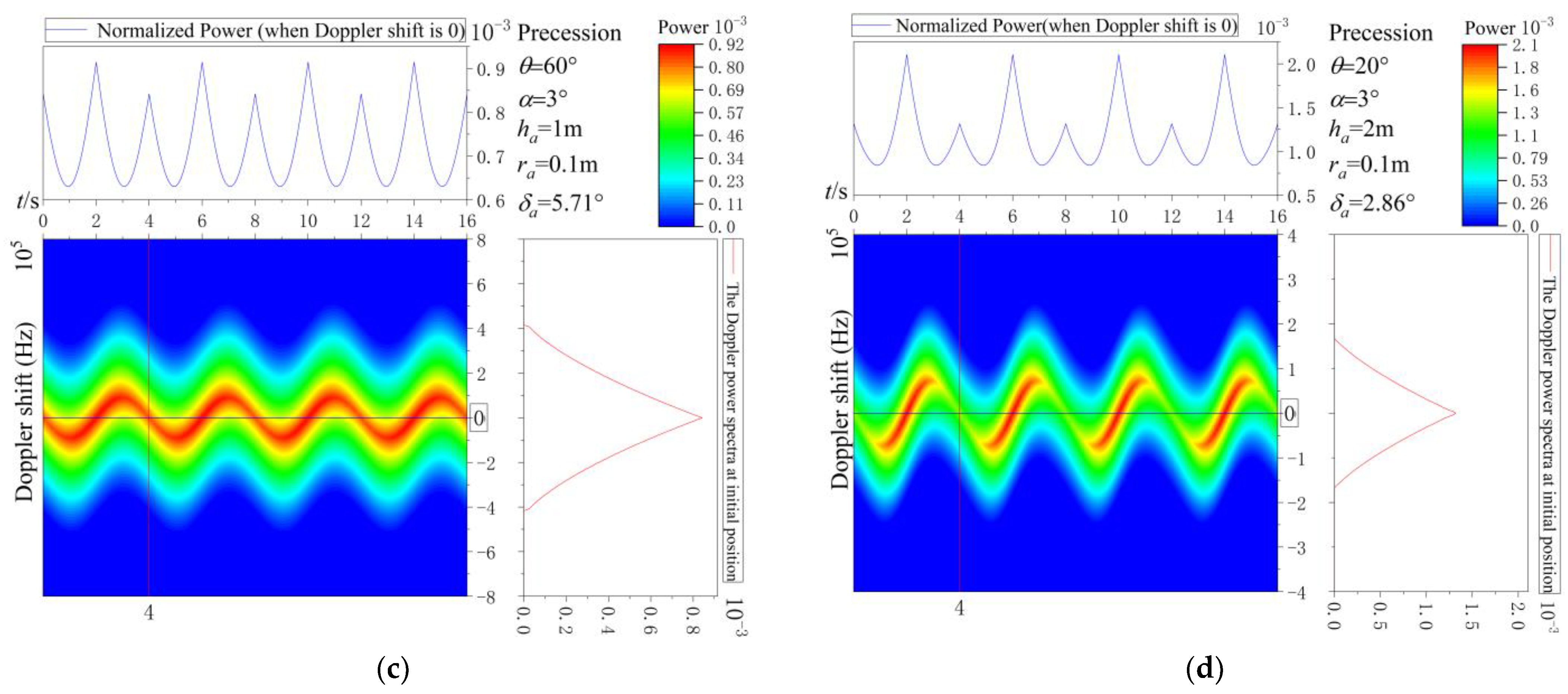
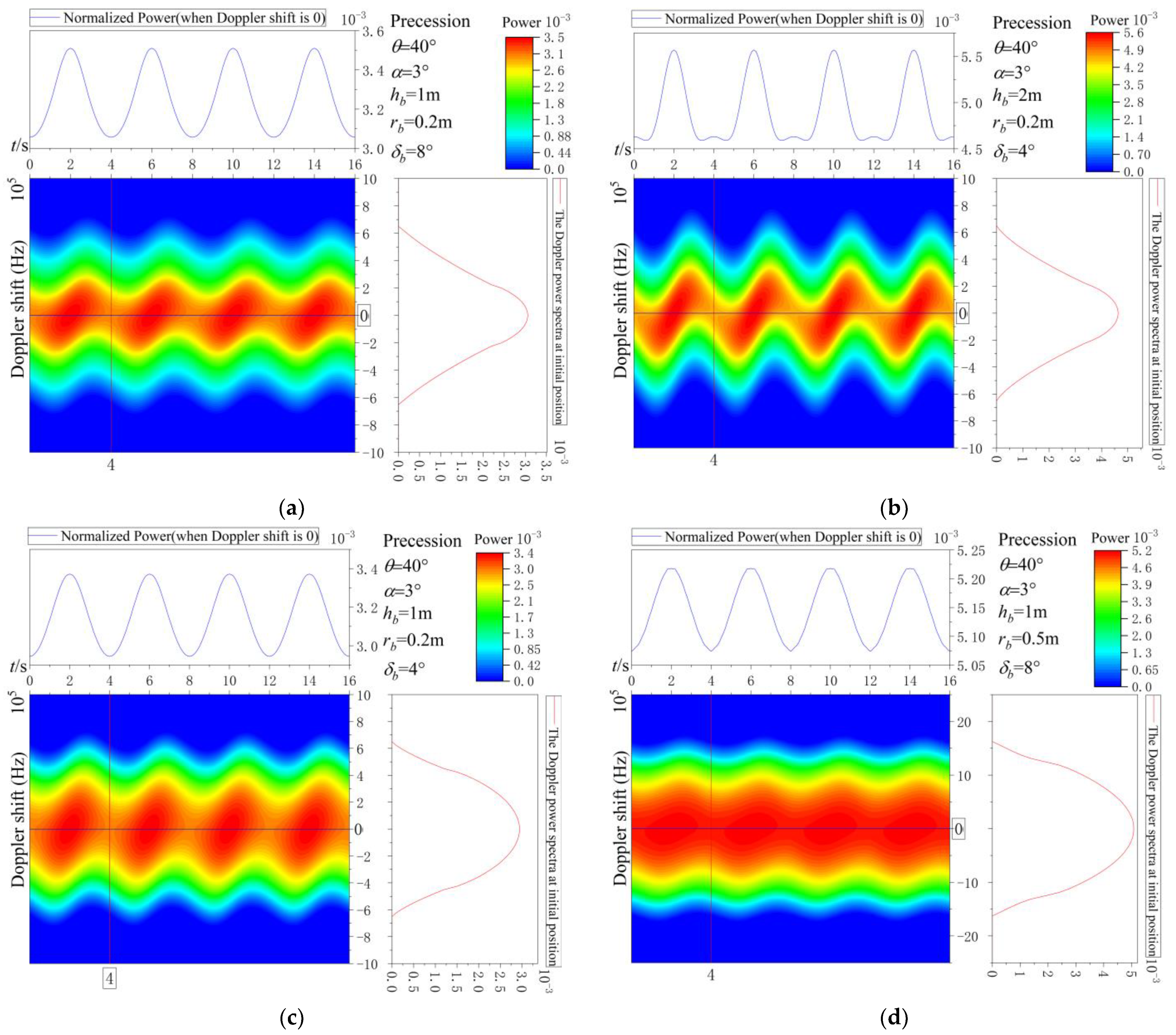
3.2. The Influence of Geometric Parameters on Doppler Spectra

Figure 7 shows the Doppler power spectra from 0 to 16 s in the precession process with a different radius of the cone. The blue curve on the top represents the normalized power when the Doppler shift equals 0. The red curve on the right represents the Doppler power spectra of the cone when $t=4\mathrm{s}$. We found that the geometric parameters of the cone affect the Doppler power spectra.

As the radius of the cone decreases, the Doppler shift decreases. This result is the same as the Doppler shift formula Equation (5) we analyzed.

The change in radius affects the area of the target irradiated surface. The larger the radius is, the larger the surface irradiated area is, and the larger the normalized power value of the obtained image is.

Figure 8 shows the Doppler power spectra from 0 to 16 s in the precession process with different heights of the cone. The blue curve on the top represents the normalized power when the Doppler shift equals 0. The red curve on the right represents the Doppler power spectra of the cone when $t=4\mathrm{s}$. We found that the geometric parameters of the cone affect the Doppler power spectra.

When the radius remains constant, there is no change in the Doppler shift width of the obtained Doppler spectra. Similarly, altering the height does not affect the Doppler shift width.

As the height of the cone in Figure 7a–d increases, the normalized power value increases, which is because the irradiated area of the target surface increases as the height increases.

When studying the change in geometric parameters of the sphere–cone combination, the radius of the sphere at the blunt head is given by:

$$r=\frac{r_b\cos {\delta }_b-h_b\sin {\delta }_b}{1-\sin {\delta }_b}$$

The radii of the spheres of Figure 9a–d are 0.0684, 0.0645, 0.1395, and 0.4135. It can be analyzed from the aforementioned figures that:

(1) Figure 9a,c depict the Doppler power spectra profile of the sphere–cone combination with an 8° and 4° cone half-angle, respectively, and the sphere radius of 0.0684 and 0.1395. An enlarged spherical radius yields a more extensive area exposed to low frequencies, which, in turn, results in an increase in normalized power. The Doppler shift width remains unchanged as the base radius remains constant.

(2) Figure 9b,c display the Doppler power spectra of the sphere–cone combination at a height of 2 m and 1 m for a sphere radius of 0.0645 and 0.1395, respectively. As the base radius remains constant, there is no alteration in the Doppler shift width. It can be inferred that the Doppler shift width remains the same, while the power at the center of the low frequency increases.

(3) Figure 9a,d show Doppler power spectra profiles for a sphere–cone combination with base radii of 0.2 m and 0.5 m, respectively, and a sphere radius of 0.0684 and 0.4135. The change in base radius affects the spherical radius, resulting in differences in the spectra in terms of both power at low frequency and Doppler shift width. An increased base radius widens the spectral lines.

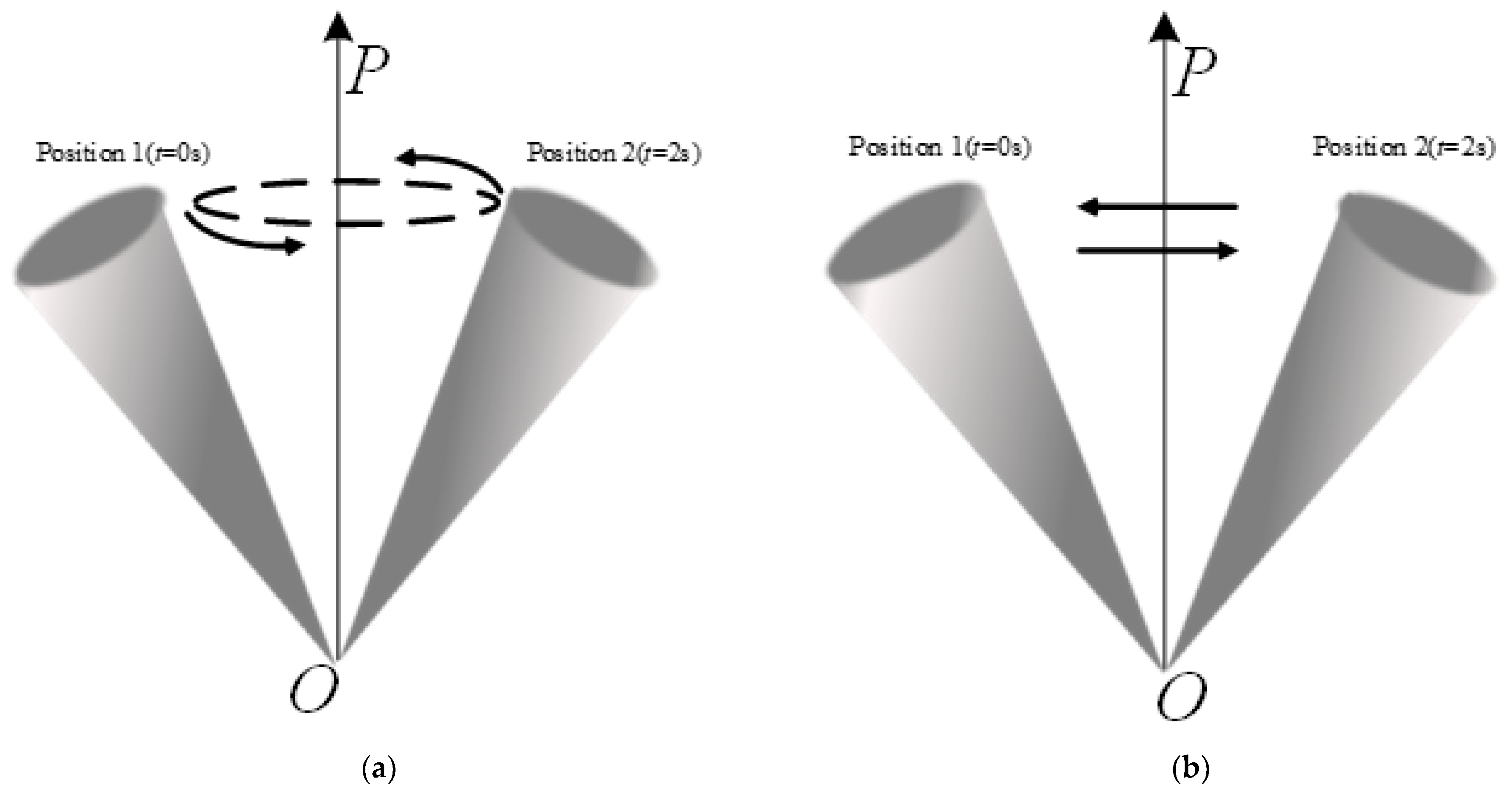
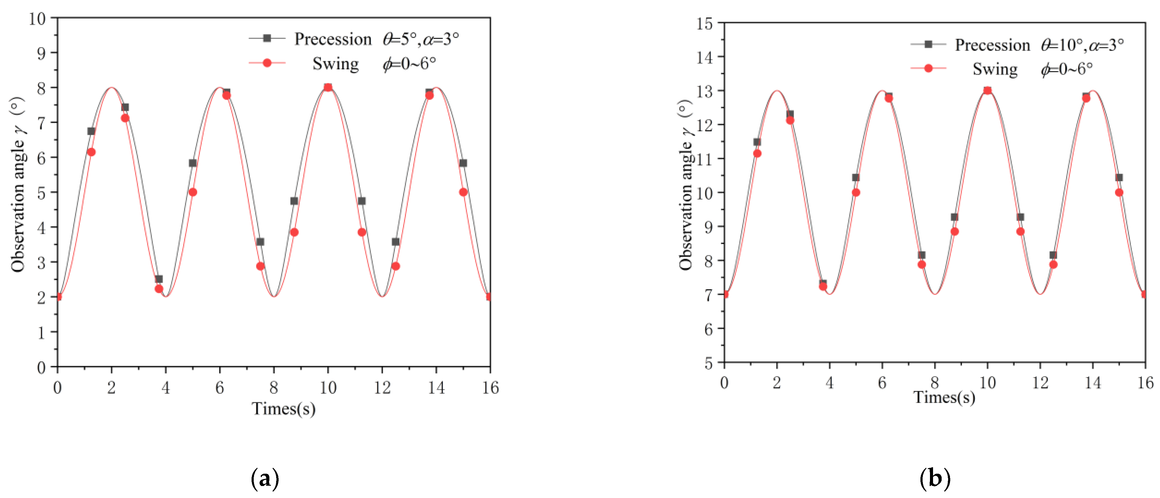
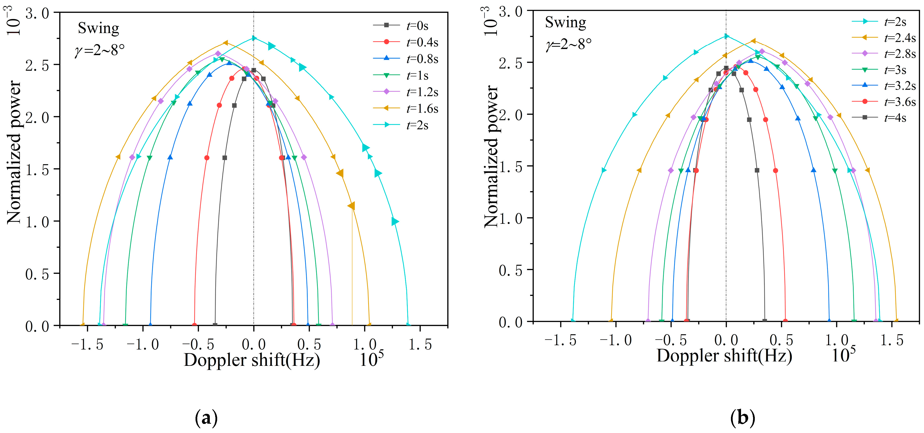
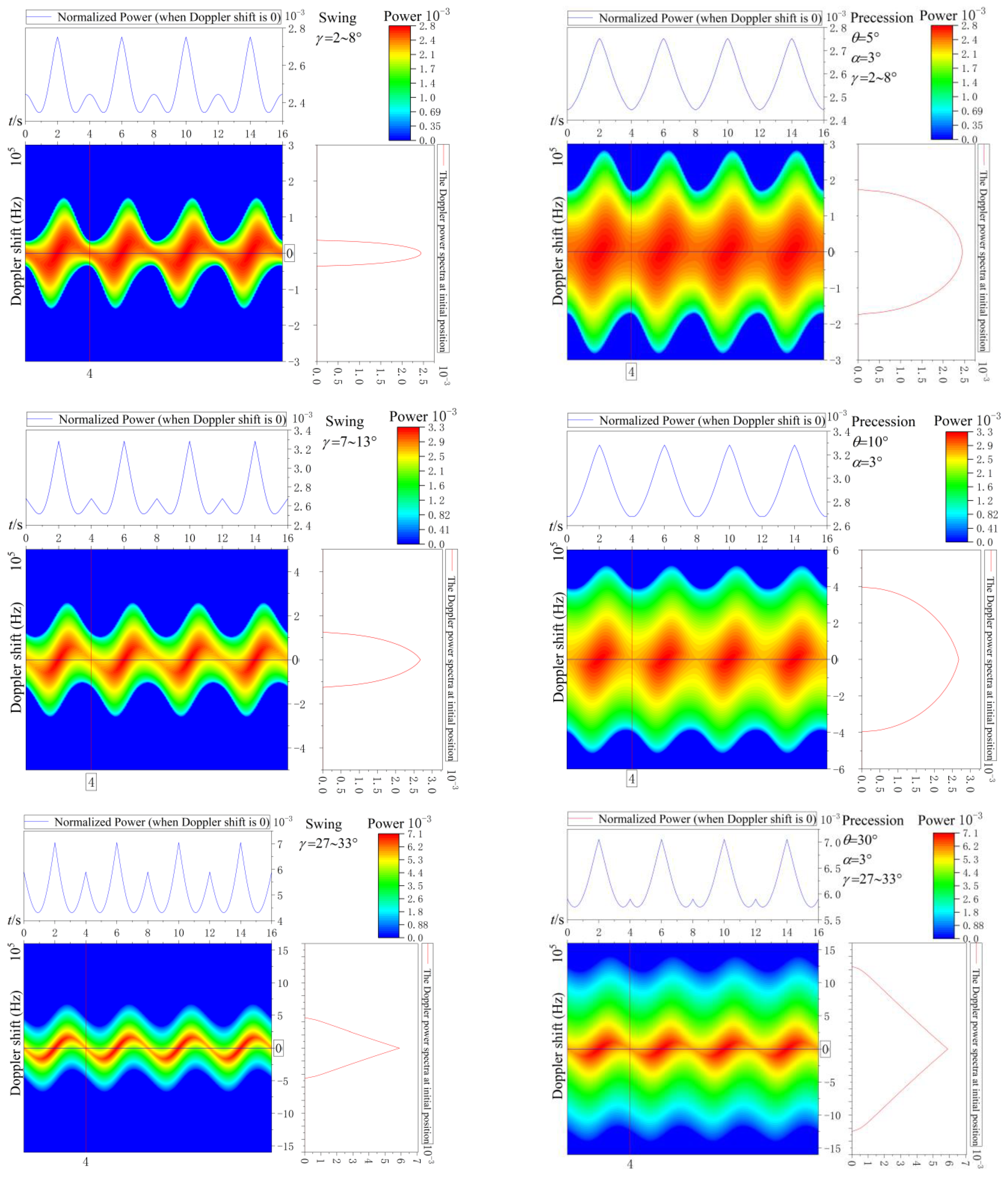
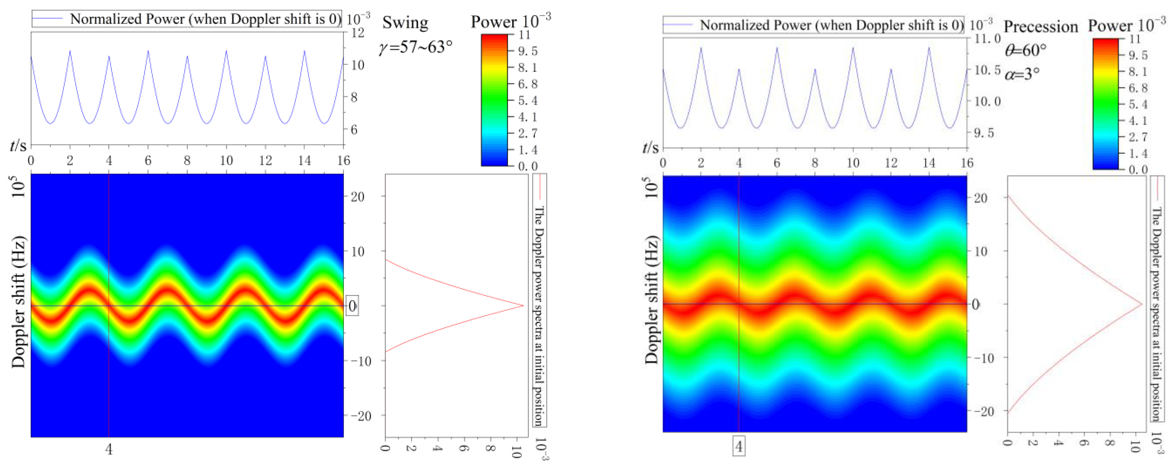
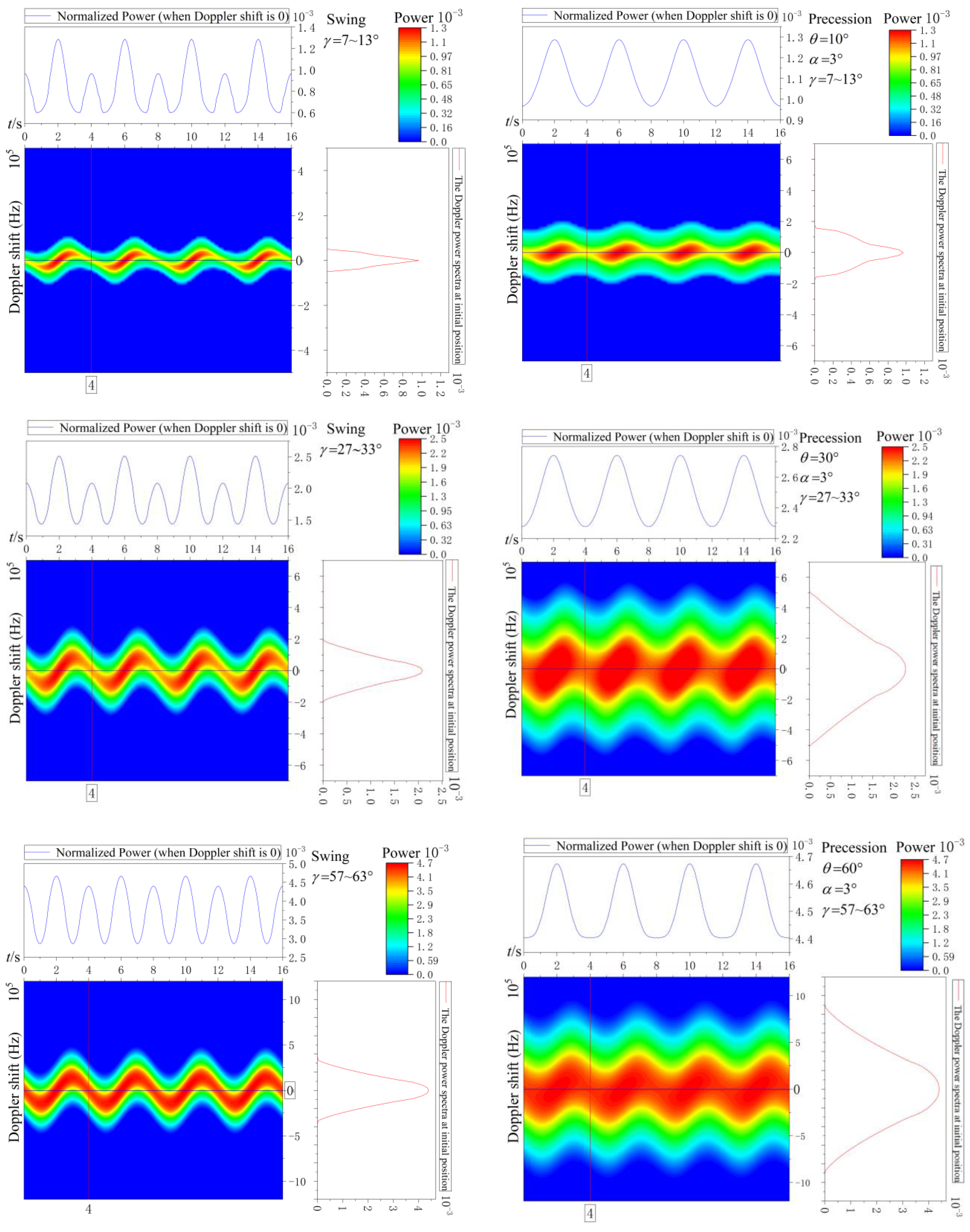
3.3. Precession Cone and Swing Cone

Swing and precession are common forms of micro-motion for spatial targets, characterized by periodic changes in the observation angle; however, their paths of micro-motion diverge. In order to differentiate the Doppler power spectra for various micro-motion forms, we analyzed the swing cone and compared it with the precession cone in this model. In Figure 10, Figure 10a illustrates the concept of precession, depicted as a cone executing a rotational movement around a central axis. Figure 10b demonstrates the principle of swing, where the cone undergoes motion around its apex, confined to a single plane.

The convex quadric body of revolution spins around its central axis $\stackrel{\rightharpoonup }{OT}$ with angular velocity $\omega$ while $\stackrel{\rightharpoonup }{OT}$ swings in the $yoz$ plane. Swing angle $\varphi$:

$$\varphi ={\varphi }_1\sin ({\omega }_n\cdot t+{\psi }_1)+{\varphi }_2$$

(16)

where ${\varphi }_1$ is the amplitude of swing angle, ${\omega }_n=\frac{2\pi }{T_n}$ ($T_n$ is the swing period), ${\psi }_1$ is the initial swing phase angle, and ${\varphi }_2$ is the initial swing angle. The axis of symmetry of the cone can be given by:

$$\stackrel{\rightharpoonup }{O{T}^{″}}=(0,\sin (\theta -\alpha +\varphi ),\cos (\theta -\alpha +\varphi ))$$

(17)

Spinning around $\stackrel{\rightharpoonup }{O{T}^{″}}$: For each point $r(x,y,z)$ on the lateral surface, the vector of angular velocity can be expressed as ${\stackrel{\rightharpoonup }{\Omega }}_{\mathit{spin}}=\omega \cdot (0,\sin (\theta -\alpha +\varphi ),\cos (\theta -\alpha +\varphi ))$, while its linear velocity ${\stackrel{\rightharpoonup }{v}}_{\mathit{spin}}$ is given by:

$$\begin{array}{ll}{\stackrel{\rightharpoonup }{v}}_{\mathit{spin}}& ={\stackrel{\rightharpoonup }{\Omega }}_{spin}\times \overrightarrow{r}\\ & =\omega \cdot (0,\sin (\theta -\alpha +\varphi ),\cos (\theta -\alpha +\varphi ))\times (x,y,z)\\ & =\omega \cdot (z\sin (\theta -\alpha +\varphi )-y\cos (\theta -\alpha +\varphi ),x\cos (\theta -\alpha +\varphi ),-x\sin (\theta -\alpha +\varphi ))\end{array}$$

(18)

When the target swings, the vector of angular velocity can be expressed as ${\stackrel{\rightharpoonup }{\Omega }}_{\mathit{swing}}=\frac{d\varphi }{dt}\cdot (1,0,0)$, and its linear velocity ${\stackrel{\rightharpoonup }{v}}_{swing}$ is given by:

$$\begin{array}{ll}{\stackrel{\rightharpoonup }{v}}_{swing}& ={\stackrel{\rightharpoonup }{\Omega }}_{swing}\times \overrightarrow{r}\\ & =\frac{d\varphi }{dt}\cdot (1,0,0)\times (x,y,z)\\ & ={\omega }_n{\varphi }_1\cos ({\omega }_n\cdot t+{\psi }_1)\cdot (0,-z,y)\end{array}$$

(19)

So, the linear velocity of micro-motion of the cone can be measured by $\stackrel{\rightharpoonup }{v}$:

$$\stackrel{\rightharpoonup }{v}={\stackrel{\rightharpoonup }{v}}_{swing}+{\stackrel{\rightharpoonup }{v}}_{spin}$$

(20)

The incidence direction of the laser can be expressed as $\stackrel{\rightharpoonup }{e}=(0,0,1)$, the Doppler shift for any point on the surface of the cone, if the direction of backscattering is as follows:

$$\begin{array}{ll}\mathsf{\Delta }f& =-\frac{2(\stackrel{\rightharpoonup }{v}\cdot \stackrel{\rightharpoonup }{e})}{\lambda }\\ & =\frac{2\omega x\sin (\theta -\alpha +\varphi )}{\lambda }-\frac{2{\omega }_n{\varphi }_1\cos ({\omega }_n\cdot t+{\psi }_1)y}{\lambda }\end{array}$$

(21)

Simulation parameters for the swing are presented in

Table 2. Simulation Parameters of swing.

Parameters	Value
Tn	4 s
ϕ1	3°
Ψ1	−0.5π rad/s
ϕ2	3°

, where the swing angle is denoted by $0\le \varphi \le 6°$. The remaining parameters hold identical values to those in Table 1.

The observation angle in the swing can be written as follows:

$$\gamma =\theta -\alpha +\varphi$$

(22)

The range of angles for observing the two micro-motion forms can be expressed as

$$\theta -3°\le \gamma \le \theta +3°.$$

(23)

Figure 11 illustrates that precession and swing correspond only at Position 1 and Position 2 with regards to the observation angle $\gamma$ (refer to Figure 10). The varying forms of micro-motion result in a dissimilar route between the two positions.

Figure 12 shows the Doppler normalized power spectra for the swing cone. From Figure 4 and Figure 12, we can clearly find:

At Positions 1 and 2, the value of normalized power for the precession cone and swing cone are the maximum when the Doppler shift is equal to 0. From Equations (5) and (21), the Doppler shift $\mathsf{\Delta }f$ is only a function of $\mathrm{x}$ when $t=0,2,4\dots \mathrm{s}$, and the curves are symmetrical about the dotted line. When $t\ne 0,2,4\dots \mathrm{s}$, the Doppler shift $\mathsf{\Delta }f$ is a function of $x$ and $y$, and the curves deviate left or right side of the dotted line.

With the same range of variation in $\gamma$, the Doppler shift of the precession cone is greater than that of the swing cone. However, their normalized power sizes are almost equal.

Figure 13 shows the Doppler power spectra from 0 to 16 s in the swing process and precession process with the variation range of $\gamma$ increased. For precession and swing, the range of $\gamma$ varying from $2\sim 8°$ to $57\sim 63°$ produces the red curves with increasing width and height. From the blue curves, multiple factors can be observed.

For the identical range of variation in $\gamma$, the blue curves show distinct tendencies in precession and swing, with greater prominence at small angles.

For the swing, the minimum is indicated by the blue curves when $t=1,3,5,7,9,11,13,15s$ is at its maximum and $t=2,6,10,14s$ is at its minimum (Position 2). For precession, if $\gamma =2\sim 8°,7\sim 13°$, the blue curves are the minimum when $t=0,4,8,12,16s$ (Position 1), and it is the maximum when $t=2,6,10,14s$ (Position 2). With the increase in the observation angle $\gamma$, the minimum value occurs somewhere on the path between Positions 1 and 2. When $\gamma =57\sim 63°$, it is the minimum when $t=1,3,5,7,9,11,13,15s$.

For the identical range of variation in $\gamma$, the normalized power of precession and swing display nearly identical magnitudes. However, the minimum of the blue curves in precession is greater than in swing. This outcome is consistent with the deviation magnitude of the curves presented in Figure 4 and Figure 12.

Figure 14 illustrates the Doppler power spectra of the sphere–cone configuration during both the swing and precession processes, with a variation range of $\gamma$, recorded between 0 and 16 s. The sphere–cone combination and cone target exhibit comparable simulated outcomes, except for the blue curves during precession. The potential reasons for this outcome are that:

(1) The spectral difference at low frequencies between the cone and sphere–cone combination is being examined.

(2) The deflection of the curve in Figure 6 while undergoing precession is lower than that seen in Figure 12.

This demonstrates the effectiveness of our analytical model for complex targets and its potential to differentiate between target shape and micro-movement.

4. Conclusions

This paper presents an analytical model for rotating convex tetrahedra to simulate two special cases, namely, the combination of a cone and a sphere–cone. Based on this model, the Doppler power spectra for oscillating conical objects, oscillating sphere–cone combinations, forward-scattering conical objects, and forward-scattering sphere–cone combinations are analyzed. In simulations, we observed that geometric parameters only affect the magnitude of the received signal power and the Doppler frequency shift, while the temporal trends in the spectra remain unchanged. Changes in target profile affect the Doppler spectra, but do not affect the trend of Doppler spectra during the approach, and individual spectra can reflect target profile information. When other parameters are held constant, the Doppler shift broadens and the normalized power increases when the angle of view is increased. The variation in the base radius affects the size of the targetable surface area, which in turn influences the magnitude of the echo power. Specifically, a larger radius results in a larger illuminable surface area, leading to higher normalized power values in the obtained images. However, this does not affect the overall trend in the precession spectrum. Different micro-motion forms, such as forward tilt and oscillation, exhibit nearly identical received signal power within the same range of observation angles. However, the differences in Doppler frequency shifts result in distinct Doppler power spectra. This paper solely analyzes the Doppler power spectra for various targets and micro-motion forms. In practical applications, factors such as target surface roughness, atmospheric scattering, absorption, and turbulence effects on laser beams should also be considered.

References

1. Verly, J.G.; Delanoy, R.L. Model-based automatic target recognition (ATR) system for forward-looking ground based and airborne imaging laser radars (LIDAR). Proc. IEEE 1996, 84, 126–163. [Google Scholar] [CrossRef]
2. Jelalian, A.V. Laser Radar Systems; Artech House: Boston, MA, USA, 1992. [Google Scholar]
3. Pearson, G.; Davies, F.; Collier, C. Remote Sensing of the Tropical Rain Forest Boundary Layer Using Pulsed Doppler Lidar. Atmos. Chem. Phys. 2010, 10, 5891–5901. [Google Scholar] [CrossRef]
4. Kollias, P.; Rémillard, J.; Luke, E.; Szyrmer, W. Cloud Radar Doppler Spectra in Drizzling Stratiform Clouds: 1. Forward Modeling and Remote Sensing Applications. J. Geophys. Res. 2011, 116, D13201. [Google Scholar] [CrossRef]
5. Chen, V.C. Analysis of radar micro-Doppler with time-frequency transform. In Proceedings of the Tenth IEEE Workshop on Statistical Signal and Array Processing (Cat. No.00TH8496), Pocono Manor, PA, USA, 16 August 2000. [Google Scholar]
6. Chen, V.C. The Micro-Doppler Effect in Radar; Artech House: Boston, MA, USA, 2011. [Google Scholar]
7. Yura, H.T.; Hanson, S.G.; Lading, L. Laser doppler velocimetry: Analytical solution to the optical system including the effects of partial coherence of the target. J. Opt. Soc. Am. A 1995, 12, 2040–2047. [Google Scholar] [CrossRef]
8. Youmans, D.G. Cylindrical target Doppler and Doppler-spread feature estimation using coherent mode-locked pulse laser radars with long observation times. Proc. SPIE Int. Soc. Opt. Eng. 2001, 4377, 272–283. [Google Scholar]
9. Bankman, I.N. Model of laser radar signatures of ballistic missile warheads. Proc. SPIE Int. Soc. Opt. Eng. 1999, 3699, 133–137. [Google Scholar]
10. Gong, Y.; Wu, Z.; Wang, M.; Cao, Y. Laser backscattering analytical model of Doppler power spectra about rotating convex quadric bodies of revolution. Opt. Lasers Eng. 2010, 48, 107–113. [Google Scholar] [CrossRef]
11. Manninen, A.J.; Marke, T.; Tuononen, M.J.; O’Connor, E.J. Atmospheric boundary layer classification with Doppler lidar. J. Geophys. Res. Atmos. 2018, 123, 8172–8189. [Google Scholar] [CrossRef]
12. Peng, X.; Shan, J. Detection and Tracking of Pedestrians Using Doppler LiDAR. Remote Sens. 2021, 13, 2952. [Google Scholar] [CrossRef]
13. Bankman, I. Analytical model of Doppler spectra of coherent light backscattered from rotating cone and cylinders. J. Opt. Soc. Am. Opt. Image Sci. Vis. 2000, 17, 465–476. [Google Scholar] [CrossRef] [PubMed]
14. Liu, L.; McLernon, D.; Ghogho, M.; Hu, W.; Huang, J. Ballistic missile detection via micro-Doppler frequency estimation from radar return. Digit. Signal Process. 2012, 22, 87–95. [Google Scholar] [CrossRef]
15. Gao, H.; Xie, L.; Wen, S.; Kuang, Y. Micro-Doppler Signature Extraction from Ballistic Target with Micro-Motions. Aerosp. Electron. Syst. IEEE Trans. 2010, 46, 1969–1982. [Google Scholar] [CrossRef]
16. Chen, V.C. Doppler signatures of radar backscattering from objects with micro-motions. IET Signal Process. 2008, 2, 291–300. [Google Scholar] [CrossRef]
17. Han, X.; Du, L.; Liu, H.W.; Shao, C.Y. Classification of micro-motion form of space cone-shaped objects based on time-frequency distribution. Syst. Eng. Electron. 2013, 35, 684–691. [Google Scholar]
18. Wang, N.; Mo, D.; Song, Z.; Wang, R.; Wu, Y. Feature extraction algorithm of a precession target based on a Doppler frequency profile of dual-aspect observation. Appl. Opt. 2019, 58, 4695–4700. [Google Scholar] [CrossRef] [PubMed]
19. Zhang, Q.; Hu, J.; Luo, Y.; Chen, Y. Research progresses in radar feature extraction, imaging, and recognition of target with micro-motions. J. Radars 2018, 7, 531–547. [Google Scholar] [CrossRef]
Figure 1. Schematic diagram of a convex quadrilateral rotating body.
Remotesensing 16 01104 g001
Figure 2. Schematic diagrams of cones (a) and blunt tapers (b).
Remotesensing 16 01104 g002
Figure 3. Schematic diagrams of precession.
Remotesensing 16 01104 g003
Figure 4. The Doppler normalized power spectra for the precession cone (a) position 1 to position 2 and (b) position 2 to position 1.
Remotesensing 16 01104 g004
Figure 5. The Doppler normalized power spectra for the precession sphere–cone combination (a) position 1 to position 2 and (b) position 2 to position 1.
Remotesensing 16 01104 g005
Figure 6. The normalized power spectra profile for the Doppler precession cone (a) and sphere–cone (b) combination within 0~16 s.
Remotesensing 16 01104 g006
Figure 7. The Doppler power spectra profile for the precession cone ( h a = 2   m , r a = (a) 1 m, (b) 0.5 m, (c) 0.2 m, (d) 0.1 m) within 0~16 s.
Remotesensing 16 01104 g007aRemotesensing 16 01104 g007b
Figure 8. The Doppler power spectra profile for the precession cone ( r a = 0.1   m , h a = (a) 0.2 m, (b) 0.4 m, (c) 1 m, (d) 2 m) within 0~16 s.
Remotesensing 16 01104 g008aRemotesensing 16 01104 g008b
Figure 9. The Doppler power spectra profile for the precession sphere–cone combination within 0~16 s.
Remotesensing 16 01104 g009
Figure 10. Schematic diagrams of precession (a) and swing (b).
Remotesensing 16 01104 g010
Figure 11. Observation angle sequence in (a) precession and (b) swing.
Remotesensing 16 01104 g011
Figure 12. The Doppler normalized power spectra for the swing cone (a) position 1 and (b) position 2.
Remotesensing 16 01104 g012
Figure 13. The Doppler power spectra profile for the precession cone and the swing cone.
Remotesensing 16 01104 g013aRemotesensing 16 01104 g013b
Figure 14. The Doppler power spectra profile for the sphere–cone combination.
Remotesensing 16 01104 g014