


Airborne Short-Baseline Millimeter Wave InSAR System Analysis and Experimental Results
by
 ,
,
Luhao Wang
1,2,
Yabo Liu
1,*,
Qingxin Chen
1,
Xiaojie Zhou
3,
Shuang Zhu
1,2 and
Shilong Chen
1,2 
1
Aerospace Information Research Institute, Chinese Academy of Sciences, Beijing 100094, China
2
School of Electronic, Electrical and Communication Engineering, University of Chinese Academy of Sciences, Beijing 100049, China
3
School of Electronic Information Engineering, University of Beihang, Beijing 100083, China
*
Author to whom correspondence should be addressed.
Remote Sens. 2024, 16(6), 1020; https://doi.org/10.3390/rs16061020
Submission received: 6 February 2024
/
Revised: 8 March 2024
/
Accepted: 11 March 2024
/
Published: 13 March 2024
(This article belongs to the Special Issue Imaging Geodesy and Infrastructure Monitoring II)
Abstract
:For the challenges of high-precision mapping in complex terrain, a novel airborne Interferometric Synthetic Aperture Radar (InSAR) system is designed. This system, named ASMIS (Airborne Short-Baseline Millimeter-Wave InSAR System), adopts the coplanar antenna and a pod-type structure. This design makes the system lightweight and highly integrated. It can be compatible with small general aviation flight platforms. The baseline is millimeters in size, which greatly simplifies the unwrapping process. The coplanar antennas have two advantages: they maximize the baseline utilization and minimize the Doppler decorrelation and the motion error inconsistency. Acquisition campaigns of the system have been carried out in Boao, Bayannur, and Chengde, China. In the Chengde experimental area, we designed an antiparallel flight experiment to account for the topographic relief. High-precision Digital Orthophoto Maps (DOMs) and Digital Surface Models (DSMs) at a scale of 1:5000 were obtained. The coordinate Root Mean Square Error (RMSE) of the checkpoints within the obtained DSM is less than 0.82 m in altitude and 3 m horizontally. The RMSE of the Sparse Ground Control Points (GCPs) within the obtained DSM is less than 0.3 m in altitude. Experimental results from different areas, including plains, mountains, and coastlines, demonstrate the system’s performance.
1. Introduction
InSAR is widely used for high-precision Digital Elevation Models (DEMs) of the ground, which are utilized in various applications such as topographic mapping, glacier monitoring, disaster monitoring, and deformation estimation [1,2,3,4,5,6].
Satellites and airplanes are the primary carriers of InSAR systems. Different orbital models give spaceborne and airborne systems distinct advantages. Spaceborne systems are suitable for obtaining global DEMs because of the orbit geometry. In 1994, Zebker [7] analytically validated the generation of DEMs from ERS-1 repeat orbit data in Alaska and the western U.S., with relative accuracies of less than 5 m in localized areas. In 1998, Rufino et al. [8] used a DEM generated from ERS-1 TanDEM model data to obtain GCPs elevation accuracies at about 4 m, with elevation accuracies of 20 m. The TanDEM-X satellite, launched by Deutsches Zentrum für Luft- und Raumfahrt (DLR) in 2010, adopts a star formation flight mode and can achieve an elevation coverage area of 150 million square kilometers with an absolute spatial resolution of 12 m, a relative elevation accuracy of 2 m, an absolute elevation accuracy of 4 m, and a revisit period of 11 days [9,10]. The C-band GF-3 satellite, launched by China in 2016, can perform global observation and imaging with a 500 km swath using the across-track interferometry (XTI) mode. It has an elevation accuracy of 2.9 m in Guangdong, China, and a revisit period of 4 days [11]. Existing spaceborne systems generally use interferometric measurements in the X-band and lower bands with a mapping accuracy of 1:50,000 for DOM and DSM. This is more suitable for global large-scale mapping. However, the spaceborne system faces some technical difficulties, such as limited orbit geometry, launch power, and attitude-orbit control [12]. The spaceborne system generally adopts the formation of XTI or Repeat Orbit Interferometry (RTI), which leads to baseline and temporal decorrelation due to the longer baseline and revisit period [13,14,15]. The inconsistent motion error of the interferometry antennas introduces additional phase error, requiring complex processing algorithms [16,17,18]. The small look angle of high-orbit characteristics results in the layover of complex terrain areas, which affects the accuracy of surveying and mapping. Additionally, the revisit period is longer, which means a mission cannot be completed quickly [19,20].
Airborne systems are more flexible and can quickly respond to work requirements. The use of millimeter-wave transmitting signals, such as Ka and W, along with dual-antenna XTI, is an important direction for the development of high-precision topographic mapping [21,22]. Fixing antennas on the airplane ensures the feasibility of acquiring multi-scene images in a single pass. It can improve baseline measurement accuracy, reduce the effects of temporal decorrelation and atmospheric decorrelation, and improve elevation accuracy. Some of the typical airborne systems include GeoSAR, a dual antenna system that uses multiple bands and was developed jointly by the National Aeronautics and Space Administration (NASA) and Jet Propulsion Laboratory (JPL). The system is positioned under a single wing and has a baseline of 20 m/2.5 m (P/X-band). It is particularly useful for mapping the vegetation canopy with high accuracy [23]. Pi-SAR2, an X-band system developed by the National Institute of Information and Communications (NICT) of Japan, mounted on both sides of the fuselage, with a baseline length of 2.6 m for disaster emergency monitoring, achieved 2 m elevation accuracy [24]. Dual-antenna X-band InSAR developed by East China Research Institute of Electronic Enginery (ECRIEE), China, with a baseline length of 1.7 m, used for topographic mapping in western China, achieved an elevation accuracy of 2–5 m [25]. The Institute of Electrics, Chinese Academy of Sciences (IECAS) developed the first Chinese airborne millimeter-wave triple-baseline InSAR principle prototype in 2011. The triple baseline adopted a separate structure, with a spatial resolution of 0.5 m and an elevation accuracy of 1 m [26]. Airborne systems are flexible, making them more suitable for monitoring rapidly changing geologic hazards, such as earthquakes, volcanoes, and landslides [27,28,29]. However, the airborne platform is greatly affected by airflow, resulting in technical difficulties with flight attitude and trajectory, as well as obvious Doppler decorrelation. When the baseline is too long, the flexible baseline problem should be appreciated. Since the individual antenna has limited application, it requires customization and design to suit the carrier structure and maintain airworthiness. This is not ideal for small general aviation flight platforms because the platform has strict requirements for compliance.
In this work, we present a novel airborne short-baseline millimeter-wave InSAR system. The system has several important characteristics. Firstly, the antenna has been designed with an integrated pod-type structure and is strategically placed on the symmetry axis at the center of the airplane. This provides exceptional stability and makes it easy to install on a variety of small general aviation flight platforms, including the Harbin Y-12 and the Cessna 208. Secondly, the short baseline avoids the flexible baseline problem and simplifies the interferometric phase unwrapping algorithm [30,31,32]. Thirdly, the design of a dual-channel coplanar antenna allows for precise control of distance and angle between the antennas. It can maximize baseline utilization and avoid the influence of the vertical component of the baseline. In addition, the attitude of antennas is consistent, which helps to improve the inconsistency of the doppler decorrelation and motion error. It reduces the difficulty of motion compensation and registration. The proposed system is designed to be used in complex terrain and for high-precision mapping scenarios, as outlined in Table 1.
The main research work of this paper includes: the advantages of the pod-type structure are analyzed by comparing different antenna installation forms, and the baseline is designed according to safety requirements. The theoretical basis for ASMIS elevation accuracy and coherence is obtained by analyzing sensitivity and motion error. After completing the system performance analysis, we describe the system structure composition in detail, as well as the functions and indispensability of each module. We designed different flight routes according to the experimental area’s terrain characteristics.
In 2022 and 2023, flight experiments were conducted in Boao, Bayannur, and Chengde, China, covering different terrain and features such as fields, plains, coastal zones, and mountains. While experimenting, the flight platform was affected by the troposphere, causing some of the flight data to be acquired under non-steady conditions. This accounts for approximately 10% of the data. After processing the flight data, we were able to obtain high-precision DOM and DSM standard products at a scale of 1:5000.
The work is organized as follows: Section 2 analyzes the baseline design and error; Section 3 briefly describes the structure and parameters of the system; Section 4 covers the flight experiment and data processing; Section 5 describes the experiment results and elevation accuracy analysis; finally, Section 6 reports the discussion and conclusion.
2. Design and Analysis
2.1. Baseline Design
2.1.1. Antenna Mount Analysis
In a dual-antenna airborne system, a long interferometric baseline can cause elastic deformation and instability, leading to large differences in antenna phases. This is known as the flexible baseline and has no standard reference value, as it depends on platform parameters [32]. External influence disrupts motion trajectory, making motion estimation and compensation challenging. Design stability is crucial for performance analysis and data processing.
The installation of XTI airborne systems is divided into separate and integrated types. The separate type includes single and double wings, as shown in Figure 1a. Different methods of antenna installation have varying impacts on systems. The separate type can improve the sensitivity of the interferometric phase and help generate a high-precision DEM. However, the flexible baseline effect may cause issues with motion compensation and result in geometric phase error. The integrated type (Figure 1b) is relatively stable, and the antennas share the same attitude. The use of a lever arm in connecting antennas can lead to the flexible baseline effect, which increases motion error. However, this issue is eliminated in the integrated design since the antennas are not connected through the lever arm. This design is suitable for various small general aviation flight platforms. Nonetheless, obtaining a high-precision DEM with a short baseline can be challenging, but it can be solved through baseline angle design and algorithm processing [31].
To achieve accurate mapping, ASMIS utilizes a pod-type mounting design with integrated antennas. Two millimeter-wave antennas in a single pod with a short baseline and coplanar configuration ensure consistent geometry for interferometric images.
2.1.2. Baseline Length Limit
The antenna installation envelope design must account for the safe ground clearance when the system is under the carrier’s center of gravity during loading, take-off, and landing. Figure 2 shows the installation and design dimensions of the antenna system’s outer envelope for normal platform operation. The example uses Y-12 and Cessna 208 with safety distances of 210 mm and 250 mm respectively.
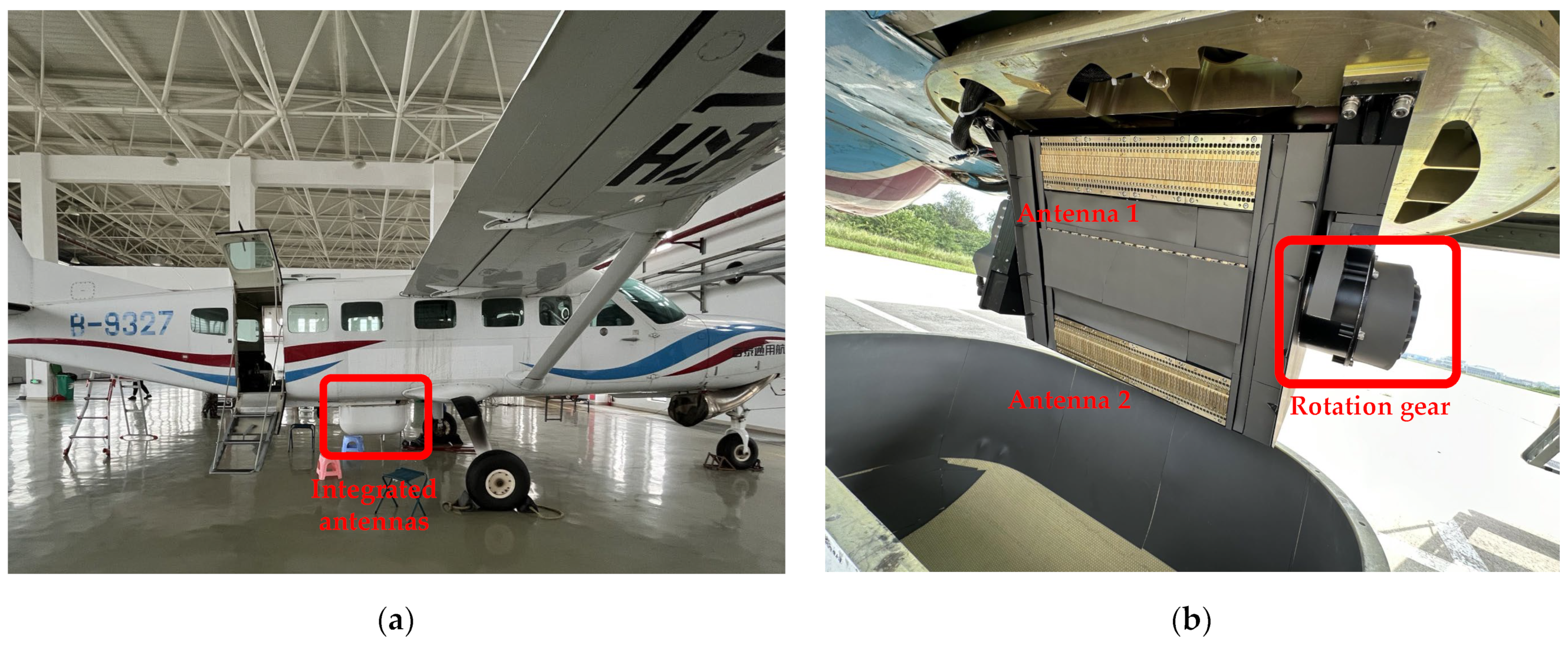
Special safety considerations are taken into account for the departure angle due to the placement of the Cessna optical window behind the rear wheel. To ensure the safe installation of the antenna unit, the center of gravity is shifted forward by 263 mm towards the nose. In Figure 2a, this design places the antenna installation envelope within the baggage compartment envelope. In addition, to provide adjustment within a certain range of baseline angle, a rotating mechanism is added during antenna integration (see Figure 3b), thus ensuring the utilization rate of the baseline. Based on this, considering the safety and the normal operation of the rotating mechanism, the maximum length of the design baseline is 0.32 m. Figure 3a is the installation of ASMIS. The pod-type antenna is mounted at the center of gravity under the Cessna 208. The details of the antenna structure are shown in Figure 3b.
Before the flight experiment, we analyze the system’s performance using a short baseline and the coplanar antenna design characteristics. We focus on elevation accuracy, coherence indicators, and providing reference performance indicators for ASMIS and system parameters. The simulation data used are derived from real data from laboratory or flight experiments.
2.2. Elevation Error
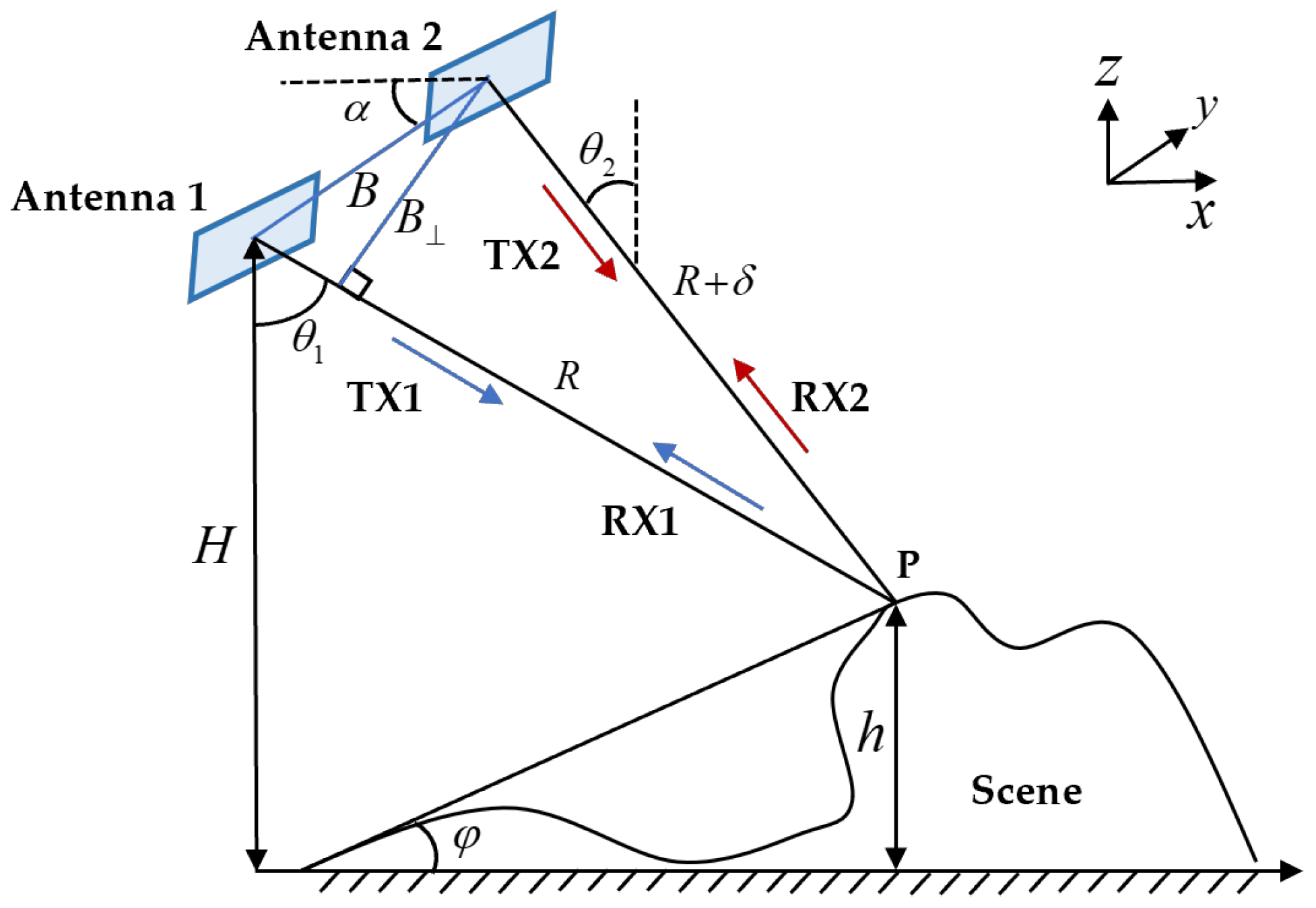
It is important to quantitatively analyze and evaluate various error sources that affect elevation accuracy measurements. This analysis helps in selecting appropriate InSAR system parameters, such as baseline length, work altitude, radar parameters, and look angle. The imaging geometry of ASMIS is illustrated in Figure 4. The system employs a ping-pong mode, where two antennas use time-sharing to alternately transmit and receive their respective signals. According to the interferometry principle and the geometric relationship, the elevation of the ground point P can be obtained by Equation (1) [33]:
where is the relative altitude of antenna 1, is the look angle of antenna 1, is the distance from antenna 1 to point P, is the baseline angle, is the difference in distance from the antennas to point P, and is the baseline length. There is a relationship in the InSAR system: , . Therefore, the approximate relationship can be taken as: .
In Equation (1), the error terms affecting the accuracy of elevation measurement are mainly the flight altitude, range, baseline angle, baseline length, and interferometric phase error. The baseline utilization is 100% when satisfied , which can be achieved by rotating the mechanism (Figure 3b). When calculating the relative error at the same work altitude, the system’s flight altitude error can be compensated by the Inertial Measurement Unit (IMU) data. The item can be disregarded when analyzing the elevation accuracy. Then, according to Equation (1), by calculating the differential coefficients, the relationship between the error source and the elevation error can be obtained by Equation (2) [34]:
where is the interferometric phase. Table 2 gives the system parameters of ASMIS and the accuracies used as a quantitative analysis of elevation error and coherence.
According to the law of covariance propagation, assuming that these error sources are independent of each other, the elevation error can be obtained by Equation (3):
where and , , , , and are slant error, baseline angle error, interferometric phase error, baseline length error, and look angle error, respectively. is the correlation coefficient. and are the azimuth and range multi-look numbers, respectively.
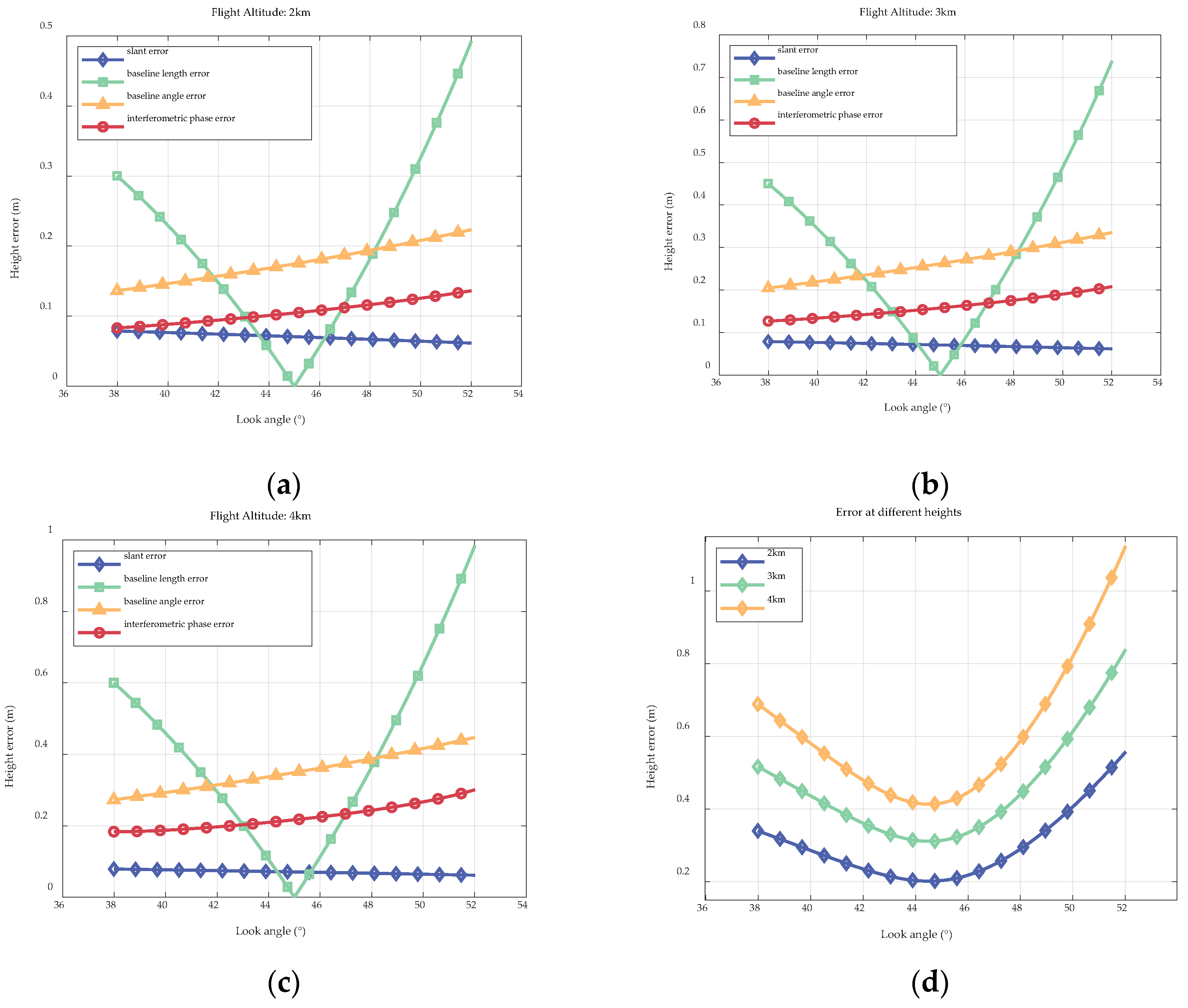
The relative elevation errors due to each error are given in Figure 5a–c for typical flight altitudes of 2 km, 3 km, and 4 km, respectively. The x-axis of the graph is the range of look angle (36°–54°) and the y-axis is the elevation error. Comparative analysis shows that the elevation errors due to baseline length error and baseline look error are greatly affected by the slant range, and reducing the platform flight altitude will narrow these two errors. As the flight altitude decreases, it will increase the elevation accuracy error due to the interferometric phase error. The variation of elevation error with look angle at different altitudes is shown in Figure 5d.
As shown in Figure 5, the elevation error rises with the flight altitude. The baseline angle error at the scene center is the most significant, while the baseline length error is the least. Considering the effect of flight error, it is recommended that the relative use altitude of the XTI mode is 4000 m and below to get better elevation accuracy. The elevation error of the irradiated scene is usually less than 0.4 m, satisfying the 1:5000 high-precision mapping requirement. Using the scene center as the reference, the far- and near-end elevation data can be externally calibrated for higher elevation accuracy.
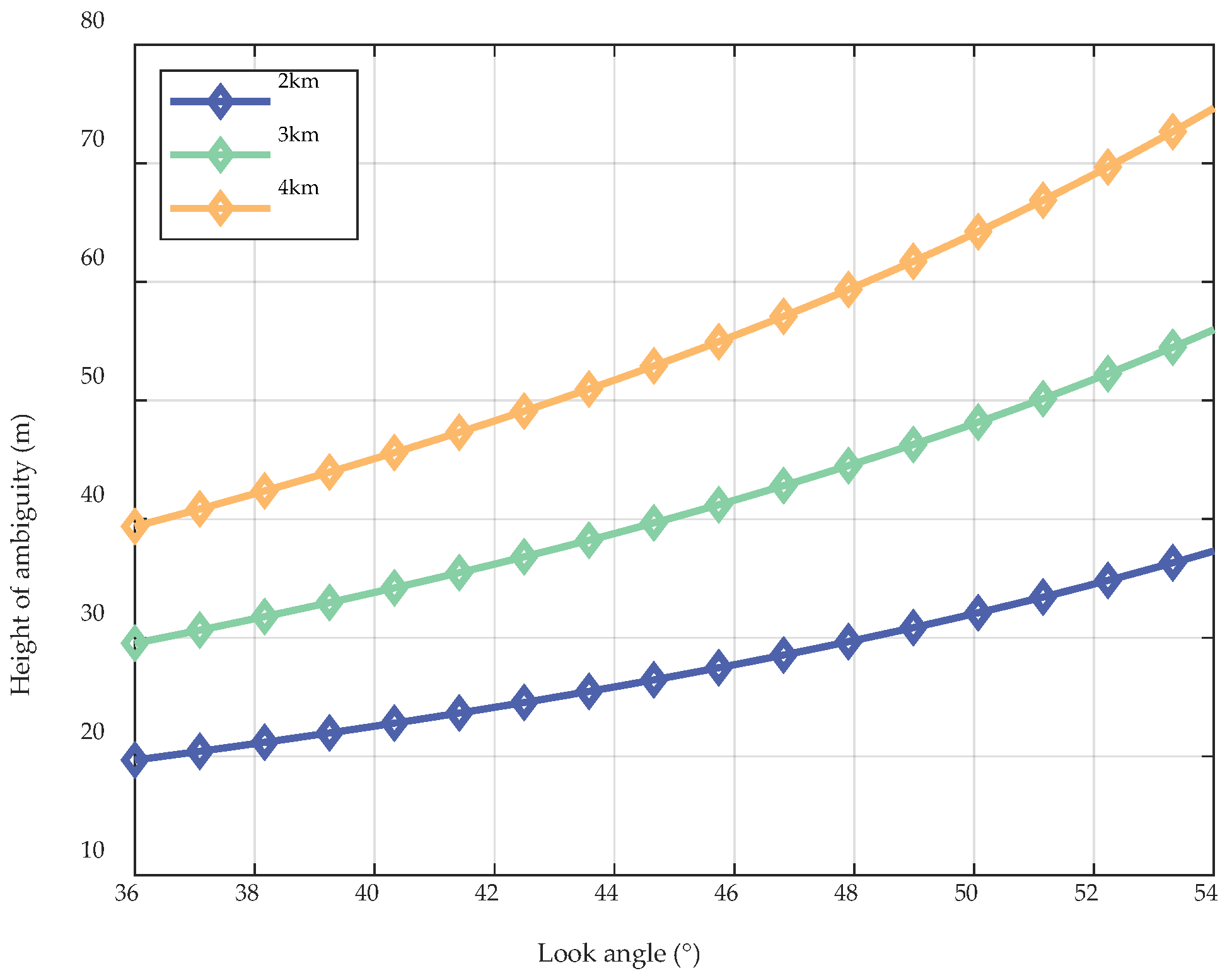
In Equation (2), the altitude change corresponding to a phase change caused by interferometric phase error is the cause of elevation ambiguity , which can be obtained by Equation (4):
Figure 6 shows the variations in elevation ambiguity with look angle and altitude. The experimental results in Figure 5 confirm that ASMIS has no elevation ambiguity at different altitudes within the elevation error range. A short baseline results in high coherence, greater sensitivity to terrain altitude variations, and higher accuracy during interferometry and phase unwrapping, without elevation ambiguity.
According to the results in Figure 5d, when the flight altitude is 4 km, the elevation error is 0.4136 m at the look angle of 45°. The small elevation error results in small azimuth and range offsets and negligible azimuth variation residual error on the planar positioning. This enables the system to achieve the 1:5000 mapping theoretically [35].
2.3. Coherence
The analysis in Section 2.2 shows that the interference phase accuracy is the key factor for the elevation accuracy, other than the system measurement error. The effect of interferometric phase accuracy on image phase information also dominates. There are two main factors affecting the interferometric phase accuracy: random phase errors due to various decorrelation factors and fixed phase errors introduced by inaccuracies in motion compensation. The phase error caused by the decorrelation is usually reduced by phase filtering to improve the coherence. The interferometric phase error introduced by the motion error is complex, and different interferometric systems are affected differently to some extent. The corresponding compensation means should be analyzed before interferometry processing to ensure accuracy.
2.3.1. Decorrelation
There are numerous sources of random errors affecting the coherence, and the decorrelation is reflected in the interferometric phase that affects the performance and the measurement accuracy. In addition to external factor errors, the effects of decorrelation arising from system design include baseline decorrelation , Doppler decorrelation , and thermal noise decorrelation . The effect of short baseline and coplanar antenna design on the decorrelation of the ASMIS is analyzed in the following.
- Baseline Decorrelation
When using XTI to observe the same surface area with a short baseline, the backscattering coefficients of the targets within the area are considered the same. However, as the baseline length increases, the dual antenna’s orbital geometry becomes more different, and the backward scattering coefficients within the same resolution cell are no longer approximately equal, causing baseline decorrelation. The echo spectrum causes a ground distance band offset from the look angle deviation of the two antennas in the interferogram formation. Interferometric preprocessing eliminates the spectral offset, as only the same ground range band has coherent information. For systems with a defined bandwidth and carrier frequency, according to the spectral shift theory of F. Gatelli [36], there is a limit to the baseline length of the interferometric system, which can be obtained by Equation (5):
where is the range resolution. Equation (5) shows that when the spectral shift of a two-channel InSAR exceeds the system bandwidth , it loses coherence and can no longer interferometric processing. Accordingly, under the condition of , we can obtain the baseline decorrelation by Equation (6):
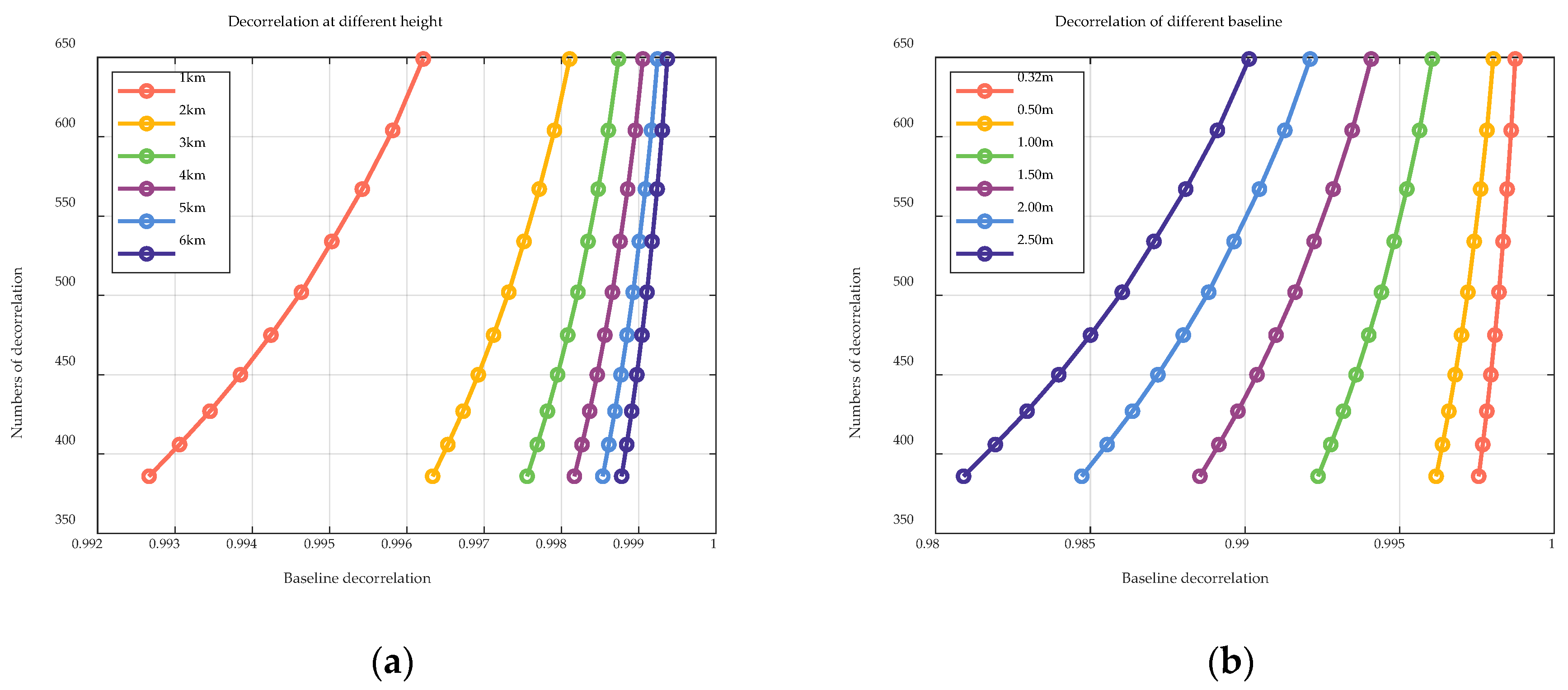
In Equation (6), the baseline decorrelation is affected by the combination of baseline length, resolution, wavelength, slant range, and look angle. In a certain look angle, Equation (6) illustrates that the baseline decorrelation is inversely proportional to the baseline length and directly proportional to the flight altitude. The baseline decorrelation for the range of look angles at different altitudes is shown in Figure 7. The x-axis in the figure is the range of baseline decorrelation, and the y-axis is the numbers in each range. From Figure 7, the short baseline design leads to a very high decorrelation, which makes the effect of baseline decorrelation on the coherence of the interferometric image pairs almost negligible.
- 2.
- Doppler Decorrelation
Similarly to baseline decorrelation, doppler decorrelation is caused by the inconsistency of the doppler center frequencies of the interferometric image in azimuth, which will decrease linearly with the increase of the doppler center frequency difference irrespective of the directional map weighted of the spectra [37,38]. can be obtained by Equation (7):
where is the Doppler center frequency difference. is the azimuth bandwidth. Regarding the ASMIS, it can be assumed that the doppler decorrelation factor is zero. This is because the phase centers of the two antennas are the same in the azimuthal direction, and the structure of the co-array surface exhibits the same form of dual-antenna error when subjected to external perturbations.
- 3.
- Thermal Noise Decorrelation
is the result of random thermal noise generated by the electronic components of the radar system, which affects the accuracy and stability of the interferometric phase and can be improved by filtering. For dual-channel InSAR, assuming that the thermal noise of the channels is incoherent and the transmit signal is incoherent with the noise, the thermal noise decorrelation can be calculated by Equation (8) [38]:
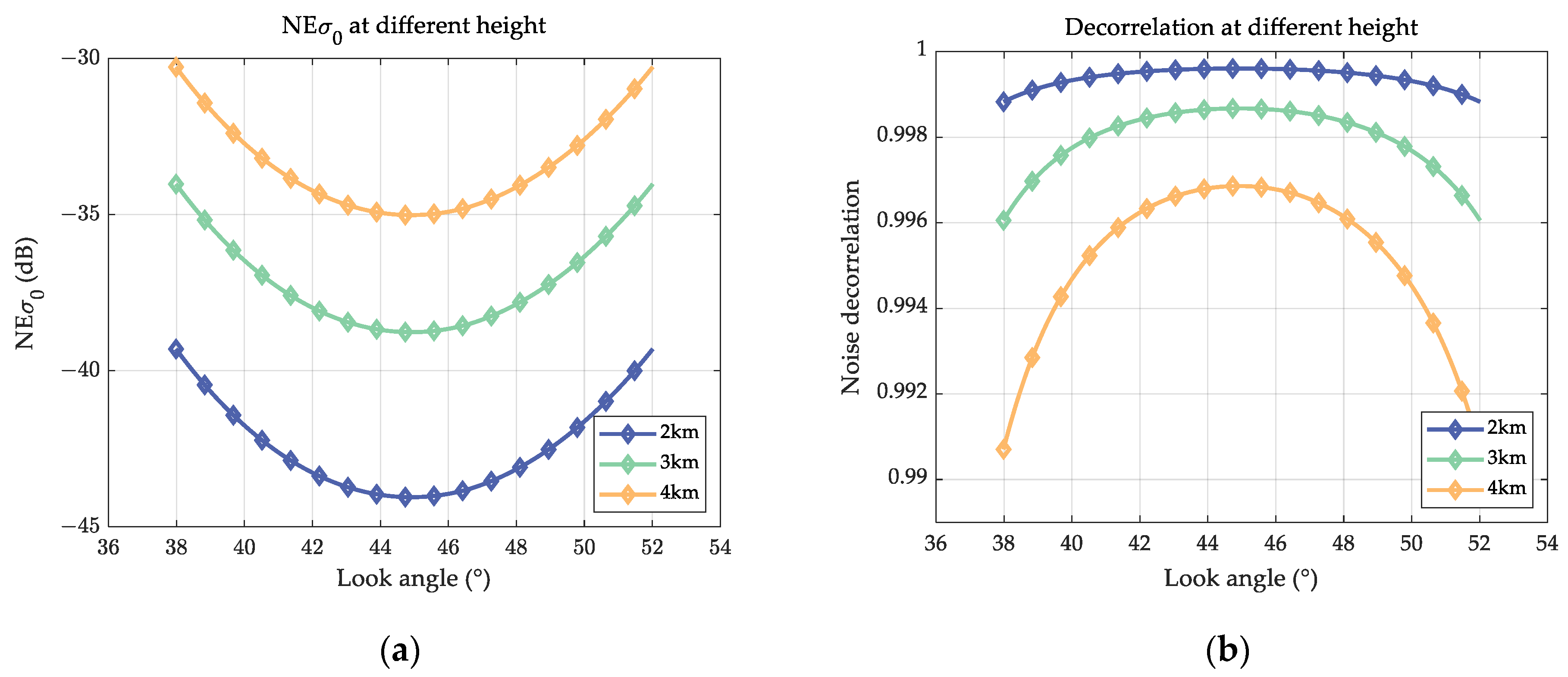
where and are the Signal-to-noise Ratio (SNR) for channels 1 and 2, respectively. The SNR can be estimated from the ratio of the echo signal to the system sensitivity ().
Figure 8a shows the curve of system sensitivity as a function of look angle at different flight altitudes. Since the system was designed with a limit of 6 km for the flight altitude design, the system sensitivity at lower altitude will be better, with higher thermal noise decorrelation, and will be optimized at the center of the scene (45°) for the same operating parameters.
2.3.2. Motion Error Analysis
Since the airborne system operates mainly in the troposphere, its position and attitude are subject to deviation from the expected trajectory due to atmospheric influences, which are more pronounced in dual-antenna systems. Firstly, motion errors may lead to inconsistencies in the doppler center frequencies of interferometric images, which directly affects the coherence of the interferograms (see Equation (7)). In addition, the motion inconsistency of the antennas introduces more errors. The residual error inconsistency component of the dual antennas can be expressed by Equation (9) [35]:
where , , and are the look angles of antennas 1 and 2 to the same illuminated target, respectively. and are the motion error of the carrier in the doppler plane in the vertical flight direction ( and directions). is carrier flight time. and is the position of antenna 1 in the zero doppler plane, is the location of the ground target point . and are the inconsistent motion errors of the two antennas in the and directions, respectively.
Considering the design of the short baseline of the ASMIS, the variation due to the difference in look angle is on the order of 10−5 at an interference height of 2000 m. Therefore, it is considered that the look angles of the two antennas are approximately equal, that is, . By designing the antenna coplanar, the error caused by the movement of the two antennas in the same direction can be reduced significantly. This is achieved by eliminating the first four terms in Equation (9).
As a result, the impact of residual error inconsistency is greatly minimized. When taking aerial photographs during a flight, we can use the same motion compensation algorithm without considering the inconsistency factor in echo imaging as long as it falls within the maximum allowed deviation value. We mainly use motion compensation based on a high-precision Inertial Measurement Unit (IMU). ASMIS has a precise navigation unit, the Applanix POS-AV610, with a Global Navigation Satellite System (GNSS) and an IMU. This navigation unit and proper postflight processing techniques ensure precise flight parameter measurability (Table 3) [39].
Before applying motion compensation, it is essential to accurately measure the coordinates of the GPS antenna, IMU, and SAR antennas. This is because the phase centers of these three components are positioned differently on the carrier. By measuring their coordinate relationship accurately, we can calculate the attitude and speed measured by the IMU to the phase center of the antenna with precise accuracy. In the actual measurement, the IMU and GPS are inside the cabin and the antenna is outside the cabin, so it is difficult to measure the relationship after installation. To ensure accurate measurements, the antenna and transition frame in the cabin can be fixed indoors. The total station can then be used to measure the relative position of each part with an accuracy of up to 0.0001 m. When calculating the phase center position of the antenna, the FRD (front, right, down) coordinate system is first established with the IMU as the origin, and the GPS position information is calibrated to the IMU, which can be obtained by Equation (10):
where and are the rotation matrix and the translation vector from GPS to IMU, respectively. These can be obtained from Equation (11):
where , , and are the angle of rotation around x, y, and z, respectively., , and are the position coordinate difference from GPS to IMU. Then, according to the position relationship between the antenna and the IMU, the IMU information is calibrated to the phase center of the antennas. This step can be obtained by Equation (12):
where , , , and are the rotation matrixes and the shift vectors from the IMU to the phase center of the antennas, respectively. Therefore, the attitude and position information of the antenna can be calculated by Equations (10)–(12).
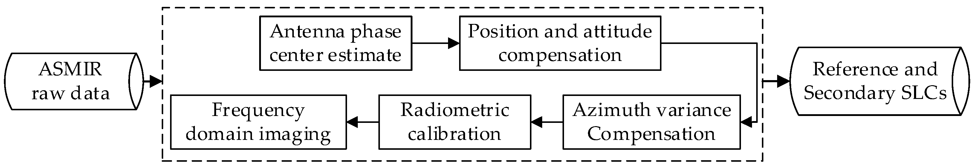
For obtaining well-focused and accurate interferometric images, we first need to perform joint motion compensation using corrected position and attitude information. After that, we can use frequency domain imaging to obtain high-quality images. Due to the large azimuth aperture of millimeter wave InSAR and the moderate swath of the airborne systems, it is more accurate and robust to choose the frequency domain for imaging after motion compensation. We performed radiometric calibration operations on the complex images after motion compensation using radiometric calibration data in the experiment area. This step is crucial in the process of transforming remote sensing data to SAR images as it helps to ensure reliability and standardization. Accurate interpretation and quantitative analysis of the images rely heavily on this process. The processing flow from the original data to the complex images is completed, as summarized in Figure 9.
2.3.3. Coherence Analysis
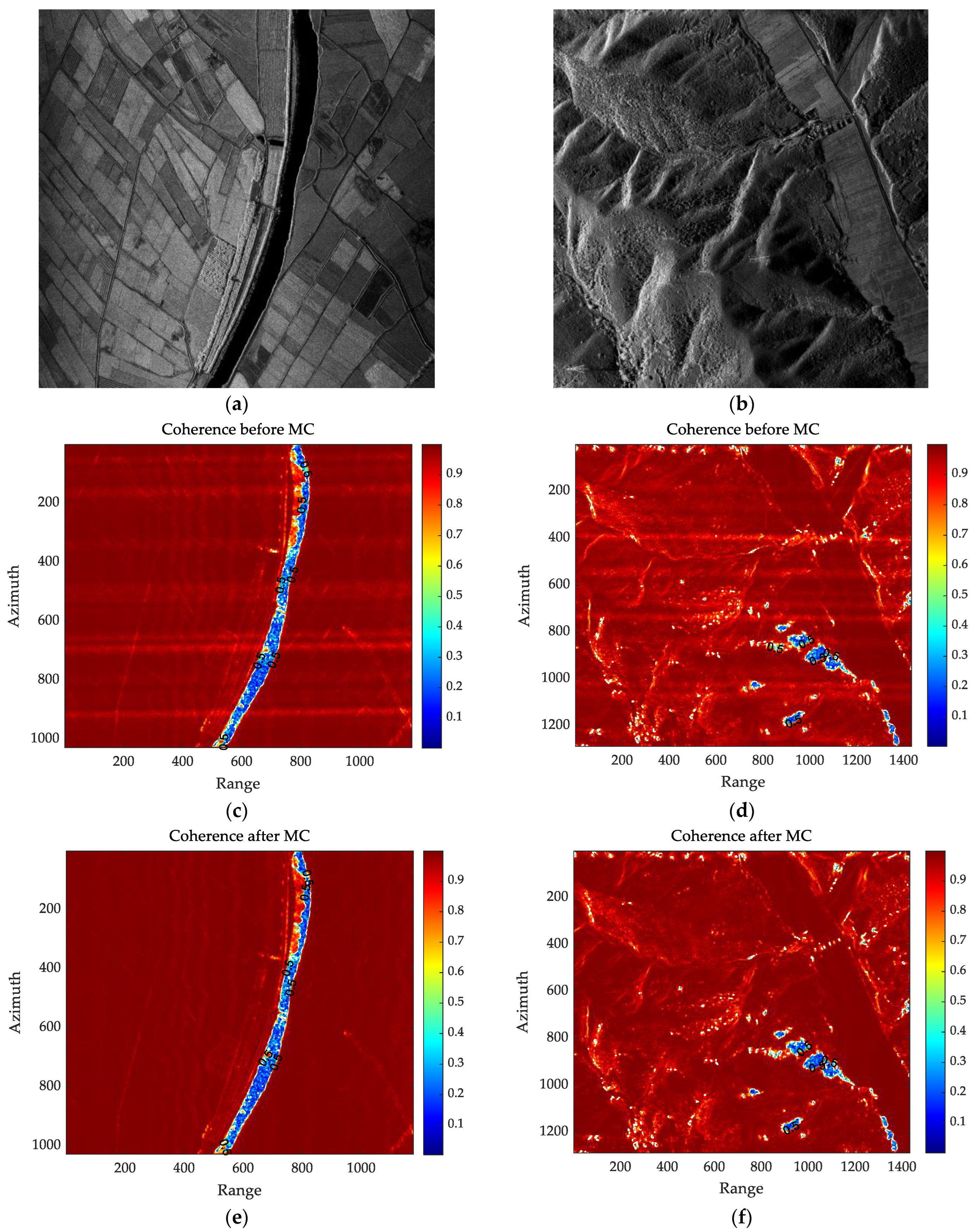
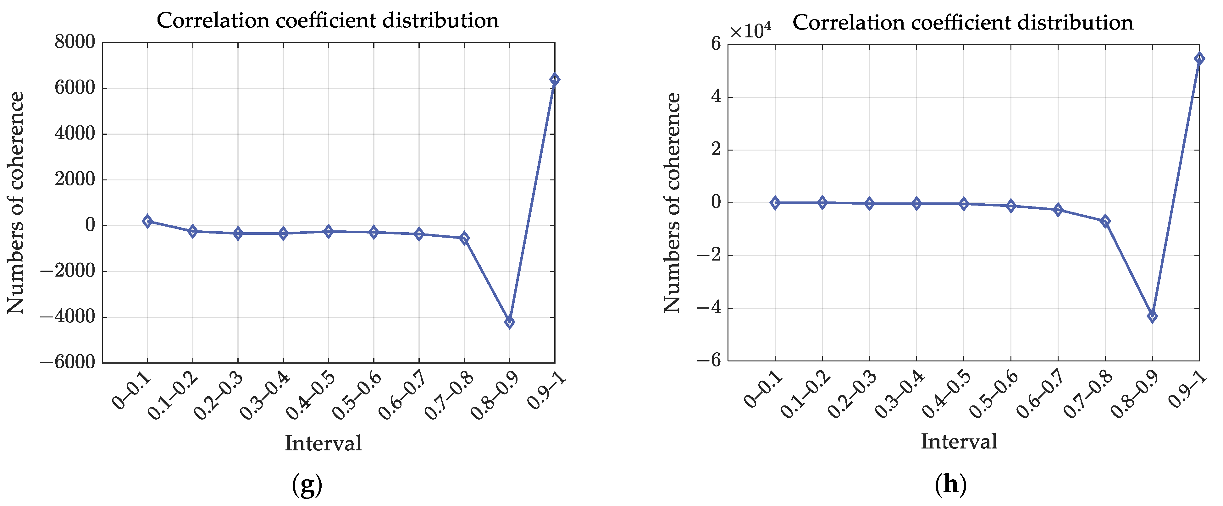
For the purpose of validating the antenna motion compensation effectiveness, we selected partial data acquired under unstable conditions from both flatland and mountainous experimental areas. Following the processing flow in Figure 9, we obtained coherence comparison results before and after dual-antennas consistent motion compensation in different regions. Figure 10a,b depict the SAR imaging results after antenna motion compensation for flatland and mountain data, respectively. Figure 10c,d show the coherence before compensation, revealing noticeable azimuthal stripes caused by motion errors. After compensation, these stripes have been eliminated in Figure 10e,f. Additionally, the differential distribution of coherence coefficients after compensation is illustrated in Figure 10g,h, indicating a reduction in areas with coherence coefficients below 0.9 and an increase in areas above 0.9.
To quantitatively describe the effect after compensation, we define a coherence optimization coefficient (), which can represent the coherence improvement of the coherence after motion compensation. The calculation is shown in Equation (13):
where is the number of incremented values within (0.9–1) in the coherence plot after motion compensation. is the total number of points in the experimental sample data. Based on this calculation, the coherence optimization coefficient of the plain experiment area and the mountain experiment area were 0.0297 (Chengde) and 0.0053 (Bayannur), respectively.
By comparing the coefficients, it can be seen that the coherence of the experimental images in the plain is better than that in the mountainous area, which is in line with the practical theory. In addition, through the consistent motion compensation of the two antennas, the coherence of the interferogram can be improved to different degrees in different experimental areas, which is sufficient to prove the stability of the ASMIS.
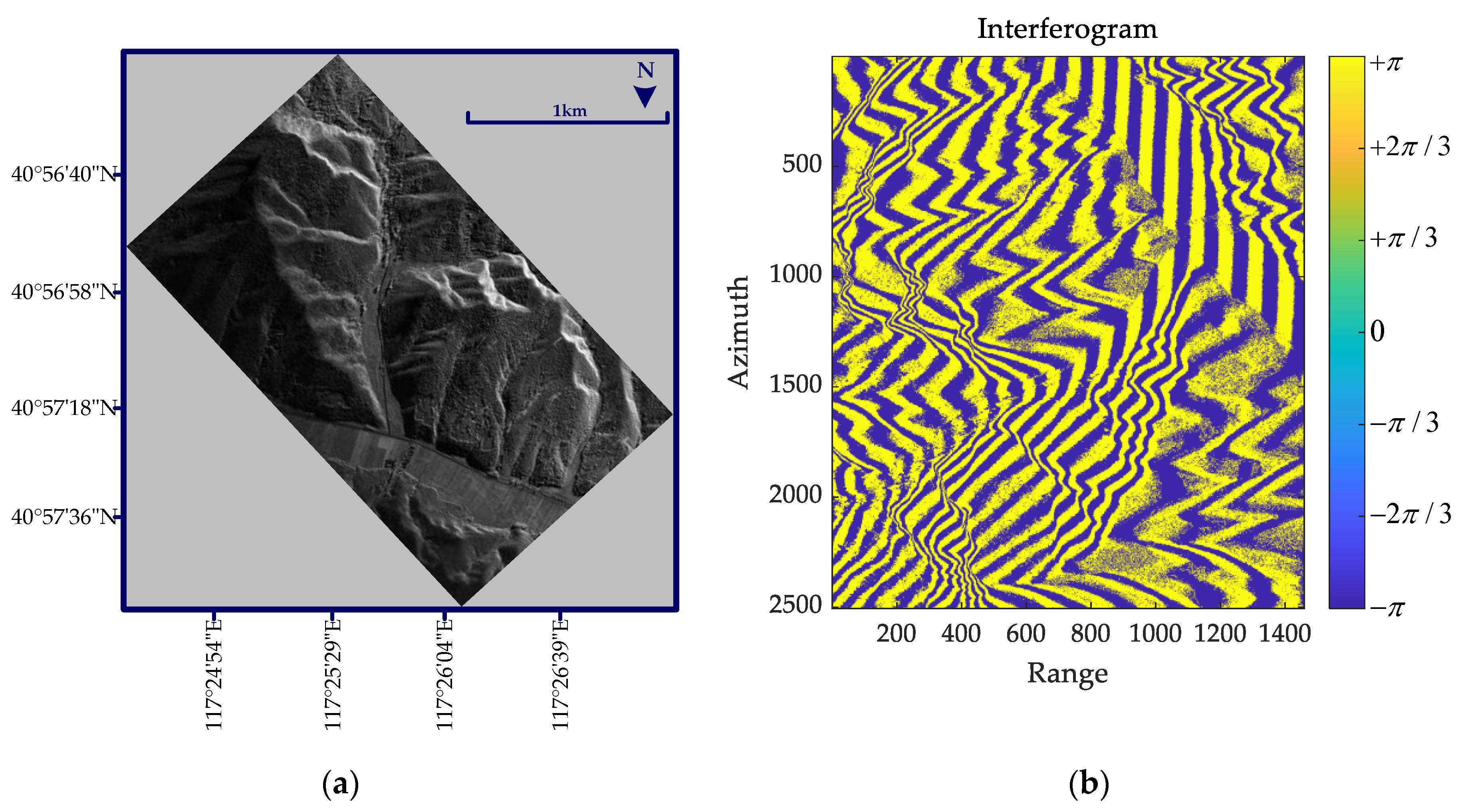
Based on the above analysis, the coherence coefficients of the ASMIS flight experiment area of about 1.4 km × 2.5 km (distance × azimuth) (Figure 11a) are statistically analyzed. After coarse registration based on the coherence function method and fine registration of cross-correlating matching parameters, the interference fringe diagram in Figure 11b is obtained after image reacquisition.
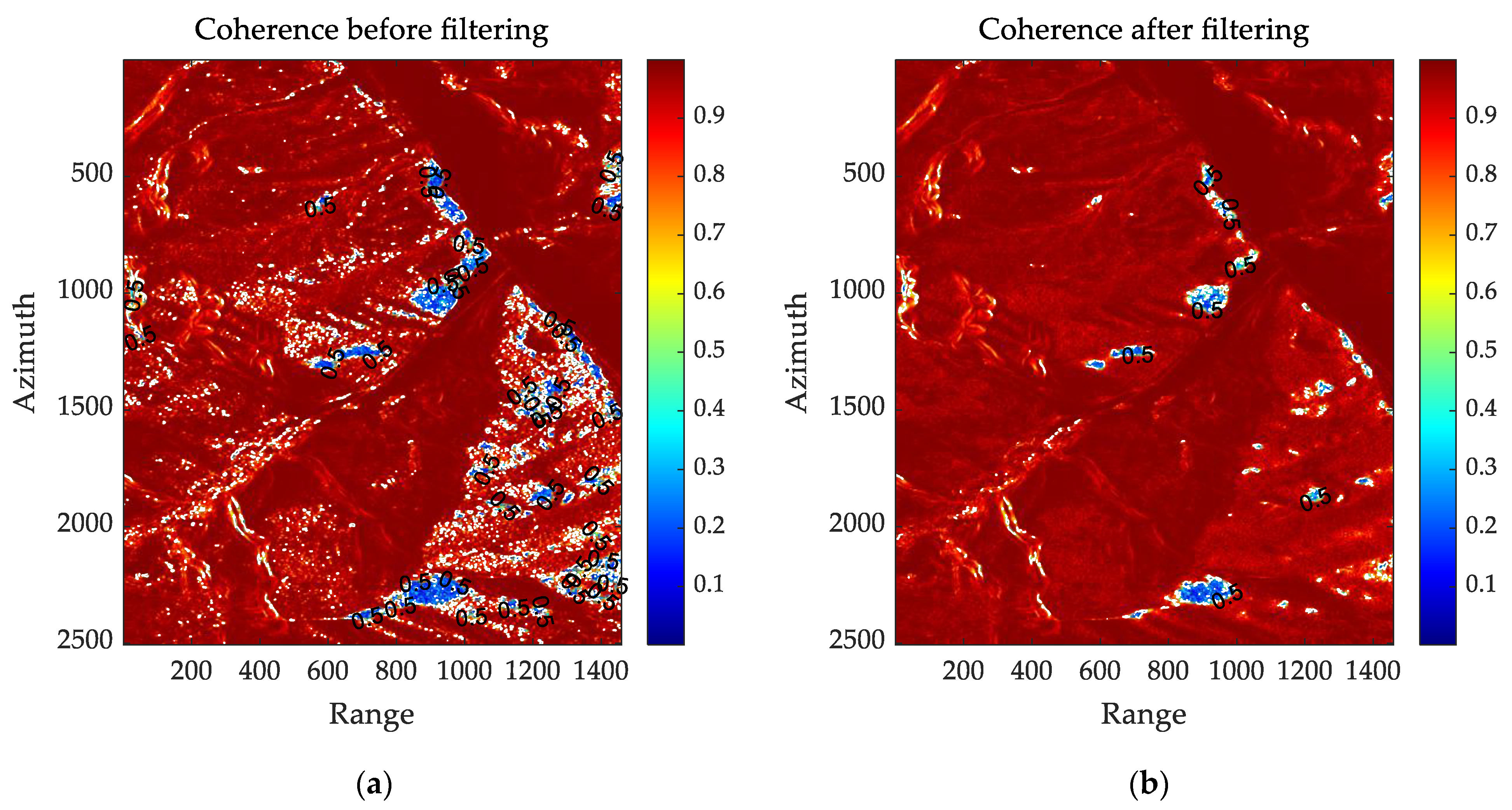
In Figure 11b, there is still a large amount of phase noise in the image after fine registration, which affects the clarity of the interferometric fringes and the subsequent phase unwrapping accuracy. It is an important operation to filter the coherence. Before generating the coherence, we use Assumed Density filtering (ADF) adaptive filtering, which can effectively remove the phase noise in the registration image and improve the phase unwrapping accuracy.
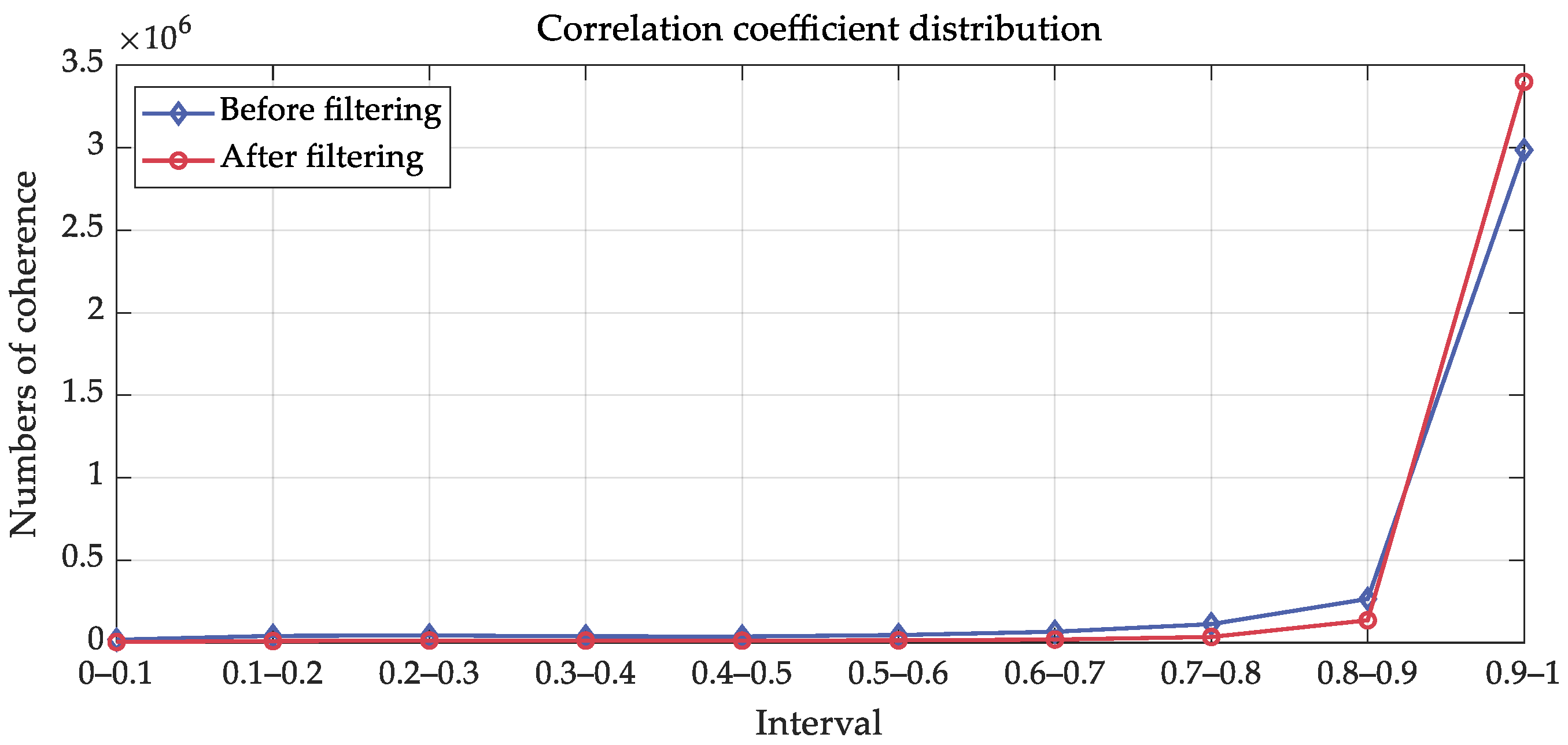
Figure 12 shows the comparison before and after filtering of the coherence. The low coherence area in the figure corresponds to the shadow area not illuminated by the InSAR. We have marked points with a coherence coefficient of 0.5 in black in the figure. By comparing the images before and after filtering, it can be seen that the region with the coherence coefficient of 0.5 after filtering is significantly reduced and the overall coherence is improved. Figure 13 shows the distribution curve of correlation coefficients; the x-axis is the segmented interval of coherence coefficients, and the y-axis is the number of coherence coefficients in each interval. It can be seen that high coherence values are mainly distributed in the interval [0.9,1.0], and are mainly concentrated above 0.95, accounting for 81% of the total.
3. System Description
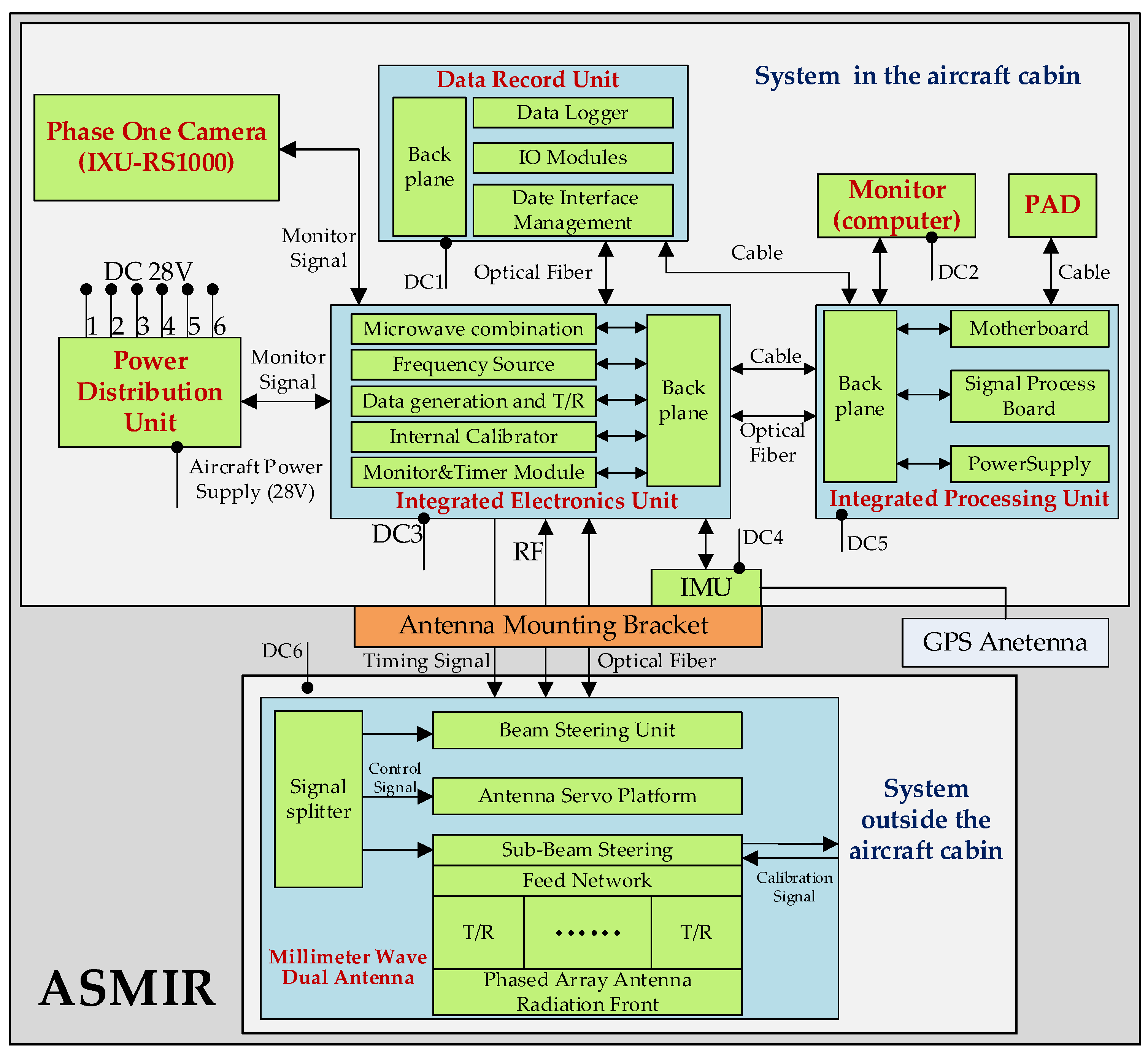
ASMIS consists of two parts: airborne equipment and ground processing system. The airborne equipment includes a Ka-band millimeter-wave SAR consisting of an antenna unit, an integrated electronics unit, an integrated processing unit, a data logging unit, a power distribution unit, a combined GPS/IMU navigation device, and a radome. The antenna unit is installed under the belly of the carrier, and the other equipment is installed on the integrated electronic equipment cabinet in the cabin. The specific structure and connection of the airborne equipment are shown in Figure 14.
The airborne equipment can generate and transmit the radar signal and obtain the original echo. The integrated electronic unit can generate the reference signal, the clock signal, the transmit signal, and the timing signal to coordinate the work of the radar system. The integrated processing unit completes the task management and real-time imaging processing of the system. The data record unit mainly realizes real-time data recording of the original echo data. The power distribution unit distributes power from the carrier to each system unit. ASMIS also integrates a Phase camera (IXU-RS1000), which can be controlled through the radar operator interface. It has an unattended mode in conjunction with the radar system. The system structure is described in more detail below.
- Antennas
ASMIS adopts 35 GHz electromagnetic waves as the signal carrier frequency, which can propagate through the atmosphere in the presence of clouds and precipitation without being greatly affected [40]. At the same time, the short-wave interferometry is weakly penetrating the ground vegetation, which makes it easy to extract the surface features of the observation area under high operations and generate DSM [41]. Polarization is a target feature in microwave remote sensing that improves identification accuracy. In practical applications, grass and roads with low scattering rates are better with horizontal polarization. Spaceborne systems for mapping also use horizontal polarization because HH polarization provides higher coherence and lower phase noise, which improves the accuracy and reliability of elevation estimation [42,43]. Therefore, the selection of HH polarization can better describe and discriminate multiple features and facilitate DSM generation.
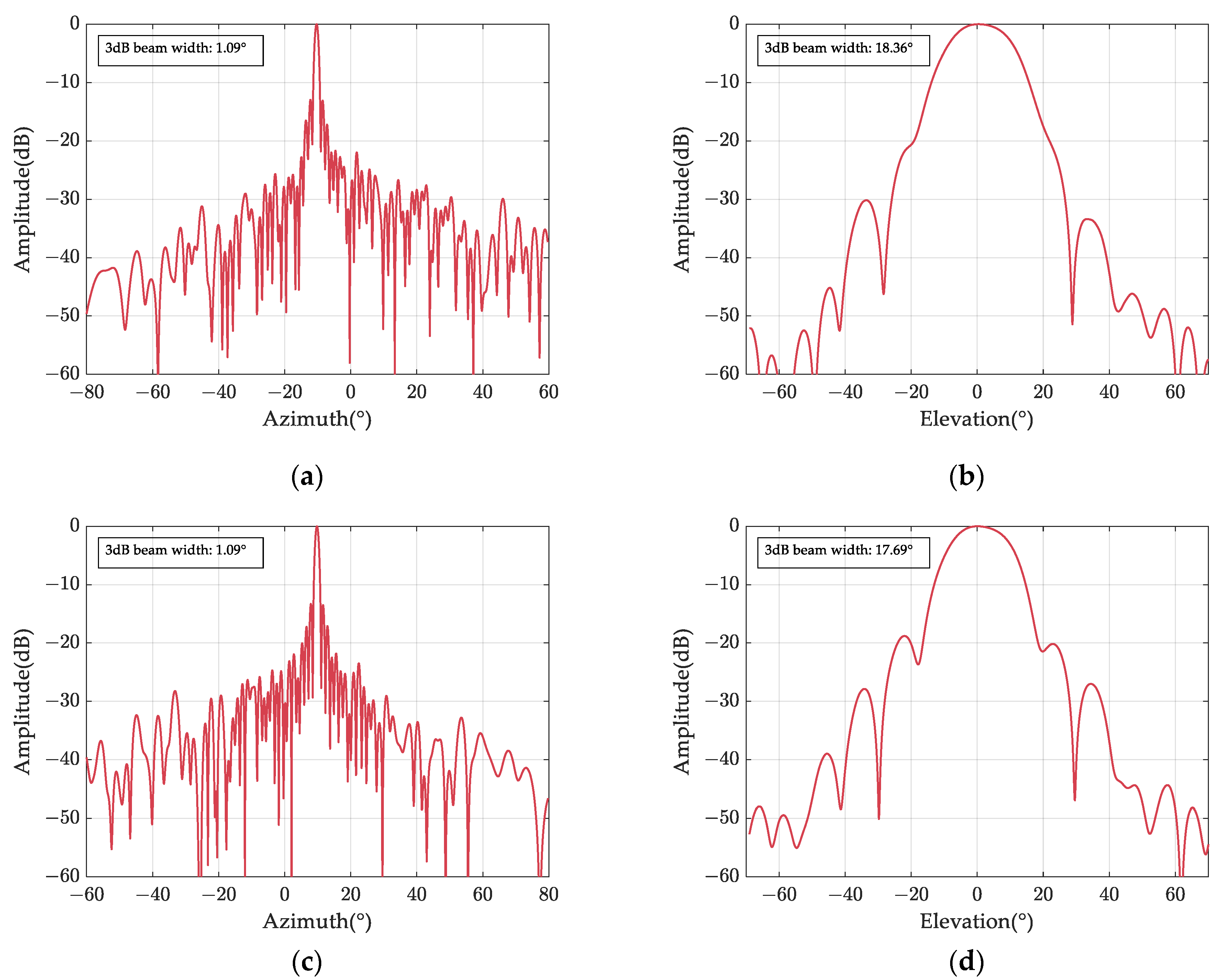
Millimeter-wave antenna using a waveguide slot array, the rectangular grid arrangement is adopted in azimuth, and the design of the choke slot increases the isolation. To achieve the scanning requirements, the group array unit is spaced in 6 mm intervals. The individual antenna specifications were as follows: 64 units in azimuth and 1 unit in range, with the array layer of the electrical dimensions of 384 mm (azimuth) × 27 mm (range). Each unit is driven by a single channel T/R module, and four gaps in each waveguide radiate electromagnetic waves. In the case of uniform distribution, the antenna directivity coefficient is 32.5 dB, and the difference between high- and low-frequency directivity coefficients is 1 dB [44]. In the normal direction, the maximum side lobe of the two main plane directions of the antenna array azimuth and distance is lower than −12dB, and the side lobe outside the main plane is not more than this value. The planar near-field test was used for the antenna radiation diagram, and the test results are shown in Figure 15 [45].
- 2.
- Integrated Electronic Unit
The unit can be used to realize the generation, processing, and transmission of radar signals, as well as the control and monitoring of the radar. It consists of the following parts: a reference frequency source is used to generate initial radar signals, including reference signals, clock signals, timing signals, and control signals, and to monitor the output of each signal. The microwave combination and internal calibrator are used to complete the amplified output of Radio frequency (RF) signals and the duplex transmission of echo signals. As well as the formation of reference calibration, these also receive calibration and transmit calibration signals.
The transmitter and receiver (T/R) channel is based on Low-Temperature Co-fired Ceramic (LTCC) technology, which is used for secondary frequency conversion, filtering and amplifying the initial signal to be output to the microwave combining module. It is also used for down-conversion, Manual Gain Control (MGC) adjustment, signal amplification, and quadrature demodulation of the low-noise amplified echo signal.
The data generation unit is used to extract, filter, and quantize the echo signal, pack it with auxiliary data into frames, and format them to obtain the echo data. The monitor and timer module are used to set parameters, generate signals, and monitor the system. It can also calculate the wave control code according to the working mode and parameters of the radar and the attitude data of the carrier. This is then sent to the antenna unit to realize the real-time motion compensation and beam control of the radar, as well as the servo control of the antennas.
- 3.
- Integrated Processing Unit
The integrated processing unit is composed of the main board, signal processing board, power supply board, and backplane. It manages radar missions, displays imaging, controls recording operations, and summarizes monitoring data through man-machine interaction. Additionally, it has an unmanned mode of operation that allows it to read the IMU’s raw data and forward it to the data recording unit. In the system, the backplane is used to interconnect high-speed signals and power signals between boards within the unit.
4. Experiment and Interferometric Processing
4.1. Flight Experiment Areas
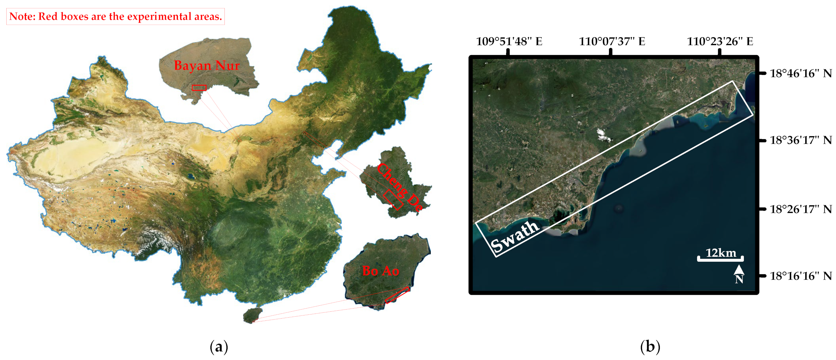
ASMIS carried out several flight experiments in Boao, Bayannur, and Chengde aboard the Cessna 208B, with the experimental areas covering a wide range of landforms (Figure 16a). The details are as follows: in the Boao experimental area, considering the experimental purpose of large swath observation, a long route (Figure 16b) was designed with a flight altitude of 4000 m. The average elevation of the irradiated area was 50 m, and the terrain was dominated by the coastal area (including the coastline). The latitude and longitude range of the covered area is 18.315°N~18.753°N, 109.783°E~110.473°E.
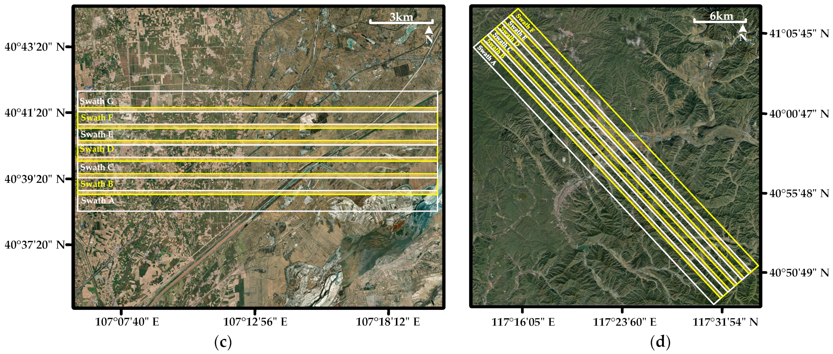
In the Bayannur experimental area, the flight altitude was 3000 m and the average elevation of the irradiated area was 1003m, which contained typical landscapes such as plains and farmland. A total of seven strips were designed in the Bayannur experimental area (Figure 16c), with a 20% overlap between neighboring strips (see the yellow transparent area of neighboring strips in Figure 16c). The latitude and longitude range of the coverage area is 40.638°N~40.691°N, 107.098°E~107.335°E. In addition, we set up a radiometric calibration field in the flight coverage area for subsequent radiometric calibration processing. The calibration experiment field site was selected and set at a large area with flat terrain and weak ground object backscattering. Radiometric calibration eliminates the influence of sensor characteristics, terrain, and other factors on the SAR image radiation value and makes the image reflect the real radiation characteristics of ground objects [46].
In the Chengde experimental area, the flight altitude was 2800 m, and the average altitude of the irradiated area was 460 m. Due to the undulating topography and the predominance of mountainous and forested areas, the Chengde experimental area is prone to a higher proportion of layovers and shadows caused by SAR squint imaging. As a result, the interferometric phases obtained may appear unconnected or even full of noise, leading to a degradation in the accuracy of the DEM [47]. To compensate for areas of geometric aberration at one angle, a common approach is to combine multi-angle observations of the same region [48].
Therefore, we designed an antiparallel flight experiment in the Chengde experimental area, and the system worked with a left-side view for all six strips (Figure 16d). When the carrier completes a route on a particular strip, it follows an “8” turnaround flight pattern and flies in the opposite direction. This helps to reduce the errors caused by the POS system when collecting data from the same irradiated area multiple times. There is a 20% overlap between neighboring strips (see the yellow transparent area of the neighboring strips in Figure 16d), and the latitude and longitude range of the covered area is 40.813°N~41.119°N, 117.204°E~117.578°E. In addition, a few GCPs were set up in an area of 2.3 km × 2.6 km in size at the Chengde Flight Center (see Section 5.1) to provide a basis for subsequent accuracy assessment.
During aerial operations, the POS recorded its 3D coordinates, attitude angle, velocity, acceleration, and other information at a frequency of 500 Hz. The flight parameters of each experimental area are shown in Table 4.
4.2. Interferometric Processing
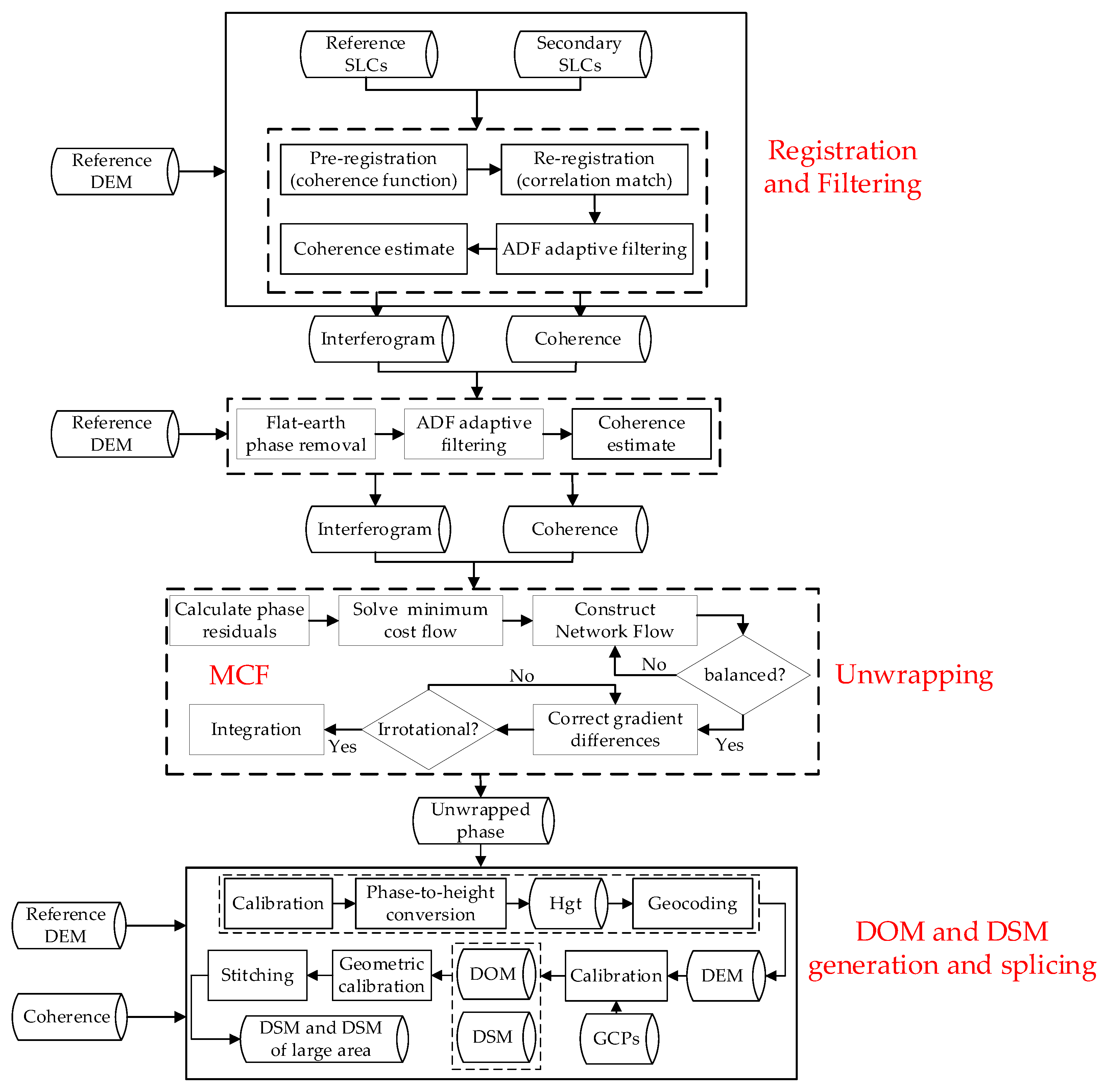
Once motion compensation and imaging are completed, the acquired complex image requires several additional processing steps to generate the final coherence image. These steps include registration, filtering, decorrelation, and coherence estimation. After that, the DEM is obtained by performing unwrapping, calibration, phase-to-height conversion, and geocoding. Finally, the large-scale DSM and DOM images are generated by performing GCPs calibration, geometry calibration, and image stitching. The precise alignment and filtering of the images have been explained in detail in the decorrelation analysis, which is covered in Section 2. The specific steps involved in this process are illustrated in Figure 17. However, we will not go into further detail on this aspect here as our focus is on the other primary processing flows.
- Unwrapping
Phase unwrapping is the process of reducing the phase values wrapped in to their true continuous phase values. MCF (Minimum Cost Flow) is a phase unwrapping algorithm. The advantage of the MCF algorithm is that it is extremely robust and accurate and can deal with complex nonlinear problems. The steps of the MCF algorithm to realize unwrapping are shown in Figure 17. We remove the image of the flat earth phase first, and perform secondary ADF filtering on the interferograms and coherence before unwrapping. During unwrapping, we choose not to process the image in chunks, but to treat the whole image as a network flow map, which can avoid the error propagation at the boundary of chunks and improve the accuracy of unwrapping.
- 2.
- Generation and Splicing of DOM and DSM
The interferometric phase of InSAR after phase unwrapping is calibrated and converted to altitude (HGT) by using the interferometric baseline and the slant range. Then, the HGT is geocoded to obtain the DEMs by using the orbit parameters and the range–Doppler equation. The orthorectification and the control point elevation calibration are performed to obtain the DOMs and the DSMs by using the DEM and the SAR intensity image. Finally, the geometric calibration and the mosaic are applied to the DOM and the DSM to obtain the large-area DSM and DOM images. The specific process is shown in Figure 17.
5. Results
5.1. Result of Evaluation Accuracy
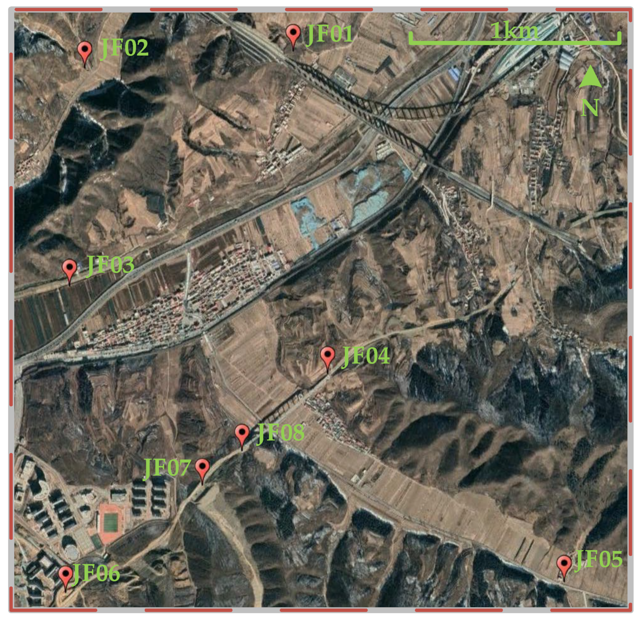
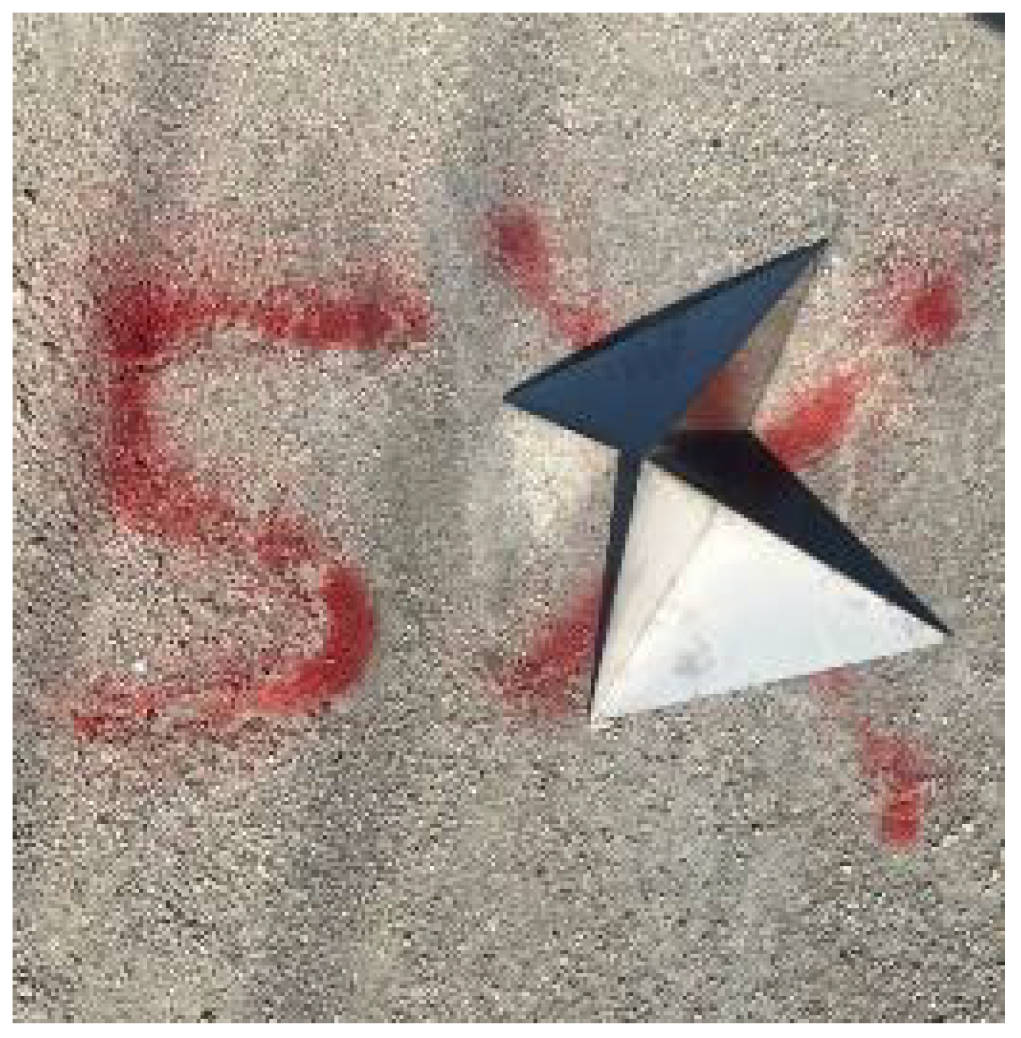
In the Chengde experimental area, we used a dispersed arrangement of eight calibrators as GCPs, including control point mapping the area in Figure 18, covering the area in the latitude and longitude range of 40.958°N~40.979°N to 117.375°E~117.406°E. When positioning the GCPs, we opted for areas with level terrain, limited vegetation, consistent characteristics, and strong echo intensity, based on the recommendations for distributed placement. Since the flight path was two-way, the calibration points were arranged in pairs, facing in opposite directions. Figure 19 depicts the location of calibration point No.5, which is part of such a pair, and its placement ensures the reliability of data processing in both directions.
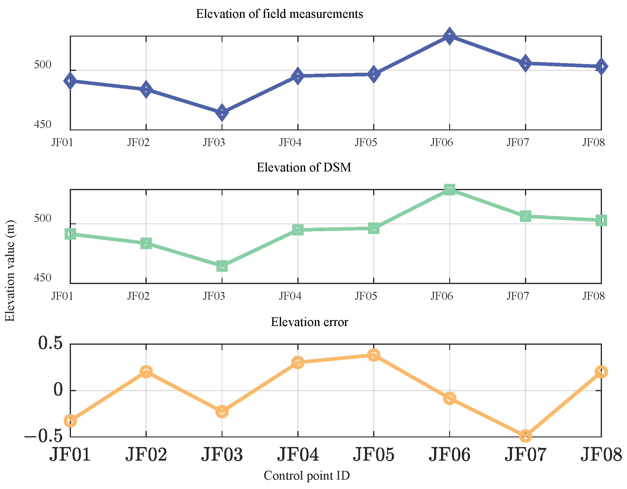
The evaluation of interferometric elevation measurement accuracy is realized by testing the DSM products. The elevation accuracy of DSM data products is mainly examined by using the GCPs of the field measurements. The elevation measurement accuracy is characterized by using the elevation RMSE of the GCPs, and the calculation is obtained in Equation (14):
where is the number of GCPs, is the elevation of the DSM, is the measured elevation of the GCPs, and is the elevation RMSE. The statistical results of the GCPs are shown in Figure 20 and Table 5, which show that the elevation RMSE is 0.30 m. In addition, by analyzing the field checkpoints arranged in the modified area, the elevation RMSE of checkpoints is less than 0.82 m in altitude and 3 m horizontally. According to the requirements of the Chinese surveying and mapping industry, ASMIS can satisfy the production standards of 1:5000 [49].
5.2. Results of DOM and DSM
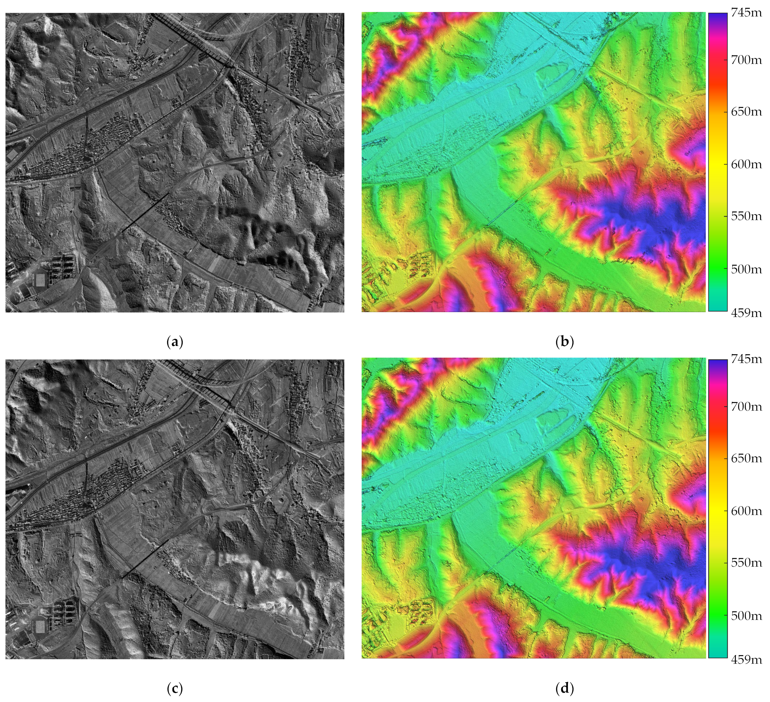
Through geometric calibration, image stitching, and grid interpolation of DSM obtained after processing the regional data of the Chengde center experimental area, a standard map sheet with a resolution of 0.3 m and a mapping scale of 1:5000 was obtained, as shown in Figure 21. Figure 21a,b show the DOM and DSM results obtained by the carrier flying from east to west, and Figure 21c,d show the DOM and DSM results obtained by the carrier flying from west to east, respectively. To overcome the challenge of shadowing caused by undulating terrain, a useful technique is to combine data from antiparallel flights. This integration results in a multi-look image of the same observation area, which is highly beneficial for mapping applications. This approach may effectively resolve the problem of undulating terrain, making it important for all-terrain mapping and applications.
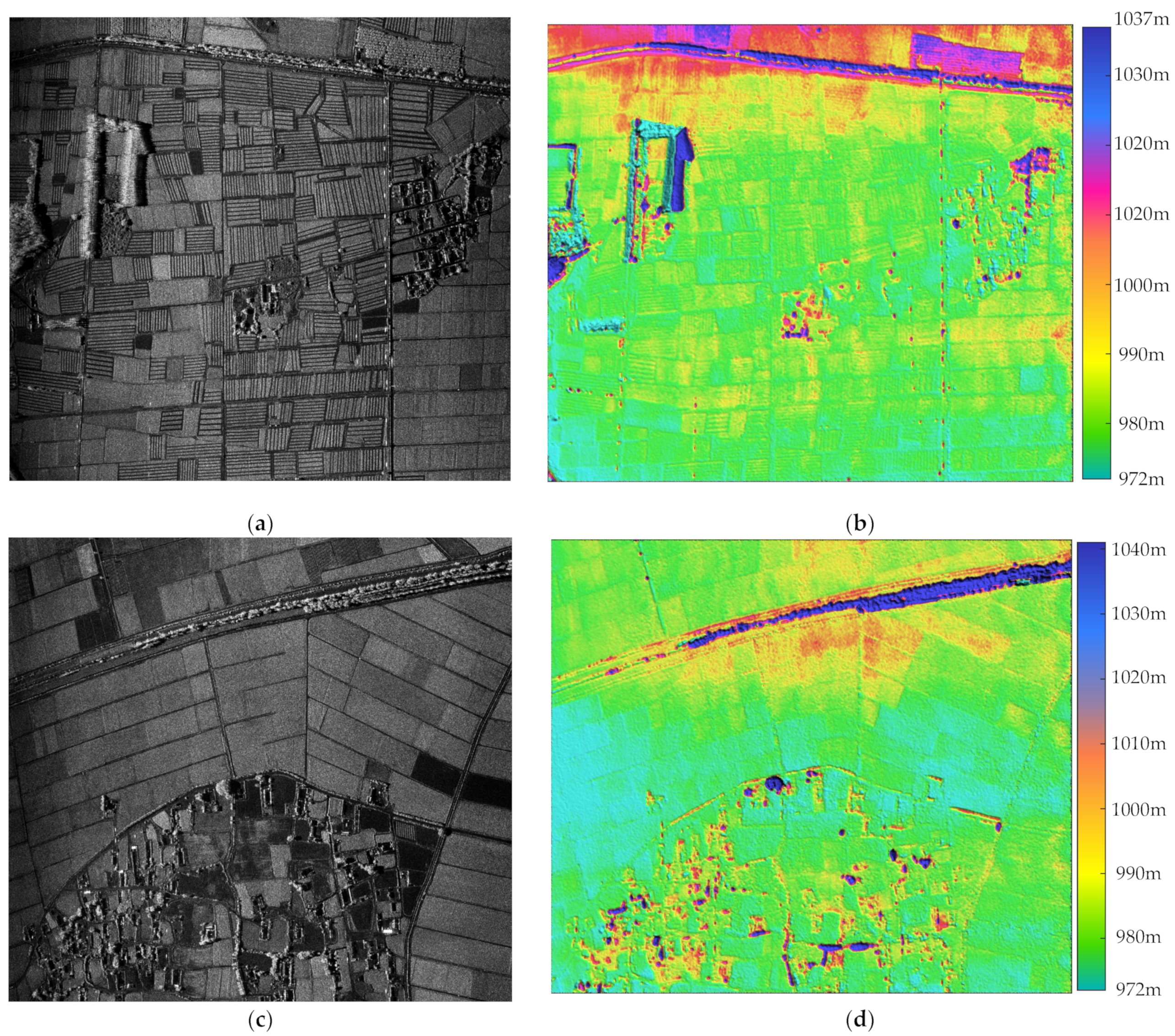
In the Bayannur experimental area, the terrain is dominated by plains and deserts, and no two-way flight experiment was designed considering its flat terrain with less superimposed layover and shadow. The findings of the flat region acquired after processing are illustrated in Figure 22. When we integrate high-resolution SAR imaging images with the DSM results of the experimental area, we can enhance the accuracy of feature recognition and classification. This is of significant importance in terrain analysis.
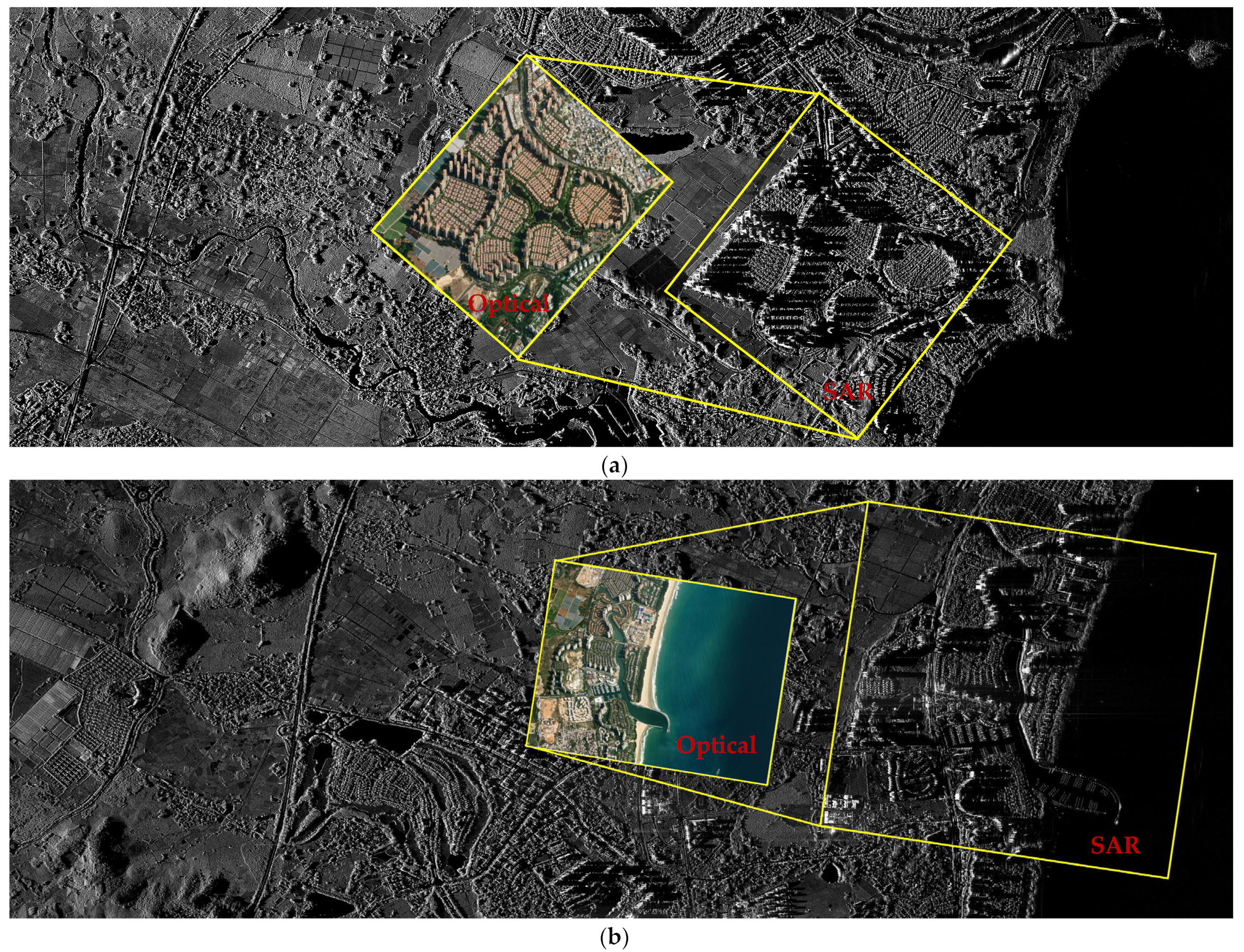
In the Boao experimental area, the primary objective was to test the large swath imaging capability of ASMIS. To achieve this, a center look angle of 70° was set up, and the imaging results with 0.3 m resolution were obtained after transportation and imaging processing. Figure 23a,b show the results of this high-resolution, wide-area observation. This can significantly improve mapping efficiency and information along the coastline. By utilizing optical images, it becomes possible to accurately differentiate between land and water in coastal areas. This method can lead to numerous opportunities for further research and practical applications in this field.
6. Conclusions and Discussion
In this paper, we present a millimeter-wave InSAR system (ASMIS). The sensitivity effects are analyzed in detail based on the system design. ASMIS carried out topographic modeling experiments in the plains, mountains, and coastal areas of China, and the data were processed and analyzed. The experimental results prove the theoretical analysis, as well as the performance and stability of the system. The most important conclusions of this paper are as follows:
- Short-baseline airborne InSAR is capable of combining elevation accuracy and coherence. ASMIS has obtained the correlation coefficient of better than 0.95 within 81% of the area in mountainous areas. By designing a few GCPs in the Chengde experimental area, ASMIS realizes the requirement of 1:5000 topographic mapping. The coordinate RMSE of the checkpoints within the obtained DSM is less than 0.82 m in altitude and 3 m horizontally. The RMSE of the GCPs within the obtained DSM is less than 0.3 m in altitude.
- The motion inconsistency error of short-baseline InSAR can be ignored to some extent. The processing directly compensates for the motion consistency of the reference and secondary antennas, which can simplify the algorithm to improve efficiency.
- The multiple work modes of ASMIS have obtained great experimental results, including 0.1 m × 0.1 m (azimuth × range) resolution imaging, and 0.3 m × 0.3 m (azimuth × range) resolution wide-swath imaging.
- Undulating terrains can cause shadow, but the antiparallel flight experiments can provide an effective solution to this problem.
The system proposed in this paper is advanced in performance and stability. Compared with the Ka-Band Fixed-Baseline InSAR developed by the Beijing Institute of Radio Measurement and the AXIS (Airborne X-band Interferometric SAR) system developed by the Institute for Remote Sensing of Environment (IREA), National Research Council (CNR) [39,50], ASMIS has a better spatial resolution (0.1 m), fewer GCPs required for elevation assessment, and more imaging modes. We take into account the effects of the undulating terrain, and design antiparallel flight experiments in mountainous areas to obtain data. The work in this paper focuses on system design and sensitivity analysis. The data were processed, calibrated across strips, and spliced to obtain a 1:5000 DSM product. The results demonstrate the accuracy of the system on topographic mapping. However, the system still has the following limitations to be developed for further research:
- In the elevation accuracy, a laser baseline measurement system can be considered to compensate for the deformation of the facilities. This can control the baseline length and angle errors to 0.1 mm and 0.002°, respectively, and further improve the elevation error according to the theoretical analysis.
- The experimental area data is multi-temporal, multi-angle, and multi-parameter. It can support more remote sensing applications such as feature classification and deformation assessment.
- At present, only the antiparallel flight data of the Chengde experimental area has been processed independently. Joint correction and splicing processing are needed in the future.
Author Contributions
Conceptualization, L.W. and Y.L.; methodology, L.W. and Y.L; software, L.W.; validation, L.W., Y.L. and Q.C.; formal analysis, L.W. and X.Z.; investigation, S.Z.; resources, S.C.; data curation, Y.L.; writing—original draft preparation, L.W. and Y.L.; writing—review and editing, L.W.; visualization, L.W.; supervision, Q.C.; project administration, Y.L. All authors have read and agreed to the published version of the manuscript.
Funding
This research received no external funding.
Data Availability Statement
Data available on request due to privacy.
Acknowledgments
The authors would like to thank the reviewers and the editor for their careful and professional comments.
Conflicts of Interest
The authors declare no conflicts of interest.
References
- Rosen, P.A.; Hensley, S.; Joughin, I.R.; Li, F.K.; Madsen, S.N.; Rodriguez, E.; Goldstein, R.M. Synthetic aperture radar interferometry. Proc. IEEE 2000, 88, 333–382. [Google Scholar] [CrossRef]
- Schulz-Stellenfleth, J.; Lehner, S. Ocean wave imaging using an airborne single pass across-track interferometric SAR. IEEE Trans. Geosci. Remote Sens. 2001, 39, 38–45. [Google Scholar] [CrossRef]
- Rocca, F.; Prati, C.; Guarnieri, A.M.; Ferretti, A. Sar Interferometry And Its Applications. Surv. Geophys. 2000, 21, 159–176. [Google Scholar] [CrossRef]
- Hagberg, J.O.; Ulander, L.M.H. Repeat-pass SAR interferometry over forested terrain. IEEE Trans. Geosci. Remote Sens. 1995, 33, 331–340. [Google Scholar] [CrossRef]
- Hornacek, M.; Wagner, W.; Sabel, D.; Truong, H.L.; Snoeij, P.; Hahmann, T.; Diedrich, E.; Doubkova, M. Potential for High Resolution Systematic Global Surface Soil Moisture Retrieval via Change Detection Using Sentinel-1. IEEE J. Sel. Top. Appl. Earth Obs. Remote Sens. 2012, 5, 1303–1311. [Google Scholar] [CrossRef]
- Snoeij, P.; Attema, E.; Davidson, M.; Duesmann, B.; Floury, N.; Levrini, G.; Rommen, B.; Rosich, B. Sentinel-1 radar mission: Status and performance. IEEE Aerosp. Electron. Syst. Mag. 2010, 25, 32–39. [Google Scholar] [CrossRef]
- Zebker, H.A.; Werner, C.L.; Rosen, P.A.; Hensley, S. Accuracy of topographic maps derived from ERS-1 interferometric radar. IEEE Trans. Geosci. Remote Sens. 1994, 32, 823–836. [Google Scholar] [CrossRef]
- Rufino, G.; Moccia, A.; Esposito, S. DEM generation by means of ERS tandem data. IEEE Trans. Geosci. Remote Sens. 1998, 36, 1905–1912. [Google Scholar] [CrossRef]
- Roth, A.; Werninghaus, R. Status of the TerraSAR-X Mission. In Proceedings of the 2006 IEEE International Symposium on Geoscience and Remote Sensing, Denver, CO, USA, 31 July–4 August 2006; pp. 1918–1920. [Google Scholar]
- Krieger, G.; Moreira, A.; Fiedler, H.; Hajnsek, I.; Werner, M.; Younis, M.; Zink, M. TanDEM-X: A Satellite Formation for High-Resolution SAR Interferometry. IEEE Trans. Geosci. Remote Sens. 2007, 45, 3317–3341. [Google Scholar] [CrossRef]
- Song, Y.; Sun, Z. Analysis and Verification of The Characteristics of The Sharp-Peaked and Heavy-Tailed of Gf-3 Sar Image. In Proceedings of the 2018 Fifth International Workshop on Earth Observation and Remote Sensing Applications (EORSA), Xi’an, China, 18–20 June 2018; pp. 1–5. [Google Scholar]
- Hua, L.; Zhenning, L.; Kaiyu, L.; Mingshan, R.; Yunkai, D. The Present Situation and Development for Spaceborne Synthetic Aperture Radar Antenna Arrays. In Antenna Arrays; Hussain, M.A.-R., Nijas, K., Sulaiman, T., Aldebaro, K., Eds.; IntechOpen: Rijeka, Croatia, 2022; p. Ch.2. [Google Scholar]
- Wang, X.-G.; Wang, Z.-Q.; Yang, X.; Liu, W. Analysis of Spaceborne Dual-antenna InSAR System Characteristic Under Flexible Baseline Oscillation. J. Electron. Inf. Technol. 2011, 33, 1114–1118. [Google Scholar] [CrossRef]
- Eriksson, L.E.B.; Santoro, M.; Fransson, J.E.S. Temporal Decorrelation for Forested Areas Observed in Spaceborne L-band SAR Interferometry. In Proceedings of the IGARSS 2008—2008 IEEE International Geoscience and Remote Sensing Symposium, Boston, MA, USA, 7–11 July 2008; pp. V-283–V-285. [Google Scholar]
- Ahmed, R.; Siqueira, P.; Hensley, S.; Chapman, B.; Bergen, K. A survey of temporal decorrelation from spaceborne L-Band repeat-pass InSAR. Remote Sens. Environ. 2011, 115, 2887–2896. [Google Scholar] [CrossRef]
- Younis, M.; Metzig, R.; Krieger, G. Performance prediction of a phase synchronization link for bistatic SAR. IEEE Geosci. Remote Sens. Lett. 2006, 3, 429–433. [Google Scholar] [CrossRef]
- Krieger, G.; Younis, M. Impact of oscillator noise in bistatic and multistatic SAR. IEEE Geosci. Remote Sens. Lett. 2006, 3, 424–428. [Google Scholar] [CrossRef]
- Rodriguez-Cassola, M.; Baumgartner, S.V.; Krieger, G.; Moreira, A. Bistatic TerraSAR-X/F-SAR Spaceborne–Airborne SAR Experiment: Description, Data Processing, and Results. IEEE Trans. Geosci. Remote Sens. 2010, 48, 781–794. [Google Scholar] [CrossRef]
- Kropatsch, W.G.; Strobl, D. The generation of SAR layover and shadow maps from digital elevation models. IEEE Trans. Geosci. Remote Sens. 1990, 28, 98–107. [Google Scholar] [CrossRef]
- Wen, N.; Zeng, F.; Dai, K.; Li, T.; Zhang, X.; Pirasteh, S.; Liu, C.; Xu, Q. Evaluating and Analyzing the Potential of the Gaofen-3 SAR Satellite for Landslide Monitoring. Remote Sens. 2022, 14, 4425. [Google Scholar] [CrossRef]
- Brenner, A.R.; Roessing, L. Radar Imaging of Urban Areas by Means of Very High-Resolution SAR and Interferometric SAR. IEEE Trans. Geosci. Remote Sens. 2008, 46, 2971–2982. [Google Scholar] [CrossRef]
- Magnard, C.; Frioud, M.; Small, D.; Brehm, T.; Essen, H.; Meier, E. Processing of MEMPHIS Ka-Band Multibaseline Interferometric SAR Data: From Raw Data to Digital Surface Models. IEEE J. Sel. Top. Appl. Earth Obs. Remote Sens. 2014, 7, 2927–2941. [Google Scholar] [CrossRef]
- Hensley, S.; Chapin, E.; Freedman, A.; Le, C.; Madsen, S.; Michel, T.; Rodriguez, E.; Siqueira, P.; Wheeler, K. First P-band results using the GeoSAR mapping system. In Proceedings of the IGARSS 2001, Scanning the Present and Resolving the Future, Proceedings, IEEE 2001 International Geo-science and Remote Sensing Symposium (Cat. No.01CH37217), Sydney, NSW, Australia, 9–13 July 2001; Volume 121, pp. 126–128. [Google Scholar]
- Satake, M.; Matsuoka, T.; Umehara, T.; Kobayashi, T.; Nadai, A.; Uemoto, J.; Kojima, S.; Uratsuka, S. Calibration experiments of advanced X-band airborne SAR system, Pi-SAR2. In Proceedings of the 2011 IEEE International Geoscience and Remote Sensing Symposium, Vancouver, BC, Canada, 24–29 July 2011; pp. 933–936. [Google Scholar]
- Sun, L.; Zhang, C.; Hu, M. Perfermance analysis and data processing of the airborne X-band insar system. In Proceedings of the 2007 1st Asian and Pacific Conference on Synthetic Aperture Radar, Huangshan, China, 5–9 November 2007; pp. 541–545. [Google Scholar]
- Li, D.-J.; Liu, B.; Pan, Z.-H.; Mao, Y.-F.; Qiao, M.; Teng, X.-M.; Li, L.-C. Airborne MMW InSAR Interferometry with Cross-Track Three-Baseline Antennas. In Proceedings of the 9th European Conference on Synthetic Aperture Radar, Nuremberg, Germany, 23–26 April 2012; pp. 301–303. [Google Scholar]
- Brozzetti, F.; Boncio, P.; Cirillo, D.; Ferrarini, F.; De Nardis, R.; Testa, A.; Liberi, F.; Lavecchia, G. High-Resolution Field Mapping and Analysis of the August–October 2016 Coseismic Surface Faulting (Central Italy Earthquakes): Slip Distribution, Parameterization, and Comparison with Global Earthquakes. Tectonics 2019, 38, 417–439. [Google Scholar] [CrossRef]
- Fernandez-Diaz, J.C.; Telling, J.; Glennie, C.; Shrestha, R.L.; Carter, W.E. Rapid change detection in a single pass of a multichannel airborne lidar. In Proceedings of the 2017 IEEE International Geoscience and Remote Sensing Symposium (IGARSS), Fort Worth, TX, USA, 23–28 July 2017; pp. 1304–1307. [Google Scholar]
- Mora, O.E.; Lenzano, M.G.; Toth, C.K.; Grejner-Brzezinska, D.A.; Fayne, J.V. Landslide Change Detection Based on Multi-Temporal Airborne LiDAR-Derived DEMs. Geosciences 2018, 8, 23. [Google Scholar] [CrossRef]
- Jin, B.; Guo, J.; Wei, P.; Su, B.; He, D. Multi-baseline InSAR phase unwrapping method based on mixed-integer optimisation model. IET Radar Sonar Navig. 2018, 12, 694–701. [Google Scholar] [CrossRef]
- Li, J.; Wang, G.; Wei, L.; Lu, Y.; Hu, Q. Radar Mapping Technology Based on Millimeter-wave Multi-baseline InSAR. J. Radars 2019, 8, 820. [Google Scholar] [CrossRef]
- Liu, Z.; Wang, B.; Xiang, M.; Chen, L. Performance Analysis for Airborne Interferometric SAR Affected by Flexible Baseline Oscillation. J. Radars 2014, 3, 183. [Google Scholar] [CrossRef]
- Rodriguez, E.; Martin, J.M. Theory and design of interferometric synthetic aperture radars. IEE Proc. F Radar Signal Process. 1992, 139, 147–159. [Google Scholar] [CrossRef]
- Mallorqui, J.J.; Rosado, I.; Bara, M. Interferometric calibration for DEM enhancing and system characterization in single pass SAR interferometry. In Proceedings of the IGARSS 2001. Scanning the Present and Resolving the Future. Proceedings. IEEE 2001 International Geoscience and Remote Sensing Symposium (Cat. No.01CH37217), Sydney, NSW, Australia, 9–13 July 2001; Volume 401, pp. 404–406. [Google Scholar]
- Li, F.-F.; Qiu, X.-L.; Meng, D.-D.; Hu, D.-H.; Ding, C.-B. Effects of Motion Compensation Errors on Performance of Airborne Dual-antenna InSAR. J. Electron. Inf. Technol. 2013, 35, 559–567. [Google Scholar] [CrossRef]
- Gatelli, F.; Guamieri, A.M.; Parizzi, F.; Pasquali, P.; Prati, C.; Rocca, F. The wavenumber shift in SAR interferometry. IEEE Trans. Geosci. Remote Sens. 1994, 32, 855–865. [Google Scholar] [CrossRef]
- Jong-Sen, L.; Papathanassiou, K.P.; Ainsworth, T.L.; Grunes, M.R.; Reigber, A. A new technique for noise filtering of SAR interferometric phase images. IEEE Trans. Geosci. Remote Sens. 1998, 36, 1456–1465. [Google Scholar] [CrossRef]
- Hanssen, R.F. Radar Interferometry Data Interpretation and Error Analysis; Springer: Berlin/Heidelberg, Germany, 2001. [Google Scholar]
- Esposito, C.; Natale, A.; Palmese, G.; Berardino, P.; Lanari, R.; Perna, S. On the Capabilities of the Italian Airborne FMCW AXIS InSAR System. Remote Sens. 2020, 12, 539. [Google Scholar] [CrossRef]
- Nagaraj, P. Impact of atmospheric impairments on mmWave based outdoor communication. arXiv 2018, arXiv:1806.05176. [Google Scholar]
- Ulaby, F.T.; Deventer, T.E.V.; East, J.R.; Haddock, T.F.; Coluzzi, M.E. Millimeter-wave bistatic scattering from ground and vegetation targets. IEEE Trans. Geosci. Remote Sens. 1988, 26, 229–243. [Google Scholar] [CrossRef]
- Alberga, V. A study of land cover classification using polarimetric SAR parameters. Int. J. Remote Sens. 2007, 28, 3851–3870. [Google Scholar] [CrossRef]
- Jakob van Zyl, Y.K. Basic Principles of SAR Polarimetry. In Synthetic Aperture Radar Polarimetry; Yuen, J.H., Ed.; Wiley: Hoboken, NJ, USA, 2011; pp. 23–72. [Google Scholar] [CrossRef]
- Croswell, W. Antenna theory, analysis, and design. IEEE Antennas Propag. Soc. Newsl. 1982, 24, 28–29. [Google Scholar] [CrossRef]
- Esposito, C.; Gifuni, A.; Perna, S. Measurement of the Antenna Phase Center Position in Anechoic Chamber. IEEE Antennas Wirel. Propag. Lett. 2018, 17, 2183–2187. [Google Scholar] [CrossRef]
- Liu, Y.; Wang, L.; Zhu, S.; Zhou, X.; Liu, J.; Xie, B. Agricultural Application Prospect of Fully Polarimetric and Quantification S-Band SAR Subsystem in Chinese High-Resolution Aerial Remote Sensing System. Sensors 2024, 24, 236. [Google Scholar] [CrossRef]
- Eineder, M.; Holzner, J. Interferometric DEMs in alpine terrain-limits and options for ERS and SRTM. In Proceedings of the IGARSS 2000. IEEE 2000 International Geoscience and Remote Sensing Symposium. Taking the Pulse of the Planet: The Role of Remote Sensing in Managing the Environment. Proceedings (Cat. No.00CH37120), Honolulu, HI, USA, 24–28 July 2000; Volume 3217, pp. 3210–3212. [Google Scholar]
- Schmitt, M.; Stilla, U. Utilization of airborne multi-aspect InSAR data for the generation of urban ortho-images. In Proceedings of the 2010 IEEE International Geoscience and Remote Sensing Symposium, Honolulu, HI, USA, 25–30 July 2010; pp. 3937–3940. [Google Scholar]
- GB/T 13977-2012; Specifications for Aerophotogrammetric Field Work of 1:5000 1:10,000 Topographic Maps. Standards Press of China: Beijing, China, 2012.
- Gao, J.; Sun, Z.; Guo, H.; Wei, L.; Li, Y.; Xing, Q. Experimental Results of Three-Dimensional Modeling and Mapping with Airborne Ka-Band Fixed-Baseline InSAR in Typical Topographies of China. Remote Sens. 2022, 14, 1355. [Google Scholar] [CrossRef]
Figure 1.
The dual-antenna system mounting methods for the Cessna 208: (a) three different mounting methods (1, 2 represents interferometric antenna pairs) and (b) integrated type in detail.
Figure 1.
The dual-antenna system mounting methods for the Cessna 208: (a) three different mounting methods (1, 2 represents interferometric antenna pairs) and (b) integrated type in detail.

Figure 2.
Installation of airborne SAR equipment on (a) Cessna 208 and (b) Harbin Y-12. (The unit of the figure is mm).
Figure 2.
Installation of airborne SAR equipment on (a) Cessna 208 and (b) Harbin Y-12. (The unit of the figure is mm).

Figure 3.
Antenna structure: (a) Installation diagram (red frame is mounted antenna) and (b) antenna structure details (red box for rotating mechanism).
Figure 3.
Antenna structure: (a) Installation diagram (red frame is mounted antenna) and (b) antenna structure details (red box for rotating mechanism).

Figure 4.
XTI SAR in ping-pong mode.

Figure 5.
Elevation error versus look angle curves at different altitudes, elevation error due to different error sources at (a) 2 km altitude; (b) 3 km altitude; (c) 4 km altitude; and (d) variation of total altitude error at different altitudes.
Figure 5.
Elevation error versus look angle curves at different altitudes, elevation error due to different error sources at (a) 2 km altitude; (b) 3 km altitude; (c) 4 km altitude; and (d) variation of total altitude error at different altitudes.

Figure 6.
Altitude ambiguity of the ASMIS in different altitudes.

Figure 7.
Baseline Decorrelation at (a) different heights and (b) different baseline lengths.

Figure 8.
Curves within look angle at different heights of (a) sensitivity and (b) thermal noise decorrelation.
Figure 8.
Curves within look angle at different heights of (a) sensitivity and (b) thermal noise decorrelation.

Figure 9.
Motion compensation processing flow.

Figure 10.
The coherence comparison results for (a,b) the original SAR image; (c,d) before motion compensation; (e,f) after motion compensation; (g,h) statistical comparison of coherence coefficients.
Figure 10.
The coherence comparison results for (a,b) the original SAR image; (c,d) before motion compensation; (e,f) after motion compensation; (g,h) statistical comparison of coherence coefficients.


Figure 11.
Coherence coefficient experiment results of (a) 0.1 m resolution SAR image and (b) interferogram.
Figure 11.
Coherence coefficient experiment results of (a) 0.1 m resolution SAR image and (b) interferogram.

Figure 12.
Coherence (a) Before filtering; (b) After filtering.

Figure 13.
Distribution of the correlation coefficient.

Figure 14.
System Structure.

Figure 15.
Radiation pattern (a,c) azimuth and (b,d) Range.

Figure 16.
Flight experimental area in (a) Overview; (b) Boao; (c) Bayannur; (d) Chengde.


Figure 17.
Interferometric processing flow.

Figure 18.
Optical image of the GCPs layout area.

Figure 19.
The No.5 GCP (0.3 m calibrator).

Figure 20.
GCPs elevation results.

Figure 21.
Results of the 1:5000 mapping of the Chengde experimental area (a) DOM (east-west); (b) DSM (east-west); (c) DOM (west-east); and (d) DSM (west-east).
Figure 21.
Results of the 1:5000 mapping of the Chengde experimental area (a) DOM (east-west); (b) DSM (east-west); (c) DOM (west-east); and (d) DSM (west-east).

Figure 22.
Mapping results of the Bayannur experimental area: (a,c) the original SAR image and (b,d) the corresponding DSM image.
Figure 22.
Mapping results of the Bayannur experimental area: (a,c) the original SAR image and (b,d) the corresponding DSM image.

Figure 23.
Boao offshore experimental area SAR image of 0.3 m resolution and 70° center look angle (a) SAR image and optical image comparison in urban regions and (b) SAR image and optical image comparison around the offshore.
Figure 23.
Boao offshore experimental area SAR image of 0.3 m resolution and 70° center look angle (a) SAR image and optical image comparison in urban regions and (b) SAR image and optical image comparison around the offshore.


Table 1.
Applications and design requirements of ASMIS.
| Applications | Characteristics | Mode | Design Requirements |
|---|---|---|---|
| Plain | Low-lying and undulating terrain | XTI flight altitude: 2000–4000 m | Spatial resolution: 0.1 m × 0.1 m/0.3 m × 0.3 m Elevation accuracy: 0.42 m |
| Hill, mountain | Undulating terrain and complex weather | XTI flight altitude: 3000–4000 m | Spatial resolution: 0.1 m × 0.1 m/0.3 m × 0.3 m Elevation accuracy: 1 m |
| Coastal and island | Wide coverage and rapid change | Large look angle (70°) and swath image mode flight altitude: 2000–6000 m | Spatial resolution: 0.3 m × 0.3 m Swath: 10,000 m |
Table 2.
System parameters and their accuracy of ASMIS.
| Parameter | Value |
|---|---|
| Carrier frequency | 35 GHz |
| Transmitted power | 17 w |
| Bandwidth | 2800 MHz |
| Pulse width | 5 μs |
| Baseline length | 0.32 m |
| × | 8 × 8 |
| Resolution | 0.1 m × 0.1 m (Range × Azimuth) |
| Baseline angle | 45° |
| Pulse repeat frequency | 2000 Hz |
| Look angle | 36°–54° |
| Phase error | 1° |
| Baseline length error | 0.0005 m |
| Baseline angle error | 0.005° |
| Slant range error | 0.1 m |
Table 3.
Absolute Accuracy Specifications (RMS) of the IMU.
| Parameter | Value |
|---|---|
| Position accuracy | 0.02 m |
| Velocity accuracy | 0.005 m/s |
| Roll and Pitch accuracy | 0.0025° |
| True Heading accuracy | 0.005 |
Table 4.
Experimental area flight parameters.
| Parameter | Bayan Nur | Chengde | Boao |
|---|---|---|---|
| Model | Cessna 208B | ||
| Average velocity | 240 km/h–320 km/h | ||
| Bandwidth | 2800 MHz/1200 MHz (0.1/0.3 m resolution) | ||
| Baseline angle | 45° | 70° | |
| Resolution | 0.1 m × 0.1 m, 0.3 m × 0.3 m | 0.3 m × 0.3 m | |
| Look angle | 37°–53° | 62°–78° | |
| Carrier altitude | 3000 m | 2800 m | 4000 m |
| Swath width | 1.70 km | 1.70 km | 11.30 km |
| Swath length | 20 km | 40 km | 77 km |
Table 5.
GCPs coordinates and elevation results.
| Name | Coordinates | Measured | DSM | Error |
|---|---|---|---|---|
| JF01 | 40°58′51.06″N 117°23′17.49″E | 491.13 | 491.46 | −0.33 |
| JF02 | 40°58′48.60″N 117°22′34.53″E | 483.95 | 483.74 | 0.20 |
| JF03 | 40°58′14.28″N 117°22′31.14″E | 464.52 | 464.75 | −0.23 |
| JF04 | 40°58′00.31″N 117°23′24.18″E | 495.21 | 494.91 | 0.30 |
| JF05 | 40°57′27.21″N 117°24′12.62″E | 496.65 | 496.26 | 0.38 |
| JF06 | 40°57′26.03″N 117°22′29.96″E | 528.62 | 528.71 | −0.08 |
| JF07 | 40°57′42.81″N 117°22′58.23″E | 505.87 | 506.36 | −0.49 |
| JF08 | 40°57′48.16″N 117°23′06.45″E | 503.18 | 502.98 | 0.20 |
| RSME | 0.30 |
Disclaimer/Publisher’s Note: The statements, opinions and data contained in all publications are solely those of the individual author(s) and contributor(s) and not of MDPI and/or the editor(s). MDPI and/or the editor(s) disclaim responsibility for any injury to people or property resulting from any ideas, methods, instructions or products referred to in the content. |
© 2024 by the authors. Licensee MDPI, Basel, Switzerland. This article is an open access article distributed under the terms and conditions of the Creative Commons Attribution (CC BY) license (https://creativecommons.org/licenses/by/4.0/).
Share and Cite
MDPI and ACS Style
Wang, L.; Liu, Y.; Chen, Q.; Zhou, X.; Zhu, S.; Chen, S. Airborne Short-Baseline Millimeter Wave InSAR System Analysis and Experimental Results. Remote Sens. 2024, 16, 1020. https://doi.org/10.3390/rs16061020
AMA Style
Wang L, Liu Y, Chen Q, Zhou X, Zhu S, Chen S. Airborne Short-Baseline Millimeter Wave InSAR System Analysis and Experimental Results. Remote Sensing. 2024; 16(6):1020. https://doi.org/10.3390/rs16061020
Chicago/Turabian StyleWang, Luhao, Yabo Liu, Qingxin Chen, Xiaojie Zhou, Shuang Zhu, and Shilong Chen. 2024. "Airborne Short-Baseline Millimeter Wave InSAR System Analysis and Experimental Results" Remote Sensing 16, no. 6: 1020. https://doi.org/10.3390/rs16061020
Note that from the first issue of 2016, this journal uses article numbers instead of page numbers. See further details here.