Future Scenarios of Urban Nighttime Lights: A Method for Global Cities and Its Application to Urban Expansion and Carbon Emission Estimation

Abstract

As of 2018, approximately 55% of the world’s population resides in cities, and it is projected that this proportion will reach 68% by 2050. Population growth in urban areas leads to various impacts on society and the environment. In this study, we have developed a method for generating future scenarios of nighttime lights. What makes this method unique is its ability to (1) generate future gridded nighttime light intensity scenarios for cities, (2) generate future scenarios that preserve the distribution pattern of nighttime light intensity, and (3) generate scenarios that reflect urban policies. By applying this developed method, we have estimated nighttime light data for 555 cities worldwide and predicted future urban expansion and changes in carbon emissions for each SSP scenario. Consequently, both urban areas and carbon emissions are estimated to increase for the entire set of target cities, with patterns varying among cities and scenarios. This study contributes to the advancement of urban scenario research, including the estimation of future urban area expansion and carbon emissions.

1. Introduction

As of 2018, approximately 55% of the world’s population resides in cities, and it is projected that this proportion will reach 68% by 2050. Population growth in urban areas leads to various impacts, such as urban expansion, land use changes, deforestation, ecosystem fragmentation, biodiversity loss, and localized climate change [1,2,3,4,5,6,7]. Furthermore, population concentration and population density in cities also influence energy consumption and greenhouse gas (GHG) emissions [8,9,10,11,12]. Therefore, there is a need for future outlooks on urban area expansion, shape, and density [13].

There are studies on future predictions of urban area expansion encompassing the entire world. However, many estimation methods rely on statistical analysis of land use and socioeconomic indicators, along with probabilistic simulations, resulting in significant variability and uncertainty in the estimates among models [13] (p. 887). Additionally, as mentioned earlier, the density of urban activities has an impact on energy efficiency. While there are future scenario analyses for urban areas worldwide, there is insufficient examination of future scenarios regarding activity density within urban areas.

Various studies have explored the use of nighttime lights as proxy indicators for measuring the geographical extent and economic activity levels of cities. The Defense Meteorological Satellite Program’s (DMSP) Operational Line-scan System (OLS) [14] has been in operation since the 1970s and has been utilized in various studies. Additionally, nighttime lights observed by the Visible Infrared Imaging Radiometer Suite’s (VIIRS) day/night band (DNB) sensor on the Suomi National Polar-orbiting Partnership (NPP) satellite, which has been in operation since 2012 [15], offer a wider range of nighttime light intensity observations and higher resolution compared to the DMSP-OLS. This improvement has addressed issues related to saturation effects and blooming effects. Previous studies have used these nighttime lights for purposes such as identifying urban areas, understanding the internal structure of cities, and assessing urban activity levels. However, these studies primarily involve comparing observed nighttime lights with current or past urban activity indicators.

The purpose of this study is to develop a method for generating future scenarios of nighttime lights. This method is unique in that it can (1) generate future nighttime light intensity scenarios for cities at the same spatial resolution as observed nighttime light data, (2) generate future scenarios that preserve the distribution pattern of nighttime light intensity, and (3) generate scenarios that reflect urban policies such as transportation development and land use regulations. This study will contribute to the advancement of urban scenario research. Additionally, the estimated nighttime lights will be applied to future urban areas and carbon emission estimation.

The structure of this paper is as follows: Section 2 reviews previous research and describes the position of this study in the literature. Section 3 presents the conceptual framework of the method to be developed, explains the data used, and specifies the estimation procedures. It also validates the estimated model by comparing the projection and observation using the data for 2021. In Section 4, the results of generating nighttime light scenarios are presented, along with their application to urban area estimation and carbon emission estimation. Finally, Section 5 discusses the features and limitations of this proposed method.

2. Literature Review

2.1. Projection of Future Urban Area Expansion

There are several studies on future urban area projections worldwide. Here, we introduce the works of Huang et al. [16], Li et al. [17], Chen et al. [18], Gao and O’Neill [19], and Zhou et al. [20].

Huang et al. [16] analyze the impact of urban area expansion on the urban heat island up to the year 2050. In this study, they predict that the world’s urban areas will increase by 78% to 171% from 2015 to 2050, leading to an estimated increase in average summer temperatures by 0.5 to 0.7 degrees Celsius. They use a modified URBANMOD model, adjusted to satisfy Zipf’s law for urban scale. The procedure involves statistical estimation of aggregated urban areas up to 2050, which are then distributed into 5 km grids. Per capita urban area is estimated using a fixed-effects panel regression model, with per capita GDP as the explanatory variable. This model takes future GDP scenarios as input to estimate urban areas. Next, they create a model for grid-level land use changes, considering slope, road distance, population density, and land cover variables. In this procedure, they adjust the extent of urban expansion to be proportional to city size, aiming to meet Zipf’s law. This adjustment enhances the accuracy and reliability of urban area estimation.

Li et al. [17] constructed country-specific urban expansion models using global urban area data from 1992 to 2013. They used these models to estimate future urban areas corresponding to Shared Socioeconomic Pathways (SSPs). Their estimates indicate that by 2050, urban areas are expected to expand by 40–67% compared to 2013, and by 2100, the growth rate is projected to exceed 200%. The original urban area data were derived based on nighttime light data by Zhou et al. [21]. They represented per capita urban areas using a sigmoid function with per capita cumulative GDP as the input variable. The function parameters were determined on a country-by-country basis, but grid-level urban area is not estimated.

Chen et al. [18] estimated urban expansion scenarios corresponding to SSPs at a 1 km grid resolution. Their results indicate that urban areas will continue to expand until 2040, but in Asia, they project a population decline beyond the 2050s. Approximately 50–63% of the estimated new urban areas are converted from agricultural land, suggesting an impact on global food production being pushed down by 1–4% due to urban expansion. They used a panel data regression model to estimate urban areas, with urban population ratio and per capita GDP as explanatory variables. For estimating the spatial distribution of urban areas, they utilized a neural network model to estimate urban development potential. The input conditions for this model include spatial data such as population, GDP, distance to the city center, distance to roads, distance to airports, elevation, slope, environmental protection areas, and water resource conditions. Based on the estimated potential, they simulated urban expansion using cellular automata.

Gao and O’Neill [19] have developed a set of empirically based global spatial projections for urban land throughout the 21st century. First, they estimated the increase in urban area for each country using a regression model with six variables related to land use, population, and GDP. Next, they estimated changes in urban land use at a 1/8-degree grid cell level to align with the control total. The grid-level land use change model consists of a general trend component and a local dynamic component. The general trend is a function of urban land use ratios within the grid cell, while the local dynamic component uses a generalized additive model with geographic conditions, population, and land use variables. With this method, they estimated urban land use ratios for every 1/8-degree grid cell worldwide. As a result, they projected an increase in urban land use by a factor of 1.8 to 5.9 by the year 2100.

Zhou et al. [20] estimated global urban areas from 2020 to 2050 at a resolution of 30 arc-seconds using the SLEUTH model. They calibrated SLEUTH using LandScan data from 2000 to 2013. The input data for SLEUTH include elevation, protected areas, road maps, and water bodies. They projected that urban areas will be 1.4 times larger in 2050 compared to 2012, with an annual growth rate of 0.83%. This growth rate is lower when compared to the 4.1% annual growth rate reported by Seto et al. [22].

All of these studies are based on SSPs, but the estimated increase in urban areas from 2015 to 2050 varies widely, ranging from 43% to 221%. In other words, even under similar population and GDP assumptions, there is a significant difference in the projected growth depending on the applied estimation methods. In these studies, with the exception of Zhou et al. [20], they first calculate the aggregate urban area for certain regions or countries. Additionally, apart from Li et al. [17], they use methods to allocate this aggregate urban area to grids based on local conditions. Here, aggregated urban areas are estimated using statistical models, but the differences in future projections are influenced by the model’s format, estimation methods, and the data used. To achieve consensus in future projections among these models, a more detailed comparative examination is necessary regarding the input driver factors and their sensitivities.

Furthermore, these studies all estimate urban areas as land cover without considering density distribution within urban areas. Regarding urban density, for example, Güneralp et al. [23] estimated the impact of urban population density on building energy consumption up to 2050. In this study, they calculated probability distributions of population density change rates based on data from 1970 to 2000 for 11 global regions and used Monte Carlo methods to estimate urban population density. Therefore, the future estimates of population density are primarily based on past trends. Additionally, they estimate the distribution of aggregate density, and the spatial distribution of urban shapes and densities within cities is not analyzed.

2.2. Urban Structures and GHG Emission Estimates Using Nighttime Light Data

Urban form factors such as urban density, land use patterns, connectivity, and accessibility have been noted to influence GHG emissions associated with urban activities such as transportation and buildings [24]. Therefore, estimating GHG emission scenarios based solely on urban areas is insufficient, and it is necessary to consider density. In studies that have estimated urban density, Mahtta et al. [25] calculated the three-dimensional spatial expansion of 478 cities worldwide from 2000 to 2014 using the SeaWinds scatterometer and the global human settlement layer. This analysis categorized urban expansion patterns into five types. However, the spatial resolution of SeaWinds is coarse, making it suitable as an indicator of building volume changes in large cities but unsuitable for estimating the spatial distribution of buildings within cities.

On the other hand, some studies attempt to capture urban spatial structures using nighttime lights. Chen et al. [26] used NPP-VIIRS to extract the spatial structure of the central area of Shanghai. Similarly, Kii et al. [27] also used NPP-VIIRS and extracted urban areas and the spatial structure of the Tokyo metropolitan area based on the correlation between nighttime lights and traffic volume. In these studies, they extracted certain central areas or multiple centers as points based on contours of nighttime light intensity, indicating the potential use of NPP-VIIRS nighttime light data as a spatial density indicator for urban activities within cities. In other words, NPP-VIIRS nighttime lights have the potential to serve as a proxy indicator for the level of activity within urban areas.

As a study analyzing the correlation between NPP-VIIRS and economic activity, for example, Li et al. [28] applied the nighttime light data to the regression analysis of GDP at the provincial and county levels in China around 2010, demonstrating high reproducibility. Similarly, Shi et al. [29] also conducted a regression analysis explaining GDP and electricity consumption in China in 2013 using nighttime light intensity, showing higher reproducibility compared to estimates using DMSP-OLS. Wang et al. [30] conducted a mapping of global GDP at a spatial resolution of 1 km² using VIIRS nighttime light data and a machine learning algorithm. From these studies, it is evident that there is a strong correlation between nighttime lights and GDP, indicating its potential application in spatial analysis of economic activities.

Furthermore, there are numerous studies that estimate the spatial distribution of CO₂ emissions based on nighttime lights with a certain level of accuracy. Shi et al. [31], for instance, used DMSP-OLS to create a model for estimating CO₂ emissions at 1 km grid resolution from 1997 to 2012, showing high accuracy in their estimates. Letu [32] also attempted to estimate CO₂ emissions from power plants in Japan in 2006 using DMSP-OLS, demonstrating the high estimation accuracy of the system’s radiance-calibrated image product. Additionally, there are studies that combine NPP-VIIRS and POI data to estimate land-use-specific CO₂ emissions for the 2010s [33,34]. Yang et al. [35] estimated the spatial distribution of CO₂ emissions using NPP-VIIRS data for the Pearl River Delta Region, China, in 2017. Ou et al. [36] compared CO₂ emission estimates from DMSP-OLS and NPP-VIIRS and compared them with Vulcan fossil fuel emissions data, showing that NPP-VIIRS had higher estimation accuracy. Chen et al. [37] estimated city-specific CO₂ emissions using NPP-VIIRS.

Moreover, numerous studies have attempted to estimate urban areas from observed nighttime lights. Small et al. [38] estimated urban areas worldwide at three time points from 1992 to 2000 using DMSP-OLS. While the issue of blooming, where nighttime lights extend beyond urban areas, was a concern, they demonstrated that with appropriate adjustments, urban areas could be estimated with a reasonable degree of accuracy. Zhu et al. [39] applied nighttime light data, including NPP-VIIRS, Luojia 1-01 data, and NASA’s Black Marble data, for urban boundary detection, showing that urban expansion could be captured by nighttime lights. Wu et al. [40] compared NPP-VIIRS data with building height, area, and volume data, indicating a strong correlation between the two. Additionally, Kii and Matsumoto [41] applied NPP-VIIRS to detect residential development within agricultural land.

2.3. Contribution of This Study

There are several research studies on urban expansion scenarios targeting cities worldwide, but there is insufficient research on the spatial distribution of density and activities within cities. On the other hand, research based on observed nighttime lights for estimating urban areas, spatial density distribution within cities, and the relationship between nighttime light intensity, economic activity, and CO₂ emissions has accumulated.

In this study, we identify the lack of an established method for future estimation of the spatial distribution of activity density within cities on a global scale as a research gap. Therefore, the objective of this study is to develop a method for generating future scenarios of nighttime lights applicable to cities worldwide. Future scenarios of nighttime lights can be used to generate scenarios of future urban areas, density within urban areas, and anthropogenic carbon emissions. This study aims to develop a method for generating future scenarios of nighttime lights that are consistent with SSPs and attempts to estimate urban areas and carbon emissions based on the estimated nighttime lights.

3. Materials and Methods

In the following sections, we will present the conceptual framework of the proposed method in Section 3.1. Following that, Section 3.2 will detail the data used, while Section 3.3 will elaborate on the model employed for estimation and set parameters based on the data for 2017. Subsequently, in Section 3.4, we will validate our model by comparing the estimated results of nighttime light in 2021 with observational data. Finally, Section 3.5 will describe the model utilized to estimate urban areas and CO₂ emissions from nighttime light.

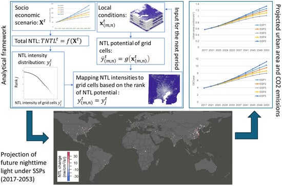
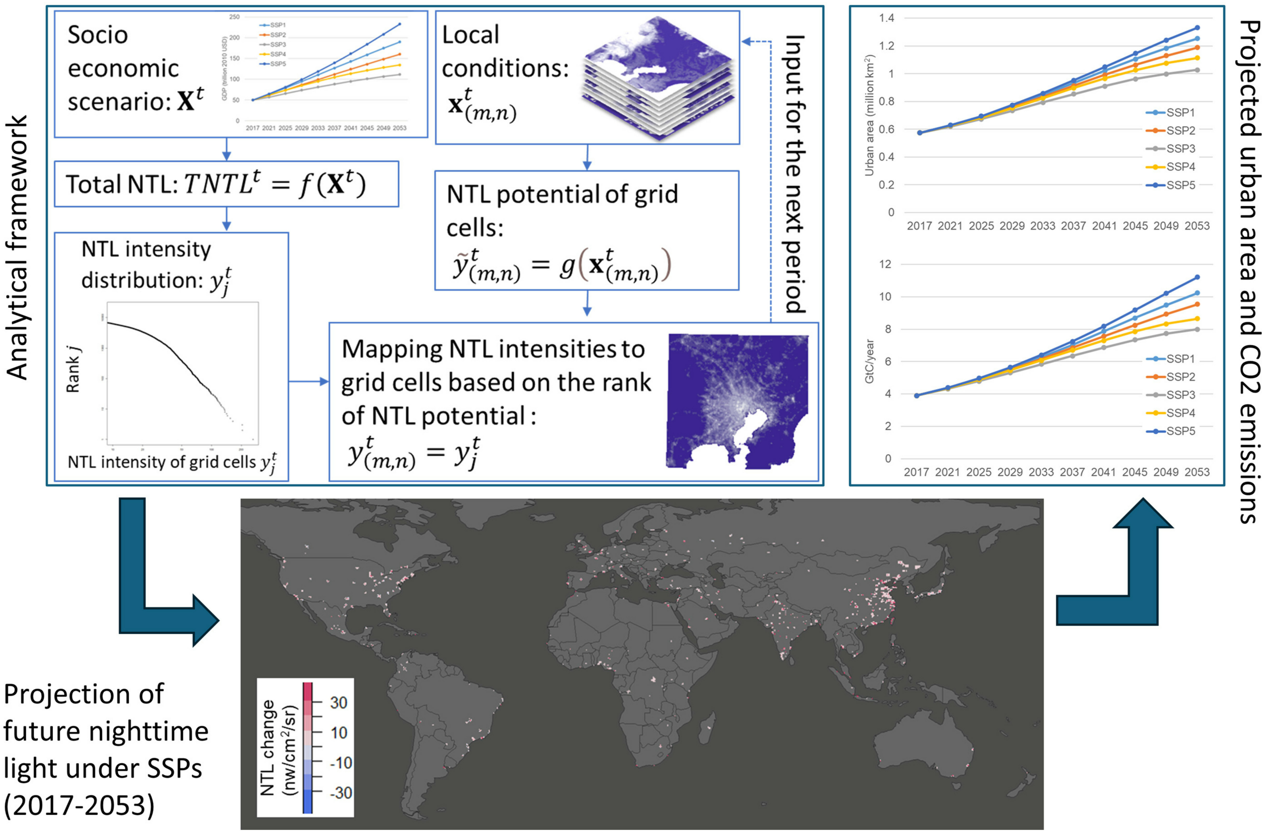
3.1. Conceptual Framework of Nighttime Light Scenario Generator

In this method, we set up the following steps to obtain a future scenario of grid-level nighttime light intensity:

(1)

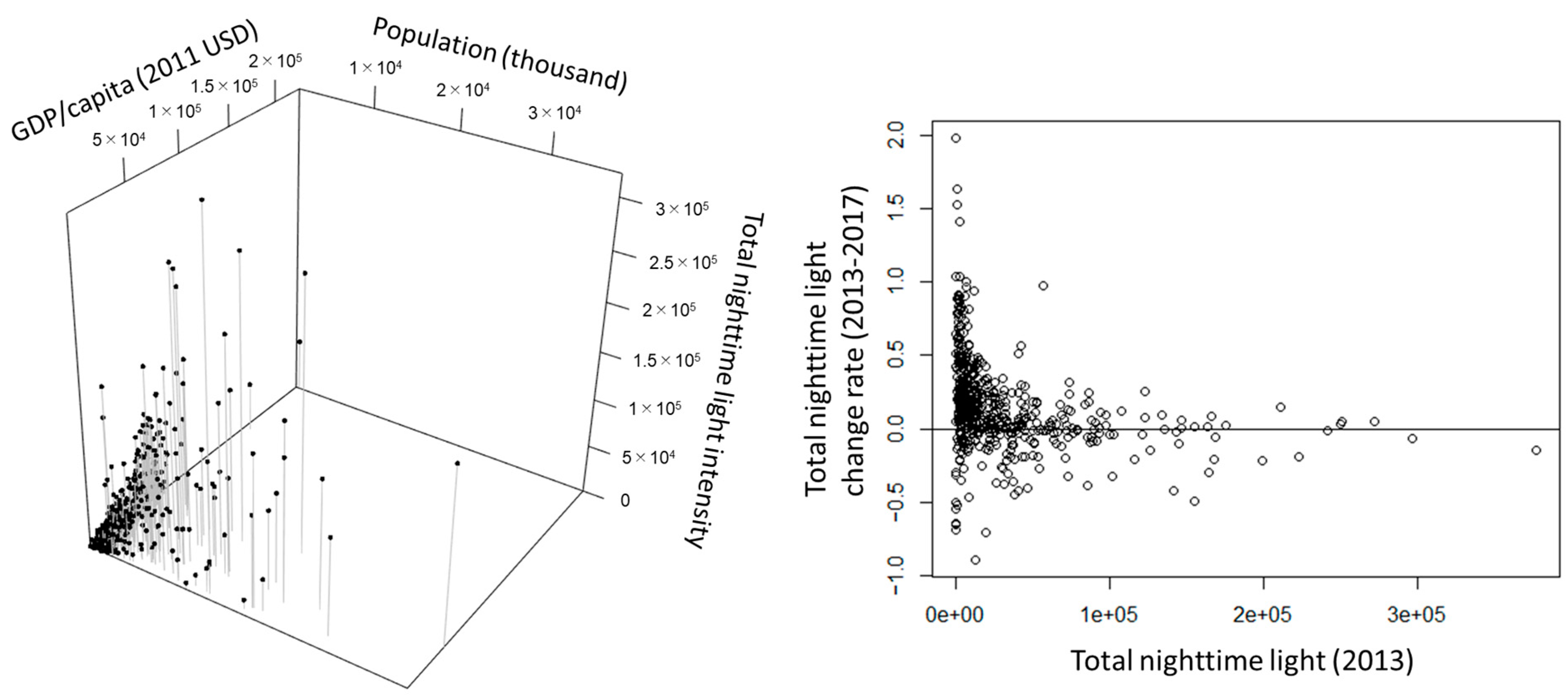
The total nighttime light intensity for urban areas is calculated based on socioeconomic indicators such as population and per capita GDP;

(2)

The intensity distribution of nighttime light that aligns with the calculated total nighttime light intensity is determined;

(3)

Grid-level nighttime light potentials are computed based on previous period nighttime light intensity, geographical conditions, and transportation conditions;

(4)

Nighttime light intensity is allocated from the highest values in the intensity distribution obtained in step 2 to grid cells based on the potentials derived in step 3, in descending order of intensity.

This process allows us to generate future scenarios that consider three conditions: the macro relationship between socioeconomic indicators and nighttime light, compliance with the empirical distribution of nighttime light intensity, and the influence of local conditions.

First, the total nighttime light intensity is known to have a strong correlation with socioeconomic indicators, as demonstrated in previous studies. When directly determining grid-level nighttime light intensity based on various geographical conditions, there is no guarantee that it will necessarily satisfy the macro-level relationship. Therefore, as a control total, the total nighttime light intensity for the entire urban area in period t ($TNT{L}^t$) is calculated using the following formula.

$$TNT{L}^t=f\left({\mathbf{X}}^t\right)$$

(1)

where, ${\mathbf{X}}^t$ represents the vector of socioeconomic indicators in period t, and $f$ is the function used to calculate the total nighttime light intensity. This equation will be concretized in Section 3.3. In this study, we assume a logarithmic linear function for $f$, and consider urban population and per capita GDP as ${\mathbf{X}}^t$.

Next, the vector of grid-specific nighttime light intensities arranged in descending order of their intensities is denoted as ${\mathbf{y}}^t=\left\{y_1^t,y_2^t,\dots ,y_J^t\right\}$ (where $y_{j-1}^t\le y_j^t, j=2,\dots ,J$), and an element is estimated by the following equation using the previous period’s nighttime light intensities and the total nighttime light intensity change:

$$y_j^t=y_j^{t-1}+\frac{y_j^{t-1}}{{\sum }_{j\in J}{y}_j^{t-1}}\left(TNT{L}^t-TNT{L}^{t-1}\right)$$

(2)

As a result, future estimates that preserve the intensity distribution of nighttime light can be obtained [42,43,44].

On the other hand, the individual grid cell’s nighttime light intensity potential is influenced not only by the previous nighttime light intensity but also by geographical conditions, transportation conditions, regulatory conditions, and other institutional factors. Denoting the local condition vector for grid cell (m, n) as ${\mathbf{x}}_{(m,n)}^t$, the nighttime light intensity potential ${\tilde{y}}_{\left(m,n\right)}^t$ for grid cell (m, n) is calculated using the following equation:

$${\tilde{y}}_{(m,n)}^t=g\left({\mathbf{x}}_{(m,n)}^t\right)$$

(3)

Here, $g$ will be specified in Section 3.3. In this study, we assume $g$ as a linear function. Additionally, ${\mathbf{x}}_{(m,n)}^t$ is assumed to include the previous period’s nighttime light intensity $\left\{y_{\left(m,n\right)}^{t-1}|\left(m,n\right)\in {\mathsf{\Omega }}_{TGC}\right\}$, where ${\mathsf{\Omega }}_{TGC}$ is the set of target grid cells.

Finally, when the rank of ${\tilde{y}}_{\left(m,n\right)}^t$ is j, the nighttime light intensity for grid cell $\left(m,n\right)$ is determined by $y_j^t$ calculated by Equation (2). This is expressed as follows:

$$j=rank\left({\tilde{y}}_{\left(m,n\right)}^t\right)=1+{\sum }_{{\left(m,n\right)}^{\prime }\in {\mathsf{\Omega }}_{TGC}}{\chi }_{{\tilde{y}}_{{\left(m,n\right)}^{\prime }}^t<{\tilde{y}}_{\left(m,n\right)}^t }$$

(4)

where, ${\chi }_{{\tilde{y}}_{j^{\prime }}^t<{\tilde{y}}_k^t }$ is an indicator function defined by the following equation.

$${\chi }_{{\tilde{y}}_{j^{\prime }}^t<{\tilde{y}}_{\left(m,n\right)}^t }=\left\{\begin{array}{c}1 if {\tilde{y}}_{j^{\prime }}^t<{\tilde{y}}_{\left(m,n\right)}^t\\ 0 else \end{array}\right.$$

(5)

With these formulae, $j$ expressed in Equation (4) is the rank of potential of nighttime light intensity ${\tilde{y}}_{\left(m,n\right)}^t$ in descending order.

As a result, the value of $y_j^t$ estimated by Equation (2) is mapped to $y_{\left(m,n\right)}^t$, which is the nighttime light intensity for grid cell $\left(m,n\right)$,

$$y_{\left(m,n\right)}^t=y_j^t$$

(6)

This procedure allows for the estimation of nighttime light intensity, taking into account both socioeconomic macro conditions and local/site-specific conditions. Here, the number of target grid cells $J$ in Equation (2) is equal to the number of grid cells used to estimate the potential in Equation (3), denoted as $\left|{\mathsf{\Omega }}_{TGC}\right|$. The mapping in Equation (6) is a one-to-one correspondence. Note that $\left\{{\tilde{y}}_{\left(m,n\right)}^t\right\}$ and $\left\{y_j^t\right\}$ may both contain elements with the same value, respectively. In such cases, for elements with the same value, random ranks are assigned within the range of their ranks. For example, if $n_r$ grids from $r_1$th to $\left(r_1+n_r-1\right)$th have the same nighttime light intensity or potential, random ranks from $r_1$th to $\left(r_1+n_r-1\right)$th are assigned to those grid cells. This randomness may lead to different results in calculation. However, since both nighttime light intensity and potential are real numbers, the likelihood of exactly the same value occurring in cells with high ranks is low. In addition, since the intensity distribution of nighttime light can be approximated by a Pareto distribution, the difference in intensity between ranks at lower ranks is expected to be small. Therefore, it is expected that the randomness will not have a significant impact on the results. Additionally, this study does not consider water surfaces, and thus, the set of target grid cells ${\mathsf{\Omega }}_{TGC}$ is a subset of urban grid cells. This process is illustrated in Figure 1.

3.2. Data

First, the target cities are selected from the United Nations World Urbanization Prospects (WUP) database (https://population.un.org/wup/, accessed on 1 July 2023), focusing on 555 cities with populations of 300,000 or more for which required data are available (Figure 2). The total population of the selected cities in 2015 was 1.65 billion, covering approximately 22.3% of the world’s total population.

As for socioeconomic data, population and per capita GDP are used. Population data were obtained from the aforementioned WUP database, while GDP was aggregated for each urban agglomeration based on grid-level GDP data provided by Kummu et al. [45]. However, the GDP data available in this dataset are in 2010 price-adjusted dollars using purchasing power parity (PPP) for the years 1990, 2000, and 2015. For years after 2015, changes in GDP per capita from the World Bank’s World Development Indicators (WDI) were applied.

Furthermore, for future scenarios, changes in both urban agglomeration populations and per capita GDP relative to current statistical values were set based on country-specific scenarios from the IIASA-SSP database [46]. Here, according to the narratives of SSPs [47], SSP1 describes a sustainable future and assumes fast urbanization in all countries, SSP2 is intermediate between other pathways with a moderate pace of urbanization, SSP3 assumes a regionalized world and slow urbanization, and SSP4 describes unequal, stratified economies with moderate urbanization in high-income countries and rapid urbanization in medium- and low-income countries. SSP5 describes rapid growth of the global economy and fast urbanization in all countries.

For estimating urban agglomeration populations, we followed the method outlined by Kii [48]. Additionally, for per capita GDP, we applied the country-specific change rates from the SSPs to the estimated values for each urban agglomeration obtained using the previously mentioned method.

As for nighttime light data, we utilized the annual median product of NPP-VIIRS [49]. Although NPP-VIIRS data have been available since 2012, it was only provided from April onwards, and there were significant data gaps in some cities. Therefore, we used data from 2013 onwards. As mentioned earlier, we used previous years’ nighttime light data as local conditions to determine grid-level nighttime light potential. In this case, we used 2013 data to estimate nighttime light for 2017. We also obtained the data for 2021, which will be used to validate the extrapolation of our model. Consequently, in the following section detailing the model specifics, we will use 2017 data for the base year. GDP and population figures are provided for the relevant years through linear interpolation.

As local conditions, we utilized the following factors: previous year’s nighttime light, travel time from the city center by road, distance from major roads, travel time from the city center by railway, distance from railway stations, water bodies, annual mean temperature, standard deviation of annual temperature, precipitation, standard deviation of precipitation, and the average and standard deviation of elevation and slope. Environmental protection areas were also included.

We derived travel time distances from the city center using road networks and railway networks from Openstreetmap. These network data were rasterized to create the necessary datasets. The distances from roads and railway stations were also based on rasterized data. The creation of distance data was performed using “R version 4.2.3” with the “gdistance package version 1.6”.

Water bodies data were obtained from the Terra Advanced Spaceborne Thermal Emission and Reflection Radiometer (ASTER) Global Water Bodies Database (ASTWBD) Version 1 (https://lpdaac.usgs.gov/products/astwbdv001/, accessed on 1 July 2023), while temperature and precipitation data came from WorldClim Version 2 (https://www.worldclim.com/version2 (1 July 2023)). Elevation and slope data were generated based on MERIT DEM (http://hydro.iis.u-tokyo.ac.jp/~yamadai/MERIT_DEM/, accessed on 1 July 2023). Information about environmental protection areas was sourced from the World Database on Protected Areas (https://www.protectedplanet.net/en, accessed on 1 July 2023).

3.3. Specification of the Model

In this section, we concretize the function $f$ for calculating the total nighttime light intensity, as shown in Equation (1), and the function $g$ for calculating the nighttime light potential of grid cells, as shown in Equation (3). First, we assume that the total nighttime light intensity for each city is explained by its population and per capita GDP. However, it can be observed from the data that the larger the total nighttime light intensity of the previous period, the smaller the rate of change in total nighttime light. Figure 3 on the left depicts a 3D plot of the total nighttime light intensity with respect to population and per capita GDP circa 2017, while Figure 3 on the right illustrates the rate of change in the total nighttime light intensity from 2013 to 2017 for each city, with respect to the total nighttime light intensity in 2013.

From this figure, it can be observed that there is a positive correlation between total nighttime light intensity and population, as well as GDP per capita. Additionally, it is evident that cities with lower total nighttime light intensity in 2013 tend to have a larger variance in the change rate from 2013 to 2017.

We assume a logarithmic-linear model for $f$ in Equation (1), which is expressed by the following equation.

$$ln\left(TNT{L}^t\right)={\alpha }_0+{\alpha }_{p}ln\left(Po{p}^t\right)+{\alpha }_{g}ln\left(GDP{p}^t\right)$$

(7)

Here, $Po{p}^t$ and $GDP{p}^p$ represent urban population and per capita GDP, respectively. The parameter estimation results are shown in

Table 1. Parameter estimation results of the nighttime light intensity model.

	Estimate	t Value
${\alpha }_0$	−6.289	−12.96
${\alpha }_p$	0.893	18.80
${\alpha }_g$	0.928	25.22
N	555
R2	0.663
F-statistic	542.1

. The estimation was conducted using cross-sectional data from 2017. As a result, all parameters are statistically significant. Although the R² is relatively low, it captures the trend that higher population and per capita GDP are associated with higher nighttime light intensity. With the availability of longer-term time series data, it may be possible to estimate city-specific fixed effects using panel data regression and improve the model. This is an area for potential enhancement as data accumulates in the future. There is room for improvement in the accuracy of nighttime light intensity estimation, but we utilize this model since we primarily focus on proposing a scenario generation method.

However, as we mentioned in the right panel of Figure 3, it is considered that the upper limit of the change rate of nighttime light may vary depending on the city size. That is, in small cities, it can change rapidly due to economic growth, but in large cities, it is presumed to have a smaller change rate. Here, we assumed a normal distribution for the change rate of nighttime light intensity from 2013 to 2017 and estimated a model under the assumption that its standard deviation is a function of nighttime light intensity in 2013. Specifically, we assumed that the standard deviation is given by the following formula:

$${\sigma }_i={\beta }_0+{\beta }_{1}exp\left({\beta }_{2}TNT{L}_i^{2013}\right)$$

(8)

Here, i is an index representing cities. We set the likelihood function for parameter estimation as follows:

$$LL={\sum }_i\left\{-\frac{1}{2}\ln \left(2\pi {\sigma }_i^2\right)-\frac{{\left((TNT{L}_i^{2017}-TNT{L}_i^{2013})/TNT{L}_i^{2013}-{\beta }_3\right)}^2}{2{\sigma }_i^2}\right\}$$

(9)

Table 2. Parameter estimation results of the standard deviation model.

	Estimate	t Value
${\beta }_0$	0.212	19.24
${\beta }_1$	0.510	5.30
${\beta }_2$	−3.64 × 10−4	−3.54
${\beta }_3$	0.109	8.43

shows the estimated parameters for the standard deviation model. From the fact that ${\beta }_2$ is less than 0, it can be inferred that as the total nighttime light increases, the standard deviation of the rate of change decreases. Furthermore, from the value of ${\beta }_0$, when the total nighttime light is sufficiently large, the standard deviation converges to around 0.2. Additionally, ${\beta }_3$ suggests an average increase of approximately 10% in the rate of change from 2013 to 2017. In this study, we assume the standard deviation as the upper limit of the rate of change and conduct simulations.

Next, we specify the function $g$ in Equation (3). Here, we created a linear regression model with the 2017 grid cell-level nighttime light as the dependent variable and explanatory variables including nighttime light for the same grid cell and the surrounding 8 grid cells in 2013, distances to the city center by road and railway, distance from roads, distance from railway stations, water surface dummy, temperature, precipitation, elevation, slope, average values and standard deviations of these variables, environmental protection area dummy, and urban area population and per capita GDP for the urban agglomeration. In the estimation, we used pooled data from all grid cells for all 555 cities, with approximately 2.56 million grid cells used for the estimation. We applied stepwise regression to the estimated model, selecting variables and excluding those that did not meet the plus/minus sign heuristics in urbanization. The estimation results are shown in

Table 3. Estimated parameters of the grid cell-specific nighttime light potential model.

	Model 1		Model 2		Model 3
Explanatory Variables 1	Estimate	t Value	Estimate	t Value	Estimate	t Value
(Intercept)	−1.29	−52.43	−1.29	−52.65	−0.705	−33.35
NTL.b	0.907	2687.30	0.907	2688.50	0.907	2691.25
RTC	−0.888	−114.02	−0.888	−114.24	−0.925	−124.47
RDD	−6.41 × 10−5	−48.51	−6.41 × 10−5	−48.75	−5.66 × 10−5	−43.44
TDS	2.76 × 10−2	18.92	2.76 × 10−2	18.91
PTC	−2.77 × 10−2	−18.95	−2.77 × 10−2	−18.94	−5.49 × 10−5	−32.58
WBD	1.66 × 10−3	0.08
TMP.a	0.155	205.38	0.155	205.79	0.140	226.77
TMP.v	8.31 × 10−4	55.69	8.31 × 10−4	55.70	5.13 × 10−4	40.15
PRC.a	−4.22 × 10−4	−71.83	−4.22 × 10−4	−71.86	−5.09 × 10−4	−95.50
PRC.v	−4.84 × 10−4	−4.98	−4.82 × 10−4	−4.96
talt.m	2.98 × 10−4	45.24	2.98 × 10−4	45.72
talt.sd	5.89 × 10−4	0.83
tslp.m	0.962	5.42	1.09	12.68
tslp.sd	−4.30	−20.14	−4.32	−20.35	−0.566	−6.71
PRC	−3.39 × 10−2	−3.28	−3.38 × 10−2	−3.28	−3.41 × 10−2	−3.32
NTL.fc.b	8.64 × 10−3	27.63	8.64 × 10−3	27.63	8.56 × 10−3	27.34
POP	4.37 × 10−5	84.89	4.37 × 10−5	84.94	4.48 × 10−5	87.38
GDPp	5.99 × 10−6	48.11	5.99 × 10−6	48.18	5.18 × 10−6	43.91
N	2,555,832
DF	2,555,813
R2	0.915		0.915		0.915

¹ NTL.b: previous period nighttime light; RTC: road travel time to city center; RDD: distance to road; TDS: distance to station; PTC: railway travel time to city center; WBD: waterbody dummy; TMP.a: annual mean temperature; TMP.v: standard deviation of monthly temperature; PRC.a: annual precipitation; PRC.v: standard deviation of monthly precipitation; talt.m: mean elevation; talt.sd: standard deviation of grid elevation; tslp.m: mean slope; tslp.sd: standard deviation of grid slope; PRC: protected area dummy; NTL.fc.b: average nighttime light intensity of surrounding 8 grid cells in the previous period; POP: current urban agglomeration population; GDPp: current urban agglomeration per capita GDP.

.

Here, Model 1 used all variables, Model 2 applied stepwise selection, and Model 3 further excluded variables that did not meet the heuristics. From this, in Model 1, the standard deviations of water surface and elevation were not significant and were excluded by the stepwise method. The parameter for distance to the railway station is positive, suggesting that the farther the railway station, the stronger the nighttime light. Also, the parameters for the average elevation and slope are positive. These parameters could potentially mislead future estimates, so these variables were excluded. The standard deviation of precipitation is negative, indicating that areas with less monthly precipitation variability have higher potential. However, it was excluded from the variables due to relatively low t-values. The R² values for these models are all 0.915, and it can be said that the reduction of variables has little impact on the current reproducibility. We will use Model 3 for the analyses below.

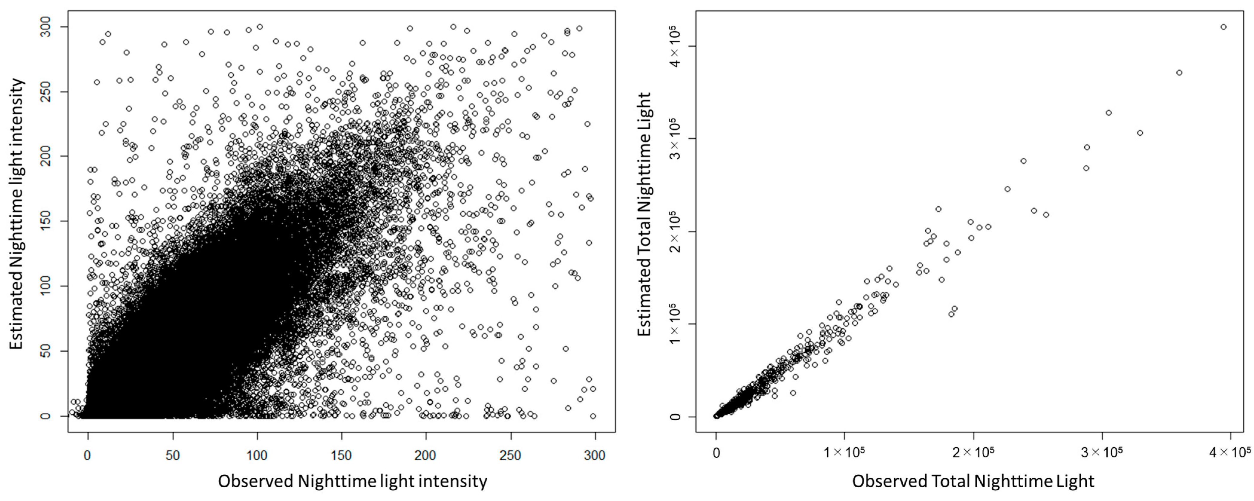
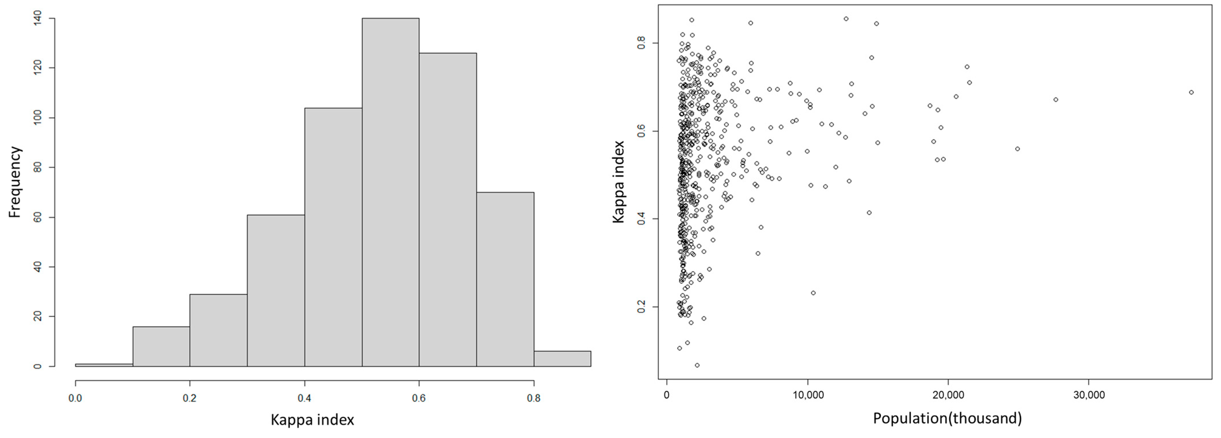
3.4. Model Validation

Here, we validated the estimation accuracy of the model by comparing the observational data of nighttime light intensity from 2021 with the estimated values generated using the model system. Assuming no significant differences between the Shared Socioeconomic Pathways (SSPs) in 2021, we used only SSP2 as the input condition for the estimation. Firstly, the multiple correlation coefficient between the estimated nighttime light intensity of approximately 2.56 million grid cells worldwide and the observed values was 0.54. Upon examining individual grids that have large errors, we observed certain grids emitting very strong nighttime light, which is presumed to be different from normal urban activities such as air defense. Therefore, when considering only grids with both observed and estimated values below 300 nW/cm²/sr for 2021, the multiple correlation coefficient increased to 0.87 (Figure 4, left). Furthermore, the multiple correlation coefficient between observed and estimated total nighttime light intensity aggregated for each of the 555 cities was 0.97 (Figure 4, right). This extrapolation of the model over a short period from 2017 to 2021 validates a certain level of estimation accuracy of our model. Additionally, it is evident that aggregating nighttime light intensity by city yields higher estimation accuracy compared to individual grid cells.

3.5. Estimation Model for Urban Areas and Carbon Emissions from Nighttime Light

We estimate the relationship to derive equations for estimating urban areas and carbon emissions from nighttime lights. For urban area estimation, similar to previous studies, we identify grid cells where nighttime lights exceed a certain threshold as urban areas. Here, we assume the European Space Agency (ESA), Climate Change Institute, Land Cover (CCI LC) time series data [50] as ground truth for urban land use and calculate the threshold, maximizing the following log-likelihood for each city from the 2017 nighttime lights:

$$\mathit{L}{\mathit{L}}_{\mathit{L}\mathit{C}}=\mathbf{ln}\left(\frac{{\mathit{n}}_{\mathbf{11}}}{{\mathit{n}}_{\mathbf{11}}+{\mathit{n}}_{\mathbf{12}}}\right)+\mathbf{ln}\left(\frac{{\mathit{n}}_{\mathbf{22}}}{{\mathit{n}}_{\mathbf{22}}+{\mathit{n}}_{\mathbf{21}}}\right)$$

(10)

where $n_{11}={\mathsf{\Omega }}_1\cap \widetilde{{\mathsf{\Omega }}_1}$, $n_{12}={\mathsf{\Omega }}_1\cap \widetilde{{\mathsf{\Omega }}_2}$, $n_{21}={\mathsf{\Omega }}_2\cap \widetilde{{\mathsf{\Omega }}_1}$, and $n_{22}={\mathsf{\Omega }}_2\cap \widetilde{{\mathsf{\Omega }}_2}$, ${\mathsf{\Omega }}_1$, ${\mathsf{\Omega }}_2$ are sets of urban and non-urban grid cells according to ESA CCI LC, $\widetilde{{\mathsf{\Omega }}_1}=\{\forall i|y_i\ge \mu \}$ and $\widetilde{{\mathsf{\Omega }}_2}=\{\forall i|y_i<\mu \}$ are estimated set of urban and non-urban grid cells, where $y_i$ represents nighttime light value, and $\mu$ is the threshold.

The left side of Figure 5 shows the distribution of the Kappa index, which represents the fitness of the estimation. It can be seen that even with a simple urban area determination using nighttime lights and a threshold, good fitness of 0.4 or higher is achieved in many cities.

The right side of the figure presents a plot of the Kappa index against urban population, revealing that cities with low Kappa indices tend to have smaller populations. In other words, for smaller cities, it may be challenging to accurately determine urban areas using only nighttime lights. On the other hand, for cities above a certain size of population, it can be concluded that high-fitness estimations are possible.

In estimating carbon emissions, a regression model with nighttime light as the explanatory variable is created. Here, the Open-Data Inventory for Anthropogenic Carbon dioxide (ODIAC) [51,52] was used as the carbon emissions data at the 1 km grid level. However, ODIAC also estimates emissions from point sources such as power plants. On the other hand, nighttime light is assumed to be a proxy for final demand in this study. Therefore, we assume that emissions from these point sources are distributed to grid cells without point sources in proportion to their emissions, and the modified grid-level emissions are used as the dependent variable. Grid cells containing point sources were identified as outliers for each city and were not used for parameter estimation. Here, the mean (m) and standard deviation (σ) of carbon emissions in areas with nighttime light intensities above 10 nW/cm²/sr were calculated, and grid cells exceeding m+4σ were identified as outliers. Linear regression and log-linear regression models were estimated as carbon emission models, and the results are shown in

Table 4. Estimated parameters of carbon emission models.

Linear Regression			Log-Linear Regression
	Estimate	t Value		Estimate	t Value
(Intercept)	438.1	312.5	(Intercept)	5.261	9200.6
ntl	117.3	1146.2	log (ntl)	0.830	2212.0
n	3,468,619		n	3,468,619
R2	0.275		R2	0.585
			R2~ntl	0.302

.

We can find that both models show a positive correlation between nighttime light and carbon emissions. Additionally, since grid-specific values are used and the sample size is sufficiently large, the parameters are statistically significant. Regarding reproducibility, the R² for the linear model is 0.275, while for the logarithmic model, it is 0.585. However, in the logarithmic model, the variables are correlated based on the logarithmically transformed values. The correlation coefficient for the transformed variables to original carbon emission is 0.302. Therefore, in terms of correlation, the logarithmic model appears to provide a better fit compared to the linear model. Consequently, the logarithmic model will be used in the subsequent analyses.

Furthermore, it should be noted that the logarithmic model indicates a diminishing rate of increase in carbon emissions in response to an increase in nighttime light intensity, as compared to the linear model. This interpretation suggests that it reflects an improvement in energy efficiency due to urban concentration. It is important to mention that ODIAC uses calibrated nighttime light based on DMSP-OLS for carbon emission estimation. Thus, in this study, carbon emissions estimated using nighttime light are essentially re-estimated using nighttime light again. We should interpret that the regression models used in this study capture correlations but not causality.

Moreover, in this research, nighttime light is assumed to be an aggregated proxy indicator for various human activities. Naturally, when examining individual grid cells, there will be errors in carbon emission estimation. However, at the urban agglomeration level, it is expected that these errors will be partially canceled out. In this study, a common carbon emission model is used for all cities worldwide. Therefore, an adjustment coefficient for each city was determined to ensure that the observed and estimated carbon emissions for each city matched in the base year, 2017. For the estimations under future scenarios, this coefficient is fixed and applied to each city.

4. Results

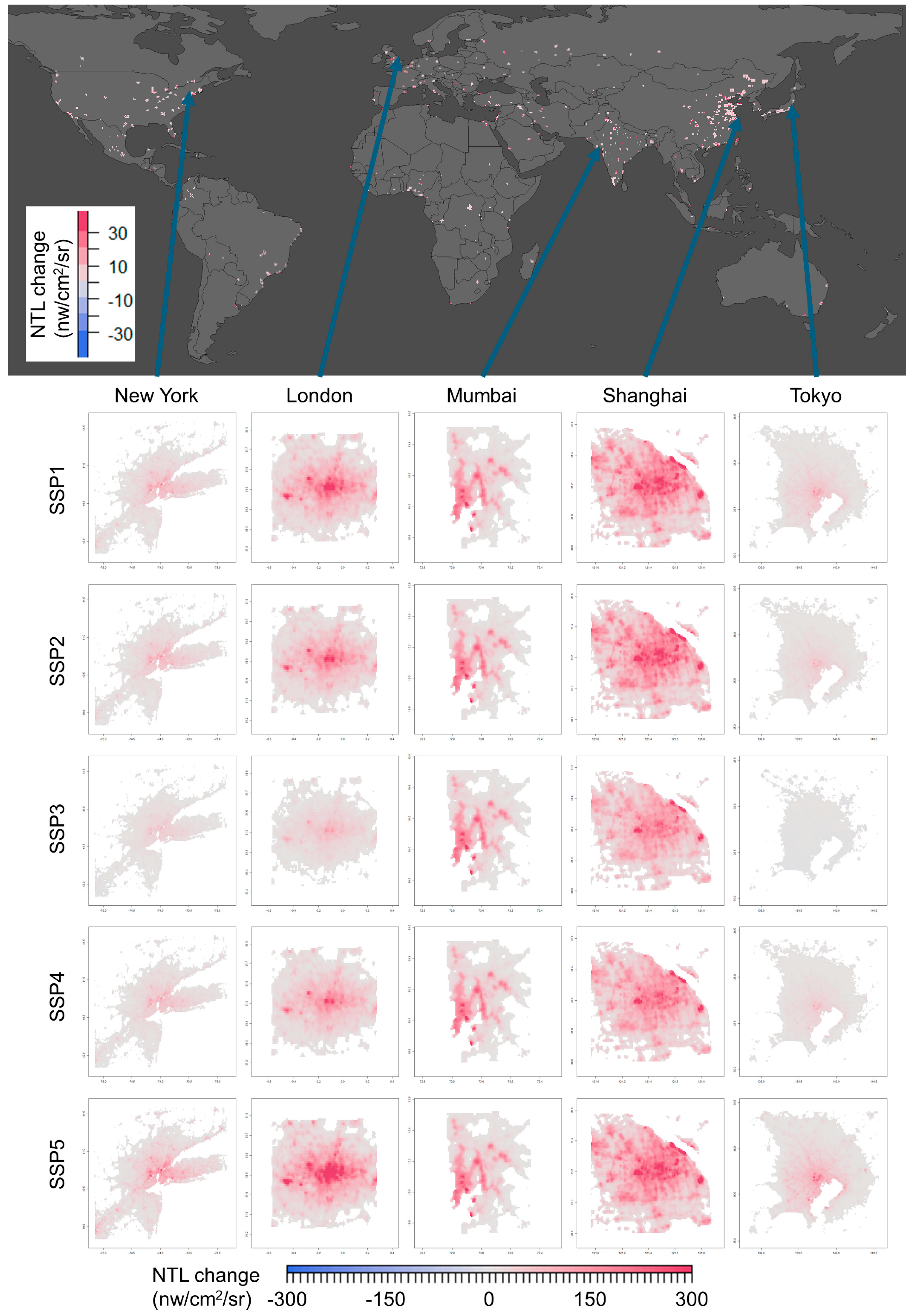
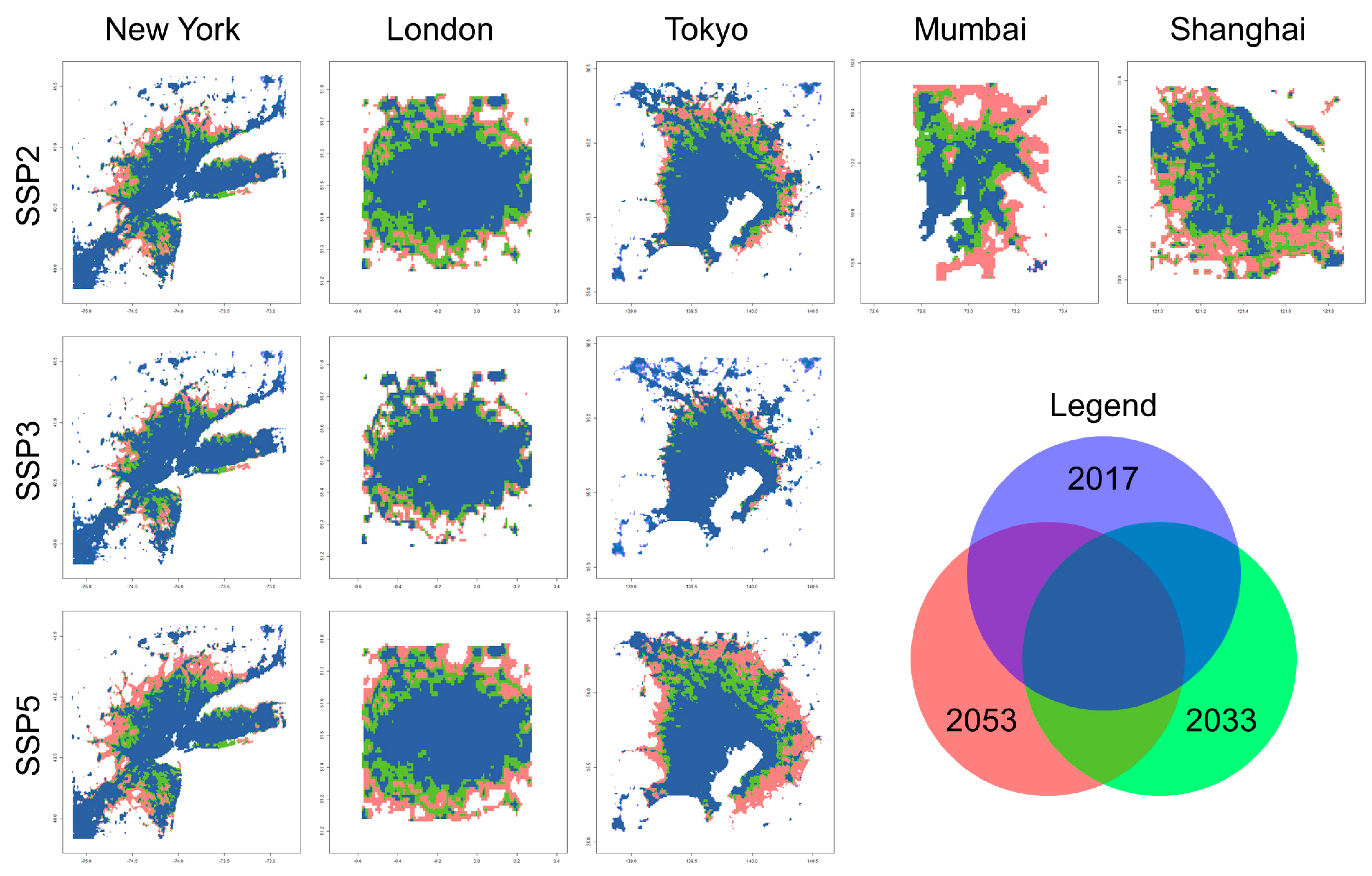
4.1. Nighttime Light Projection and Urban Area for Selected Cities

Using the above-mentioned method, we estimated nighttime lights for the 555 selected cities from 2017 to 2053. Figure 6 shows the changes in nighttime lights for all target cities in SSP2 from 2017 to 2053, as well as examples for Tokyo, Shanghai, Mumbai, London, and New York for each SSP1-5 during the same period. It is important to note that the world map shown represents changes in nighttime lights for the specific 555 cities, and it does not cover all regions.

When examining the city-specific estimation results, it becomes evident that nighttime light changes vary significantly depending on the SSP scenarios, especially in advanced countries’ cities. In Tokyo, London, and New York, SSP5 shows a substantial increase in nighttime lights, while SSP3 exhibits lower increases, with Tokyo experiencing almost no change. This difference can be attributed to the narrative that SSP5 anticipates rapid global economic growth and urbanization progress in all countries, leading to further urban activities, even in advanced-country cities. The absolute level of nighttime light estimated here varies by SSPs, as estimated in Equation (7). However, the SSPs do not affect the ranking of nighttime light intensity potential estimated by Model 3. This is because, in Model 3, the total population and average GDP per capita of urban areas are inputted, resulting in the same value being inputted for each cell within the urban area.

On the other hand, SSP3 assumes regional fragmentation and slower economic development globally, with higher population growth rates in developing countries and lower rates in advanced countries. Consequently, especially in advanced-country cities, lower nighttime light changes are estimated. In contrast, in developing-country cities, economic growth rates and population growth rates are higher compared to advanced countries, and the estimated total nighttime light levels reach the upper limit of the macro-level nighttime light change rates mentioned in Section 3.3 in many cases.

In Mumbai, all scenarios reach the upper limit, while in Shanghai, SSP1, 2, and 5 consistently reach the upper limit throughout the entire period, and even in SSP3 and SSP4, they reach the limit before 2045. As a result, for Mumbai, there are no significant differences in estimation results between scenarios, and for Shanghai, the differences remain minimal.

Next, Figure 7 presents the results of urban areas estimated using the method from Section 3.4. Here, we show the standard case as SSP2, the low-growth case as SSP3, and the high-growth case as SSP5. SSP1 and SSP4 represent intermediate cases and are omitted. Additionally, as previously mentioned, Mumbai and Shanghai have nearly identical estimated urban areas due to the upper limit constraints on the total nighttime light increase rate. Therefore, we only show the case for SSP2 for these two cities.

As a result, Mumbai and Shanghai exhibit significant increases in their urban areas. For Mumbai and Shanghai, it is estimated that their urban areas will increase by 56% and 49% in 2033 and 141% and 97% in 2053, respectively, compared to 2017. On the other hand, Tokyo, London, and New York show varying trends in urban area changes depending on the SSP scenarios. In SSP2, the urban areas of Tokyo, London, and New York in 2053 are estimated to increase by 36%, 61%, and 35%, respectively, compared to 2017. However, in SSP3, Tokyo is estimated to decrease by 2%, while London and New York are estimated to increase by 35% and 22%, respectively. In SSP5, they are estimated to increase by 70%, 75%, and 52%, respectively.

It is worth noting that in SSP3 for Tokyo, the peripheral urban areas are shrinking while the urban area is expanding at the boundary of the central cluster. This reflects the inclusion of the distance from the city center as a variable in the nightlight potential model (Equation (3)). Previous research has shown that ESA CCI LC identifies a broader area as urban than the official urban area definitions in Japan for the Tokyo metropolitan area [27]. In this study, ESA CCI LC was assumed as the true urban area, but it is important to note that the estimated results may vary depending on the urban area definition. Additionally, this study employs a globally consistent potential model and does not account for individual city’s land use regulations. Therefore, the estimated urban area results presented in this study should be regarded as areas with high development pressure based on potential. Whether these areas will be developed in the future or not will depend on the specific land use policies of individual cities. It is important to mention that this analysis model can flexibly estimate future scenarios at the grid level, so if spatial data on areas with development restrictions or other factors are available, it would be possible to incorporate them into scenario estimations.

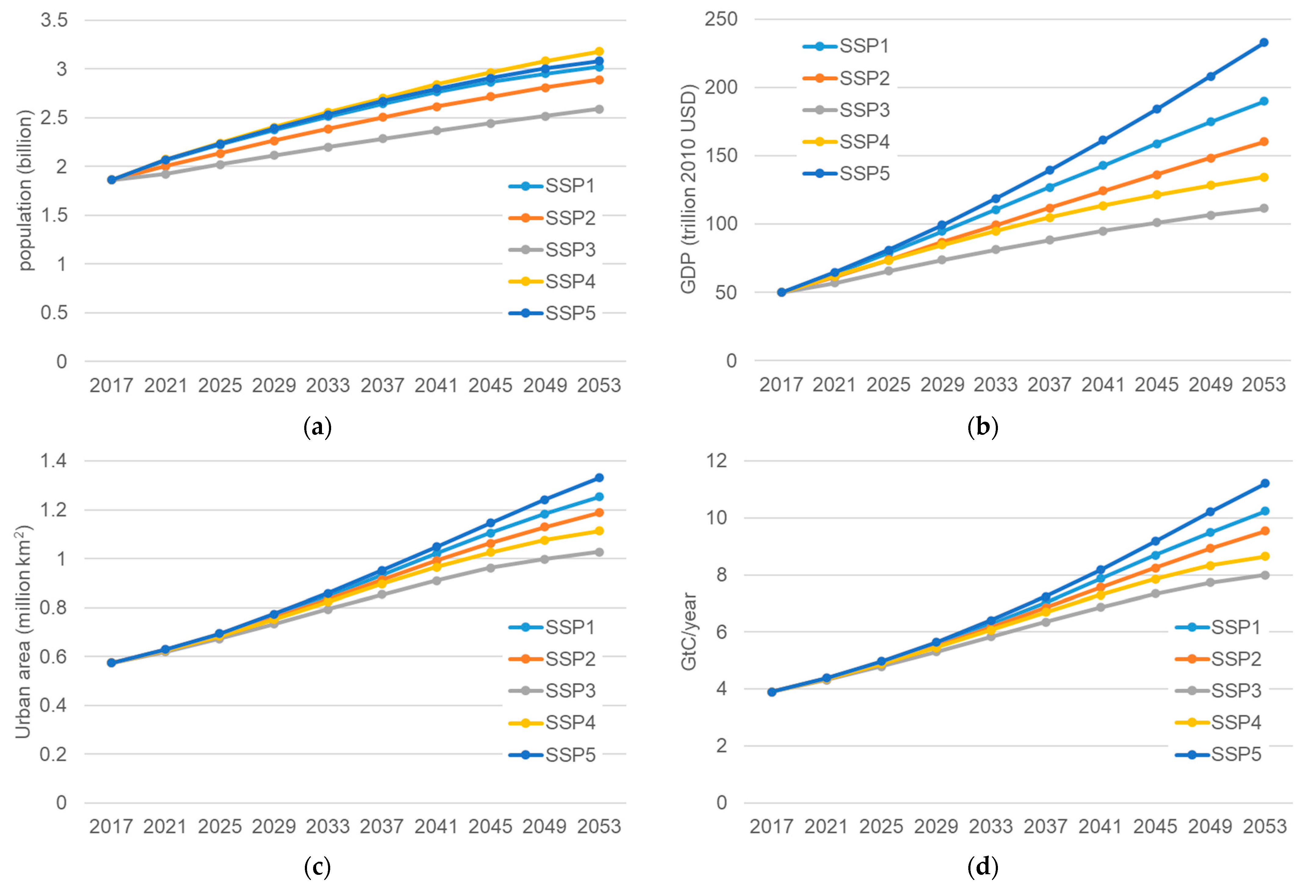
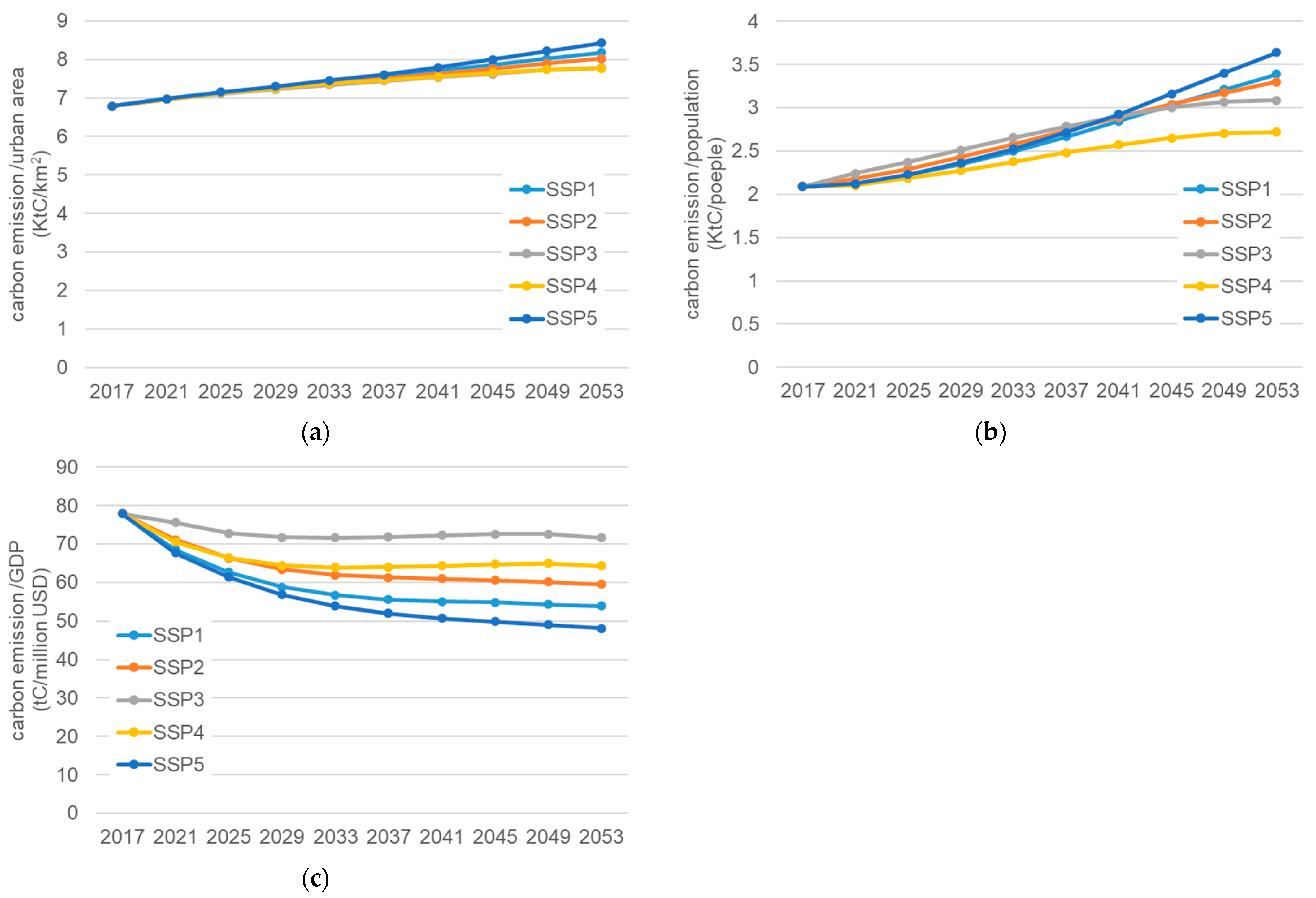
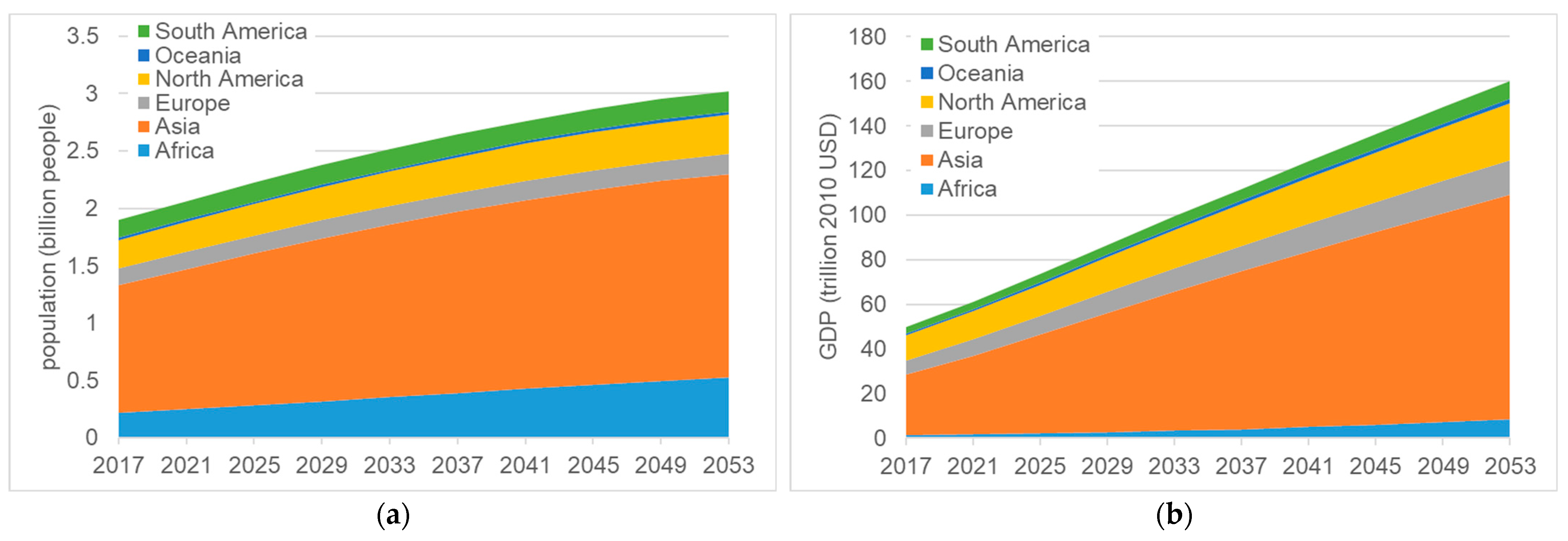
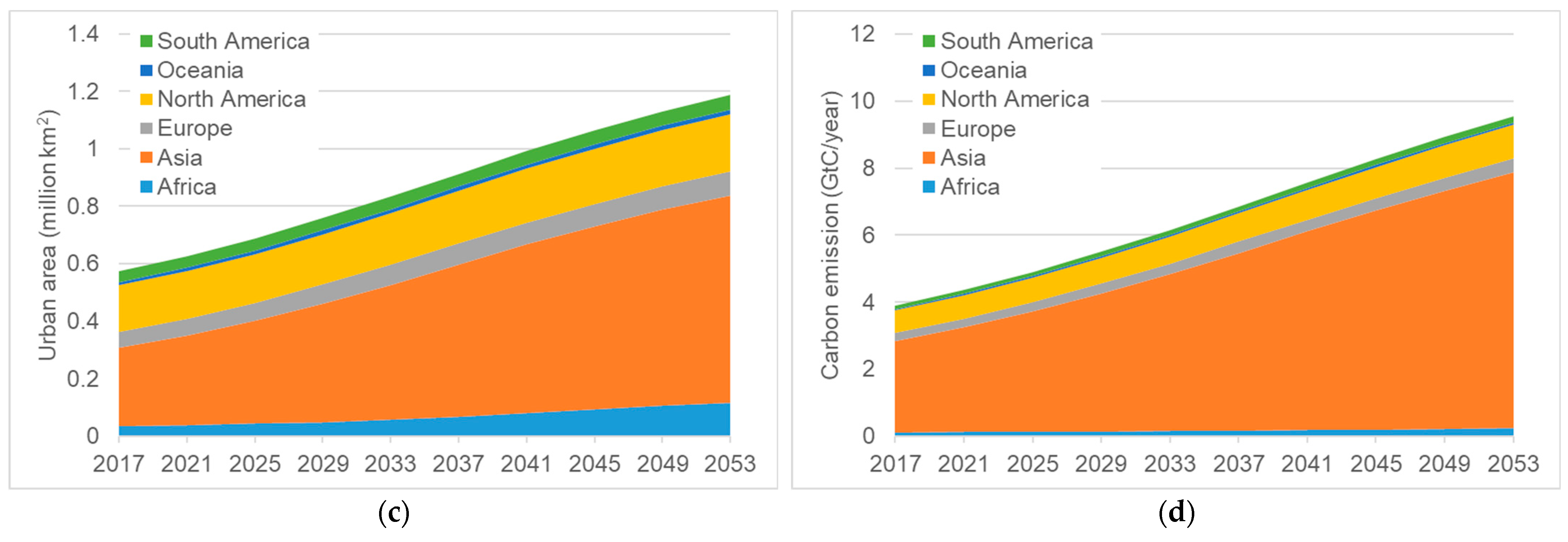
4.2. Estimated Urban Expansion and Carbon Emissions by SSPs

Figure 8 presents the estimated results of urban areas and carbon emissions for the 555 target cities worldwide, broken down by SSP-specific population, GDP scenarios, urban areas, and carbon emissions. Here, carbon emissions are estimated using the model presented in Table 4 and do not take into account emission reduction by decarbonization technologies. It is important to note that the changes in carbon emissions presented in this study are based solely on the observed correlation between nighttime light and CO₂ emissions, and the estimated CO₂ emissions are derived from the estimated nighttime light intensity.

Naturally, it is observed that in SSP3, which has the least population and GDP growth, urban areas and carbon emissions are estimated to be the lowest. On the other hand, in SSP4, which has the highest population growth but lower GDP growth, the increase in urban areas and carbon emissions is lower. Meanwhile, SSP5, with the highest GDP growth, exhibits the highest increase in urban areas and carbon emissions. From these observations, we can infer that GDP has a larger contribution to carbon emissions compared to population in this estimation.

It is worth noting that the carbon emissions estimated in this study for the year 2017 amount to 3.89 gigatonnes of carbon (GtC), equivalent to 44% of carbon emissions from energy sources in the same year. It should also be noted that the future carbon emissions estimates in this study are based solely on the current correlation with nighttime lights and do not take into account advancements in decarbonization technologies and other factors.

For validation of our estimate,

Table 5. Estimation of urban area changes in our study and previous studies.

Source	Period	Estimated Urban Area Increase
This study	2017 to 2053	79% to 132%
Huang et al. [16]	2015 to 2050	78% to 171%
Li et al. [17]	2013 to 2050	40% to 67%
Chen et al. [18]	2015 to 2100	53.8% to 110.6%
Gao and O’Neill [19]	2010 to 2050	51% to 168%
Zhou et al. [20]	2012 to 2050	About 40%

presents the estimated results of the urban area changes in previous studies worldwide, and the estimated results of the urban area changes in this study. However, it is important to note that this study focuses only on 555 cities and does not encompass all cities worldwide. Upon reviewing these results, it can be observed that our estimates fall within the range of estimates from previous studies.

We can find that from 2017 to 2053, urban areas have increased by approximately 1.8 to 2.3 times. Additionally, carbon emissions have increased by a factor of 2.1 to 2.9 during the same period. This reflects an increase in the density of urban activities. Furthermore, while the population has increased by a factor of 1.4 to 1.7, GDP has increased by a factor of 2.2 to 4.7. These observations indicate that while per capita carbon emissions are increasing, emissions per unit of GDP are decreasing. To illustrate this more clearly, Figure 9 displays the trends of carbon emissions concerning urban areas, population, and GDP.

From the figure, it is evident that carbon emissions per unit of urban area increase in all scenarios, with an increase of 1.1 to 1.2 times compared to 2017 by 2053. Similarly, per capita emissions also increase, ranging from 1.3 to 1.7 times. In contrast, emissions per unit of GDP decrease in all scenarios, ranging from 0.6 to 0.9 times. When looking at individual scenarios, SSP5 shows the highest emissions per capita and per unit of urban area, while SSP4 exhibits the lowest values. However, in terms of emissions per unit of GDP, SSP3 shows the smallest decrease, while SSP5 exhibits the largest decrease. SSP4 represents a scenario of societal fragmentation where the population increases significantly, but the growth rate of per capita GDP is the lowest, resulting in the lowest per capita carbon emissions. On the other hand, SSP3 has the smallest population and GDP in all scenarios, leading to the highest emissions per economic activity. SSP5, with the highest economic activity, has the highest per capita emissions but the lowest emissions per unit of GDP.

Figure 10 displays regional aggregates of urban area, population, GDP scenarios, and estimated carbon emissions for the 555 cities under SSP2. While the share of Asia is high in this scenario, it reflects the fact that many of the cities in this study are located in China and India. Therefore, it is important to note that these regional aggregates do not align with global, regional totals. The results suggest that carbon emissions are estimated to increase significantly in Asia by 2053. While Africa shows some growth in population and urban area, the impact on carbon emissions is not significant during the study period.

5. Discussion

5.1. Features of the Nighttime Light Estimation Method

The distinctive features of our method lie in the proposal of an analytical framework that estimates the total nighttime light using a macro model, derives the intensity distribution of nighttime light from it, and allocates it based on grid-specific potentials. This framework enables the estimation of the spatial distribution of nighttime light that reflects both macro conditions and the empirical rules of nighttime light intensity distribution while also taking into account local conditions. This allows for a coherent estimation that considers both macro and micro conditions. Moreover, by breaking down the estimation into modules, it becomes easier to incorporate improvements in each module into the system. For instance, we estimate city-specific total nighttime light using a simple global model with population and per capita GDP as explanatory variables. However, it is possible to replace this with more sophisticated models using panel data and other advanced approaches. Similarly, for potential estimation models that consider local conditions, it is possible to replace them with spatial economic models, land use models, cellular automata models, and others. The key enabling factor here is the fitting process of estimated total nighttime light to the grid cells using empirical distribution functions and indicator functions, which is the original idea of this study.

5.2. Estimation of Urban Areas and Carbon Emissions

In this paper, we estimated nighttime light for 555 cities and predicted future urban expansion and changes in carbon emissions for each SSP scenario. Consequently, for all scenarios, it was estimated that both urban areas and carbon emissions would increase for the entire set of target cities. However, carbon emissions were projected to increase at a higher rate than urban areas, indicating an increase in the density of urban activities.

On the other hand, when examining individual cities, our method has the ability to analyze the diverse impacts of each scenario on different cities. For instance, in the SSP3 scenario, a contraction of urban areas was estimated for Tokyo, which exhibits a different morphological pattern compared to other cities.

It should be noted that in this study, policies such as the introduction of decarbonization technologies and urban land use control are not considered. Our estimation is based solely on the observed correlation between nighttime light and CO₂ emissions and future population and GDP scenarios. In this study, nighttime light intensity is assumed as a proxy indicator of human activity, and activity levels are estimated to increase from future population and GDP under the Shared Socioeconomic Pathways (SSPs). The implication of these results is the necessity for significantly increased implementation of urban policies and decarbonization technologies that contribute to CO₂ emission reduction in response to the expected intensification of human activity in the future for climate change mitigation. Otherwise, CO₂ emissions are projected to increase substantially.

It should also be noted that our method can be applicable to the analysis of the effects of various macro and local conditions. For instance, changes in urban population induced by national land planning and variations in economic activity levels represented by GDP can influence changes in nighttime light. Additionally, the impact of infrastructure development, such as roads and railways, on the spatial distribution of nighttime light can also be analyzed. While this study directly calculates future carbon emissions from nighttime light based on the statistical relationship between nighttime light intensity and carbon emissions, it is also conceivable to estimate carbon emissions based on the spatial distribution of urban activities assumed from nighttime light by estimating building quantities constructed and traffic volumes. Such processes could potentially enable a more wide range of climate and urban policy analyses.

Furthermore, in this study, the ESA CCI LC is used as the ground truth for urban areas, and the threshold for distinguishing urban areas is determined based on these data. As mentioned in Section 4.1, there is a possibility that the definition of urban areas varies depending on the region, which could also affect the results. Therefore, different results may be obtained due to changes in the reference data or definition of urban areas. Additionally, this paper aggregated data from Kummu et al. [45] for urban area GDP, but new data, such as that from Wang et al. [30], have also been released. When using different data sources, it is important to note that the results may also differ.

Furthermore, this study used UN-WUP data as the basis for defining urban areas, but it should be noted that some cities within these data can be considered part of the same urban area. Kii [47] proposed a method for determining whether cities listed in UN-WUP belong to the same urban area, and it may be necessary to establish comparable urban areas based on such criteria.

5.3. Limitations and Future Study

This study proposes a new method for predicting future nighttime light patterns, but it has several limitations. The models used for estimating nighttime light intensity by total light emissions and grid-specific light intensity potential could be improved in accuracy and validity by employing more sophisticated models. Additionally, we assume that the shape of the nighttime light distribution remains unchanged based on observed data, and we have not explored scenario generation methods that could alter this assumption. Furthermore, energy-saving and decarbonization technologies are held constant in the current analysis. To address these limitations, further research is needed to investigate the relationship between nighttime light and carbon emissions, as well as to disaggregate nighttime light into various activities and study the effects of technology on carbon emission efficiency. Additionally, the cities covered in this study represent only around 22% of the total global population as of 2015, so collecting and organizing data to scale up to the global urban area is necessary.

In addition, the technological progress in outdoor lighting used at night must be considered. In several countries, the replacement of sodium discharge lamps with LEDs for outdoor lighting is being promoted from an energy efficiency perspective. However, the impact of this transition on the nighttime light intensity observed by VIIRS has not been thoroughly evaluated. LEDs have a wide range of wavelengths, which may increase visibility with less light, potentially resulting in darker nighttime light. On the other hand, with the increased conversion efficiency of electrical energy to light, there is also the possibility of utilizing brighter light. Therefore, when using new nighttime light observation data, the relationship between socioeconomic indicators and CO₂ emissions needs to be calibrated on a case-by-case basis.

6. Conclusions

In this study, we propose a method for future nighttime light estimation and apply it to the SSP scenarios, estimating the spatial distribution of nighttime light until 2053 for 555 cities worldwide where data are available. Additionally, we estimate future urban areas and carbon emissions based on future nighttime light estimations and their relationships with urban land use and carbon emissions.

The analytical framework we propose allows for the integrated consideration of both the overall socioeconomic conditions and local conditions of urban areas. Moreover, this framework is flexible, making it easy to incorporate updates to data and improvements in component models into the analysis.

When applying this analytical framework to estimate the activities of 555 cities worldwide until 2053, we observed a substantial increase in urban land area and CO₂ emissions despite the latter not incorporating carbon emission reduction technologies. While this assumption may lead to biased results, it clearly highlights the spatial aspect of the impact of urban activities. On the other hand, future estimates of urban land use areas generally fall within the range of estimates from previous studies.

The new method proposed in this study is, therefore, flexible and straightforward for future estimation of urban activities using nighttime light. Additionally, the future estimation results can be reasonably valid compared to previous research. Of course, there is still room for improvement in the estimation methods for total nighttime light and grid cell-level potential. However, by upgrading these methods, the proposed framework can be applied to various socioeconomic scenarios to assess climate change impacts and analyze the effects on urban activities, such as urban infrastructure development and land use policies, thus enabling a more diverse range of applications. In the future, we plan to expand our research by increasing the number of target cities and population coverage and applying it to evaluations of climate change mitigation measures.

References

1. Krayenhoff, E.S.; Moustaoui, M.; Broadbent, A.M.; Gupta, V.; Georgescu, M. Diurnal interaction between urban expansion, climate change and adaptation in US cities. Nat. Clim. Change 2018, 8, 1097–1103. [Google Scholar] [CrossRef]
2. Liu, F.; Zhang, Z.; Zhao, X.; Wang, X.; Zuo, L.; Wen, Q.; Yi, L.; Xu, J.; Hu, S.; Liu, B. Chinese cropland losses due to urban expansion in the past four decades. Sci. Total Environ. 2019, 650, 847–857. [Google Scholar] [CrossRef]
3. Liu, Z.; He, C.; Wu, J. The Relationship between Habitat Loss and Fragmentation during Urbanization: An Empirical Evaluation from 16 World Cities. PLoS ONE 2016, 11, e0154613. [Google Scholar] [CrossRef] [PubMed]
4. McDonald, R.I.; Mansur, A.V.; Ascensão, F.; Colbert, M.l.; Crossman, K.; Elmqvist, T.; Gonzalez, A.; Güneralp, B.; Haase, D.; Hamann, M.; et al. Research gaps in knowledge of the impact of urban growth on biodiversity. Nat. Sustain. 2019, 3, 16–24. [Google Scholar] [CrossRef]
5. Pandey, R.; Alatalo, J.M.; Thapliyal, K.; Chauhan, S.; Archie, K.M.; Gupta, A.K.; Jha, S.K.; Kumar, M. Climate change vulnerability in urban slum communities: Investigating household adaptation and decision-making capacity in the Indian Himalaya. Ecol. Indic. 2018, 90, 379–391. [Google Scholar] [CrossRef]
6. van Vliet, J. Direct and indirect loss of natural area from urban expansion. Nat. Sustain. 2019, 2, 755–763. [Google Scholar] [CrossRef]
7. Zhang, H.; Wu, C.; Chen, W.; Huang, G. Effect of urban expansion on summer rainfall in the Pearl River Delta, South China. J. Hydrol. 2019, 568, 747–757. [Google Scholar] [CrossRef]
8. Baur, A.H.; Förster, M.; Kleinschmit, B. The spatial dimension of urban greenhouse gas emissions: Analyzing the influence of spatial structures and LULC patterns in European cities. Landsc. Ecol. 2015, 30, 1195–1205. [Google Scholar] [CrossRef]
9. Gudipudi, R.; Fluschnik, T.; Ros, A.G.C.; Walther, C.; Kropp, J.P. City density and CO2 efficiency. Energy Policy 2016, 91, 352–361. [Google Scholar] [CrossRef]
10. Jones, C.; Kammen, D.M. Spatial distribution of U.S. household carbon footprints reveals suburbanization undermines greenhouse gas benefits of urban population density. Environ. Sci. Technol. 2014, 48, 895–902. [Google Scholar] [CrossRef]
11. Lee, S.; Lee, B. Comparing the impacts of local land use and urban spatial structure on household VMT and GHG emissions. J. Transp. Geogr. 2020, 84, 102694. [Google Scholar] [CrossRef]
12. Wang, M.; Madden, M.; Liu, X. Exploring the Relationship between Urban Forms and CO2 Emissions in 104 Chinese Cities. J. Urban Plan. Dev. 2017, 143, 04017014. [Google Scholar] [CrossRef]
13. Lwasa, S.; Seto, K.C.; Bai, X.; Blanco, H.; Gurney, K.R.; Kılkış, Ş.; Lucon, O.; Murakami, J.; Pan, J.; Sharifi, A.; et al. Urban Systems and Other Settlements. In Climate Change 2022—Mitigation of Climate Change; Shukla, P.R., Skea, J., Slade, R., Al Khourdajie, A., van Diemen, R., McCollum, D., Pathak, M., Some, S., Vyas, P., Fradera, R., et al., Eds.; Cambridge University Press: Cambridge, UK; New York, NY, USA, 2023; pp. 861–952. [Google Scholar]
14. Croft, T.A. Nighttime Images of the Earth from Space. Sci. Am. 1978, 239, 86–98. [Google Scholar] [CrossRef]
15. Miller, S.D.; Mills, S.P.; Elvidge, C.D.; Lindsey, D.T.; Lee, T.F.; Hawkins, J.D. Suomi satellite brings to light a unique frontier of nighttime environmental sensing capabilities. Proc. Natl. Acad. Sci. USA 2012, 109, 15706–15711. [Google Scholar] [CrossRef] [PubMed]
16. Huang, K.; Li, X.; Liu, X.; Seto, K.C. Projecting global urban land expansion and heat island intensification through 2050. Environ. Res. Lett. 2019, 14, 114037. [Google Scholar] [CrossRef]
17. Li, X.; Zhou, Y.; Eom, J.; Yu, S.; Asrar, G.R. Projecting Global Urban Area Growth Through 2100 Based on Historical Time Series Data and Future Shared Socioeconomic Pathways. Earth’s Future 2019, 7, 351–362. [Google Scholar] [CrossRef]
18. Chen, G.; Li, X.; Liu, X.; Chen, Y.; Liang, X.; Leng, J.; Xu, X.; Liao, W.; Qiu, Y.; Wu, Q.; et al. Global projections of future urban land expansion under shared socioeconomic pathways. Nat. Commun. 2020, 11, 537. [Google Scholar] [CrossRef]
19. Gao, J.; O’Neill, B.C. Mapping global urban land for the 21st century with data-driven simulations and Shared Socioeconomic Pathways. Nat. Commun. 2020, 11, 2302. [Google Scholar] [CrossRef]
20. Zhou, Y.; Varquez, A.C.G.; Kanda, M. High-resolution global urban growth projection based on multiple applications of the SLEUTH urban growth model. Sci. Data 2019, 6, 34. [Google Scholar] [CrossRef]
21. Zhou, Y.; Li, X.; Asrar, G.R.; Smith, S.J.; Imhoff, M. A global record of annual urban dynamics (1992–2013) from nighttime lights. Remote Sens. Environ. 2018, 219, 206–220. [Google Scholar] [CrossRef]
22. Seto, K.C.; Fragkias, M.; Guneralp, B.; Reilly, M.K. A meta-analysis of global urban land expansion. PLoS ONE 2011, 6, e23777. [Google Scholar] [CrossRef] [PubMed]
23. Guneralp, B.; Zhou, Y.; Urge-Vorsatz, D.; Gupta, M.; Yu, S.; Patel, P.L.; Fragkias, M.; Li, X.; Seto, K.C. Global scenarios of urban density and its impacts on building energy use through 2050. Proc. Natl. Acad. Sci. USA 2017, 114, 8945–8950. [Google Scholar] [CrossRef] [PubMed]
24. Große, J.; Fertner, C.; Groth, N.B. Urban Structure, Energy and Planning: Findings from Three Cities in Sweden, Finland and Estonia. Urban Plan. 2016, 1, 24–40. [Google Scholar] [CrossRef]
25. Mahtta, R.; Mahendra, A.; Seto, K.C. Building up or spreading out? Typologies of urban growth across 478 cities of 1 million+. Environ. Res. Lett. 2019, 14, 124077. [Google Scholar] [CrossRef]
26. Chen, Z.; Yu, B.; Song, W.; Liu, H.; Wu, Q.; Shi, K.; Wu, J. A New Approach for Detecting Urban Centers and Their Spatial Structure with Nighttime Light Remote Sensing. IEEE Trans. Geosci. Remote Sens. 2017, 55, 6305–6319. [Google Scholar] [CrossRef]
27. Kii, M.; Tamaki, T.; Suzuki, T.; Nonomura, A. Estimating urban spatial structure based on remote sensing data. Sci. Rep. 2023, 13, 8804. [Google Scholar] [CrossRef] [PubMed]
28. Li, X.; Xu, H.; Chen, X.; Li, C. Potential of NPP-VIIRS Nighttime Light Imagery for Modeling the Regional Economy of China. Remote Sens. 2013, 5, 3057–3081. [Google Scholar] [CrossRef]
29. Shi, K.; Yu, B.; Huang, Y.; Hu, Y.; Yin, B.; Chen, Z.; Chen, L.; Wu, J. Evaluating the Ability of NPP-VIIRS Nighttime Light Data to Estimate the Gross Domestic Product and the Electric Power Consumption of China at Multiple Scales: A Comparison with DMSP-OLS Data. Remote Sens. 2014, 6, 1705–1724. [Google Scholar] [CrossRef]
30. Wang, X.; Sutton, P.C.; Qi, B. Global Mapping of GDP at 1 km2 Using VIIRS Nighttime Satellite Imagery. ISPRS Int. J. Geo-Inf. 2019, 8, 580. [Google Scholar] [CrossRef]
31. Shi, K.; Chen, Y.; Yu, B.; Xu, T.; Chen, Z.; Liu, R.; Li, L.; Wu, J. Modeling spatiotemporal CO2 (carbon dioxide) emission dynamics in China from DMSP-OLS nighttime stable light data using panel data analysis. Appl. Energy 2016, 168, 523–533. [Google Scholar] [CrossRef]
32. Letu, H.; Nakajima, T.Y.; Nishio, F. Regional-Scale Estimation of Electric Power and Power Plant CO2 Emissions Using Defense Meteorological Satellite Program Operational Linescan System Nighttime Satellite Data. Environ. Sci. Technol. Lett. 2014, 1, 259–265. [Google Scholar] [CrossRef]
33. Zhang, X.; Xie, Y.; Jiao, J.; Zhu, W.; Guo, Z.; Cao, X.; Liu, J.; Xi, G.; Wei, W. How to accurately assess the spatial distribution of energy CO2 emissions? Based on POI and NPP-VIIRS comparison. J. Clean. Prod. 2023, 402, 136656. [Google Scholar] [CrossRef]
34. Zhou, L.; Song, J.; Chi, Y.; Yu, Q. Differential Spatiotemporal Patterns of CO2 Emissions in Eastern China’s Urban Agglomerations from NPP/VIIRS Nighttime Light Data Based on a Neural Network Algorithm. Remote Sens. 2023, 15, 404. [Google Scholar] [CrossRef]
35. Yang, J.; Li, W.; Chen, J.; Sun, C. Refined Carbon Emission Measurement Based on NPP-VIIRS Nighttime Light Data: A Case Study of the Pearl River Delta Region, China. Sensors 2022, 23, 191. [Google Scholar] [CrossRef]
36. Ou, J.; Liu, X.; Li, X.; Li, M.; Li, W. Evaluation of NPP-VIIRS Nighttime Light Data for Mapping Global Fossil Fuel Combustion CO2 Emissions: A Comparison with DMSP-OLS Nighttime Light Data. PLoS ONE 2015, 10, e0138310. [Google Scholar] [CrossRef] [PubMed]
37. Chen, H.; Zhang, X.; Wu, R.; Cai, T. Revisiting the environmental Kuznets curve for city-level CO2 emissions: Based on corrected NPP-VIIRS nighttime light data in China. J. Clean. Prod. 2020, 268, 121575. [Google Scholar] [CrossRef]
38. Small, C.; Pozzi, F.; Elvidge, C. Spatial analysis of global urban extent from DMSP-OLS night lights. Remote Sens. Environ. 2005, 96, 277–291. [Google Scholar] [CrossRef]
39. Zhu, J.; Lang, Z.; Wang, S.; Zhu, M.; Na, J.; Zheng, J. Using Dual Spatial Clustering Models for Urban Fringe Areas Extraction Based on Night-time Light Data: Comparison of NPP/VIIRS, Luojia 1-01, and NASA’s Black Marble. ISPRS Int. J. Geo-Inf. 2023, 12, 408. [Google Scholar] [CrossRef]
40. Wu, B.; Huang, H.; Wang, Y.; Shi, S.; Wu, J.; Yu, B. Global spatial patterns between nighttime light intensity and urban building morphology. Int. J. Appl. Earth Obs. Geoinf. 2023, 124, 103495. [Google Scholar] [CrossRef]
41. Kii, M.; Matsumoto, K. Detecting Urban Sprawl through Nighttime Light Changes. Sustainability 2023, 15, 16506. [Google Scholar] [CrossRef]
42. Albert, R.; Barabási, A.-L. Statistical mechanics of complex networks. Rev. Mod. Phys. 2002, 74, 47–97. [Google Scholar] [CrossRef]
43. Barabasi, A.L.; Albert, R. Emergence of scaling in random networks. Science 1999, 286, 509–512. [Google Scholar] [CrossRef]
44. Kii, M.; Akimoto, K.; Doi, K. Random-growth urban model with geographical fitness. Phys. A: Stat. Mech. Its Appl. 2012, 391, 5960–5970. [Google Scholar] [CrossRef]
45. Kummu, M.; Taka, M.; Guillaume, J.H.A. Gridded global datasets for Gross Domestic Product and Human Development Index over 1990–2015. Sci. Data 2018, 5, 180004. [Google Scholar] [CrossRef]
46. Riahi, K.; van Vuuren, D.P.; Kriegler, E.; Edmonds, J.; O’Neill, B.C.; Fujimori, S.; Bauer, N.; Calvin, K.; Dellink, R.; Fricko, O.; et al. The Shared Socioeconomic Pathways and their energy, land use, and greenhouse gas emissions implications: An overview. Glob. Environ. Change 2017, 42, 153–168. [Google Scholar] [CrossRef]
47. O’Neill, B.C.; Kriegler, E.; Ebi, K.L.; Kemp-Benedict, E.; Riahi, K.; Rothman, D.S.; van Ruijven, B.J.; van Vuuren, D.P.; Birkmann, J.; Kok, K.; et al. The roads ahead: Narratives for shared socioeconomic pathways describing world futures in the 21st century. Glob. Environ. Change 2017, 42, 169–180. [Google Scholar] [CrossRef]
48. Kii, M. Projecting future populations of urban agglomerations around the world and through the 21st century. NPJ Urban. Sustain. 2021, 1, 10. [Google Scholar] [CrossRef]
49. Elvidge, C.D.; Zhizhin, M.; Ghosh, T.; Hsu, F.-C.; Taneja, J. Annual Time Series of Global VIIRS Nighttime Lights Derived from Monthly Averages: 2012 to 2019. Remote Sens. 2021, 13, 922. [Google Scholar] [CrossRef]
50. ESA. Land Cover CCI Product User Guide Version 2; European Space Agency: Brussels, Belgium, 2017; p. 105.
51. Oda, T.; Maksyutov, S. A very high-resolution (1 km × 1 km) global fossil fuel CO2 emission inventory derived using a point source database and satellite observations of nighttime lights. Atmos. Chem. Phys. 2011, 11, 543–556. [Google Scholar] [CrossRef]
52. Oda, T.; Maksyutov, S.; Andres, R.J. The Open-source Data Inventory for Anthropogenic Carbon dioxide (CO2), version 2016 (ODIAC2016): A global, monthly fossil-fuel CO2 gridded emission data product for tracer transport simulations and surface flux inversions. Earth Syst. Sci. Data 2018, 10, 87–107. [Google Scholar] [CrossRef] [PubMed]
Figure 1. Procedure for estimating nighttime light intensity by grid. The dashed lines in the figure represent recursive feedback to the next input. “NTL” indicates “Nighttime Light”.
Remotesensing 16 01018 g001
Figure 2. Target cities. The Red points indicate the position of the target cities.
Remotesensing 16 01018 g002
Figure 3. Three-dimensional scatter plot of population, GDP/capita, total nighttime light intensity (left), and total nighttime light change rate from 2013 to 2017 relative to the total nighttime light in 2013 (right). The points in the figures represent the values of the target cities. In the left panel, vertical lines connected to the points illustrate the projection of these points onto the plane of population and GDP per capita.
Remotesensing 16 01018 g003
Figure 4. Model validation results: plot of observed and estimated values of nighttime light intensity at the grid cell level (left) and total nighttime light aggregated by cities (right).
Remotesensing 16 01018 g004
Figure 5. Distribution of the Kappa index (left) and its relationship with urban population (right).
Remotesensing 16 01018 g005
Figure 6. Nighttime light estimations by SSP scenarios for selected cities. The world map displays the averaged changes from 2017 to 2053 in 5 min grid cells estimated for the target cities under the SSP2 scenario. In the lower panel, we provide illustrative results of nighttime light changes for Tokyo, Shanghai, Mumbai, London, and New York for each SSP scenario during the same period.
Remotesensing 16 01018 g006
Figure 7. Estimated urban areas for five cities under SSP2, SSP3, and SSP5. The blue represents the estimated urban areas in 2017, green represents the estimated urban areas in 2033, and red represents the estimated urban areas in 2053, displayed at 50% transparency.
Remotesensing 16 01018 g007
Figure 8. Estimation of population, GDP, urban areas, and carbon emissions for the 555 cities under different SSP scenarios: (a) population, (b) GDP, (c) urban areas, and (d) carbon emissions.
Remotesensing 16 01018 g008
Figure 9. Trends of carbon emissions relative to urban areas, population, and GDP under different SSP scenarios: (a) carbon emissions per unit of urban area, (b) carbon emissions per capita, and (c) carbon emissions per unit of GDP.
Remotesensing 16 01018 g009
Figure 10. Regional aggregates of population, GDP scenarios, and estimated urban area and carbon emissions under the SSP2 scenario: (a) population, (b) GDP, (c) urban area, and (d) carbon emissions.
Remotesensing 16 01018 g010aRemotesensing 16 01018 g010b