Article

Assessing Tree Water Balance after Forest Thinning Treatments Using Thermal and Multispectral Imaging

by
Charlie Schrader-Patton
1,2,*,
Nancy E. Grulke
3,
Paul D. Anderson
3,
Jamieson Chaitman
2,4 and
Jeremy Webb
2,4
1
USDA Forest Service Western Wildland Environmental Threat Assessment Center, 63095 Deschutes Market Road, Bend, OR 97701, USA
2
RedCastle Resources Inc., Salt Lake City, UT 84111, USA
3
USDA Forest Service Pacific Northwest Research Station, 1220 SW Third Avenue, Portland, OR 97204, USA
4
USDA Forest Service Geospatial Technology Applications Center, 125 State St., Salt Lake City, UT 84138, USA
*
Author to whom correspondence should be addressed.
Remote Sens. 2024, 16(6), 1005; https://doi.org/10.3390/rs16061005
Submission received: 1 December 2023 / Revised: 5 February 2024 / Accepted: 5 March 2024 / Published: 13 March 2024
(This article belongs to the Special Issue Remote Sensing in Environmental Modelling)

Abstract

:
The health of coniferous forests in the western U.S. is under threat from mega-drought events, increasing vulnerability to insects, disease, and mortality. Forest densification resulting from fire exclusion increases these susceptibilities. Silvicultural treatments to reduce stand density and promote resilience to both fire and drought have been used to reduce these threats but there are few quantitative evaluations of treatment effectiveness. This proof-of-concept study focused on such an evaluation, using field and remote sensing metrics of mature ponderosa pine (Pinus ponderosa Doug. Laws) in central Oregon. Ground metrics included direct measures of transpiration (sapflow), branch and needle measures and chlorosis; drone imagery included thermal (TIR) and five-band spectra (R, G, B, Re, NIR). Thermal satellite imagery was derived from ECOSTRESS, a space-borne thermal sensor that is on-board the International Space Station (ISS). All metrics were compared over 2 days at a time of maximum seasonal drought stress (August). Tree water status in unthinned, light, and heavy thinning from below density reduction treatments was evaluated. Tree crowns in the heavy thin site had greater transpiration and were cooler than those in the unthinned site, while the light thin site was not significantly cooler than either unthinned or the heavy thin site. There was a poor correlation (Adj. R2 0.10–0.13) between remotely sensed stand temperature and stand-averaged transpiration, and tree level temperature and transpiration (Adj. R2 0.04–0.19). Morphological attributes such as greater needle chlorosis and reduced elongation growth supported transpirational indicators of tree drought stress. The multispectral indices CCI and NDRE, along with the NIR and B bands, show promise as proxies for crown temperature and transpiration, and may serve as a proof of concept for an approach to evaluate forest treatment effectiveness in reducing tree drought stress.

Graphical Abstract

1. Introduction

Extreme and prolonged drought is impacting forests globally, leading to increased tree mortality directly from drought stress and or an increased susceptibility to insects and disease [1]. In the western U.S., recent megadrought events have resulted in extremely high levels of conifer mortality [2,3]. These forests provide an array of ecosystem services that are under direct threat, including clean water and air, flood control, biodiversity, carbon sequestration, and commodities such as food, fiber, and fuel [4]. In the western U.S., dry forest types (e.g., <50 cm annual precipitation; [5]) and a combination of effective fire suppression and selective harvest practices has resulted in dense stands where, in drought conditions, there is insufficient soil moisture [6,7]. The risk of high-severity wildfire events in these stands has already been demonstrated over the last 5 years [8]. Assessment of vegetative water balance could help evaluate whether forest management practices mitigate tree drought stress.
One of the tools available to forest managers to reduce drought and fire threats are density control treatments or ‘forest thinnings’—removing pole-sized trees (thinning from below) that are less fire resistant [9] and removing some mature trees to improve water and nutrient availability for the remaining trees. Such treatments have been conducted across many hectares of dry conifer forests and are on-going (e.g., the USDA Forest Service Collaborative Forest Landscape Restoration Program, CFLRP). Our work here was conducted within one such implementation of the CFLRP in central Oregon [9], with a focus on ponderosa pine-dominated, mixed conifer forest.
Ponderosa pine (PP, Pinus ponderosa Douglas ex. P. Lawson et C. Lawson) is the dominant species on over 11 million ha and co-dominant on another 5.5 million ha across its range [10]. It dominates the temperate coniferous forest biome in the western hemisphere on dry inland landscapes where annual precipitation ranges from 25 to 50 cm. Prior to European settlement, fire disturbance was frequent (every 13–74 years) and low-intensity fire maintained open, park-like stands of large mature PP [11]. Fires were typically started by lightning, and there is ample evidence of burning by indigenous peoples for resource enhancement [11]. Post-European settlement, fire exclusion, grazing, and timber harvest have vastly altered these forests, allowing dense understory vegetation to develop [10]. These overstocked stands are highly susceptible to drought stress and high-intensity fire.
The goal of management actions in these dense, overcrowded stands is to reduce the risk of stand replacing high-intensity wildfire by reducing stand density to increase resilience. Assessments of the effectiveness of these treatments have focused on bole and branchlet diameter growth [12], sapflow [13], elongation growth, needle chlorosis [14,15], and remotely sensed spectral and thermal metrics [16,17,18,19]. In this paper, we tested the capability of assessing these field metrics with drone-based imagery for individual trees in three different stand densities—moderate and light thinnings and a unthinned control. Additionally, we tested the capability of detecting differences among forest treatments thermally with data from the ECOSTRESS space-borne sensor: could it be used to detect tree canopy water stress in stands of varying density?
Plant transpiration is the process by which water and soil nutrients move up to the photosynthetic tissues in the leaves; this process is largely driven by the draw of dry air outside of the leaf, and a difference in water potential from soil to leaf to air. Leaf stomata open to allow carbon dioxide to enter for photosynthesis and leaf water escapes, lowering the water potential and driving the transport of nutrients from the soil to the leaf. This release of water vapor causes evaporative cooling of the leaf surface and, conversely, stomatal closing leads to a rise in temperature [20]. However, the link between transpiration and crown temperature is not straightforward.
Environmental influences, resources available to the tree, and tree-specific physiological attributes can affect the temperature of a tree crown (Figure 1). Crown temperature may be the same as air temperature under conditions of fully closed stomata: no light or oxide air pollution. With light, stomata may open as much as 30% of maximum daytime values in the first couple of hours of low morning night (Grulke, upubl. data). If stomata are open and the air is not saturated with moisture, transpirational water loss from the leaves will cool the leaf/needle, resulting in a temperature lower than that of air temperature. Soil moisture and the level of evaporative demand of the atmosphere (vapor pressure deficit, VPD) limit maximum stomatal conductance and the cooling effects of transpiration. Access to water in the soil and water storage in the plant (in this study, a tree) can also limit transpiration. High CO2 concentrations (early morning in the forest due to decomposition in the soil and vegetation respiration) can also limit stomatal conductance.
Foresters historically used qualitative, visual assessment techniques to identify low vigor, drought-stressed PP that are susceptible to insect infestation. The Keen classification [21] placed trees in age and crown vigor classes, the latter involving visual assessment of live crown ratio and, indirectly, needle elongation and retention. Recently, a suite of PP whole tree and crown morphological attributes was used to quantitatively assess tree vigor/drought stress in several different stand treatments (combinations of thinning and prescribed fire) [14]. This study demonstrated the utility of these attributes in estimating tree carbon acquisition and water status.
Remotely sensed forest vegetation canopy temperature and spectral reflectance potentially could offer efficient, cost-effective means for assessing tree water and vigor status, and thus the effectiveness of the imposed management action. There is a long history of using remote sensing to detect and assess stress in forests [22], with much attention given to the disparity in reflectance/absorption in the 625–700 nm (red; R) and 725–950 nm (near-infrared; NIR) bands, primarily due to the concentration of photosynthetic pigments and water in the leaves. Additional metrics have also been used to assess vegetation status, such as vegetation indices (VIs), which are mathematical combinations of bands in the visible and near-infrared (VNIR) spectrum. VIs were developed to leverage different strengths of various bands to distinguish vegetation from background soil, shadows, and other non-target surfaces as well as the spurious effects of topography [23].
When compared to deciduous trees, conifers pose challenges due to lower surface areas per leaf (needle), thick cuticles, and complex needle orientation (and variable visibility of branch surfaces), resulting in scatter and reabsorption of reflected light [24]. These factors result in lower VNIR, especially NIR, relative to deciduous canopies [25,26]. The Normalized Difference Vegetation Index (NDVI) has been successfully used in a variety of agricultural and wildland vegetation mapping applications [16,27,28,29]. However, it tends to saturate at high biomass levels [30], which has led to the development of alternatives such as the Enhanced Vegetation Index (EVI). Recent research has demonstrated greater effectiveness of a simple green–red index in tracking conifer phenology and carbon uptake [31,32,33]. Stress in conifer crowns has been detected with four-band VNIR imagery [16], VNIR and thermal infrared (TIR) [18], hyperspectral data coupled with lidar [34], and red-edge (691–730 nm) data [35]. Thermographic instruments became widely available in the 1960s [36]. Remote thermography has been used to monitor drought stress in agricultural [37,38] and laboratory and greenhouse studies [39], but similar studies with conifers, especially in wildnon-plantation environments, are few [40].
Thermal infrared imaging of leaf and full tree crown temperatures is a complex endeavor that requires calibration and careful monitoring of environmental conditions to accurately estimate the surface temperature of the target [41]. This is partly due to the relatively low energy of reflected thermal wavelengths [36] and is further complicated by the complex structure of conifer tree crowns and the structure of the leaves (needles) themselves [26]. Despite these complications, leaf and canopy thermal measurements have been negatively correlated with transpiration (e.g., increased surface temperature with reduced transpiration [17,36,42]). Spaceborne TIR instruments have been delivering land surface temperature products since the late 1970s [43], but it is only recently that consistent, repeat measures of land surface temperatures have been produced for analysis (ECOSTRESS mission, 2018 to 2029 [44]).
Direct measures of transpiration are the most accurate metric for assessing tree water balance, but it is impossible to adequately implement at the landscape level. Managers and researchers may benefit from more broadly applied approaches to evaluate tree and stand water balance. In this study, we test the hypothesis that remotely sensed metrics (thermal and multi-spectral) from different platforms (unoccupied aerial vehicle [UAV] and space-borne) and tree crown-based morphology attributes can be correlated with tree sapflow measures of transpiration. Our objective was to evaluate these remote sensing tools for their effectiveness in evaluating the water balance of forest stands in a drought year. Additionally, we tested the hypothesis that density reduction treatments (‘thinnings’) will result in reduced tree canopy drought stress, which will manifest as lower canopy temperatures and higher transpiration.

2. Materials and Methods
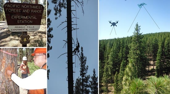
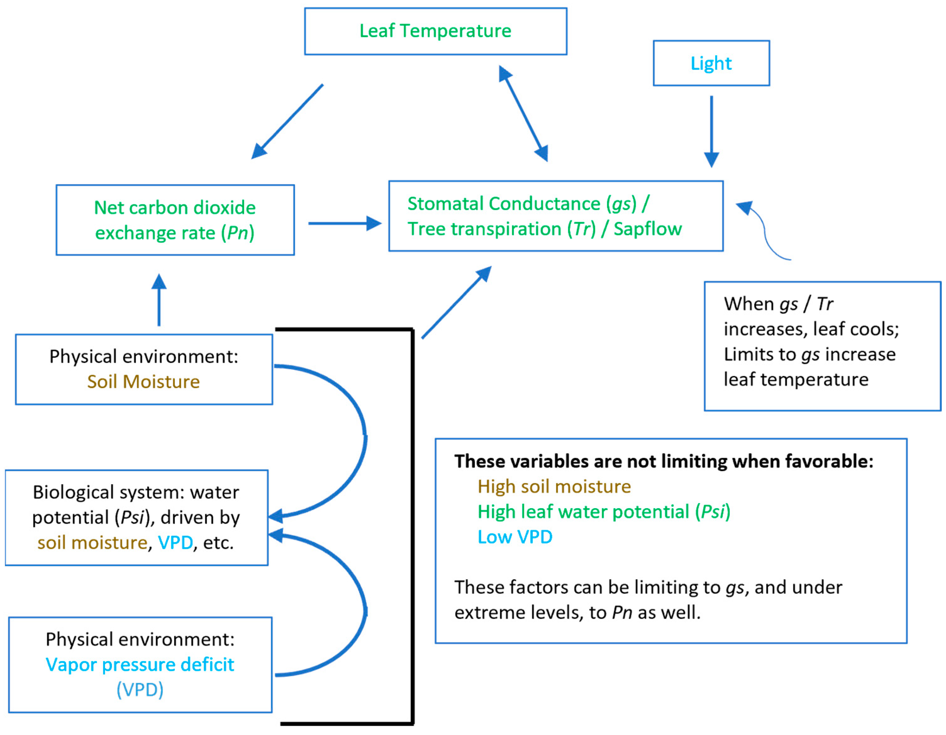
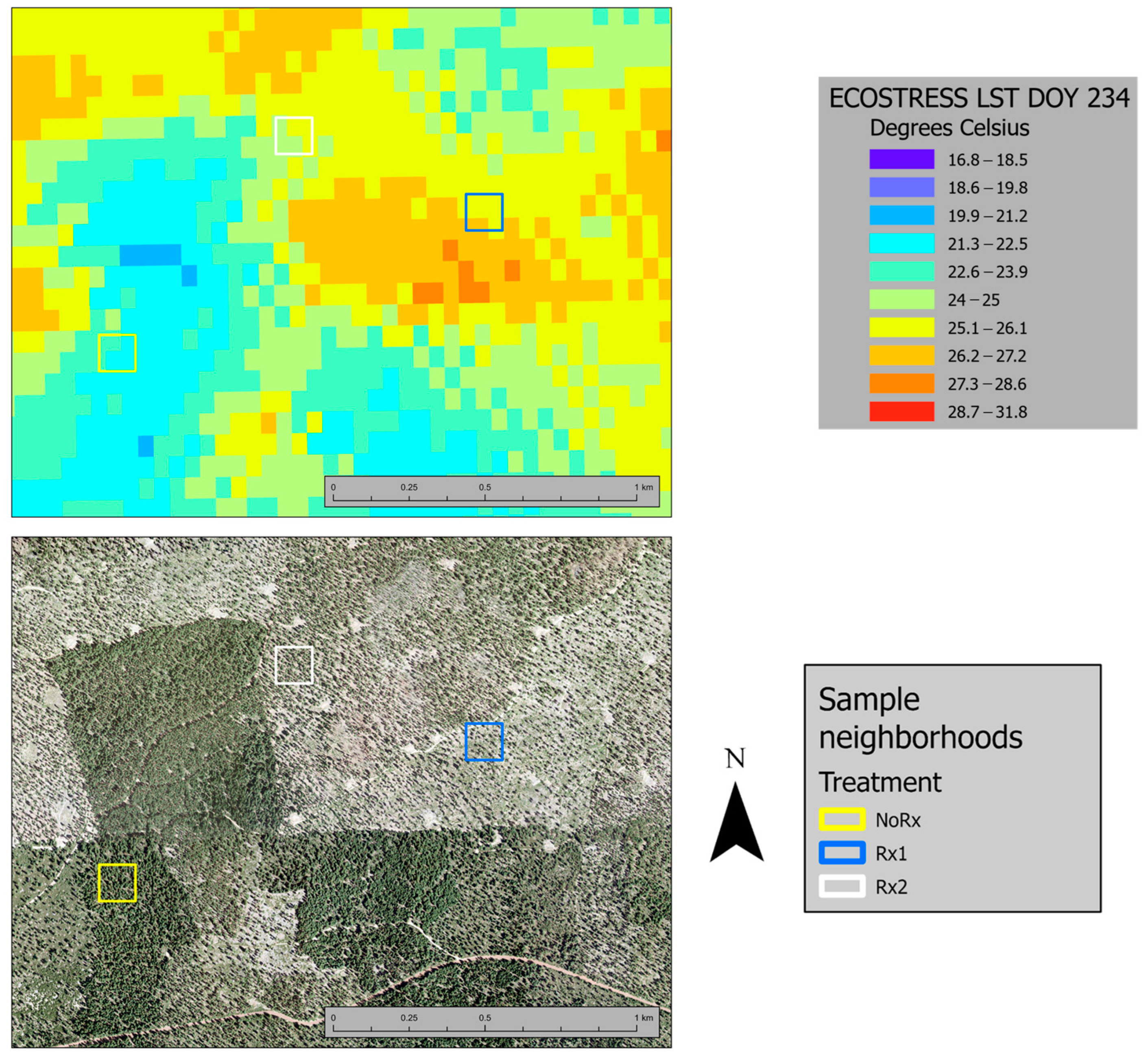
2.1. Site Location

Mature PP trees were monitored in the Pringle Falls Experimental Forest (43.78°N, −121.68°W/1584 m in elevation) managed by the Pacific Northwest Research Station of the USDA Forest Service. Soil characteristics are dominated by a dactite pumice deposition from an eruption of Mt. Mazama (now Crater Lake) 6600 years ago. Annual precipitation averaged 102 cm, with most precipitation falling in the fall and winter. We investigated stands within mature ponderosa pine stands representing three levels of density (TPH, trees per hectare) and basal area (BA, m2/ha). The selected density conditions resulted from two intensities of thinning—a light thin (Rx2), a heavy thin (Rx1), and an unthinned area representative of the untreated condition (NoRx). These treatments were conducted under the Lookout Mountain Thinning and Fuels Reduction Study (LOMS) [9]. The LOMS is a long-term experiment (proposed 50 years) to test the effectiveness of thinning treatments in achieving stand health and fuel reduction objectives.

2.2. Stand Characteristics

Within the LOMS, forest stands have similar elevation, aspect, plant association, soils, and topography. The plant association of the stands studied is CW-S1-15 (mixed conifer/snowbrush/sedge) [45]. The association consists of PP, a seral dominant species, with smaller amounts of grand fir (Abies grandis [Douglas ex D. Don] Lindl.), white fir (Abies concolor [Gord. & Glendl.] Lindl. ex. Hildebr.), and lodgepole pine (Pinus contorta Douglas ex Loudon), listed in descending order of abundance. Shrub species in the understory are dominated by greenleaf manzanita (Arctostaphylus patula ex. Greene) and snowbrush (Ceanothus velutinus Douglas ex Hook) [9,45].
We selected groups of dominant trees in each treatment type that were free of crown or bole defects and were also within ca. 60 m of each other, which was a prerequisite for connecting the sapflow equipment to a single data logger. These study sites, or ‘neighborhoods’, are shown in Figure 2. Pre- and post-treatment stand and tree metrics are given in Table 1. Ocular estimates of PP canopy cover are Rx1—15–20%, Rx2—40–60%, and NoRx—75–80%. The objective of the LOMS was to lower the risk of stand replacing wildfire risk by reducing understory fuel loads and stand density. The silvicultural prescriptions specified a preference for retention of fire and drought-resistant PP (e.g., large, mature trees) and for removal of lodgepole pine, grand fir, and white fir [9].

2.3. Whole Tree and Crown Morphological Attributes

For each intensively measured tree, we recorded GPS location, bole diameter at 1.37 m above ground level, height (clinometer), and percent live crown. An increment borer was used to extract a core sample. We recorded the tree’s age, length of sapwood, and total length of the core; the conducting sapwood area was calculated to relativize transpiration rates.
In addition to stand density, we assessed individual tree-to-tree competition (competitive zone density, CZD [47]). The reported CZD is the average of the diameter divided by distance to the closest neighboring tree >10 cm in four pie-shaped aspects around the tree out to a maximum distance of 20 m; if there were no neighbors in a pie, the value recorded was 0.
Tree crown attributes related to vigor and drought stress in PP [14] and a related species, Jeffrey pine [18], have been previously described and are presented in Appendix A. On each tree, 3 secondary branches and 3–4 branchlets back from the apex of primary branches in the upper third of the sunlit crown were used for morphological measures. Tree climbers accessed the crown of these mature trees to remove and drop sample branches for measurement. Among nearly 45 tree and crown attributes, the following morphological attributes have been correlated to tree bole production: needle and branchlet elongation growth (NL and BRN, 1 mm), branchlet diameter growth (BRIDIA, 0.1 mm), the level of needle chlorosis (CHL, ocular estimate), and disease incidence (DISEASE), a sum of the frequency of abiotic and biotic vectors [48,49]. Among these, needle elongation growth of current year (NL1), branch elongation growth of prior year (BRN2), and chlorosis (oxidative stress) are indicative of the level of drought stress in the current year. These metrics are presented as relative to the longest needle (NL1%) and branchlet (BRN1%) length on that sampled branchlet. Morphological attributes were collected the week of 13 August 2019 from 22 trees in the three neighborhoods: 8 in Rx1, 8 in Rx2, and 6 in NoRx.
The coordinates of each tree were recorded with a Garmin 60 CSX GPS (Garmin, Inc. Olathe, KS, USA) receiver; if the position error was greater than 10 m, we moved to a more favorable position and recorded the distance and azimuth to the tree from the new position.

2.4. Tree-Level Transpiration

Tree transpiration was calculated from sapwood area and sapflow rate measured with thermal dissipation probes (TDP-30, Dynamax, Inc., Houston, TX, USA) per [50] interfaced with a data logger (CR1000, Campbell Scientific, Inc., Logan, UT, USA) via 15, 25 or 30 m cables. Power was supplied by a deep cycle marine 12-volt battery supported by a 0.7 m × 1 m solar panel. A single TDP-30 probe pair was installed on the north aspect of each sample tree into the sapwood following removal of the bark within ~5 mm of the cambium. Each probe pair was then encased in Styrofoam for thermal insulation and covered with a reflective, waterproof shade. The lower probe delivered heat and the upper probe detected heat transfer, with the heat transfer a function of rate of sap flow (cm/hr., Etrans). Sapflow velocity was normalized by estimated sapwood area using methods described in [49] and recorded hourly. Sapflow data were collected on a total of 20 trees: 7 in Rx1, 6 in Rx2, and 7 in NoRx.

2.5. On-Site Temperature, Vapor Pressure Deficit, and Humidity

Air temperatures were extracted from existing data bases associated with the LOMS [9] and are given here for the purpose of comparing the weather conditions during the two-day data collection. Temperatures reported here were collected at each stand with an iButton temperature logger (DS-1922L Thermochron, Maxim Integrated Products, San Jose, CA, USA) mounted at 1.5 m above ground on fiberglass rods and sheltered from direct sunlight with inverted, feathered, plastic cup shades. Temperatures (°C) were recorded hourly for DOY 232 and 234. Averages for time of day approximating the UAV and ECOSTRESS collect times are presented in Table 2.
Vapor pressure deficit (VPD) and relative humidity (RH) are important parameters driving transpiration (see Figure 1). To estimate VPD and RH, we downloaded data from the Parameter-Elevation Regressions on Independent Slopes Model (PRISM) for DOY 232 and 234 [51] and these are estimated for 1.5 m above ground. These data are presented in Table 3.
To ascertain the drought status for the study area, we used data from the USDA Forest Service Drought Summary Tool (https://toolkit.climate.gov/tool/usfs-climate-gallery-drought-summary-tool-storymap, accessed on 13 October 2023) These data indicate that the study area experienced moderate drought in 2019, mild drought in 2017 and 2018, and a water surplus for the years 2010–2016.

2.6. Remote Sensing Data Collection

Unless otherwise noted, all GIS functions were performed in ArcGIS Pro v 3.1.2 software [52]. We employed two aerial vehicles (UAVs) to conduct a near-surface [crown] data collection campaign over the neighborhoods on 22 and 24 August 2019 (DOY 232, 234). These vehicles were manufactured by Dji (SZ DJI Technology Co., Ltd., Shenzhen, China). The Dji Phantom 4 Pro was mounted with the FLIR VUE Pro R 640 thermal camera (FLIR, Teledyne FLIR LLC., Wilsonville, OR, USA) and the Dji Inspire was mounted with the Micasense RedEdge MX multispectral sensor (MS, AgEagle Aerial Systems, Inc., Wichita, KS, USA).
The FLIR instrument is primarily used in detecting high-energy targets such as wildland fire hotspots and has a documented accuracy of ±5 °C or 5% of the returned value. A similar FLIR instrument was tested and uncalibrated FLIR temperatures were within 1.2–1.4 °C of leaf thermocouple temperature measurements [41] They concluded that for conifer thermography applications in the range of 10–25 °C, correction was unnecessary and that factory default settings were adequate. Spectral bandwidth for the FLIR is 7500–13,500 nm. Band specifications for the MS are listed in Table 4 below.
A north to south ‘lawnmower’ flight pattern was used over each neighborhood, starting west and finishing east. The pattern was pre-loaded into the UAV and flight control was conducted with a GPS/GLONASS satellite positioning system that is rated to be accurate to within ±0.5 m vertically and ±1.5 m horizontally. Flying height was determined with the aid of a digital terrain model and was approximately 90 m above ground level and ~70 m above tree crowns. For the Dji Phantom carrying the FLIR camera, nominal endlap and sidelap were 90% and 75%, respectively. For the Diji Inspire mounted with the Micasense instrument, nominal endlap was 85% and nominal sidelap was 80%. Each 2 ha plot took ~4–5 min to image, largely depending on the flight distance to and from a landing area clear of obstacles.
UAV flights were conducted 20 and 22 August 2019 (Day of Year, [DOY] 232 and 234). The Rx2 and NoRx sites were imaged with both instruments on DOY 232. DOY 233 was a no-fly day due to inclement weather. On DOY 234, we flew the NoRx neighborhood. For each neighborhood, we conducted three flights per day, targeting before noon (am), noon, and afternoon (pm). Our intent was to capture diurnal patterns in MS or FLIR to relate to the hourly Etrans data. Flight times for each of the neighborhoods are presented in Table 5. The MS imagery was georeferenced using Pix4Dmapper software version 4.6.3 [53] which uses Structure from Motion algorithms to calibrate and align the overlapping images. Radiometric calibration was performed using camera parameters and solar irradiance; we did not use reference panel data. We estimate that this had a negligible effect on the multispectral data collected with the MicaSense instrument as the collects all occurred in the same day under the same lighting conditions. Since the images did not contain location information, ground control points (GCPs) were located on Oregon Statewide Imagery Program 2018 natural color orthomosaics and used to georeference and orthorectify the multispectral images. A separate 16-bit image was created for each MS band.
The FLIR images were processed in FLIR Thermal Studio v 1.9.10 software [54]. Thermal parameters (emissivity, reflected temperature, atmospheric temperature, relative humidity, reference temperature) were adjusted based on PRISM data, at-sensor temperature at the time of image collect, and an emissivity of tree species value (0.95). These corrected radiometric images were then opened in Pix4Dmapper v 4.6.3 software [53], where they were converted to 32-bit unsigned surface temperature grids. At the nominal flying height of 90 m, images from the FLIR instrument were 100 cm in resolution following post processing. FLIR and MS orthomosaics of each neighborhood were created in Agisoft Metashape software version 2.1 2020 [55].
A total of 23 trees were imaged with the Micasense sensor; Etrans data were available 2 for 13 of these. All 23 trees were imaged with the FLIR instrument.
Multispectral (MS) data were processed into indices which are mathematical combinations of 2 or more bands (Table 6). We also selected the RE, R, B, and NIR bands for analysis. This suite of bands and indices was chosen based on their utility in detecting stress and phenological status in conifers [18,19,56]. The final MS outputs were 16-bit unsigned 6 cm resolution img files, one file for each band/index.
Using the physics-based Temperature and Emissivity algorithm [52], ECOSTRESS TIR data were used to generate georeferenced land surface temperature images (ECO2LSTE v001). These images are available via the USGS Earth Explorer web tool. At our study site location, the ECOSTRESS pixel was 38 m height (latitude) × 69 m wide (longitude). We downloaded the ECO2LSTE v001 images that were collected on our UAV flight days (DOY 232 and 234). These collection times are listed in Table 5. ECOSTRESS temperatures for each tree were extracted from the downloaded grids using GIS software (ESRI 2023). ECOSTRESS land surface temperature pixel values (Tes) were assigned to the 29 tree crowns with Etrans data. There were six unique ECOSTRESS pixels with Etrans trees on DOY 232 and 9 on DOY 234; this discrepancy is due to the inconsistent orbital characteristics of the ISS, which results in slight changes in the ECOSTRESS pixel configuration between acquisitions. The number of Etrans trees in an ECOSTRESS pixel ranged from one to six. The ECOSTRESS LST (Land Surface Temperature) raster layer for DOY 232 is displayed in Figure 3.

2.7. Data Compilation and Analysis

We used the GPS coordinates of each of the intensively studied trees with the MS and FLIR orthomosaics to aid in locating the tree crowns on the FLIR and MS image tiles. Image tiles were selected that best displayed the sunlight portion of the tree crown. The sunlit portion of each tree crown was digitized, and the resulting polygon used to extract statistics (mean, standard deviation) from the image tile. When digitizing the polygons, we always included the top of the tree and excluded any areas with dead branches and large shadow areas. This process was conducted for both the MS and FLIR image data. The ESRI Zonal Statistics tool [52] was used to create a table of MS and FLIR statistics for each digitized tree crown polygon.
When comparing the morphological attributes, which do not vary by time of day, we used the pm Td and Etrans values. For MS analysis, we used the noon and pm Td and Etrans values because of the xeromorphic characteristics of conifer leaves; any spectral response would be attenuated until noon when the light intensity on the crowns is greatest [59,60]. When comparing Td to Tes, we used the Td value that was the closest to the time of the Tes collect, so in this case we had 20 data points. In the Tes-Etrans analysis, we used the Tes values for both DOY 232 and 234, a total of 40 data points.
All data (Etrans, Td, Tes, MS band and index values, morphological attributes) for each tree crown were compiled into Microsoft Excel [61] spreadsheet tables. We reconciled the date and time of the data points such that they matched temporally. Etrans was interpolated between hourly measures to match that of the UAV and ECOSTRESS acquisitions. We adjusted the Etrans time by adding 1 h to compensate for the lag between Etrans measured at the bole and when that sap reaches the terminal branch foliage where it will affect crown temperature and spectral reflectance [62]. Similarly, FLIR measurements were matched to the once-a-day time of satellite acquisition. This table was the source for the statistical tests and summaries described below, which were carried out using RStudio v 2022.12.1 Build 402 [63] and R v 4.2.1 [64].
We tested our data to see if the assumption of a normal distribution was met using the Shapiro–Wilk normality test. All statistical tests were evaluated at the 95% level. To test for differences in the means of Td, Tes, and Etrans, we conducted one-way analysis of variance ANOVA tests followed by Tukey Multiple Comparison of means tests. Correlation matrices to examine the relationships between Etrans, MS, Td, Tes, and the morphological attributes were calculated using the cor_pmat function in R [64]. Similarly, linear regression models were built with the lm function to visualize the Td and Tes correspondence to Etrans and the CZD-Td relationship. Stepwise multiple regression models were created to determine significant predictors of Td and Etrans.

3. Results

An average of 124 image tiles were collected over each neighborhood for each of the instruments (FLIR and MicaSense) and corresponding platforms; examples of the image tiles are displayed in Figure 4.

3.1. Tree Morphological Attributes and Transpiration by Treatment

The number of needle ages (#WHL) and branch diameter (BRDIA2) did not differ among trees sampled in the three density stand levels (Table 7). Needle and branchlet elongation, relative to the longest branchlet elongation observed, were lowest in Rx1, the heavily thinned stand, and needle lengths of trees in both thinning treatments were lower than the unmanaged stand. Oxidative stress (i.e., chlorosis) was much greater in current year needles (CHL1) than in prior year needles (CHL2) on all sites. In Rx1, chlorosis was 1.25 times greater in current vs. prior year needles; in Rx2, chlorosis was 1.52 times greater, and in NoRx, chlorosis was 3.09 times greater than in the prior year. Chlorosis in 4-year-old needles was greatest in Rx1 (~30%), and chlorosis in Rx2 and NoRx was lower and similar (~20%). The attributes summarized in Table 7 were used in the Etrans and Td stepwise regression models.
Transpiration of instrumented trees followed a parabolic curve, in sync with diurnal light levels (Figure 5). Note the significantly lower transpiration rate during a cloudy day of lower temperature (DOY 233) not used in the present analysis.
Mean Etrans values were higher in Rx1 than NoRx, evidence that trees in the heavily thinned neighborhood had greater conductance than in the unthinned site and, by inference, were more photosynthetically active. No difference between Rx1 and Rx2 indicates that this level of thinning confers no improvement in Etrans, while the marginally insignificant (p = 0.076) difference between Rx2 and NoRx is some evidence that the light thinning offers no Etrans advantage over no thinning. The Etrans trend across neighborhoods was the inverse of UAV FLIR temperature (Td); the highest Etrans neighborhood was Rx1, followed by Rx2 and NoRx. The attributes summarized in Table 8 were used in the Etrans and Td stepwise regression models.

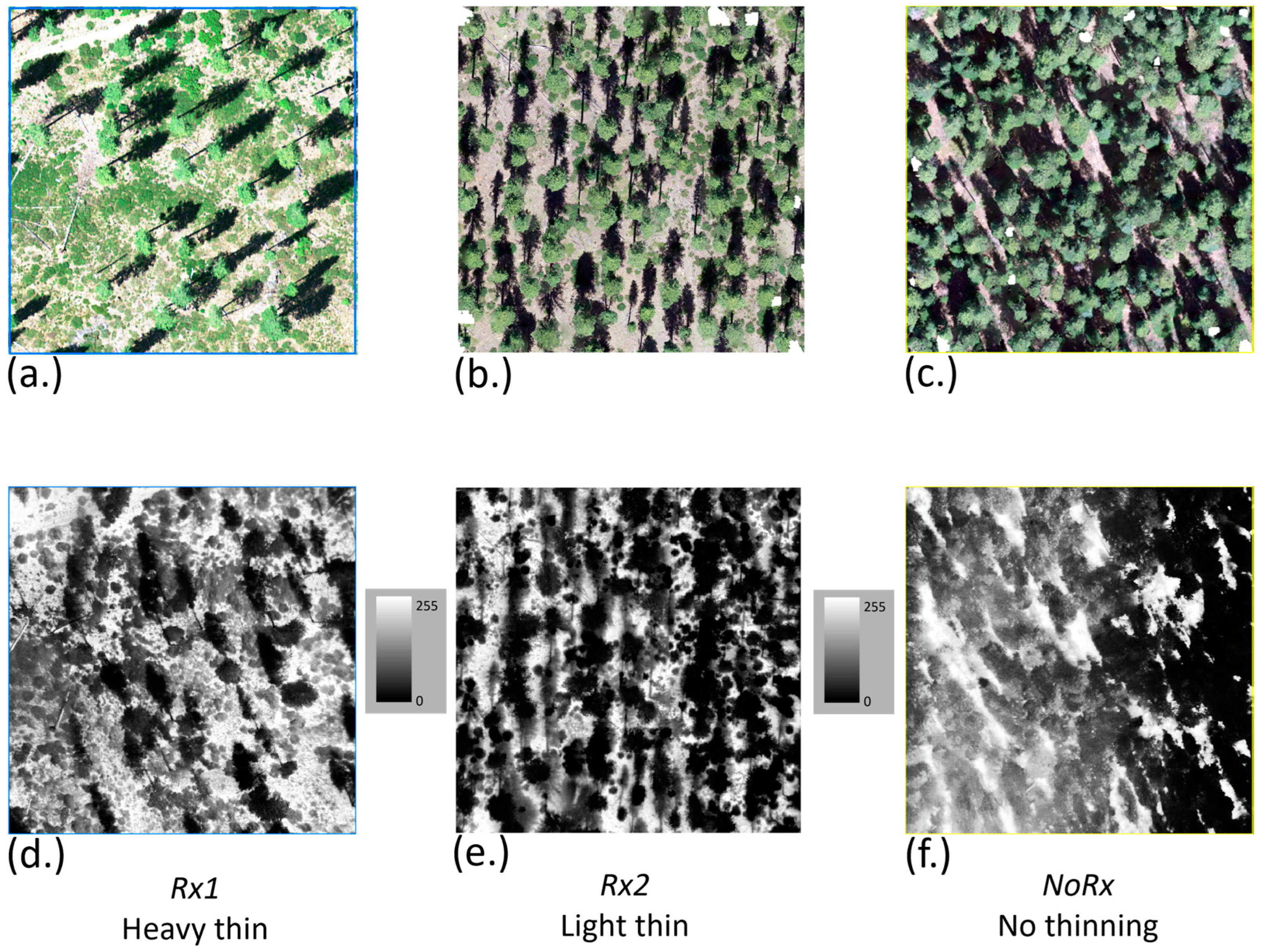
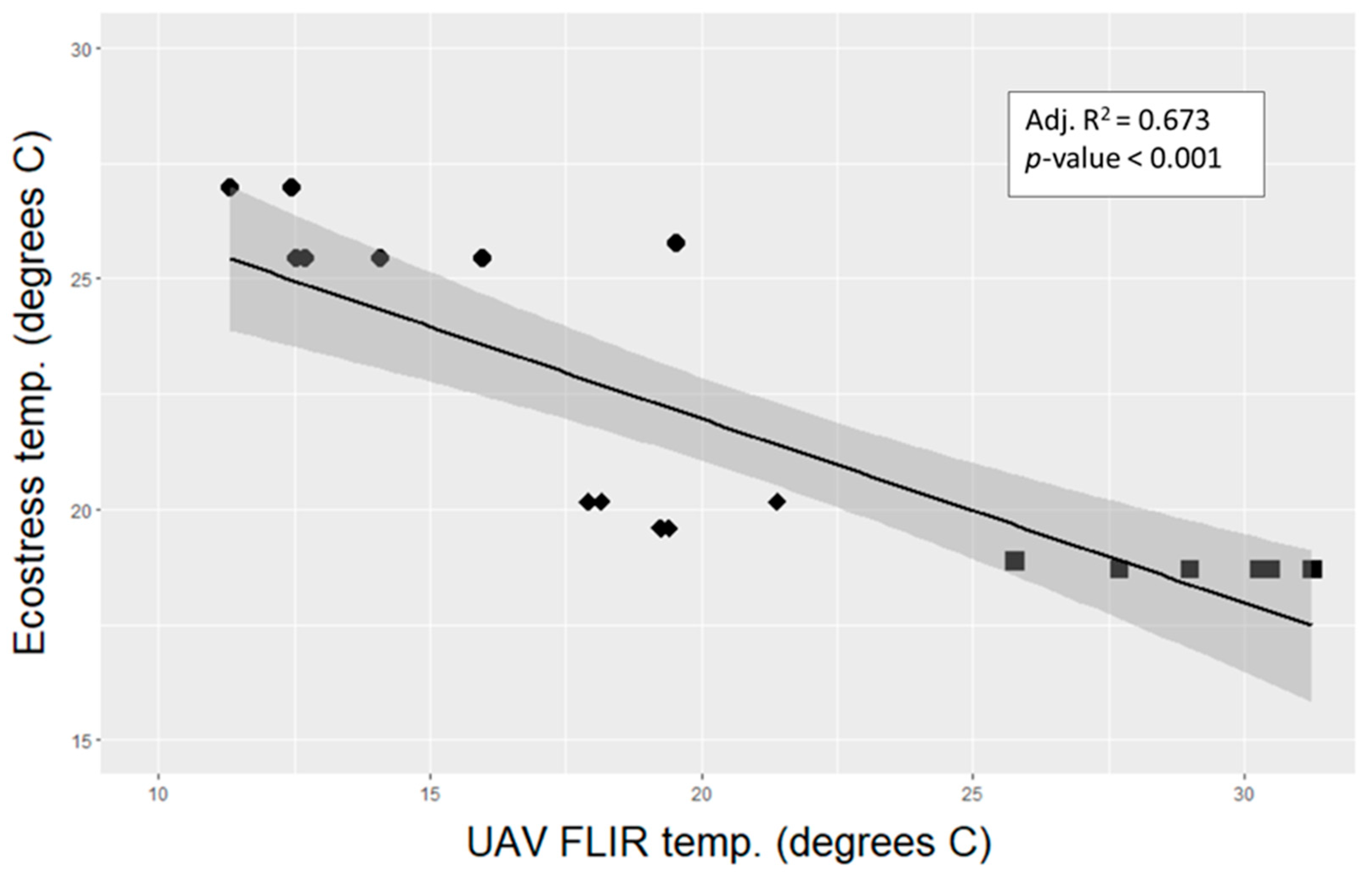
3.2. Remote Detection of Crown Temperature

All temperature variables met the assumption of normality (Shapiro–Wilk). Mean Td differed across all neighborhoods. However, the cool and wet weather on DOY 234 (Table 2 and Table 3) somewhat invalidates any comparison with Rx1. In NoRx, lower windspeeds in a denser canopy coupled with greater crown temperatures were likely to cause higher foliar transpiration (saturating water within the needle, higher temperatures inside and outside of the needles, but greater air evaporative demand) and greater tree drought stress. This is supported by the higher oxidative stress and crown temperatures (Td) observed (Table 7 and Table 9) in NoRx.
The temperature trends were reversed for Tes and Td; the highest Tes neighborhood was Rx1, followed by Rx2 and NoRx, (Table 10), while for Td, NoRx was the warmest, followed by Rx2 and Rx1. Note the different spatial scales of the two metrics: Tes is land surface temperature across a 38 m × 69 m area and Td is averaged over the upper one-third of selected tree crown, with shadows and branch surfaces excluded. The scatterplot of Td vs. Tes captures the negative correlation between the two crown temperature measures and distinct grouping of the Rx types (Figure 6).

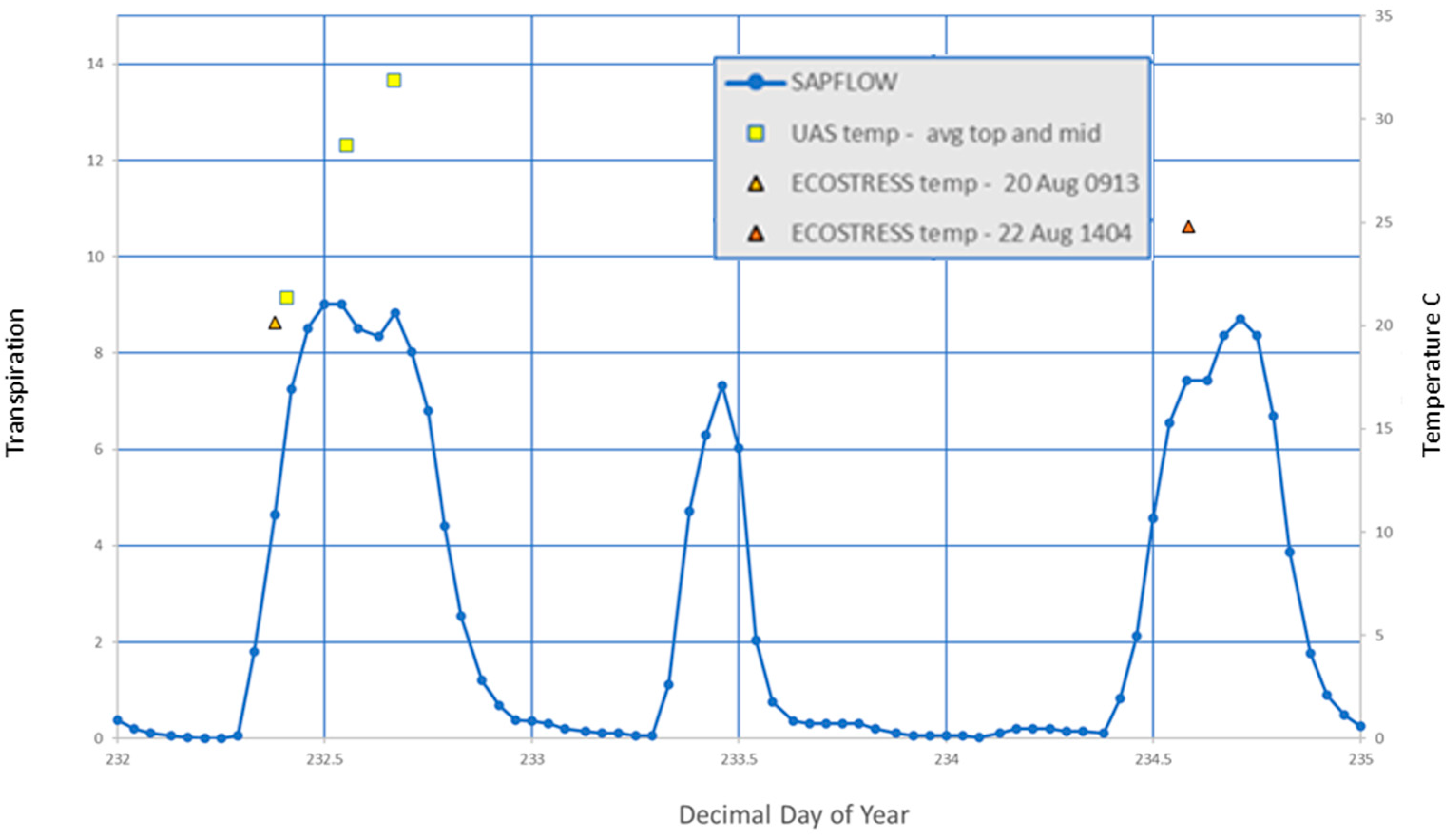
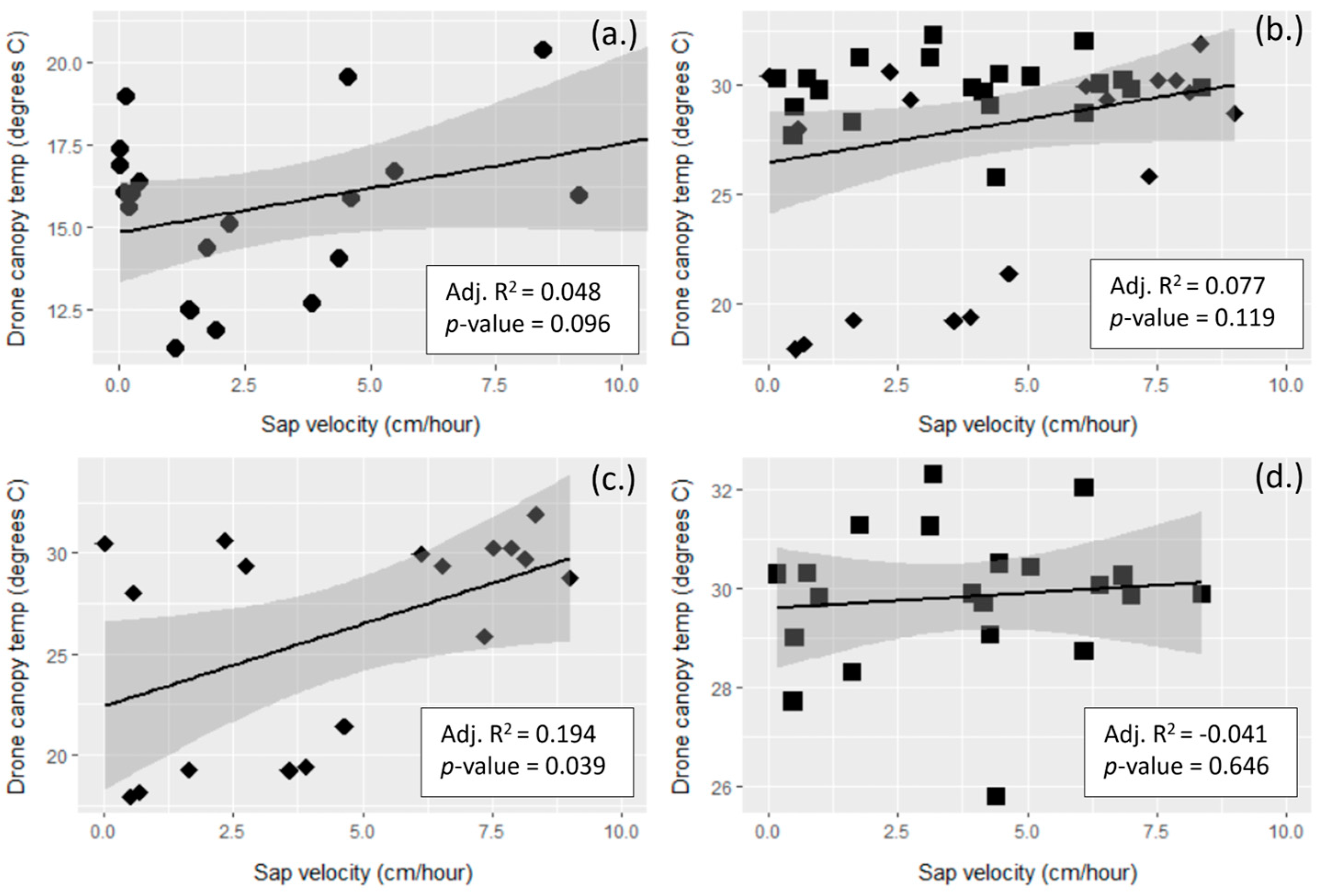
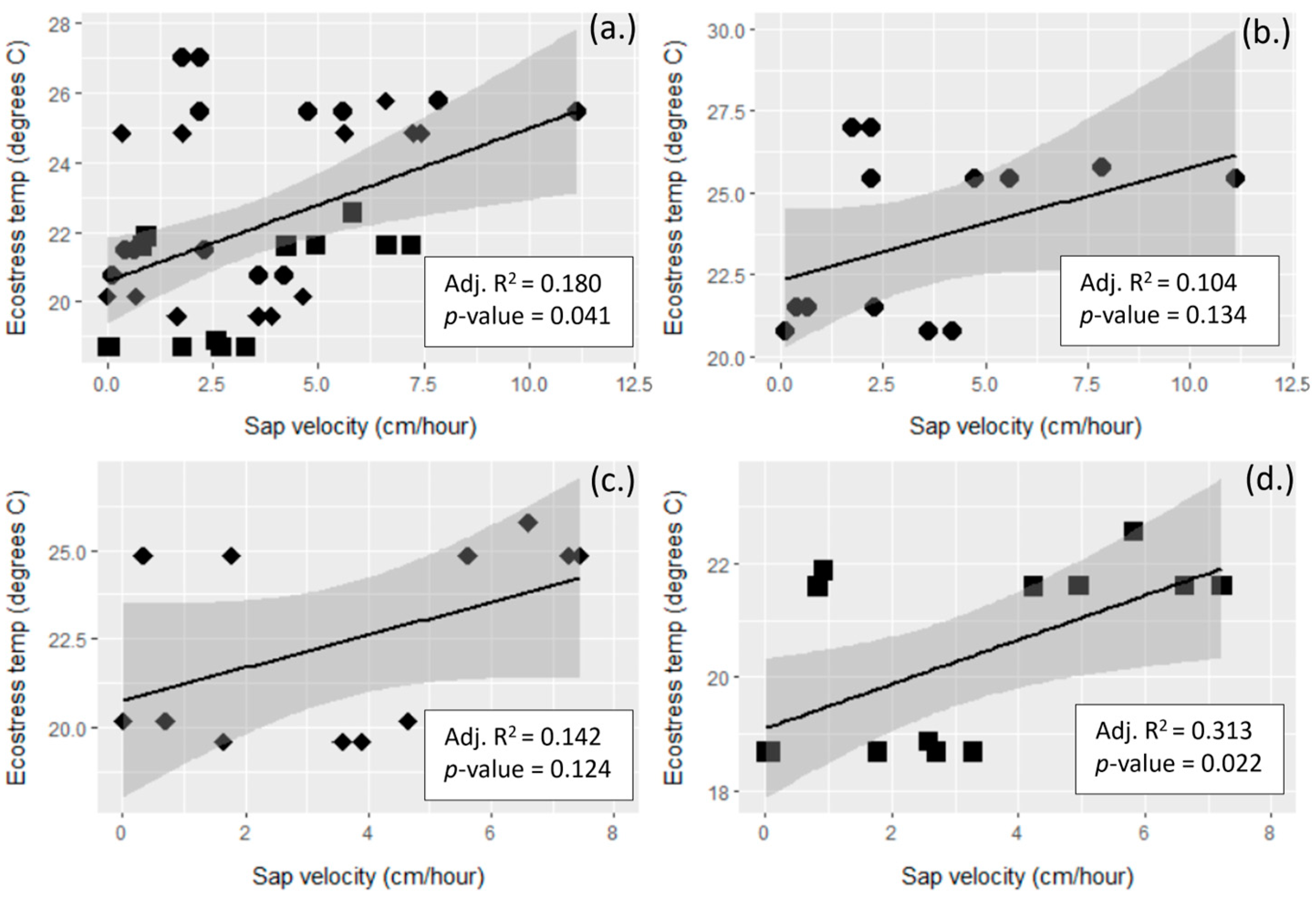
3.3. Remotely Sensed Temperature vs. Tree Transpiration

Td crown temperatures had a weak, positive correlation to sapflow for Rx1, Rx2, and all three neighborhoods combined (Figure 7). Only Rx2 was statistically significant.
ECOSTRESS LST temperatures for both DOY 232 and 234 showed a similar pattern, with the higher density Rx2 and NoRx neighborhoods having the strongest correlation with Etrans (Figure 8).

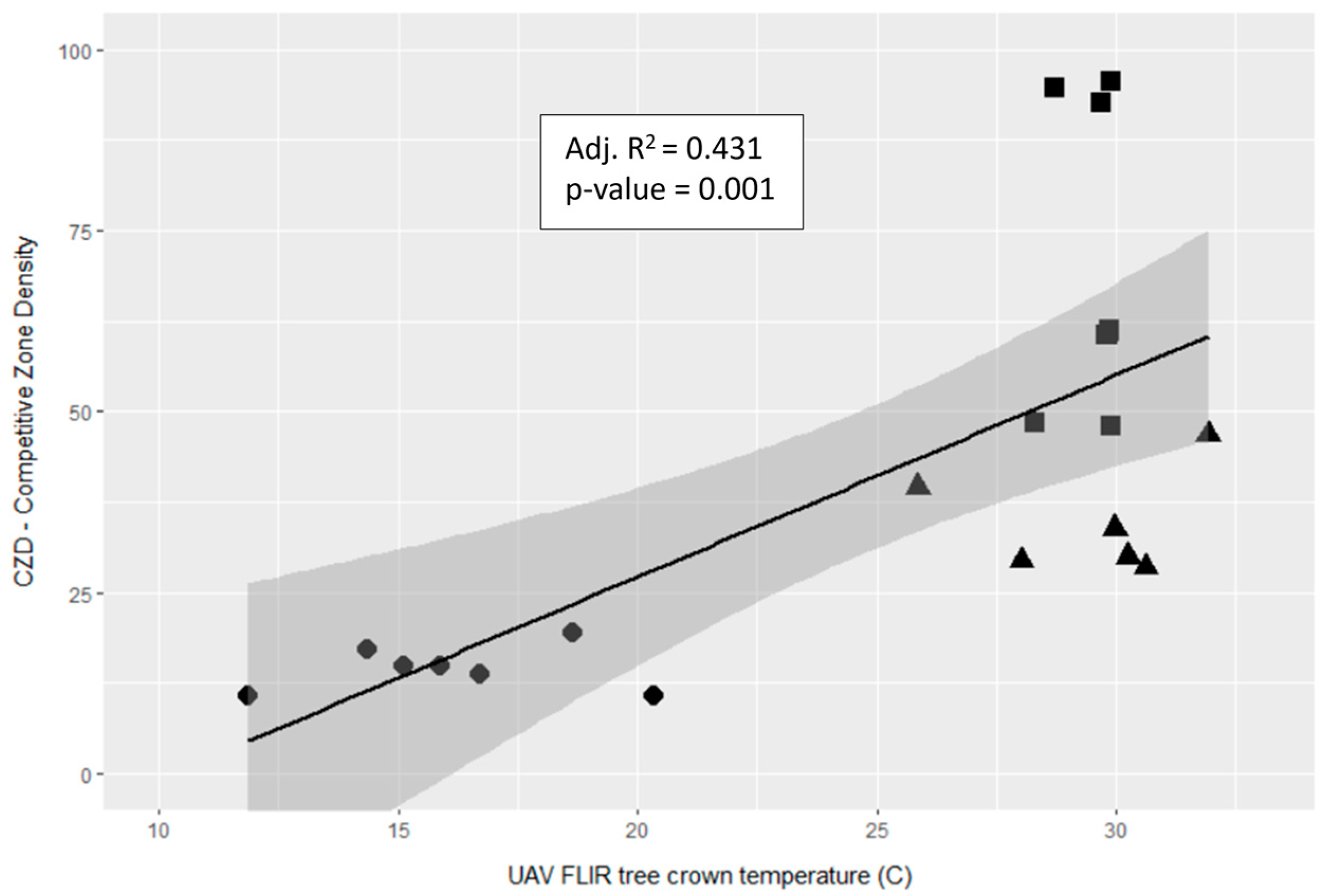
3.4. Contributing Predictors of UAV FLIR Crown Temperature (Td)

We explored whether Etrans, Rx (ordinal), or tree to tree competition (CZD) were predictive of crown temperature (Td) using stepwise multiple linear regression (Table 11).
The model had a high degree of correlation (Adj. R2 = 0.783) and identified significant differences between Rx1 and Rx2, and Rx1 and NoRx. As a contributing predictor, Etrans was significant (p = 0.039), but tree-to-tree competition (CZD) was not. Predicting drone-detected crown temperature from only Etrans and CZD was not as effective overall (Adj. R2 0.528, p = 1.94 × 10⁻¹⁰ AIC = 192.83), although a significant correlation between CZD and Td was found when no other attribute was co-analyzed (Figure 9). In this figure, trees in the different neighborhoods are clustered together with the Rx2 and NoRx trees in the same 5–7 °C range, but the Rx2 trees have a significantly lower mean CZD (30.1) than the NoRx trees (71.6).
The CCI and NDVI spectral indices and the B and R bands have significant correlation to UAV FLIR tree crown temperature (Td) (Figure 10, Table 12). To reduce the effects of collinearity, we removed R and Re from the stepwise regression model as they were highly correlated (≥Adj. R2 0.80) with B and NDVI (R) and NIR (Re).
For the trees in the NoRx and Rx2 neighborhoods, CCI was the strongest predictor of crown temperature (Td), followed closely by NDRE and NIR.

3.5. Contributing Predictors of Tree Level Transpiration (Etrans)

When combined in the same stepwise linear model, both crown temperature measurements (Tes and Td) were significant predictors of Etrans, along with stand type (Table 13). Within the model, Tes was a stronger predictor than the average per-pixel Td values. Similar to the Td model (Table 11), CZD was not significant and the difference between Rx1 and NoRx was significant in the Etrans model (Table 13).

4. Discussion

In this study, we tested for correlations among remotely sensed metrics (thermal and multi-spectral) from different platforms (UAV and space-borne) and tree crown-based morphology attributes associated with tree drought stress and sapflow measures of transpiration. Our objective was to evaluate these remote sensing and field methods for their potential effectiveness in evaluating the water balance of different forest treatments in a drought year.
The reverse pattern of Rx temperatures from ECOSTRESS (Tes) and the UAV FLIR sensor (Td) is intuitive when mixed pixels for the former and individual trees for the latter are considered. At a nominal resolution of 2600 m2 (38 m × 69 m), a large percentage of a Tes pixel is shrub/forb vegetation and bare ground in an Rx1 stand; these surfaces tend to be much warmer than the sparse cover of the overstory conifers.
The understory was dominated by Arctostaphylos patula, which at the time of season (August), was likely to have been water limited, resulting in higher foliar surface temperatures. At the other end of spectrum, an ECOSTRESS pixel in an NoRx stand is dominated by tree crowns, and the ground cover is shaded and minimized. This is the mixed pixel effect. For this reason, the NoRx Tes are the lowest of the three neighborhoods. However, when we look at the individual tree crown temperatures (Td), the mean Td for trees in NoRx is significantly higher than Rx2 (comparison to Rx1 is not possible due to confounding weather conditions), suggesting that NoRx trees are under greater drought stress than Rx2. Density reduction treatments such as those conducted as a part of the LOMS have been shown to reduce tree drought stress and related mortality [42,65]. Trees in the high-density NoRx neighborhood (SDI = 282) are likely under greater water deficit due to higher levels of tree-to-tree competition (CZD) and reflect that with higher crown temperatures than the thinned neighborhoods. This is the pattern we observed with the Rx2 and NoRx neighborhoods. Higher crown temperatures in NoRx could also have been influenced by high tree density with lower wind speeds at the level of the upper crown and re-radiation of higher temperatures from tree to tree at that height.
ECOSTRESS is effective at tracking conifer canopy temperature seasonally [17], evapotranspiration in post-fire Mediterranean biomes [66], and drought stress in agricultural crops [67], but applications in conifer forests are few. The higher Td crown temperatures we observed for individual trees in NoRx are likely cancelled by the cooling effect of shadows and dense canopy architecture at the scale of an ECOSTRESS pixel. Similarly, the cooler Td in Rx1 was not observed in Tes due to the high temperature of shrubs and bare ground. ECOSTRESS is a land cover assessment tool that could be used to assess the relative drought stress of high canopy cover stands, but it is too coarse in resolution for tree-level assessments. Tes and Td are different tools for different objectives, and different conclusions on tree transpiration/water balance (and tree drought stress) would be drawn if not used in tandem.
Although the cooling effect of gas exchange at the leaf level on leaf temperature is well documented [68,69,70], neither FLIR (Figure 7) nor ECOSTRESS (Figure 8) thermal imagery in our data showed greater crown temperatures with lower tree transpiration. Our data showed only a weak, mostly non-significant, positive correlation between Etrans and crown temperature, suggesting that stomata remained open as air temperature increased; this increase led to a modest rise in canopy surface temperature without a decrease in Etrans. Leaf and canopy temperatures are a product of many environmental and structural traits in addition to transpiration [36]. The Etrans-Td relationship we observed is likely a product of canopy and leaf architecture, the leaf to air temperature gradient, and the canopy microclimate [26,69].
Our growth data were inconclusive in supporting greater tree drought stress with increasing tree density; needle retention and elongation, branch elongation, and diameter did not show a definitive trend [39,54]. Lower elongation growth suggests less water availability and greater tree drought stress in the same year of growth. We expected that trees on the thinned site would be less drought stressed, but we found that they generally had lower elongation growth, perhaps due to greater crown evaporation due to increased wind flow through a heavily thinned stand. Also, there may have been significant competition for water between the pines and shrub cover; in the Great Basin, shrubs outcompeted pine for water [71]. Branchlet diameter (BRDIA) is correlated with basal area increment and is also indicative of reduced carbon acquisition and allocation to wood production in that year and the following year [14,60]; we observed no difference in BRDIA among the treatments. Increased needle chlorosis from 2018 to 2019 reflected a shift from mild to moderate drought stress in the year of this study and greater oxidative stress in NoRx followed by Rx2 and Rx1; a similar pattern is seen in CZD. Chlorophyll repair from oxidative stress requires nutrient uptake from the soil (water, magnesium, nitrogen, in order of priority), and repair is prioritized from current to older needle ages [47].
Trees under low drought stress are unlikely to exhibit the expected negative correlation between crown temperature (Td) and transpiration (Etrans). Under low water deficits, canopy temperature is driven mostly by environmental conditions (weather, canopy structure) rather than transpiration and stomatal conductance. This is likely the situation with our study trees. Based on crown and tree attributes, tree vigor was greater in this study than PP at a site experiencing less precipitation and more evaporative demand [14]. We report 1.56× more needles retained (#WHL), 1.65× greater branch diameters (BRDIA), 1.70× branch length (BRN%), and 1.43x more chlorosis in the 4th year (CHL4) for mature PP at PFEF vs. their site in south central Oregon. Our study area was in moderate drought in 2019, but in the previous nine years, two were mild drought while seven were water surplus years.
Increased stand density in mixed conifer forest types due to fire suppression is a well-known cause of increased drought stress [11], although there is evidence that PP in lower densities is less resistant to drought stress than in higher density conditions [72]. We found that density at the tree-to-tree level (CZD) was not a significant predictor of either transpiration (Etrans) or crown temperature (Td); however, stand (Rx) effects were. CZD has an inconsistent association with Etrans at values of up to 40 m2/ha; above this threshold, there is a steep decline in Etrans [47]. Except for NoRx, the mean CZD of the study neighborhoods was below this threshold, which may explain the non-significance of CZD. Stand density is a stronger and significant predictor of crown temperature and transpiration; from a manager’s perspective, this is helpful as knowledge of the treatment alone (thinning level) may be used to improve tree vigor rather than labor-intensive measures of neighboring tree competitive pressure such as CZD.
Although availability of thermal imagery is improving, challenges regarding spatial and temporal resolution remain. As described above, long-wave radiation in the thermal infrared part of the electromagnetic spectrum is relatively low energy and large pixel sizes are necessary to capture the signal. TIR sensors are typically 1.5 to 2 times the pixel size of their VNIR counterparts. Despite new sources of thermal imagery such as UAV-mounted sensors like the one used here, VNIR options are more numerous and do not have the complex calibration correction steps often required with TIR sensors [36,40]. This prompted our investigation into the relationship between TIR tree crown temperatures and a variety of VNIR bands and indices from UAV platforms.
We found that CCI and NDVI indices had moderate positive correlations to Td, and B and NIR bands had moderate negative correlations. In our final model (Table 12), NDRE and CCI were significant. CCI is of particular interest as it has been promoted as an alternative to NDVI and other indices for tracking phenology based on its sensitivity to changing chlorophyll/carotenoid ratios seasonally in conifers [31,57] and in assessing carbon uptake [32,73]. To our knowledge, this is the first study to examine the use of CCI to assess drought stress and vigor in conifers, and its significance is an indication that further work is needed.
The red-edge band (Re) is a relative newcomer to the VNIR space and is spectrally located between R (625–700 nm) and NIR (800–1200 nm). NIR has long been used to track stressed vegetation [74] as color infrared film long preceded multispectral digital sensors. Red edge leverages the dramatic difference in chlorophyll reflectance between R and NIR. This part of the spectrum is highly sensitive to chlorophyll a and b [75], which are reduced when a plant is stressed [76]. It is effective in detecting stress in Scots Pine (Pinus sylvestris) in a nursery setting [58] and, when substituted for R in the NDVI formula (NDRE), in discriminating stress in a piñon-juniper stand earlier than NDVI [35].
Our work here shows that these VIs are reasonable proxies for the thermal signatures that characterize drought stress in conifers and are worthy of additional investigations.
Because of the decoupling of Td and Etrans in our data, we also investigated the relationship of Etrans with the multispectral bands and VIs. Re, NIR, and B showed moderate negative correlations, most likely driven by the increase in water and active chlorophyll associated with higher Etrans, which is not surprising for B but is somewhat puzzling for Re and NIR. By all accounts, the latter bands should have had a positive correlation with Etrans. Using our point in time approach, correlations between Etrans and VIs were elusive. However, foliar traits that were detected in the multispectral data were likely the product of tree transpiration and water status over days, weeks, and months and not simply at the time of spectral data capture.

5. Conclusions

This study is an investigation of the comparative use of disparate remote sensing technologies (UAV and ECOSTRESS) in assessing ponderosa pine drought stress in unmanaged and managed mixed conifer forest in central Oregon. Heavy thinning in PP resulted in trees exhibiting reduced drought stress (sustained transpiration) relative to those on unmanaged sites, but this was not observed in light thinning treatments. However, crowns on a lightly thinned site were cooler than those in an untreated control, indicating a reduction in drought stress.
UAV- and ECOSTRESS- detected tree crown temperature and transpiration measures were largely decoupled at this relatively mesic site, contrary to the commonly accepted paradigm that they are negatively correlated. Evidence suggests that our sample trees were under mild–moderate, but not extreme, drought stress, which could explain these observations.
Differences in ECOSTRESS pixel composition across the neighborhoods, e.g., a higher proportion of shrub, bare ground, and litter cover, likely contributed to the inverse relationship between UAV and ECOSTRESS temperatures. The best use of ECOSTRESS may be in thermal and transpiration comparisons between similar stand densities and at the landscape level, as the data are too coarse for tree-level stress detection. Visible and near-infrared bands and indices are inherently more accessible than airborne or near-surface thermography. The CCI, NDRE indices, and the NIR and B bands as gathered by UAVs show promise as possible proxies for crown temperature and drought stress. Image-based layers using these indices could be operationally developed that aid foresters in prescription marking and in selecting drought-resistant or -resilient seed source trees. Further research is warranted.

Author Contributions

Conceptualization, N.E.G. and C.S.-P.; methodology, N.E.G. and C.S.-P.; software, J.W., J.C. and C.S.-P.; validation, N.E.G., P.D.A. and C.S.-P.; formal analysis, N.E.G. and C.S.-P.; investigation, N.E.G.; resources, N.E.G.; data curation, N.E.G. and C.S.-P.; writing—original draft preparation, C.S.-P.; writing—review and editing, N.E.G., P.D.A. and C.S.-P.; visualization, N.E.G.; supervision, C.S.-P.; project administration, N.E.G.; funding acquisition, N.E.G. All authors have read and agreed to the published version of the manuscript.

Funding

Funding for this work was provided by the USDA Forest Service Western Wildlands Environmental Threat Assessment Center.

Data Availability Statement

Data available upon request, contact the corresponding author.

Acknowledgments

We thank Lisa Balduman for her help with field work and tree climbers Drew Peterson, Cristina Peterson, Phil Chi, and Chad Marks-Fife for their help in collecting branch samples. Also, we thank Jimmy Swingle and Eric Forsman for their help in setting up the tree climbing equipment and for retrieving a UAV from a tree.

Conflicts of Interest

Author Charlie Schrader-Patton, Jamieson Chaitman and Jeremy Webb were employed by the company RedCastle Resources Inc. The remaining authors declare that the research was conducted in the absence of any commercial or financial relationships that could be construed as a potential conflict of interest.

Appendix A

  • Branchlet diameter (BRDIA)—Diameter measured in mm (±0.01 mm) at the base of the previous year branchlet.
  • Branchlet elongation (BRN)—Measured length of the current year branchlet (±2.0 mm) (BRN1) or the previous year’s branchlet (BRN2). BRN1% is the percentage of the current year’s branchlet length relative to the maximum branchlet length of all annual branchlet length segments present on the branch.
  • Chlorosis (CHL)—Chlorosis level of needles expressed as a percent of healthy, green needles in the same age class by ocular estimation. Age class is indicated by integer, e.g., CHL2 is the chlorosis level for the previous year’s needle age class.
  • Insect and disease (DISEASE)—a sum of the frequency of abiotic and biotic vectors on sampled branches in each crown [14,48,49]. Abiotic vectors included needle tip dieback, whole needle dieback, and early needle senescence (in August instead of October), all likely driven by drought stress. Biotic vectors included presence or absence of pine needle weevil, phloem feeder, armored scale, black pineleaf scale, and needle blight (Latin authorities given in [14]).
  • Needle whorls (#WHL)—The number of needle ages retained on the branchlet. Ponderosa pine needles are in distinct groups on branchlets; these groups are established annually. See [14] for examples.
  • Needle elongation (NLN)—Measured length of the current year needle length (+2.0 mm) (NLN1). NLN2% is the percentage of the current year needle length relative to the maximum needle length retained on the branchlet.

References

  1. Allen, C.D.; Macalady, A.K.; Chenchouni, H.; Bachelet, D.; McDowell, N.; Vennetier, M.; Kitzberger, T.; Rigling, A.; Breshears, D.D.; Hogg, E.H.; et al. A Global Overview of Drought and Heat-Induced Tree Mortality Reveals Emerging Climate Change Risks for Forests. For. Ecol. Manag. 2010, 259, 660–684. [Google Scholar] [CrossRef]
  2. Fettig, C.J.; Mortenson, L.A.; Bulaon, B.M.; Foulk, P.B. Tree Mortality Following Drought in the Central and Southern Sierra Nevada, California, U.S. For. Ecol. Manag. 2019, 432, 164–178. [Google Scholar] [CrossRef]
  3. Ganey, J.L.; Vojta, S.C. Tree Mortality in Drought-Stressed Mixed-Conifer and Ponderosa Pine Forests, Arizona, USA. For. Ecol. Manag. 2011, 261, 162–168. [Google Scholar] [CrossRef]
  4. USDA Forest Service. 2019 Ecosystem Services; USDA Forest Service: Washington, DC, USA, 2019. [Google Scholar]
  5. Simpson, M. Forested Plant Associations of the Oregon East Cascades; USDA, Forest Service, Pacific Northwest Region: Portland, OR, USA, 2007. [Google Scholar]
  6. Arno, S.F.; Smith, H.Y.; Krebs, M.A. Old Growth Ponderosa Pine and Western Larch Stand Structures: Influences of Pre-1900 Fires and Fire Exclusion; Forest Service Research Paper; Intermountain Research Station, Forest Service, US Department of Agriculture: Ogden, UT, USA, 1997. [Google Scholar]
  7. Richardson, D.M.; Rundel, P.W.; Jackson, S.T.; Teskey, R.O.; Aronson, J.; Bytnerowicz, A.; Wingfield, M.J.; Procheş, Ş. Human Impacts in Pine Forests: Past, Present, and Future. Annu. Rev. Ecol. Evol. Syst. 2007, 38, 275–297. [Google Scholar] [CrossRef]
  8. Hessburg, P.F.; Prichard, S.J.; Hagmann, R.K.; Povak, N.A.; Lake, F.K. Wildfire and Climate Change Adaptation of Western North American Forests: A Case for Intentional Management. Ecol. Appl. 2021, 31, e02432. [Google Scholar] [CrossRef] [PubMed]
  9. Sherman, L.M.; Anderson, P.D.; Fettig, C.J. Forest Dynamics after Thinning and Fuel Reduction in the Pringle Falls Experimental Forest—Establishment and Early Observations of the Lookout Mountain Thinning and Fuels Reduction Study; U.S. Department of Agriculture, Forest Service, Pacific Northwest Research Station: Portland, OR, USA, 2023. [Google Scholar]
  10. Graham, R.; Jain, T. Ponderosa Pine Ecosystems. In Proceedings of the Symposium on Ponderosa Pine: Issues, Trends, and Management, Klamath Falls, OR, USA, 18–21 October 2004; Ritchie, M.W., Maguire, D.A., Youngblood, A., tech. coordinators, Eds.; Gen. Tech. Rep PSW-GTR-198. USDA Forest Service, Pacific Southwest Research Station: Albany, CA, USA, 2005; pp. 1–32. [Google Scholar]
  11. Agee, J. Fire Ecology of Pacific Northwest Forests. In The Bark Beetles, Fuels, and Fire Bibliography; Island Press: Washington, DC, USA, 1996. [Google Scholar]
  12. Busse, M.D.; Cochran, P.H.; Hopkins, W.E.; Johnson, W.H.; Riegel, G.M.; Fiddler, G.O.; Ratcliff, A.W.; Shestak, C.J. Developing Resilient Ponderosa Pine Forests with Mechanical Thinning and Prescribed Fire in Central Oregon’s Pumice Region. Can. J. For. Res. 2009, 39, 1171–1185. [Google Scholar] [CrossRef]
  13. Zavadilova, I.; Szatniewska, J.; Stojanović, M.; Fleischer, P., Jr.; Vágner, L.; Pavelka, M.; Petrík, P. The Effect of Thinning Intensity on Sap Flow and Growth of Norway Spruce. J. For. Sci. 2023, 69, 205–216. [Google Scholar] [CrossRef]
  14. Grulke, N.; Bienz, C.; Hrinkevich, K.; Maxfield, J.; Uyeda, K. Quantitative and Qualitative Approaches to Assess Tree Vigor and Stand Health in Dry Pine Forests. For. Ecol. Manag. 2020, 465, 118085. [Google Scholar] [CrossRef]
  15. Klein, T.; Hoch, G.; Yakir, D.; Körner, C. Drought Stress, Growth and Nonstructural Carbohydrate Dynamics of Pine Trees in a Semi-Arid Forest. Tree Physiol. 2014, 34, 981–992. [Google Scholar] [CrossRef]
  16. Schrader-Patton, C.; Grulke, N.; Bienz, C. Assessment of Ponderosa Pine Vigor Using Four-Band Aerial Imagery in South Central Oregon: Crown Objects to Landscapes. Forests 2021, 12, 612. [Google Scholar] [CrossRef]
  17. Javadian, M.; Smith, W.K.; Lee, K.; Knowles, J.F.; Scott, R.L.; Fisher, J.B.; Moore, D.J.P.; van Leeuwen, W.J.D.; Barron-Gafford, G.; Behrangi, A. Canopy Temperature Is Regulated by Ecosystem Structural Traits and Captures the Ecohydrologic Dynamics of a Semiarid Mixed Conifer Forest Site. J. Geophys. Res. Biogeosci. 2022, 127, e2021JG006617. [Google Scholar] [CrossRef]
  18. Grulke, N.; Maxfield, J.; Riggan, P.; Schrader-Patton, C. Pre-Emptive Detection of Mature Pine Drought Stress Using Multispectral Aerial Imagery. Remote Sens. 2020, 12, 2338. [Google Scholar] [CrossRef]
  19. Reid, A.M.; Chapman, W.K.; Prescott, C.E.; Nijland, W. Using Excess Greenness and Green Chromatic Coordinate Colour Indices from Aerial Images to Assess Lodgepole Pine Vigour, Mortality and Disease Occurrence. For. Ecol. Manag. 2016, 374, 146–153. [Google Scholar] [CrossRef]
  20. Brown, H.T.; Escombe, F. Researches on Some of the Physiological Processes of Green Leaves, with Special Reference to the Interchange of Energy between the Leaf and Its Surroundings. Proc. R. Soc. Lond. Ser. B Contain. Pap. Biol. Character 1997, 76, 29–111. [Google Scholar] [CrossRef]
  21. Keen, F.P. Ponderosa Pine Tree Classes Redefined. J. For. 1943, 41, 249–253. [Google Scholar]
  22. Weber, F.P.; Polcyn, F.C. Remote Sensuin to Detect Stress in Forests. Photogramm. Eng. Remote Sens. 1972, 38, 163–175. [Google Scholar]
  23. Bannari, A.; Morin, D.; Bonn, F.; Huete, A. A Review of Vegetation Indices. Remote Sens. Rev. 1995, 13, 95–120. [Google Scholar] [CrossRef]
  24. Yang, B.; Knyazikhin, Y.; Lin, Y.; Yan, K.; Chen, C.; Park, T.; Choi, S.; Mõttus, M.; Rautiainen, M.; Myneni, R.B.; et al. Analyses of Impact of Needle Surface Properties on Estimation of Needle Absorption Spectrum: Case Study with Coniferous Needle and Shoot Samples. Remote Sens. 2016, 8, 563. [Google Scholar] [CrossRef]
  25. Williams, D.L. A Comparison of Spectral Reflectance Properties at the Needle, Branch, and Canopy Level for Selected Conifer Species. Remote Sens. Environ. 1991, 35, 79–93. [Google Scholar] [CrossRef]
  26. Leuzinger, S.; Körner, C.; Leuzinger, S.; Korner, C. Tree Species Diversity Affects Canopy Leaf Temperatures in a Mature Temperate Forest. Agric. For. Meteorol. 2007, 146, 29–37. [Google Scholar] [CrossRef]
  27. Tucker, C.J. Red and Photographic Infrared Linear Combinations for Monitoring Vegetation. Remote Sens. Environ. 1979, 8, 127–150. [Google Scholar] [CrossRef]
  28. Cihlar, J.; Ly, H.; Li, Z.; Chen, J.; Pokrant, H.; Huang, F. Multitemporal, Multichannel AVHRR Data Sets for Land Biosphere Studies—Artifacts and Corrections. Remote Sens. Environ. 1997, 60, 35–57. [Google Scholar] [CrossRef]
  29. Goward, S.N.; Markham, B.; Dye, D.G.; Dulaney, W.; Yang, J. Normalized Difference Vegetation Index Measurements from the Advanced Very High Resolution Radiometer. Remote Sens. Environ. 1991, 35, 257–277. [Google Scholar] [CrossRef]
  30. Sellers, P.J. Canopy Reflectance, Photosynthesis and Transpiration. Int. J. Remote Sens. 1985, 6, 1335–1372. [Google Scholar] [CrossRef]
  31. Wong, C.; D’Odorico, P.; Bhathena, Y.; Arain, M.; Ensminger, I. Carotenoid Based Vegetation Indices for Accurate Monitoring of the Phenology of Photosynthesis at the Leaf-Scale in Deciduous and Evergreen Trees. Remote Sens. Environ. 2019, 233, 111407. [Google Scholar] [CrossRef]
  32. Garbulsky, M.F.; Peñuelas, J.; Ogaya, R.; Filella, I. Leaf and Stand-Level Carbon Uptake of a Mediterranean Forest Estimated Using the Satellite-Derived Reflectance Indices EVI and PRI. Int. J. Remote Sens. 2013, 34, 1282–1296. [Google Scholar] [CrossRef]
  33. Gamon, J.A.; Kovalchuck, O.; Wong, C.Y.S.; Harris, A.; Garrity, S.R. Monitoring Seasonal and Diurnal Changes in Photosynthetic Pigments with Automated PRI and NDVI Sensors. Biogeosciences 2015, 12, 4149–4159. [Google Scholar] [CrossRef]
  34. Brodrick, P.G.; Asner, G.P. Remotely Sensed Predictors of Conifer Tree Mortality during Severe Drought. Environ. Res. Lett. 2017, 12, 115013. [Google Scholar] [CrossRef]
  35. Eitel, J.U.H.; Vierling, L.A.; Litvak, M.E.; Long, D.S.; Schulthess, U.; Ager, A.A.; Krofcheck, D.J.; Stoscheck, L. Broadband, Red-Edge Information from Satellites Improves Early Stress Detection in a New Mexico Conifer Woodland. Remote Sens. Environ. 2011, 115, 3640–3646. [Google Scholar] [CrossRef]
  36. Jones, H.G. Application of Thermal Imaging and Infrared Sensing in Plant Physiology and Ecophysiology. In Incorporating Advances in Plant Pathology; Advances in Botanical Research; Academic Press: New York, NY, USA, 2004; Volume 41, pp. 107–163. [Google Scholar]
  37. Fuchs, M.; Tanner, C.B. Infrared Thermometry of Vegetation1. Agron. J. 1966, 58, 597–601. [Google Scholar] [CrossRef]
  38. Jones, H.G. Use of Infrared Thermometry for Estimation of Stomatal Conductance as a Possible Aid to Irrigation Scheduling. Agric. For. Meteorol. 1999, 95, 139–149. [Google Scholar] [CrossRef]
  39. Hashimoto, Y.; Ino, T.; Kramer, P.J.; Naylor, A.W.; Strain, B.R. Dynamic Analysis of Water Stress of Sunflower Leaves by Means of a Thermal Image Processing System 1. Plant Physiol. 1984, 76, 266–269. [Google Scholar] [CrossRef]
  40. Still, C.; Powell, R.; Aubrecht, D.; Kim, Y.; Helliker, B.; Roberts, D.; Richardson, A.D.; Goulden, M. Thermal Imaging in Plant and Ecosystem Ecology: Applications and Challenges. Ecosphere 2019, 10, e02768. [Google Scholar] [CrossRef]
  41. Kim, Y.; Still, C.J.; Roberts, D.A.; Goulden, M.L. Thermal Infrared Imaging of Conifer Leaf Temperatures: Comparison to Thermocouple Measurements and Assessment of Environmental Influences. Agric. For. Meteorol. 2018, 248, 361–371. [Google Scholar] [CrossRef]
  42. Sankey, T.; Tatum, J. Thinning Increases Forest Resiliency during Unprecedented Drought. Sci. Rep. 2022, 12, 9041. [Google Scholar] [CrossRef]
  43. Kuenzer, C.; Guo, H.; Ottinger, M.; Zhang, J.; Dech, S. Spaceborne Thermal Infrared Observation—An Overview of Most Frequently Used Sensors for Applied Research. In Thermal Infrared Remote Sensing: Sensors, Methods, Applications; Springer: Berlin/Heidelberg, Germany, 2013; pp. 131–148. [Google Scholar]
  44. Hook, S.J. ECOSTRESS, SBG, and HyTES: Status and Results. In Proceedings of the International Workshop on High Resolution Thermal EO, Frascati, Italy, 10–12 May 2023. [Google Scholar]
  45. Volland, L.A. Plant Associations of the Central Oregon Pumice Zone; USDA Forest Service, Pacific Northwest Region: Portland, OR, USA, 1988. [Google Scholar]
  46. Cochran, P.; Geist, J.; Clemens, D.; Clausnitzer, R.; Powell, D. Suggested Stocking Levels for Forest Stands in Northeastern Oregon and Southeastern Washington; Forest Service Research Note; USDA, Forest Service, Pacific Northwest Research Station: Portland, OR, USA, 1994. [Google Scholar]
  47. Shaw, R.C. Tree Vigor Response and Competitive Zone Density in Mature Ponderosa Pine; Oregon State University: Corvallis, OR, USA, 2016. [Google Scholar]
  48. Grulke, N.E.; Lee, E.H. Assessing Visible Ozone-Induced Foliar Injury in Ponderosa Pine. Can. J. For. Res. 1997, 27, 1658–1668. [Google Scholar] [CrossRef]
  49. Stokes, M.A.; Smiley, T.L. An Introduction to Tree-Ring Dating; University of Arizona Press: Tucson, AZ, USA, 1996. [Google Scholar]
  50. Granier, A. Evaluation of Transpiration in a Douglas-Fir Stand by Means of Sap Flow Measurements. Tree Physiol. 1987, 3, 309–320. [Google Scholar] [CrossRef]
  51. PRISM Climate Group. Parameter-Elevation Regressions on Independent Slopes Model; Oregon State University: Corvallis, OR, USA, 2023. [Google Scholar]
  52. ESRI ArcGIS Pro, v 3.1.2; Environmental Systems Research Institute: Redlands, CA, USA, 2023.
  53. Pix4D Pix4Dmapper, v 4.6.3; Pix4d SA: Prilly, Switzerland, 2020.
  54. Teledyne FLIR FLIR Thermal Studio Suite, v 1.9.10; Teledyne FLIR LLC: Wilsonville, OR, USA, 2020.
  55. Agisoft Agisoft Metashape Professional Edition, Version 2.1; Agisoft LLC: St. Petersburg, Russia, 2020.
  56. Stimson, H.C.; Breshears, D.D.; Ustin, S.L.; Kefauver, S.C. Spectral Sensing of Foliar Water Conditions in Two Co-Occurring Conifer Species: Pinus Edulis and Juniperus Monosperma. Remote Sens. Environ. 2005, 96, 108–118. [Google Scholar] [CrossRef]
  57. Gamon, J.A.; Huemmrich, K.F.; Wong, C.Y.S.; Ensminger, I.; Garrity, S.; Hollinger, D.Y.; Noormets, A.; Peñuelas, J. A Remotely Sensed Pigment Index Reveals Photosynthetic Phenology in Evergreen Conifers. Proc. Natl. Acad. Sci. USA 2016, 113, 13087–13092. [Google Scholar] [CrossRef]
  58. Eitel, J.U.H.; Keefe, R.F.; Long, D.S.; Davis, A.S.; Vierling, L.A. Active Ground Optical Remote Sensing for Improved Monitoring of Seedling Stress in Nurseries. Sensors 2010, 10, 2843–2850. [Google Scholar] [CrossRef] [PubMed]
  59. Richardson, A.D.; Berlyn, G.P. Changes in Foliar Spectral Reflectance and Chlorophyll Fluorescence of Four Temperate Species Following Branch Cutting. Tree Physiol. 2002, 22, 499–506. [Google Scholar] [CrossRef]
  60. Wong, C.Y.S.; Gamon, J.A. Three Causes of Variation in the Photochemical Reflectance Index (PRI) in Evergreen Conifers. New Phytol. 2015, 206, 187–195. [Google Scholar] [CrossRef] [PubMed]
  61. Microsoft Microsoft Excel for Microsoft 365 MSO, Version 2311 Build 16.0.17029.20140. 64-Bit. Microsoft Corporation: Redmond, WA, USA, 2023.
  62. Fisher, J.B.; Baldocchi, D.D.; Misson, L.; Dawson, T.E.; Goldstein, A.H. What the Towers Don’t See at Night: Nocturnal Sap Flow in Trees and Shrubs at Two AmeriFlux Sites in California. Tree Physiol. 2007, 27, 597–610. [Google Scholar] [CrossRef]
  63. RStudio: Integrated Development for R, RStudio version 2022.12.1+402 software; RStudio Team: Boston, MA USA, 2022.
  64. R Core Team. R: A Language and Environment for Statistical Computing; R Core Team: Vienna, Austria, 2022. [Google Scholar]
  65. Restaino, C.; Young, D.J.N.; Estes, B.; Gross, S.; Wuenschel, A.; Meyer, M.; Safford, H. Forest Structure and Climate Mediate Drought-Induced Tree Mortality in Forests of the Sierra Nevada, USA. Ecol. Appl. 2019, 29, e01902. [Google Scholar] [CrossRef] [PubMed]
  66. Wilder, B.A.; Kinoshita, A.M. Incorporating ECOSTRESS Evapotranspiration in a Paired Catchment Water Balance Analysis after the 2018 Holy Fire in California. Catena 2022, 215, 106300. [Google Scholar] [CrossRef]
  67. Li, K.; Guan, K.; Jiang, C.; Wang, S.; Peng, B.; Cai, Y. Evaluation of Four New Land Surface Temperature (LST) Products in the U.S. Corn Belt: ECOSTRESS, GOES-R, Landsat, and Sentinel-3. IEEE J. Sel. Top. Appl. Earth Obs. Remote Sens. 2021, 14, 9931–9945. [Google Scholar] [CrossRef]
  68. Lambers, H.; Chapin, F.S.; Pons, T.L. Scaling-Up Gas Exchange and Energy Balance from the Leaf to the Canopy Level. In Plant Physiological Ecology; Lambers, H., Chapin, F.S., Pons, T.L., Eds.; Springer: New York, NY, USA, 1998; pp. 230–238. ISBN 978-1-4757-2855-2. [Google Scholar]
  69. Jarvis, P.G.; McNaughton, K.G. Stomatal Control of Transpiration: Scaling Up from Leaf to Region. In Advances in Ecological Research; MacFadyen, A., Ford, E.D., Eds.; Academic Press: New York, NY, USA, 1986; Volume 15, pp. 1–49. ISBN 0065-2504. [Google Scholar]
  70. De Kauwe, M.G.; Medlyn, B.E.; Knauer, J.; Williams, C.A. Ideas and Perspectives: How Coupled Is the Vegetation\hack\newline to the Boundary Layer? Biogeosciences 2017, 14, 4435–4453. [Google Scholar] [CrossRef]
  71. Callaway, R.M.; DeLucia, E.H.; Moore, D.; Nowak, R.; Schlesinger, W.H. Competition and Facilitation: Contrasting Effects of Artemisia Tridentata on Desert vs. Montane Pines. Ecology 1996, 77, 2130–2141. [Google Scholar] [CrossRef]
  72. Steckel, M.; Moser, W.K.; del Río, M.; Pretzsch, H. Implications of Reduced Stand Density on Tree Growth and Drought Susceptibility: A Study of Three Species under Varying Climate. Forests 2020, 11, 627. [Google Scholar] [CrossRef]
  73. Wong, C.Y.S.; Young, D.J.N.; Latimer, A.M.; Buckley, T.N.; Magney, T.S. Importance of the Legacy Effect for Assessing Spatiotemporal Correspondence between Interannual Tree-Ring Width and Remote Sensing Products in the Sierra Nevada. Remote Sens. Environ. 2021, 265, 112635. [Google Scholar] [CrossRef]
  74. Colwell, R.N. Determining the prevalence of certain cereal crop diseases by means of aerial photography. Hilgardia 1956, 26, 223–286. [Google Scholar] [CrossRef]
  75. Carter, G.A.; Knapp, A.K. Leaf Optical Properties in Higher Plants: Linking Spectral Characteristics to Stress and Chlorophyll Concentration. Am. J. Bot. 2001, 88, 677–684. [Google Scholar] [CrossRef]
  76. Knipling, E.B. Physical and Physiological Basis for the Reflectance of Visible and Near-Infrared Radiation from Vegetation. Remote Sens. Environ. 1970, 1, 155–159. [Google Scholar] [CrossRef]
Figure 1. Diagram of the influence of environmental factors (soil moisture, vapor pressure deficit) and resources on physiological responses relevant to detection of foliar or crown temperature. Factors are color coded by groups—atmospheric, soil, and plant.
Remotesensing 16 01005 g001
Figure 2. Location of Pringle Falls Experimental Forest Lookout Mountain Unit in central Oregon and the tree sample areas used in this study. The Rx1 site was harvested in 2011 and the Rx2 sites in 2012. Imagery collected in 2016.
Remotesensing 16 01005 g002
Figure 3. ECOSTRESS Land Surface Temperature (LST) raster layer for the study neighborhoods and adjacent area (top). The Oregon Statewide Imagery Program 2018 orthophoto is located at the bottom for reference.
Remotesensing 16 01005 g003
Figure 4. RGB orthomosaics of the 5-band 6 cm resolution MicaSense RedEdge MX imagery acquired on ca. 12:00 PDT (Pacific Daylight Time) on DOY 232 (ac) for each of the neighborhoods, except for Rx1 (a) which was not flown with this sensor. The imagery in (a) is the Oregon Statewide Aerial Imagery Program 2018 orthophoto. The second row (df) displays mosaiced UAS thermal data from the FLIR instrument for each neighborhood. During the mosaic process, the 32-bit thermal tiles were converted to a single 8-bit orthomosiac image.
Remotesensing 16 01005 g004
Figure 5. Graph showing the diurnal response of the hourly transpiration data (Etrans, blue line), the Td temperatures (yellow squares), and the ECOSTRESS pixel temperature (triangles) for a representative tree.
Remotesensing 16 01005 g005
Figure 6. UAV FLIR crown temperatures (Td) (x axis) plotted against the temperature of the ECOSTRESS pixel (y-axis), temporally matched for time of day on DOY 234. There were 7 unique ECOSTRESS pixels with a range of 1- 6 sample trees per pixel. Data points are themed by post treatment residual stand density: circles are Rx1 crowns, diamonds are Rx2, and squares are NoRx. The shaded area is the 95% confidence interval for the regression line.
Remotesensing 16 01005 g006
Figure 7. Scatterplots of UAV FLIR temperatures for tree crowns (Td) vs. sap velocity (Etrans) for day of year (DOY) 234 (a) and 232 (bd). Note the variation in scale in the y-axes. Etrans values were matched temporally with the Td am, noon, and pm collect times, with a 1 h lag in compensate for sapflow friction [62]. Circles are Rx1 crowns, diamonds are Rx2, and squares are NoRx. (a) Rx1 DOY 234 (Rx1 was the only neighborhood flown with the FLIR instrument on DOY 234, n = 21), (b) all neighborhoods DOY 232, n = 39, (c) Rx2 DOY 232, n = 18 (d) NoRx DOY 232, n = 21. The Rx1 neighborhood was not flown with the FLIR instrument on DOY 232. The shaded areas are the 95% confidence intervals for each regression line.
Remotesensing 16 01005 g007
Figure 8. Tree transpiration (Etrans, y-axis) vs. ECOSTRESS crown temperature (Tes, x-axis) for both day of year (DOY) 232 and 234 combined. (a) All neighborhoods; (b) Rx1, heavily thinned; (c) Rx2, lightly thinned; and (d) NoRx, no thin. Circles are Rx1 crowns, diamonds are Rx2, and squares are NoRx. Etrans values were matched temporally with the Tes collect times, with a 1 h lag in compensate for sapflow friction [62]. Tes values were assigned to each tree crown from the ECOSTRESS temperature pixel value for the two ECOSTRESS collect times for a total of 40 observations for all neighborhoods—14 measurements for Rx1, 12 for Rx2, and 14 for NoRx. ECOSTRESS data were collected on DOY 232, 0915 PDT (Pacific Daylight Time) and DOY 234, 1404 PDT. The shaded areas are the 95% confidence intervals for each regression line.
Remotesensing 16 01005 g008
Figure 9. Scatterplot and linear model statistics for individual tree Competitive Zone Density (CZD) and UAV FLIR tree crown temperature (Td) collected in the pm on day of year 232 and 234. Circles are Rx1 crowns, triangles are Rx2, and squares are NoRx. The shaded area is the 95% confidence interval for the regression line.
Remotesensing 16 01005 g009
Figure 10. Correlation matrix of the mean value of the spectral bands and indices with Td for the 13 trees in the Rx2 and NoRx neighborhoods at the noon and pm UAV flights. The Rx1 neighborhood was not imaged with the multispectral instrument. Blank cells indicate no significant correlation at the 0.05 level. TIR_MEAN represents the FLIR (Td) data.
Remotesensing 16 01005 g010
Table 1. Pre- and post-harvest stand (Rx) basal area (BA, m2/ha), Stand Density Index (SDI), which is a measure of relative stand density based on the mean tree diameter and the number of trees per ha in a fully stocked stand, and trees per hectare (TPH) values. Rx1 (heavy thin) was harvested in 2011 and Rx2 (light thin) in 2012. NoRx was unmanaged. Upper Management Zone (UMZ), or upper density limit, is stand density at which trees begin to be suppressed. Treatment objectives are expressed as a percentage of UMZ [46].
SiteUMZUnitPre-BAPost-BAPre-SDIPost-SDIPre-TPHPost-TPH
Rx150413811270383884831
Rx21002443243001402252473
NoRxn/a25434928231622522252
Table 2. Mean temperature statistics for the FLIR and ECOSTRESS collect days (232 and 234) in °C. Time periods (1000, 1300, 1700) roughly correspond to the Td flight times. All values are in °C. DOY = Day of Year: 232 is 20 August 2019 and 234 is 22 August 2019.
DOY1000 h1300 h1700 h24 h Avg.Avg. MaxAvg. MinDay AvgNight Avg
23224.0929.3124.3819.7130.9813.4224.7114.70
23416.4320.8921.2614.4223.489.1118.5310.32
Table 3. Vapor pressure deficit (VPD) and relative humidity (RH) data extracted from the Parameter-elevation Regressions on Independent Slopes Model (PRISM) 4 km grids for the study area.
DOYVPD Min
(hPa)
VPD Max
(hPa)
RH MinRH Max
2322.9732.8423.2292.56
2340.1414.3450.27107.74
Table 4. Band specifications for the Micasense RedEdge MX instrument (MS) mounted on the Dji Inspire UAV. Band references in parentheses are used in the text.
Band NameBand Center (nm)
Blue (B)475 ± 20
Green (G)560 ± 20
Red (R)668 ± 10
Red edge (Re)717 ± 10
Near infrared (NIR)840 ± 40
Table 5. UAV flight times for the neighborhoods. DOYs match those in Table 2 and Table 3. All times are in Pacific Daylight Time. In the text, the three flights for each neighborhood are generically referred to as the am, noon, and pm flights. The mean time of UAV FLIR flights for each of the three collects was AM—10:35, Noon—13:23, and PM—16:36. The Micasense instrument on the Inspire platform was not flown over the Rx1 site on DOY 234.
SiteDOYInspire MicasensePhantom FLIRECOSTRESS
Rx1234N/A 11:22, 14:21, 17:0114:04
Rx223210:14, 12:39, 15:4010:47, 14:17, 16:5809:13
NoRx23210:01, 12:22, 15:1210:08, 13:01, 16:0309:13
Table 6. Vegetation indices (VIs) calculated from the multispectral UAV imagery. Band designations: R = red, G = green, B = blue, NIR = near infrared. See Table 4 for specific bandwidth information.
IndexFormulaReference
Normalized Difference Vegetation Index (NDVI)(NIR − R)/(NIR + R)[34,56]
Chlorophyll/Carotenoid Index (CCI)(G − R)/(G + R)[31,57]
Normalized Difference Red Edge Index (NDRE)(NIR − Re)/(NIR + Re)[35,58]
Table 7. Morphological attribute values for trees in each Rx neighborhood. The standard error (SE) is in parentheses. Units are count for number of whorls or needle age classes retained (#WHL), mm for branchlet diameter (BRIDIA), branchelet elongation (BRN%), and needle elongation (NL%); the remaining attributes are frequencies. Values in parentheses are standard errors.
Site#WHLBRDIABRN%NL%CHL1CHL2CHL4DISEASE
Rx16.5
(0.2)
10.3
(0.6)
59.7
(4.3)
67.5
(3.8)
26.8
(7.5)
21.4
(5.7)
27.9
(7.2)
0.4
(0.0)
Rx26.5
(0.1)
10.0
(0.4)
67.3
(2.9)
74.7
(1.5)
20.1
(3.8)
13.2
(2.2)
18.4
(1.7)
0.3
(0.0)
NoRx6.6
(0.2)
9.8
(0.5)
66.3
(5.4)
83.4
(3.3)
20.4
(2.5)
6.6
(1.9)
17.7
(6.6)
0.3
(0.1)
All Rx6.5
(0.1)
10.1
(0.3)
64.2
(2.4)
74.0
(231)
22.7
(3.2)
14.7
(2.6)
21.9
(3.2)
0.3
(0.0)
Table 8. ANOVA statistics for tree transpiration (Etrans, cm/h) compiled each hour for all trees for the period DOY 232 to DOY 235. SE = Standard Error. This time period was selected to include both warm dry conditions and wetter, cooler conditions. Rx1 and NoRx are significantly different (p < 0.05); Rx2 is not significantly different from Rx1 or NoRx. The mean difference is given as I-J.
Site (I)MeanMaxMinSEStand (J)Mean Differencep-Value
Rx11.9213.300.108Rx20.100.779
NoRx0.420.009
Rx21.829.4100.115Rx1−0.100.779
NoRx0.320.076
NoRx1.508.9400.086Rx1−0.420.009
Rx2−0.320.076
Table 9. ANOVA statistics for FLIR crown temperatures (Td) for each stand. Rx1 was flown on DOY 234, which was wetter and cooler than DOY 232. SE = Standard Error.
Site (I)DOYMean °CSEStand (J)Mean Differencep-Value
Rx123414.11.1Rx2−5.14<0.0001
NoRx−15.2<0.0001
Rx223219.20.50Rx1−5.14<0.0001
NoRx−10.00.003
NoRx23229.30.73Rx115.2<0.0001
Rx210.00.003
Table 10. ANOVA statistics for ECOSTRESS pixel temperatures (Tes) for each stand on DOY 232. The Tes pixel temperature was assigned to each tree in the pixel and the statistics were calculated for the trees by stand. SE = Standard Error.
Site (I)DOYMean °CSEStand (J)Mean Differencep-Value
Rx123225.90.28Rx26.03<0.0001
NoRx7.20<0.0001
Rx223219.90.13Rx1−6.03<0.0001
NoRx1.16 0.0009
NoRx23218.70.03Rx1−7.20<0.0001
Rx2−1.160.0009
Table 11. Stepwise multiple linear regression of Td as a function of transpiration (Etrans), neighborhood (Rx), and tree to tree competition (CZD) for the 20 sample trees at the am, noon, and pm UAV flight times. See Table 5 for specific flight dates and times. No predictors were removed during the stepwise process. SE = Standard Error.
CoefficientEstimateSEtp-Value
(Intercept)14.40.984<0.0010.982
Etrans10935162.120.039
CZD−0.010.031−0.3750.709
Site Rx210.11.277.96<0.001
Site NoRx15.32.206.93<0.001
Residual SE: 3.302
Degrees of freedom: 55
F-Statistic: 54.12
AIC: 146.3
Multiple R2: 0.797
Adjusted R2: 0.783
p-value: <0.001
Table 12. Stepwise, forward regression of tree crown UAV FLIR (Td) temperature as a function of the VIs NDVI, NDRE, CCI, B, and NIR, taken from the noon and pm UAV flights. Data used are from the Rx2 and NoRx neighborhoods; the Rx1 stand was not imaged with the Micasense RedEdge MX instrument. NDVI was removed as an insignificant predictor as part of the stepwise process, leaving CCI, NIR, B, and NDRE as predictors in the final model. SE = Standard Error.
CoefficientEstimateSEtp-Value
(Intercept)19.25.093.78<0.001
NDVI−14.515.3−0.950.350
NDRE41.916.02.610.013
CCI63.318.53.410.001
B0.0020.0021.070.293
NIR−0.0030.002−1.850.072
Residual SE: 2.2
Degrees of freedom: 40
F-Statistic: 5.26
AIC: 211.00
Multiple R2: 0.397
Adjusted R2: 0.321
p-value: 0.0008
Table 13. Multiple linear regression of tree transpiration (Etrans) as a function FLIR (Td) crown temperature, ECOSTRESS temperature (Tes), stand (Rx), and CZD. Etrans, Td, and Tes measurements were taken on 20 August 2019 (DOY 232) at 0915 PDT and on 22 August 2019 (DOY 234) at 1404 Pacific Daylight Time (ECOSTRESS collect times). Individual tree Td values were averaged to produce a per-pixel Td value. The Td values closest to the time of the ECOSTRESS collect were used in this average calculation. SE = Standard Error.
CoefficientEstimateSEtp-Value
(Intercept)−18.154.860−3.734<0.001
UAV FLIR (Td)0.4320.1583.8560.010
ECOSTRESS (Tes)0.6360.1653.856<0.001
CZD0.0400.0291.4150.167
Site Rx2−2.551.458−1.7500.0891
Site NoRx−7.3963.178−2.3270.026
Residual SE: 2.279
Degrees of freedom: 34
F-Statistic: 4.298
AIC: 186.91
Multiple R2: 0.387
Adjusted R2: 0.297
p-value: 0.004
Disclaimer/Publisher’s Note: The statements, opinions and data contained in all publications are solely those of the individual author(s) and contributor(s) and not of MDPI and/or the editor(s). MDPI and/or the editor(s) disclaim responsibility for any injury to people or property resulting from any ideas, methods, instructions or products referred to in the content.

