
A Deep Learning Gravity Inversion Method Based on a Self-Constrained Network and Its Application
by
Shuai Zhou
1, 
Yue Wei
1,
Pengyu Lu
1,*,
Guangrui Yu
2,
Shuqi Wang
2,
Jian Jiao
1,
Ping Yu
1 and
Jianwei Zhao
1 1
College of Geo-Exploration Science and Technology, Jilin University, Changchun 130026, China
2
Key Laboratory of Smart Earth, Dalian 116023, China
*
Author to whom correspondence should be addressed.
Remote Sens. 2024, 16(6), 995; https://doi.org/10.3390/rs16060995
Submission received: 26 January 2024
/
Revised: 1 March 2024
/
Accepted: 8 March 2024
/
Published: 12 March 2024
(This article belongs to the Special Issue Multi-Data Applied to Near-Surface Geophysics)
Abstract
:Gravity inversion can be used to obtain the spatial structure and physical properties of subsurface anomalies through gravity observation data. With the continuous development of machine learning, geophysical inversion methods based on deep learning have achieved good results. Geophysical inversion methods based on deep learning often employ large-scale data sets to obtain inversion networks with strong generalization. They are widely used but face a problem of lacking information constraints. Therefore, a self-constrained network is proposed to optimize the inversion results, composed of two networks with similar structures but different functions. At the same time, a fine-tuning strategy is also introduced. On the basis of data-driven deep learning, we further optimized the results by controlling the self-constrained network and optimizing fine-tuning strategy. The results of model testing show that the method proposed in this study can effectively improve inversion precision and obtain more reliable and accurate inversion results. Finally, the method is applied to the field data of Gonghe Basin, Qinghai Province, and the 3D inversion results are used to effectively delineate the geothermal storage area.
1. Introduction
The main purpose of exploring gravity data interpretation is to realize the quantitative inversion of field source parameters. Gravity inversion is the process of obtaining the physical properties and spatial structures of subsurface anomalous bodies using gravity observation data, which is an important aspect of gravity data interpretation. In traditional gravity inversion, the subsurface space is evenly divided into several prisms, each with specific physical property parameters. Then, a suitable objective function is established to make the inversion results fit the actual situation as closely as possible. Existing 3D inversion methods can be categorized into linear and nonlinear inversion methods. Both of these approaches are widely used in the inversion of gravity data. Linear inversion methods use optimization techniques to minimize the objective function and can quickly estimate the underground density distribution in gravity inversion [1]. Li and Oldenburg proposed two linear methods based on the objective function for inverting gravity anomalies to recover the 3D distribution of density contrast [2]. These methods, while relatively fast, are sensitive to initial guesses and their performance is limited. Nonlinear methods reduce the dependence on the initial model, including ant colony algorithms, genetic algorithms, particle swarm optimization algorithms, neural network methods, etc. [3,4,5,6,7,8,9,10]. Among the nonlinear methods, neural networks show good performance.
In recent years, machine learning has seen rapid development and advancement. As an emerging and important branch of machine learning, deep learning has demonstrated excellent performance in the recognition and classification of speech and image processing, especially in inverse problems such as model reconstruction [11,12,13]. With the continuous progress of deep learning methods, geophysical data processing and inversion methods based on deep learning have also seen robust development and achieved good results [14,15]. One of the aims of geophysical inversion methods is to obtain the mapping relationships between geologic models and gravity anomalies. Geophysical inversion based on deep learning achieves the above purpose through neural networks with geological model labels. Zhang et al. proposed a 3D gravity inversion method based on encoder–decoder neural networks. Constructing a highly random data set for hyperparameter experiments improved the network’s accuracy and generalizability.Numerical examples showed that the accuracy of the network can reach 97% [16]. Huang et al. used a new gravity inversion method based on a supervised full, deep convolutional neural network [17]. They generated subsurface density model distribution from the gravity data and used many data sets to train the network and derive good model inversion outcomes, but the forward fitting of the inversion results was inaccurate. Wang et al. developed a new 3D gravity inversion technique based on 3D U-Net ++, in which the input and output of the network are 3D, and the depth resolution is low [18]. Hu et al. successfully recovered the physical property distribution of magnetic ore bodies using deep learning inversion methods [19]. This approach was data-driven and did not include prior knowledge. Zhang et al. constructed a new neural network (DecNet) for deep learning inversion [20]. This method can learn boundary positions, vertical centers, thickness and density distributions, and other attributes through 2D-to-2D mapping and use these parameters to reconstruct a 3D model. Yang et al. suggested a gravity inversion method utilizing convolutional neural networks (CNNs), where the trained algorithm can quickly determine the subsurface density distribution, but its training model was too simple and lacked practical data applications [21]. However, current deep learning methods tend to be data-driven, using large-scale data training sets to produce inversion networks with strong generality. The advantage of these methods is that they can obtain reasonable inversion results when the data set is rich enough. However, the disadvantage of these methods is also apparent: they depend on the complexity and richness of the data set. In fact, the amount of geophysical field data is generally small, and the corresponding label—the corresponding underground density model—is missing. Generally, the data set used for training is built by generating a density model and then calculating the forward data. Because of the computational cost, the data set cannot be infinite, and the actual geological condition is very complicated, so there are great differences between the model and the actual situation. Therefore, the effect of this method is sometimes not ideal in practical applications and lacks high accuracy.
To achieve efficient and accurate geophysical inversion, Sagar Singh et al. proposed a new unsupervised deep learning method, which is divided into two phases [22]. The first phase uses the generalization power of convolutional neural networks (CNNs) to generate an estimate of acoustic impedance (AI) while also adding a Bayesian layer to measure the model’s errors and improve its interpretability. The second stage combines physical information to generate synthetic data from subsurface AI distributions. This method not only achieves uncertainty mapping but also eliminates the need to use labeled data for training. A new network structure, called SG-Unet, was proposed by Yuqi Su et al. [23]. The authors added the adjacent traces of each trace into the network for training to improve the lateral continuity of the network prediction results. In addition, geophysical constraints were added to the network to improve the accuracy and stability of the prediction results. In practical applications, the transfer learning strategy was also introduced. Jian Zhang et al. proposed a new inversion network structure for seismic inversion with initial model constraints [24]. After pretraining the network, the transfer learning strategy was introduced with the aim of fine-tuning the network by using the labeled data in the real survey. Yuqing Wang et al. proposed a new seismic impedance inversion method [25]. This method is based on deep learning and introduces physical constraints in the inversion process. The prediction results indicated that the method could significantly improve the prediction accuracy. In recent years, a number of studies have used neural networks instead of a forwarding operator, which greatly speeds up the forwarding process [26,27,28,29].
In this study, a deep learning gravity inversion method based on a self-constrained network is proposed. This method constructs a new self-constrained network composed of two networks with similar structures but different functions. The two network modules perform 2D-to-3D and 3D-to-2D mapping, respectively. Therefore, unlike previous 2D-to-3D inversion methods, the proposed method utilizes 2D-to-2D mapping. At the same time, a fine-tuning strategy is introduced in the inversion process. When the gravity data are input into the self-constrained network, the output is the gravity data of the predicted inversion result, and the predicted 3D inversion results are the output in the intermediate process. Because of the control of the self-constrained network and the optimization of the fine-tuning strategy, this network can obtain more reliable and accurate inversion results.
2. Method
2.1. Deep Learning Inversion Theory
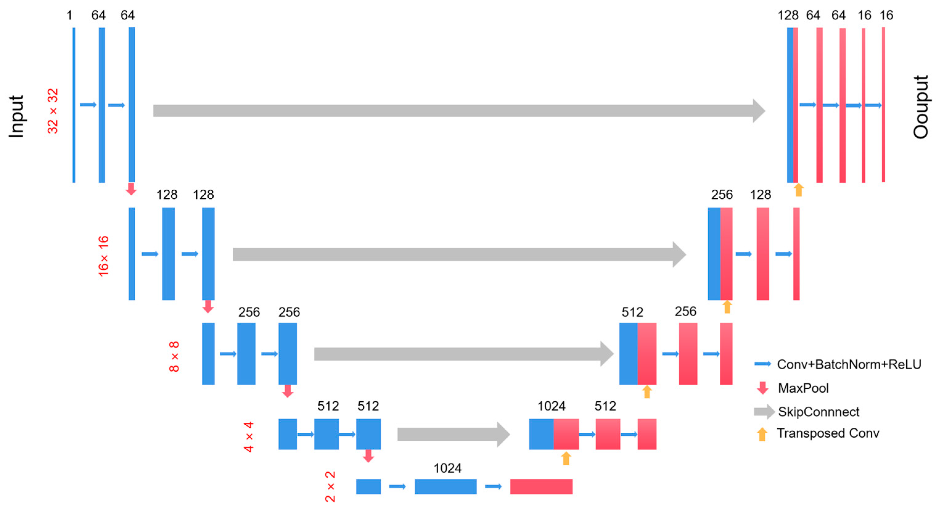
In this study, a U-Net network structure was used for deep learning, and a gravity forward modeling sample set was established for network training. As shown in Figure 1, the U-Net network is a typical full convolutional network (FCN), similar in shape to the letter “U”. The network is made up of two parts: one is the feature extraction layer on the left, also called the encoder, and the other is the upsampling process on the right, also called the decoder.
The left side of the network, the encoder, is a series of downsampling processes consisting of convolution and pooling. The whole consists of four submodules, each containing two convolutional layers, and each submodule is downsampled by a convolutional operation with a convolutional kernel of 2 × 2 and a step size of two. Also, a dropout layer is added to prevent overfitting.
The decoder is symmetrical to the encoder and also consists of four modules. It gradually learns features via upsampling until the output resolution matches the resolution of the input image. Meanwhile, a jump connection is used between the left and right parts to connect the upsampling result with the output of the submodule with the same resolution in the encoder, which is then used as the input of the next submodule in the decoder in order to obtain more accurate information and achieve better results.
The network uses batch learning; the batch size is 32, and the convolutional layers of the network are connected through the ELU activation function to increase the nonlinearity of the neural network and improve the ability of network learning and fitting. The optimizer selects Adam. Finally, the Tanh activation function is used to predict each pixel in the channel and generate the predicted subsurface density model. The above steps achieve the mapping of gravity data to the 3D prediction model via 2D-to-3D mapping. By modifying the number of input and output channels and the activation function, we can obtain a new network that can realize 3D-to-2D mapping.
Fine-tuning has become a common technique for using deep learning networks. When using deep networks for image processing tasks, using a model pretrained on a large data set to fine-tune its own data can often achieve better results than directly training on its own data because the model parameters pretrained on a large data set are in a better position from the beginning of the fine-tuning process and the fine-tuning can speed up the network convergence. When using large data sets for training, pretrained models have the ability to extract shallow basic features and deep abstract features. Without fine-tuning, training must begin from scratch, which requires a lot of data, computing time, and computing resources. In addition, risks such as model nonconvergence, insufficient parameter optimization, low accuracy, low generalization ability, and easy overfitting are present. Using fine-tuning can effectively avoid the above problems.
The process of fine-tuning involves initializing the built network with the trained parameters (obtained from the trained model) and then training with the data, adjusting the parameters in the same way as in the training process. For the initialization process, the constructed network is the target network, and the network corresponding to the trained model is the source network. The layer of the target network to be initialized should be the same as that of the source network (the name, type, and setting parameters of the layer are the same).
2.2. Self-Constrained Network
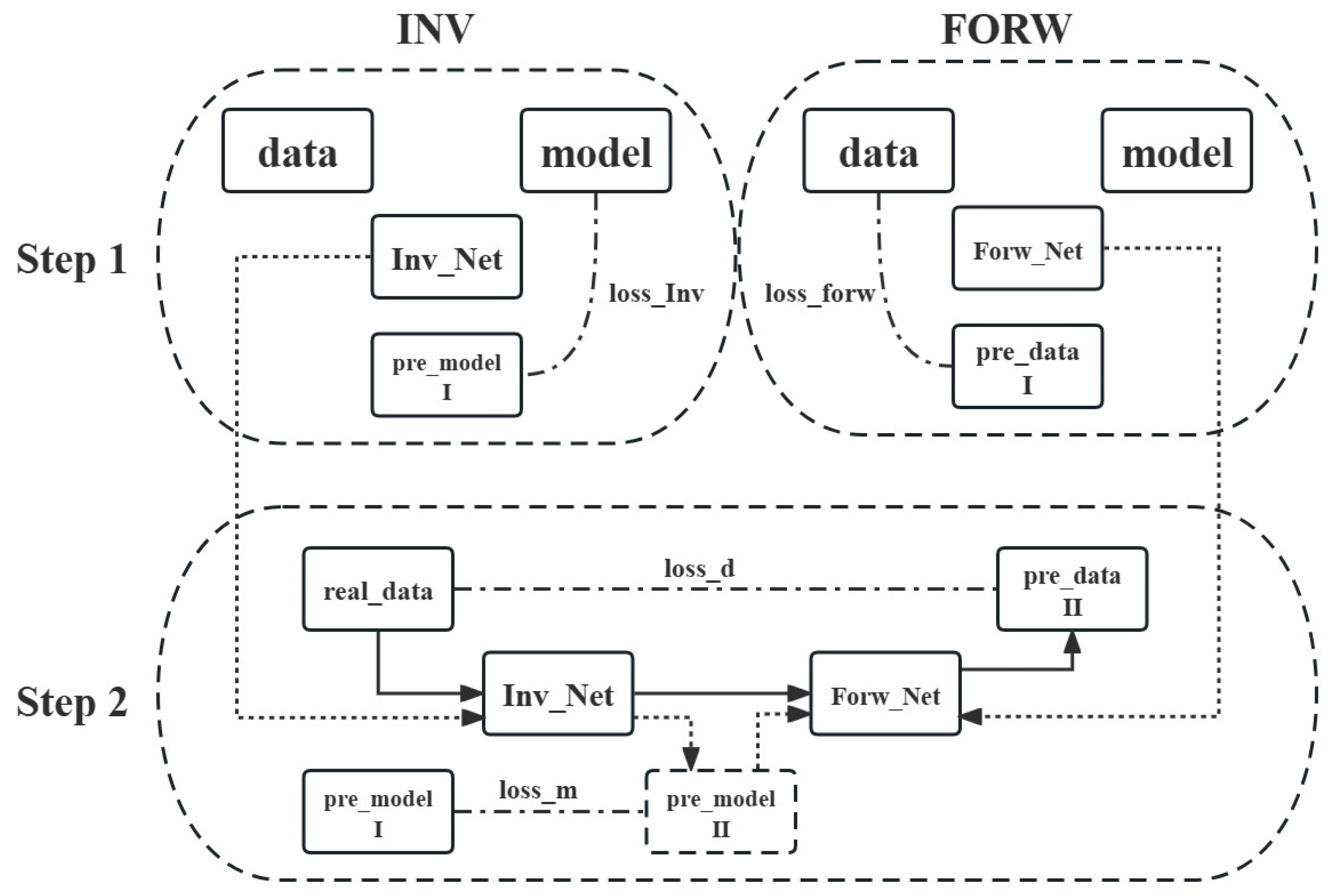
The data processing procedure used in this study is shown in Figure 2. The whole process is divided into two steps. The first step is to obtain two networks with good enough generalization using the data-driven deep learning method and realize 2D-to-3D and 3D-to-2D mapping. These two networks are called Inv_Net and Forw_Net. The second step is to build a new self-constrained network and introduce fine-tuning strategies based on data-driven deep learning so as to improve and optimize the prediction results obtained in the previous step, making them more reliable and accurate.
In the first step, we constructed a large number of random data sets to train the network in order to achieve strong generalization. When training Inv_Net, the input was 2D data, and the output was a 3D density model. In contrast, Forw_Net was trained with a 3D density model as the input and 2D gravity data as the output. The loss function of the two networks is defined as:
where and m represent the predicted models I and real models, and and d represent the predicted data I and true gravity data, respectively.
For traditional geophysical forward modeling, which typically divides the entire subsurface into N equally sized cubes, each with defined physical properties, the forward modeling of gravity anomalies can be expressed as:
where d represents the observed gravity anomaly data vector, m represents the residual density value vector of the model, and S represents the forward operator.
Because of their powerful nonlinear mapping capabilities, deep neural networks can represent any complex function. Therefore, once the mapping relationship of the neural network has been determined, it can be used to perform fast mapping to move from one thing to its corresponding other thing. In this paper, a U-Net network was used to approximate the forward modeling process and map the 3D gravity density model to the 2D gravity data, which can be expressed as:
where d represents the predicted gravity data, m represents the density model, F represents the forward network, and represents the parameters that the forward network needs to learn.
Forw_Net implements the above process of mapping a 3D density model to the 2D gravity data. By building large random data sets for training, Forw_Net can achieve high accuracy and be much faster.
The second step is the establishment of a self-constrained network and the introduction of the fine-tuning strategy. The process of fine-tuning involves initializing the built network with trained parameters (obtained from the trained model) and then training with the data, adjusting the parameters in the same way as in the training process. For the initialization process, the constructed network can be called the target network, and the network corresponding to the trained model is the source network. The layer of the target network to be initialized should be the same as that of the source network (the name, type, and setting parameters of the layer are the same).
In this study, the second step connected the same two networks as in the first step and initialized them. Therefore, the networks in the first step were the source networks, while the network in the second step was the target network. The input of the self-constrained network was 2D gravity data, and the output was also 2D gravity data, but the 3D density model can be output in the intermediate process. The network model parameters trained in the first step were loaded into the self-constrained network, and then the network was trained. Because the pretrained model has a strong enough generalization, that is, it has learned enough features, instead of retraining the entire network, certain layers can be fine-tuned. The specific approach was used to freeze the feature extraction portion and fine-tune the remaining layers using a lower learning rate. The target data of the second step were the unlabeled data, that is, the actual measured data. In order to obtain the labels required for supervised learning, the first step is to obtain a basic predicted model through the inversion network and fine-tune and improve on this basis. In this case, the loss function was defined as:
where, and represent the predicted model II and predicted model I, respectively, and and d represent the predicted data II and true gravity data, respectively. The second fine-tuning process involves the improvement and optimization of the generalization inversion results, so only a small amount of data is required. Meanwhile, the forward data fitting constraint was added so that the fine-tuning results were not only optimized in the inversion results but also had better forward fitting. The second step was the improvement and optimization of the results of the generalization inversion, so only a small amount of data was required. At the same time, a self-constrained control was added so that the fine-tuning results were not only optimized on the inversion results but also had better forward-fitting accuracy.
3. Model Testing
3.1. Data Set
In this study, the label was synthesized first, and then the corresponding input data were derived; that is, the density model was generated first, and then the synthetic data were calculated. In order to ensure the feasibility and effectiveness of deep learning inversion methods, the data set needs to be sufficiently complex. Therefore, we used random walks to generate a large number of relatively regular and diversified density models.
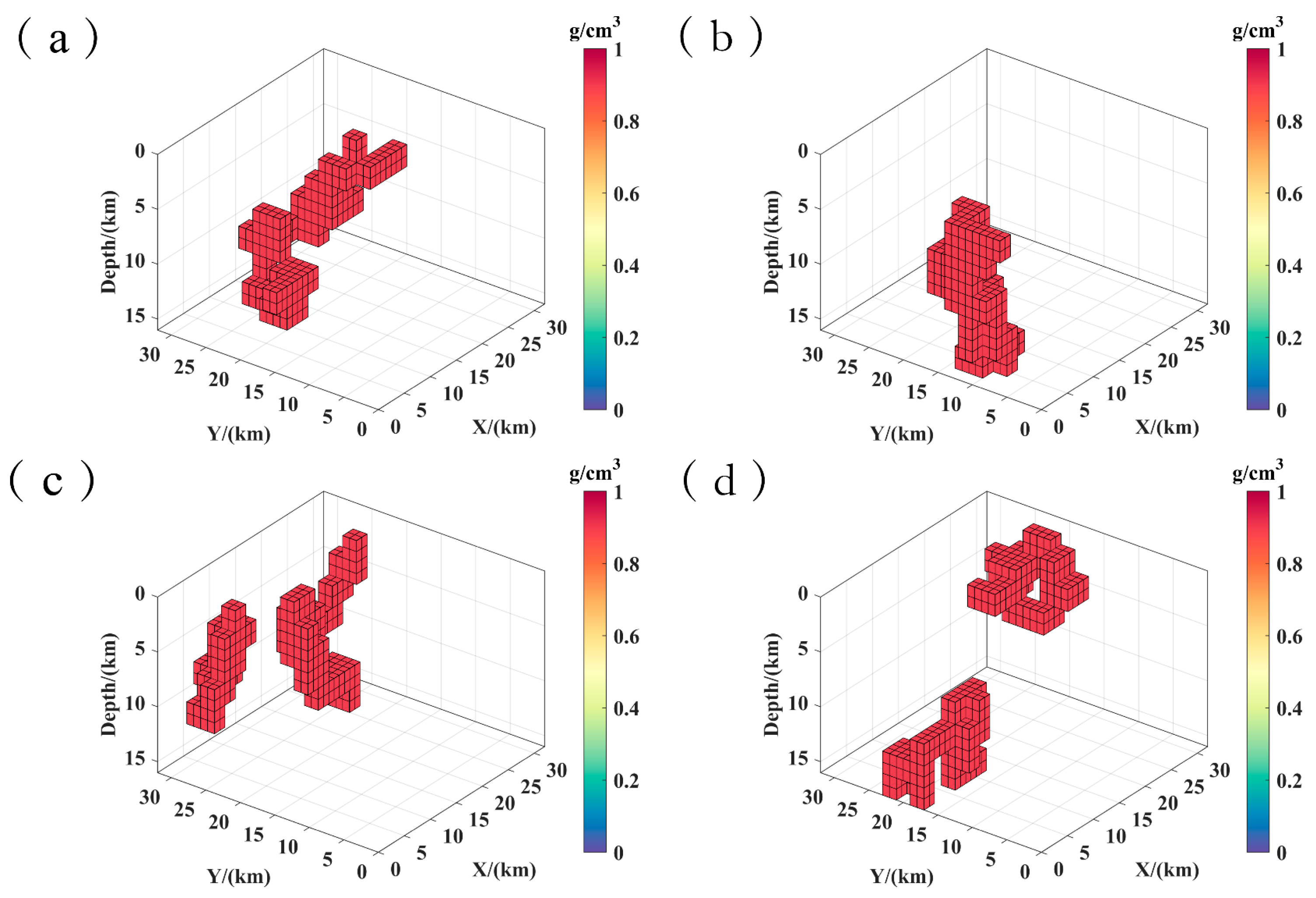
The subsurface research area was evenly divided into 32 × 32 × 16 = 16,384 cubes with a side length of 1 km, and then the subsurface density model was generated using a random walking method; that is, one or two starting points were randomly set in the space, and then they moved a certain number of steps in a random direction. When the actual model was established, the residual density of the gravity source was 1 g/cm3, and the background was 0 g/cm3. The density model was then generated in a 32 × 32 × 16 km subsurface area. In the subsurface area, one or two starting points were randomly set, and each starting point was composed of 8 cubes (2 × 2 × 2 km). The starting point randomly moved one step (2 km) in one direction (up, down, left, right, back, or forth), and the total number of steps of each starting point was 60–80, leading to a random model being generated in the space. Figure 3 shows some of the random models generated by this method, including models with one and two starting points.
For an observation point (x, y, z) on the ground, the gravity anomaly generated by each prism can be expressed as [30]:
where p, q, s = 1, 2. ,() is the coordinate of the prism. represents the universal gravitation constant, represents the residual density of the jth small prism, and represents the distance from the corner of the small prism to the observation point.
The gravity anomaly at the observation point can be expressed as the combined action of all underground prisms as follows:
where represents the kernel matrix of the jth small prism for the observation point. According to the above formula, the gravity data corresponding to each model can be calculated, and then the data set can be built.
The 30,000 data sets generated by the random walk method served as the training set and the verification set, while the test set consisted of a series of regular models containing 1000 data sets. The model’s physical properties of the training set, the verification set, and the test set were the same, and the ratio was 22:8:1. The 3D density model and its gravity data were used as data sets to train the two networks in the first step until a network model with strong generalization and high accuracy was obtained. The model parameters were then loaded into the network in step 2 for fine-tuning.
3.2. Model Testing
In order to prove the effectiveness of the proposed method and its advantages over data-driven deep learning methods, a series of models was used for testing, and the spatial position information of the models is shown in Table 1.
3.2.1. Model I
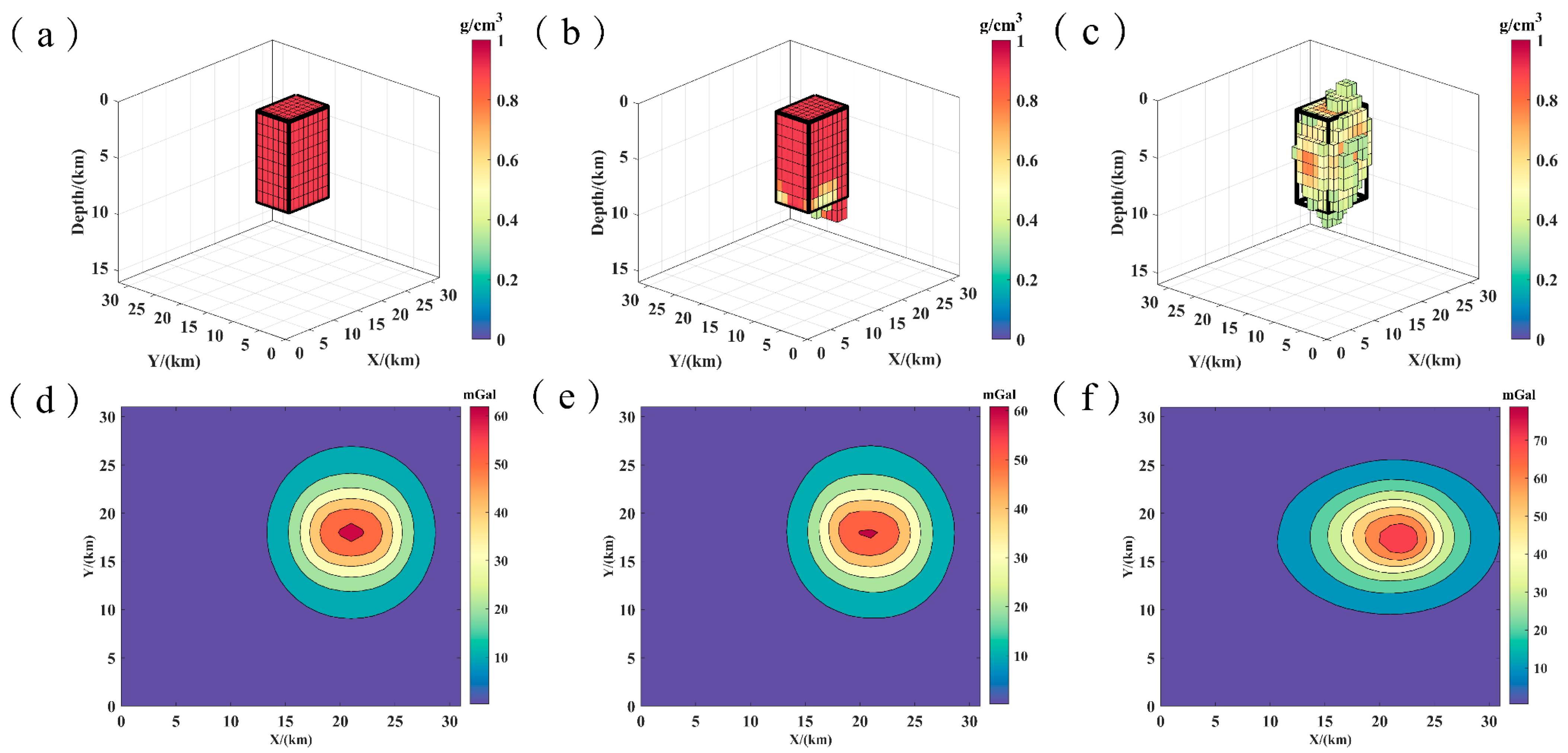
The model I was a single prism with a length of 8 km, a width of 6 km, and a height of 6 km, as shown in Figure 4a. Figure 4b shows the inversion results output by the fine-tuned inversion network, and the black solid line is the boundary of the real model. Figure 4c shows the inversion results of the data-driven deep learning method. It can be seen from the results that, compared with Figure 4c, the fine-tuned inversion network obtained a more focused 3D distribution of physical properties in the recovery of the physical parameters of the target body and the delineation of 3D spatial positions. Figure 4d–f show the gravity anomaly data corresponding to (a), (b), and (c), respectively. The results show that the degree of the network fitting to the observed data was improved because of the addition of self-constraint, and the fine-tuned inversion result obtained better data fitting accuracy.
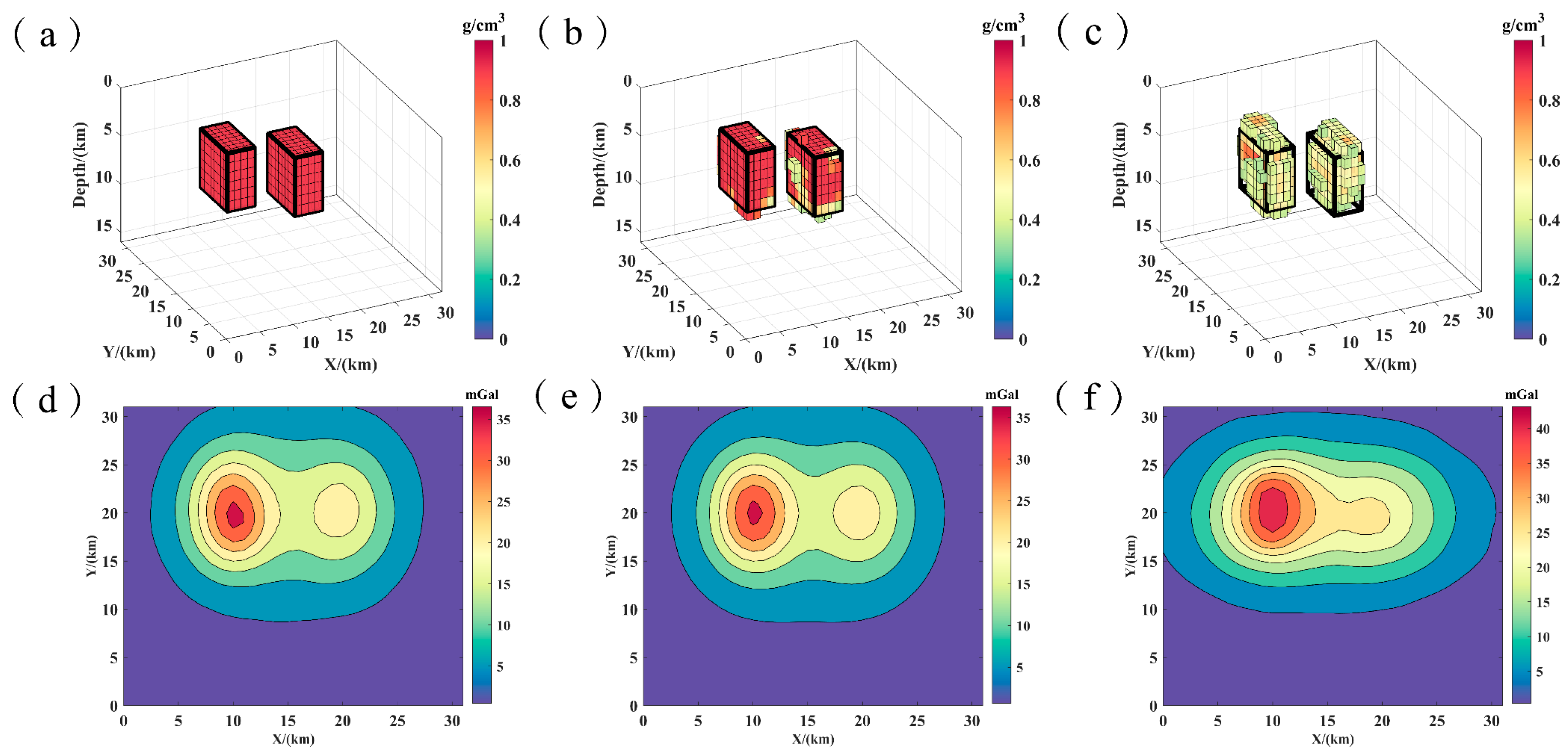
3.2.2. Model II
In order to test the effect of the inversion method on adjacent superimposed objects, model II was designed, as shown in Figure 5a. Model II consisted of two identical prisms with a length, width, and height of 8, 4, and 6 km, respectively, with a difference of 2 km in depth and 6 km in the Y direction. Figure 6b is the inversion output result of the fine-tuned inversion network, and the black solid line is the boundary of the real model. Figure 5c shows the inversion results of the data-driven deep learning method. It can be seen that the method can reverse the spatial position of the prisms but showed poor recovery of density values and fitting of boundary positions. However, the fine-tuned inversion results clearly reversed the 3D space positions of the two adjacent superimposed prisms, indicating that the proposed method has higher precision and resolution in the inversion of adjacent superimposed anomalous bodies. In forward data fitting, the fitting degree of the fine-tuned inversion results is much better because of the addition of the self-constraint, which makes the results obtained by the fine-tuned method more consistent with the forward theory of the gravity field.
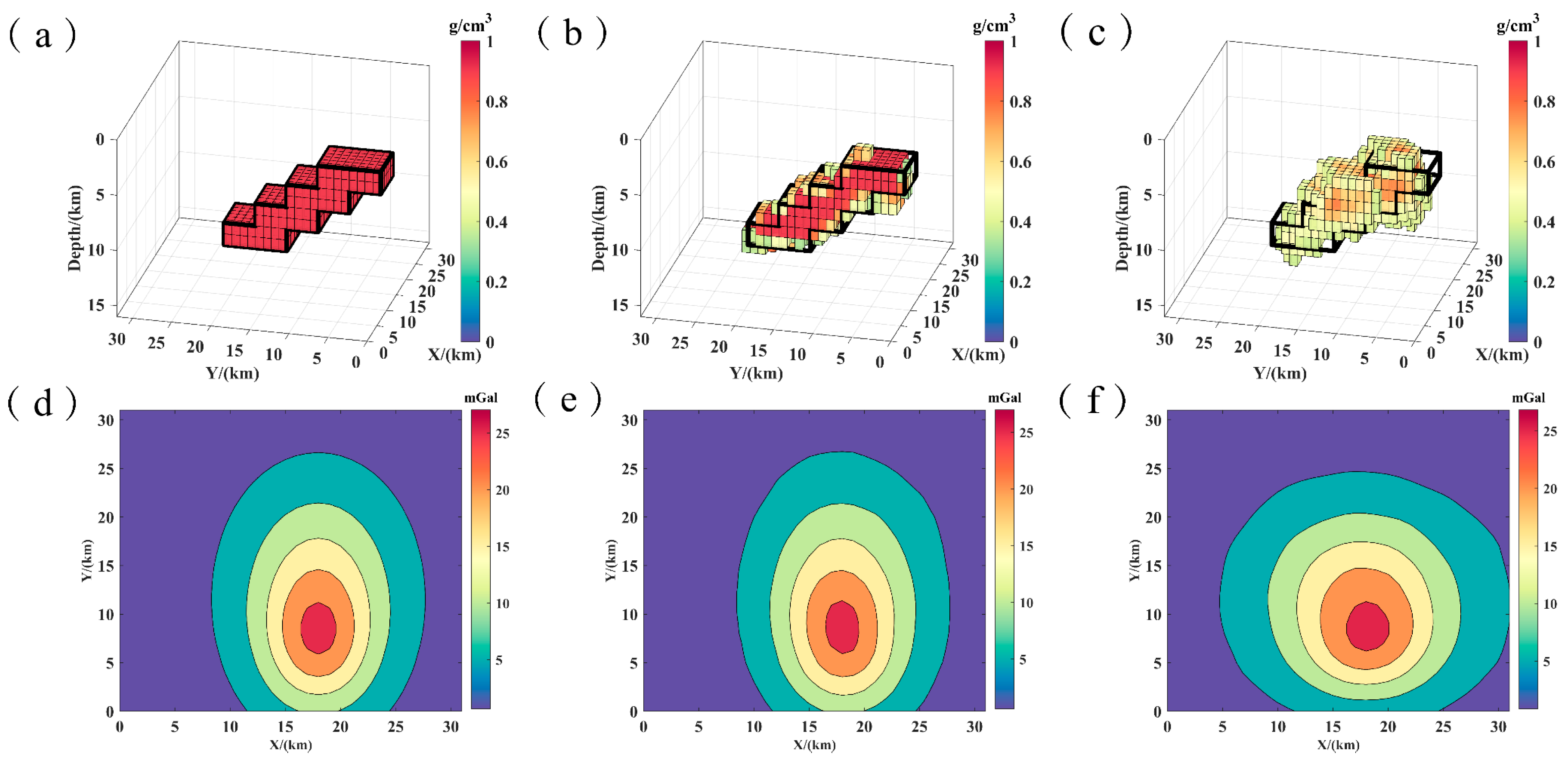
3.2.3. Model III
As shown in Figure 6a, model III was composed of four small prisms with a length, width, and height of 8, 4, and 2 km, respectively, with a total length of 20 km. Figure 6b shows the fine-tuned inversion results, and the black solid line is the boundary of the real model. Figure 6c shows the inversion results for the data-driven deep learning method. It can be seen that the fine-tuned inversion results obtained the model’s incline information, that the boundary delineation was closer to the true boundary, and that the boundary fitting accuracy was higher at the top and bottom of the target. In the recovery of physical property parameters, the inversion density value of the fine-tuned inversion results was obviously closer to the real density. The inversion results for the data-driven deep learning method were clearly inferior to the fine-tuned results. In the fitting of forward data, the fitting precision of the fine-tuned inversion results was obviously higher. This shows that the fine-tuning method can effectively invert the subsurface-inclined anomaly, which not only has a good effect on model reconstruction but also leads to excellent performance in forward fitting.
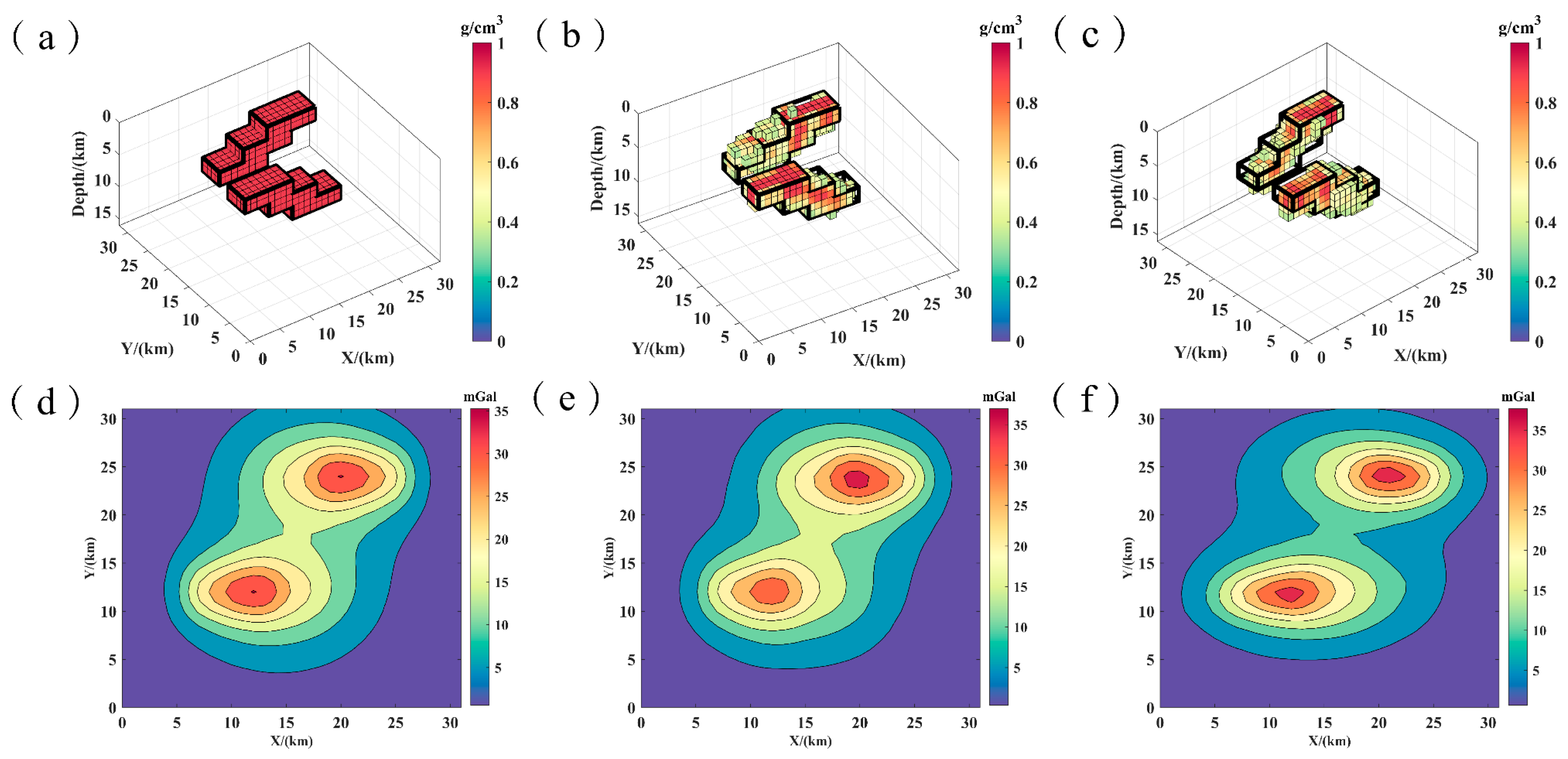
3.2.4. Model IV
As shown in Figure 7a, model IV was composed of two inclined steps of the same shape but opposite directions. Each inclined step was composed of three small prisms with a length, width, and height of 8, 4, and 2 km, respectively, with a total length of 16 km. The two inclined steps had the same depth, were opposite in the Y direction, and 8 km apart in the X direction. Figure 7b shows the fine-tuned inversion results, and the black solid line is the boundary of the real model. Figure 7c shows the inversion results of the data-driven deep learning method. It can be seen that the fine-tuned inversion results still obtained the model’s incline information under more complex conditions and are closer to the true boundary in the oblique boundary demarcation along the Y direction. Meanwhile, in the recovery of physical property parameters, the inversion density value of the fine-tuned inversion results was also significantly closer to the true density. Similarly, the forward data of the inversion results still had good fitting accuracy.
3.2.5. Analytical Metrics
In order to explain more specifically, the effect of inversion results, the root-mean-square error (RMSE) was introduced to conduct a quantitative analysis of the error between the model and the data. The expression is as follows:
In the formula, and represent the inversion results and their forward data, and and represent the real model and gravity data. and are used to represent the model fitting error and data fitting error, respectively. The closer the value is to 0, the better the model fitting is and the smaller the data fitting error is. Next, we undertook a quantitative analysis of the above four theoretical models, and the results are shown in Table 2.
4. Application of Field Data
Geothermal energy is the third largest renewable energy resource in the world. Dry, hot rocks are important geothermal resources, referring to rock bodies with temperatures higher than 180 °C and very low fluid content, whose thermal energy can be utilized by existing technologies. At present, their reserves are relatively abundant in the world, and it is generally believed that dry, hot rocks are mainly stored about 3–10 km underground. For these rocks to be utilized by humans, they need to have several characteristics, such as high temperature, shallow burial depth, and low development and utilization difficulty and cost. According to a statistical report released by the Massachusetts Institute of Technology in 2006, dry, hot rock reserves are extremely abundant in the world, and the energy of dry, hot rock reserves at a depth of 3–10 km underground is equivalent to nearly 3000 times the total energy consumption of the United States in 2005 [31].
Gonghe Basin is located in an area with significantly concentrated geothermal activities and features significant geothermal anomalies, with a high heat flow value of 90 to 300 mW/m2 [32]. The Gonghe Basin is not only rich in hydrothermal geothermal resources but is also one of the areas with the most potential for the development of hot, dry rock geothermal resources in China. It has been shown that the average geothermal gradient in the Republican Basin is more than double the standard geothermal gradient [33].
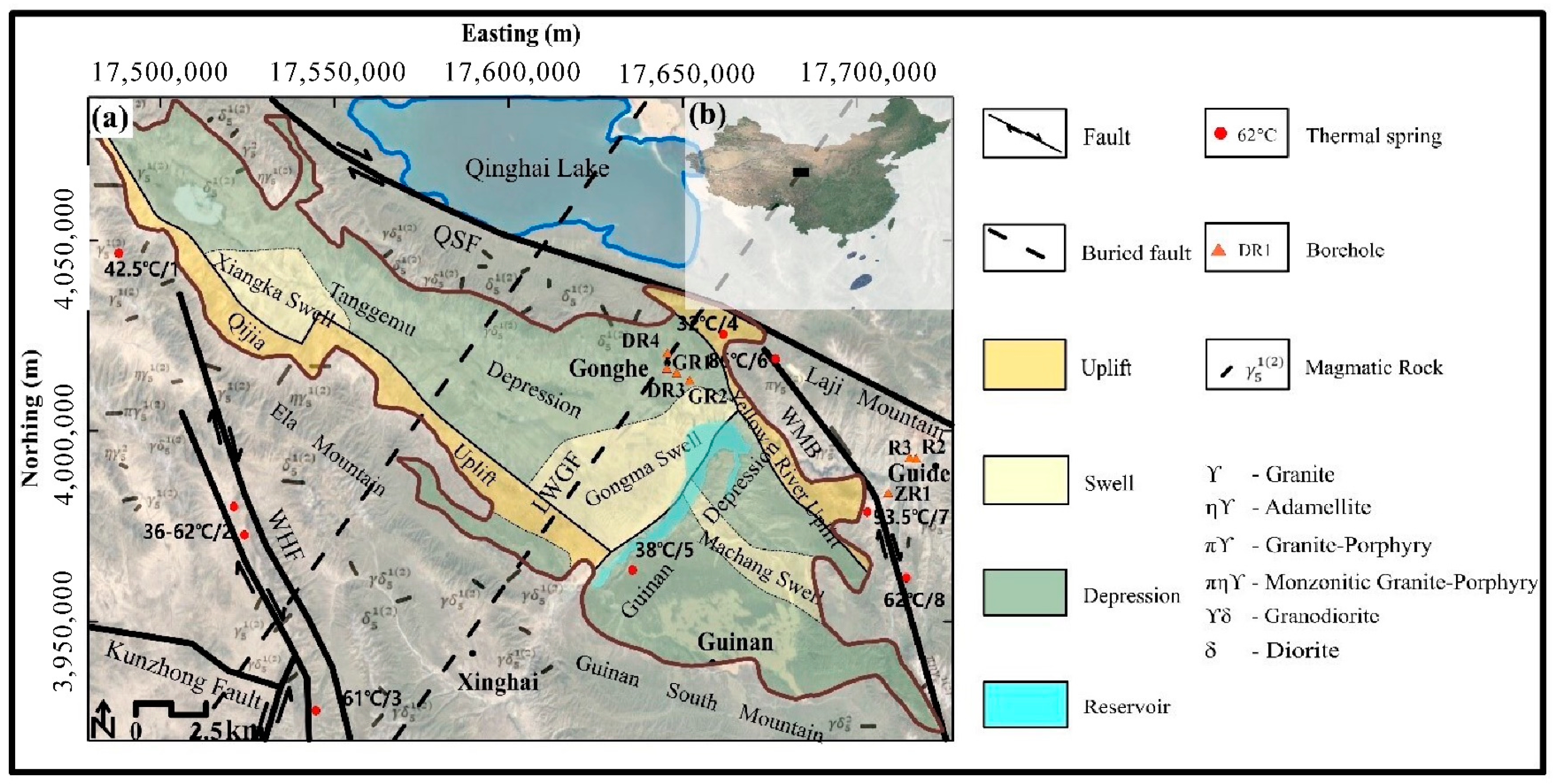
Gonghe Basin, the third largest basin in Qinghai Province, is about 280 km long and 95 km wide. It covers an area of about 15,000 km2 and has a diamond distribution shape. As shown in Figure 8, located in the northeast margin of the Qinghai–Tibet Plateau, the Gonghe Basin is surrounded by several tectonic belts, orogenic belts, and faults. The west side of the basin is bounded by the Wahongshan strike-slip fault and Qaidam–East Kunlun fault and is adjacent to the West Qinling block. On the east side, the basin is bounded by the Duohemao Fault and adjacent to the Bayankela Basin. The southern part of the basin is bounded by the Anyemakeng suture belt and adjacent to the Songpan–Garze fold belt, while the northern part of the basin is bounded by the Qinghai Lake Nanshan Fault and adjacent to the Qilian orogenic belt. It is the most intense deformation area of the Qinghai–Tibet Plateau since the late Cenozoic [34,35,36]. Subject to plate collision, the northeastern part of the Qinghai–Tibetan Plateau is still in the stage of deformation and is currently undergoing continuous uplift. Because of the existence of ruptures, the geological structure of the surrounding area has become very complex, structurally heterogeneous, and unstable, so the Gonghe Basin area has strong tectonic activity [37].
A complete geothermal system consists of three main components: a cap rock, a heat reservoir, and a heat source. Gao et al. also analyzed and discussed the three components of the Gonghe Basin using 3D magnetotelluric imaging [39]. The results show that the resistivity near the surface is very low, which corresponds well with the deposited material. The cap rock of a geothermal system is generally a low-permeability layer, which mainly prevents heat loss. The cap rock in the Gonghe Basin corresponds to Quaternary sediments with a thickness of 700 to 1600 m. Previous research has focused on the basin’s heat sources, with two large low-resistivity anomalies at depths of 15 to 35 km being found. Combined with the relevant data, it can be inferred that this area is composed of a molten body, which is the heat source of the geothermal system in the Gonghe Basin. The 3D resistivity model also showed a general low-resistivity anomaly beginning at a depth of 3 km, which was interpreted as a reservoir of the Gonghe Basin geothermal system.
Hirt et al. obtained the distribution of ultrahigh-resolution gravity anomalies in this region, showing that this region is associated with low-gravity anomalies [40]. This indicates the presence of low-density rock formations below the study area. As the temperature rises, the seismic speed and density of the rock decrease [39]. Therefore, the inversion of gravity data in this area can predict the distribution of underground heat reservoirs.
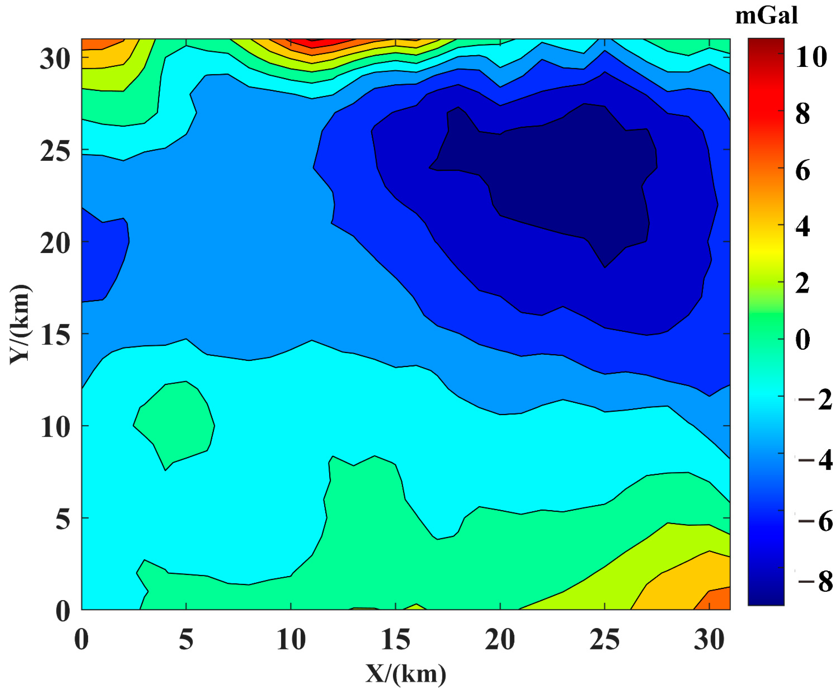
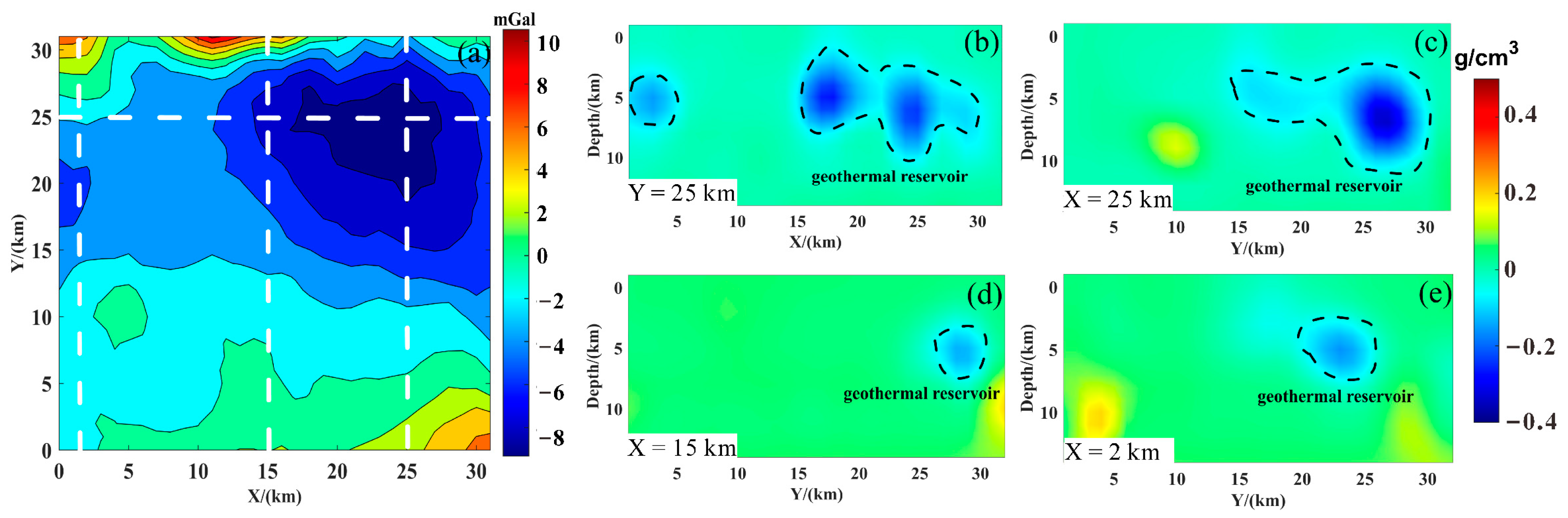
Figure 9 shows the gravity anomaly data collected in the Gonghe Basin. In order to prove the effectiveness of our method in real situations and detect the distribution of heat reservoirs, we applied it to the Gonghe Basin region. Using the trained network model, we processed the gravity data and divided the subsurface space into 32 × 32 × 16 = 16,384 prisms. According to the process, the gravity data were first input into the inversion network, and the preliminary prediction model was obtained. Then, the gravity data and preliminary prediction model were input into the self-constrained network, and 3D inversion results were obtained after prediction. In order to clearly display the inversion result, four cross sections were selected, as shown in Figure 10b–e. The white dotted line in Figure 10a is the location of the four profiles, and the black dotted line in Figure 10b–e is the geothermal reservoir. They clearly show a wide range of negative density anomalies in the subsurface, with depths ranging from approximately 3 to 10 km. This is consistent with the results obtained by Gao et al., indicating that the distribution of heat reservoir is roughly within this range. The results also showed that the subsurface negative density anomalies are mainly distributed in the east and the west. The scale of the negative density anomalies is larger in the east, and there are also smaller negative density anomalies in the west. This indicates that there are also small reserves in the west. The 3D inversion results were generally effective in mapping geothermal storage areas, which indicates that the inversion method has a good effect on the actual data processing and interpretation.
5. Conclusions
In this paper, a deep learning gravity inversion method based on a self-constrained network was proposed. On the basis of the data-driven deep learning gravity inversion method, a new inversion idea was proposed, and a fine-tuning strategy was introduced. Through the control of the self-constrained network, the inversion results were improved in the forward data fitting. At the same time, because of the introduction of a fine-tuning strategy, the inversion results could be optimized and improved. Through model testing, we verified the effectiveness of this method, and the inversion results showed good performance in model fitting and data fitting. Finally, the method was applied to the gravity data inversion of the Gonghe Basin in Qinghai Province, and reasonable results were obtained.
It is worth noting that the fine-tuning process was based on the pretrained network model, so the generalization and accuracy of the pretrained model must be guaranteed. This means that the number and richness of data sets for pretraining needs to be guaranteed. The method proposed in this paper is not only suitable for gravity inversion but also feasible for other geophysical methods. In addition, if there are other prior information constraints, they can be added to the proposed method.
Author Contributions
Conceptualization, S.Z.; methodology, P.L.; writing, Y.W.; supervision, J.J. and J.Z.; project administration, P.Y., G.Y. and S.W.; All authors have read and agreed to the published version of the manuscript.
Funding
This work was supported in part by the Ningxia Key R&D Plan under Grant 2023BEG02066, the National Natural Science Foundation of China under Grant 42204141 and Grant 42074119, and the Fundamental Research Funds for the Central Universities under Grant 2023-JCXK-15, and the scientific research project of Education Department of Jilin Province (JJKH20241293KJ).
Data Availability Statement
Not applicable.
Acknowledgments
The author is grateful to Jianhao Jia, Meijing Xu, and Xinfei Li, Jilin University, for processing the actual data. The authors would like to thank the editors and reviewers for providing their valuable comments and suggestions.
Conflicts of Interest
The authors declare no conflicts of interest.
References
- Geng, M.; Huang, D.; Yang, Q.; Liu, Y. 3D inversion of airborne gravity-gradiometry data using cokriging. Geophysics 2014, 79, G37–G47. [Google Scholar] [CrossRef]
- Li, Y.; Oldenburg, D.W. 3-D inversion of gravity data. Geophysics 1998, 63, 109–119. [Google Scholar] [CrossRef]
- Montesinos, F.G.; Arnoso, J.; Vieira, R. Using a genetic algorithm for 3-D inversion of gravity data in Fuerteventura (Canary Islands). Int. J. Earth Sci. 2005, 94, 301–316. [Google Scholar] [CrossRef]
- Liu, S.; Hu, X.; Liu, T. A Stochastic Inversion Method for Potential Field Data: Ant Colony Optimization. Pure Appl. Geophys. 2013, 171, 1531–1555. [Google Scholar] [CrossRef]
- Liu, S.; Liang, M.; Hu, X. Particle swarm optimization inversion of magnetic data: Field examples from iron ore deposits in China. Geophysics 2018, 83, J43–J59. [Google Scholar] [CrossRef]
- Al-Garni, M.A. Inversion of residual gravity anomalies using neural network. Arab. J. Geosci. 2011, 6, 1509–1516. [Google Scholar] [CrossRef]
- Guspí, F. Noniterative nonlinear gravity inversion. Geophysics 1993, 58, 935–940. [Google Scholar] [CrossRef]
- Qin, P.; Huang, D.; Yuan, Y.; Geng, M.; Liu, J. Integrated gravity and gravity gradient 3D inversion using the non-linear conjugate gradient. J. Appl. Geophys. 2016, 126, 52–73. [Google Scholar] [CrossRef]
- Uieda, L.; Barbosa, V.C. Fast nonlinear gravity inversion in spherical coordinates with application to the South American Moho. Geophys. J. Int. 2016, 208, 162–176. [Google Scholar] [CrossRef]
- Wang, J.; Meng, X.; Li, F. Fast Nonlinear Generalized Inversion of Gravity Data with Application to the Three-Dimensional Crustal Density Structure of Sichuan Basin, Southwest China. Pure Appl. Geophys. 2017, 174, 4101–4117. [Google Scholar] [CrossRef]
- Bhangale, K.B.; Kothandaraman, M. Survey of Deep Learning Paradigms for Speech Processing. Wirel. Pers. Commun. 2022, 125, 1913–1949. [Google Scholar] [CrossRef]
- Lin, Y.; Wu, Y. InversionNet: A real-time and accurate full waveform inversion with convolutional neural network. J. Acoust. Soc. Am. 2018, 144, 1683. [Google Scholar] [CrossRef]
- Ren, Y.; Nie, L.; Yang, S.; Jiang, P.; Chen, Y. Building Complex Seismic Velocity Models for Deep Learning Inversion. IEEE Access 2021, 9, 63767–63778. [Google Scholar] [CrossRef]
- Liu, B.; Yu, A.; Yu, X.; Wang, R.; Gao, K.; Guo, W. Deep Multiview Learning for Hyperspectral Image Classification. IEEE Trans. Geosci. Remote Sens. 2021, 59, 7758–7772. [Google Scholar] [CrossRef]
- Ren, Y.; Xu, X.; Yang, S.; Nie, L.; Chen, Y. A Physics-Based Neural-Network Way to Perform Seismic Full Waveform Inversion. IEEE Access 2020, 8, 112266–112277. [Google Scholar] [CrossRef]
- Zhang, L.; Zhang, G.; Liu, Y.; Fan, Z. Deep Learning for 3-D Inversion of Gravity Data. IEEE Trans. Geosci. Remote Sens. 2022, 60, 5905918. [Google Scholar] [CrossRef]
- Huang, R.; Liu, S.; Qi, R.; Zhang, Y. Deep Learning 3D Sparse Inversion of Gravity Data. J. Geophys. Res. Solid Earth 2021, 126, e2021JB022476. [Google Scholar] [CrossRef]
- Wang, Y.-F.; Zhang, Y.-J.; Fu, L.-H.; Li, H.-W. Three-dimensional gravity inversion based on 3D U-Net++. Appl. Geophys. 2021, 18, 451–460. [Google Scholar] [CrossRef]
- Hu, Z.; Liu, S.; Hu, X.; Fu, L.; Qu, J.; Wang, H.; Chen, Q. Inversion of magnetic data using deep neural networks. Phys. Earth Planet. Inter. 2021, 311, 106653. [Google Scholar] [CrossRef]
- Zhang, S.; Zhang, S.; Yin, C.; Yin, C.; Cao, X.; Cao, X.; Sun, S.; Sun, S.; Liu, Y.; Liu, Y.; et al. DecNet: Decomposition network for 3D gravity inversion. Geophysics 2022, 87, G103–G114. [Google Scholar] [CrossRef]
- Yang, Q.; Hu, X.; Liu, S.; Jie, Q.; Wang, H.; Chen, Q. 3-D Gravity Inversion Based on Deep Convolution Neural Networks. IEEE Geosci. Remote Sens. Lett. 2022, 19, 3001305. [Google Scholar] [CrossRef]
- Singh, S.; Zhang, Y.; Thanoon, D.; Devarakota, P.R.; Jin, L.; Tsvankin, I. Physics-directed unsupervised machine learning: Quantifying uncertainty in seismic inversion. In Second International Meeting for Applied Geoscience & Energy; SEG Technical Program Expanded Abstracts; Society of Exploration Geophysicists: Houston, TX, USA, 2022; pp. 1735–1739. [Google Scholar] [CrossRef]
- Su, Y.; Cao, D.; Liu, S.; Hou, Z.; Feng, J. Seismic impedance inversion based on deep learning with geophysical constraints. Geoenergy Sci. Eng. 2023, 225, 211671. [Google Scholar] [CrossRef]
- Zhang, J.; Li, J.; Chen, X.; Li, Y.; Huang, G.; Chen, Y. Robust deep learning seismic inversion with a priori initial model constraint. Geophys. J. Int. 2021, 225, 2001–2019. [Google Scholar] [CrossRef]
- Wang, Y.; Wang, Q.; Lu, W.; Li, H. Physics-Constrained Seismic Impedance Inversion Based on Deep Learning. IEEE Geosci. Remote Sens. Lett. 2022, 19, 7503305. [Google Scholar] [CrossRef]
- Hansen, T.M.; Cordua, K.S. Efficient Monte Carlo sampling of inverse problems using a neural network-based forward—Applied to GPR crosshole traveltime inversion. Geophys. J. Int. 2017, 211, 1524–1533. [Google Scholar] [CrossRef]
- Conway, D.; Alexander, B.; King, M.; Heinson, G.; Kee, Y. Inverting magnetotelluric responses in a three-dimensional earth using fast forward approximations based on artificial neural networks. Comput. Geosci. 2019, 127, 44–52. [Google Scholar] [CrossRef]
- Moghadas, D.; Behroozmand, A.A.; Vest Christiansen, A. Soil electrical conductivity imaging using a neural network-based forward solver: Applied to large-scale Bayesian electromagnetic inversion. J. Appl. Geophys. 2020, 176, 104012. [Google Scholar] [CrossRef]
- Lv, M.; Zhang, Y.; Liu, S. Fast forward approximation and multitask inversion of gravity anomaly based on UNet3+. Geophys. J. Int. 2023, 234, 972–984. [Google Scholar] [CrossRef]
- Boulanger, O.; Chouteau, M. Constraints in 3D gravity inversion. Geophys. Prospect. 2001, 49, 265–280. [Google Scholar] [CrossRef]
- Zarrouk, S.J.; Moon, H. Efficiency of geothermal power plants: A worldwide review. Geothermics 2014, 51, 142–153. [Google Scholar] [CrossRef]
- Tang, X.; Zhang, J.; Pang, Z.; Hu, S.; Tian, J.; Bao, S. The eastern Tibetan plateau geothermal belt, western China: Geology, geophysics, genesis, and hydrothermal system. Tectonophysics 2017, 717, 433–448. [Google Scholar] [CrossRef]
- Liu, W.L. Drilling technical difficulties and solutions in development of Hot dry Rock geothermal energy. Adv. Pet. Explor. Dev. 2017, 13, 63–69. [Google Scholar]
- Feng, Y.M.; Cao, X.D.; Zhang, E.P.; Hu, Y.X.; Pan, X.P.; Yang, J.L. Tectonic evolution framework and nature of the west Qinling orogenic belt. Northwestern Geol. 2003, 1, 1–10. [Google Scholar]
- Zhang, H.; Chen, Y.; Xu, W.C.; Liu, R.; Yuan, H.-L.; Liu, X. Granitoids around Gonghe basin in Qinghai province: Petrogenesis and tectonic implications. Acta Petrol. Sin. 2006, 22, 2910–2922. [Google Scholar]
- Fang, X.; Yan, M.; Van der Voo, R.; Rea, D.K.; Song, C.; Parés, J.M.; Gao, J.; Nie, J.; Dai, S. Late Cenozoic deformation and uplift of the NE Tibetan Plateau: Evidence from high-resolution magnetostratigraphy of the Guide Basin, Qinghai Province, China. GSA Bull. 2005, 117, 1208–1225. [Google Scholar] [CrossRef]
- Zhao, X.; Zeng, Z.; Wu, Y.; He, R.; Wu, Q.; Zhang, S. Interpretation of gravity and magnetic data on the hot dry rocks (HDR) delineation for the enhanced geothermal system (EGS) in Gonghe town, China. Environ. Earth Sci. 2020, 79, 390. [Google Scholar] [CrossRef]
- Wang, Z.; Zeng, Z.; Liu, Z.; Zhao, X.; Li, J.; Bai, L.; Zhang, L. Heat Flow Distribution and Thermal Mechanism Analysis of the Gonghe Basin based on Gravity and Magnetic Methods. Acta Geol. Sin. 2021, 95, 1892–1901. [Google Scholar] [CrossRef]
- Gao, J.; Zhang, H.; Zhang, S.; Chen, X.; Cheng, Z.; Jia, X.; Li, S.; Fu, L.; Gao, L.; Xin, H. Three-dimensional magnetotelluric imaging of the geothermal system beneath the Gonghe Basin, Northeast Tibetan Plateau. Geothermics 2018, 76, 15–25. [Google Scholar] [CrossRef]
- Hirt, C.; Claessens, S.; Fecher, T.; Kuhn, M.; Pail, R.; Rexer, M. New ultrahigh-resolution picture of Earth’s gravity field. Geophys. Res. Lett. 2013, 40, 4279–4283. [Google Scholar] [CrossRef]
Figure 1.
Network structure.

Figure 2.
The process of self-constraining the network.

Figure 3.
Random models. (a,b) are random models generated from one starting point, and (c,d) are random models generated from two starting points.
Figure 3.
Random models. (a,b) are random models generated from one starting point, and (c,d) are random models generated from two starting points.

Figure 4.
(a) Real model; (b) fine-tuned inversion results; (c) inversion results for data-driven deep learning method; (d) real anomaly data; (e,f) forward data of (b,c).
Figure 4.
(a) Real model; (b) fine-tuned inversion results; (c) inversion results for data-driven deep learning method; (d) real anomaly data; (e,f) forward data of (b,c).

Figure 5.
(a) Real model; (b) fine-tuned inversion results; (c) inversion results for data-driven deep learning method; (d) real anomaly data; (e,f) forward data of (b,c).
Figure 5.
(a) Real model; (b) fine-tuned inversion results; (c) inversion results for data-driven deep learning method; (d) real anomaly data; (e,f) forward data of (b,c).

Figure 6.
(a) Real model; (b) fine-tuned inversion results; (c) inversion results of data-driven deep learning method; (d) real anomaly data; (e,f) forward data of (b,c).
Figure 6.
(a) Real model; (b) fine-tuned inversion results; (c) inversion results of data-driven deep learning method; (d) real anomaly data; (e,f) forward data of (b,c).

Figure 7.
(a) Real model; (b) fine-tuned inversion results; (c) inversion results of data-driven deep learning method; (d) real anomaly data; (e,f) forward data of (b,c).
Figure 7.
(a) Real model; (b) fine-tuned inversion results; (c) inversion results of data-driven deep learning method; (d) real anomaly data; (e,f) forward data of (b,c).

Figure 8.
(a) Geological structure map of the Republican Basin and the surrounding area, with the study and inversion areas in red boxes (modified from Wang et al., 2021 [38]); (b) location of the study area.
Figure 8.
(a) Geological structure map of the Republican Basin and the surrounding area, with the study and inversion areas in red boxes (modified from Wang et al., 2021 [38]); (b) location of the study area.

Figure 9.
Gravity anomaly in the Gonghe area.

Figure 10.
Cross sections of 3D density model (b–e) along the profiles shown in (a).


Table 1.
The range of the models in the X, Y, and Z directions.
| Model | X/km | Y/km | Z/km |
|---|---|---|---|
| Model I | 17–25 | 15–21 | 2–10 |
| Model II | 8–12; 18–22 | 16–24 | 3–9; 5–11 |
| Model III | 15–21 | 2–22 | 5–13 |
| Model IV | 6–22; 10–26 | 10–14; 22–26 | 2–8 |
Table 2.
Error analysis of the models.
| Model | Data-Driven Deep Learning | Self-Constrained Network | ||
|---|---|---|---|---|
| Em | Ed | Em | Ed | |
| Model I | 10.2667 | 98.8648 | 7.2498 | 34.1445 |
| Model II | 10.3254 | 90.0130 | 8.2652 | 33.6362 |
| Model III | 15.3313 | 71.3274 | 11.5404 | 31.2421 |
| Model IV | 11.3257 | 54.6194 | 8.3752 | 42.3873 |
Disclaimer/Publisher’s Note: The statements, opinions and data contained in all publications are solely those of the individual author(s) and contributor(s) and not of MDPI and/or the editor(s). MDPI and/or the editor(s) disclaim responsibility for any injury to people or property resulting from any ideas, methods, instructions or products referred to in the content. |
© 2024 by the authors. Licensee MDPI, Basel, Switzerland. This article is an open access article distributed under the terms and conditions of the Creative Commons Attribution (CC BY) license (https://creativecommons.org/licenses/by/4.0/).
Share and Cite
MDPI and ACS Style
Zhou, S.; Wei, Y.; Lu, P.; Yu, G.; Wang, S.; Jiao, J.; Yu, P.; Zhao, J. A Deep Learning Gravity Inversion Method Based on a Self-Constrained Network and Its Application. Remote Sens. 2024, 16, 995. https://doi.org/10.3390/rs16060995
AMA Style
Zhou S, Wei Y, Lu P, Yu G, Wang S, Jiao J, Yu P, Zhao J. A Deep Learning Gravity Inversion Method Based on a Self-Constrained Network and Its Application. Remote Sensing. 2024; 16(6):995. https://doi.org/10.3390/rs16060995
Chicago/Turabian StyleZhou, Shuai, Yue Wei, Pengyu Lu, Guangrui Yu, Shuqi Wang, Jian Jiao, Ping Yu, and Jianwei Zhao. 2024. "A Deep Learning Gravity Inversion Method Based on a Self-Constrained Network and Its Application" Remote Sensing 16, no. 6: 995. https://doi.org/10.3390/rs16060995
Note that from the first issue of 2016, this journal uses article numbers instead of page numbers. See further details here.