
A Spatiotemporal Enhanced SMAP Freeze/Thaw Product (1980–2020) over China and Its Preliminary Analyses

State Key Laboratory of Earth Surface Processes and Resource Ecology, Faculty of Geographical Science, Beijing Normal University, Beijing 100875, China
*
Author to whom correspondence should be addressed.
Remote Sens. 2024, 16(6), 950; https://doi.org/10.3390/rs16060950
Submission received: 18 January 2024
/
Revised: 26 February 2024
/
Accepted: 6 March 2024
/
Published: 8 March 2024
(This article belongs to the Special Issue Advances in Deep Learning in the Retrieval of Key Parameters of Agrometeorological Remote Sensing)
Abstract
:The soil freeze/thaw (FT) state has emerged as a critical role in the ecosystem, hydrological, and biogeochemical processes, but obtaining representative soil FT state datasets with a long time sequence, fine spatial resolution, and high accuracy remains challenging. Therefore, we propose a decision-level spatiotemporal data fusion algorithm based on Convolutional Long Short-Term Memory networks (ConvLSTM) to expand the SMAP-enhanced L3 landscape freeze/thaw product (SMAP_E_FT) temporally. In the algorithm, the Freeze/Thaw Earth System Data Record product (ESDR_FT) is sucked in the ConvLSTM and fused with SMAP_E_FT at the decision level. Eight predictor datasets, i.e., soil temperature, snow depth, soil moisture, precipitation, terrain complexity index, area of open water data, latitude and longitude, are used to train the ConvLSTM. Direct validation using six dense observation networks located in the Genhe, Maqu, Naqu, Pali, Saihanba, and Shandian river shows that the fusion product (ConvLSTM_FT) effectively absorbs the high accuracy characteristics of ESDR_FT and expands SMAP_E_FT with an overall average improvement of 2.44% relative to SMAP_E_FT, especially in frozen seasons (averagely improved by 7.03%). The result from indirect validation based on categorical triple collocation also shows that ConvLSTM_FT performs stable regardless of land cover types, climate types, and terrain complexity. The findings, drawn from preliminary analyses on ConvLSTM_FT from 1980 to 2020 over China, suggest that with global warming, most parts of China suffer from different degrees of shortening of the frozen period. Moreover, in the Qinghai–Tibet region, the higher the permafrost thermal stability, the faster the degradation rate.
1. Introduction
Approximately 57% of the northern hemisphere’s land surface is seasonally frozen ground, and 25% is permafrost [1,2,3,4]. These conditions typically occur in cold regions, either at high altitudes or high latitudes, where temperatures are low. The soil freeze/thaw (FT) process, driven by diurnal or seasonal temperature changes, affects the surface of seasonally frozen ground and the active layer of permafrost. The ice-water phase transitions during the soil FT processes are accompanied by the absorption or release of massive latent heat, which not only plays an important role in regulating the surface energy balance but also directly affects the water cycle and the exchange of carbon between the atmosphere and the surface [5,6]. Studies indicate that, globally, frozen soils contain approximately 146 to 160 million tons of carbon [7,8]. This amount is nearly double the carbon present in the atmosphere and constitutes over half of the global soil carbon stock [9]. Recent decades of rapid global warming have resulted in the degradation of permafrost and a spatial extension of seasonally frozen ground, accompanied by a large amount of organic carbon being broken down by microbes and released into the atmosphere, further climate warming [10,11,12]. A large number of studies show that permafrost is degrading and will deteriorate or even disappear in the future [13,14,15]. This has a range of human social [16] and ecological [17,18] impacts. However, the current research on permafrost lacks long-term and large-scale continuous monitoring data. In addition, as a region with unique climatic characteristics, ecological environment and geographical location, the response of permafrost on the Qinghai–Tibet Plateau (QTP) to global warming is not only relevant to the future of the regional environment and social economy but also the key to understand the feedback mechanism of the Earth’s system in the context of global climate change. Therefore, a soil FT state dataset with a long time sequence, fine spatial resolution, and high accuracy will benefit the research about environmental science, climate change mitigation strategies, and the global understanding of permafrost’s role in the Earth’s system.
At present, most of the mainstream soil FT products are produced based on passive microwave remote sensing techniques, which benefit from the sensitivity of microwave radiation to the ice-water phase transitions. Jin et al. proposed a decision tree algorithm (DTA) to classify the frozen/thawed soil and produced a soil FT dataset (1978–2009) in China based on SSM/I microwave observation brightness temperature (Tb) [19]. Later, they extended it to 2015 based on a dual-index algorithm (DIA) [4,20,21] using daily Tb from SMMR (1978–1987), SSM/I (1987–2009), and SSMIS (2009–2015) [22]. Zhao et al. proposed a discriminant function algorithm (DFA) for soil FT monitoring based on AMSR-E observed Tb (2002 to 2019) [23]. Kim et al. developed and modified a seasonal threshold algorithm (STA and MSTA) for monitoring soil FT state using a 37 GHz V-polarized Tb [24]. MSTA is the official algorithm of the ESDR (Earth System Data Record) FT product, a global soil freeze-thaw product in NASA’s MEaSUREs program [25]. Advances in L-band (1.4 GHz) sensing prompted Rautiainen et al. to propose a new NPR (Normalized Polarization Ratio) method using STA for L-band [26], which was further used as a baseline algorithm for producing SMAP [27] and SMOS [28] soil FT products. However, these soil FT products cannot meet the requirements of long-time sequence, fine spatial resolution, and high accuracy required by current research. They are all characterized by coarse spatial resolution of tens of kilometers. Validation results of these different FT products, based on either ground measurements [6,29,30,31] or the categorical triple collocation (CTC) method [5,32,33], show that the soil FT classification accuracy varies a lot between products. Specifically, in terms of time series, the classification accuracy during FT transitional seasons is generally low [19,30]; in terms of spatial distributions, the significant differences between classification accuracies mainly occur in cold and arid areas, as well as areas with complex terrains (e.g., the Qinghai–Tibetan Plateau) [34,35]. The enhanced SMAP L3 freeze/thaw product (SMAP_E_FT) [36] has higher accuracy for the soil freeze/thaw state classification than previous versions [37] and finer spatial resolution (9 km) than other FT products. Unfortunately, it has been limited by the short data time series since 2015, restricting its applications to related studies requiring a long time series, such as spatiotemporal change analysis of the soil FT phenology [38].
The rapid development of data-driven deep learning techniques provides the possibility of generating a long-sequence and high-quality soil FT state dataset. With the help of deep learning models, various key meteorological, hydrological, and ecological variables can be simulated and predicted without complex physical models. According to the way the model extraction features, the most commonly used deep learning networks can be roughly divided into three categories, i.e., spatial-scale models (e.g., Convolutional Neural Networks (CNNs)) [39], temporal-scale models (e.g., Long Short-Term Memory networks (LSTM)) [40], and spatiotemporal-scale models (Convolutional Long Short-Term Memory networks (ConvLSTM)) [41]. CNN excels in estimating soil temperature [42] and other surface parameters [43,44,45], while LSTM outperforms traditional models [46,47,48,49] in predicting these parameters over time. ConvLSTM, which captures both spatial and temporal features, was initially applied to rainfall nowcasting [41], as evidenced by Wu et al.’s findings of its higher correlation with the test data and lower error metrics compared with CNN and LSTM [50].
In this study, we aim to provide a soil FT state dataset with a long time sequence, fine spatial resolution, and high accuracy for related research such as environmental science, climate change mitigation strategies, and the global understanding of permafrost’s role in the Earth’s system. Just extend the time series of the SMAP_E_FT product back to 1980, leveraging ConvLSTM’s capability to extract both temporal and spatial features based on the long time sequence of soil temperature estimates from ERA5-land [51]. In addition, the ESDR_FT product was also sucked in to improve the classification prediction accuracy according to its comparably high accuracy [32]. Both direct validations based on ground observations and indirect validations based on the categorical triple collocation (CTC) method are carried out for the newly generated ConvLSTM_FT product. Further analysis of the temporal and spatial variation trend of soil FT status in China over the past 41 years (1980–2020) is also conducted based on the ConvLSTM FT product. In Section 2, the study area, the target, predictor, and auxiliary datasets for ConvLSTM used in this study are briefly introduced. Section 3 introduces the ConvLSTM model, its application to produce the new FT product, and the direct and indirect validation methods. Results, discussions, and conclusions are provided in Section 4, Section 5 and Section 6.
2. Materials
2.1. Study Area and In Situ Observations
The work is carried out over China, which contains the third-largest frozen ground area in the world, with a permafrost area of approximately 22.3% of China’s land extent [52], mainly in its northwest, north, and the QTP regions, and more than half area of the QTP experiences seasonal freezing and thawing [53].
In situ soil temperature data from six dense networks located in Genhe Watershed (Figure 1b) and Saihanba area (Figure 1g) [54], Naqu (Figure 1d) and Pali (Figure 1f) [55], Maqu (Figure 1c) [56], and Shandian river (SDR) (Figure 1g) [57] are utilized for direct validation. Some basic information about these in situ networks is given in Table 1. The daily minimum and maximum 0 cm land surface temperature () data from 824 meteorological stations throughout China (Figure 1a), provided by the China Meteorological Administration (CMA, https://data.cma.cn (accessed on 24 November 2022)) from 1980–2020, are used for the indirect validation of ConvLSTM_FT. Note that the soil temperature was converted to soil FT estimate using 0 °C as a threshold [32,58], hereafter cited as Meteorology_FT.
2.2. Data
2.2.1. Target Datasets for ConvLSTM
The latest Version 3 Level 3 daily SMAP enhanced L3 landscape freeze/thaw (SMAP_E_FT) product from l April 2018 to 31 December, 2020 in China is selected as the training target of ConvLSTM [36]. It has a 6:00 and 18:00 equator overpass time of ascending and descending nodes (https://nsidc.org/data/spl3ftp_e (accessed on 22 September 2022)), with an Earth-fixed global 9 km EASE-Grid 2.0 projection. The baseline algorithm of SMAP_E_FT is normalized polarization ratio (NPR) [27]. An alternative single-channel V-pol algorithm (SCV) [60] is utilized in lower-latitude areas where the requirements of NPR are not met.
The latest Version 5 ESDR freeze/thaw (ESDR_FT) product is a part of the NSIDC DAAC Making Earth System Data Records for Use in Research Environments (MeaSUREs) data collection (https://nsidc.org/data/nsidc-0477 (accessed on 15 October 2022)), generated under a baseline algorithm of MSTA [60]. It is with an Earth-fixed global 25 km EASE-Grid projection and consists of two parts: the SMMR-SSM/I-SSMIS from 1979 to 2021 and the AMSR-E/AMSR2 record from June 2002 to December 2021. Here, the ESDR_FT product from 1 April 2018 to 31 December 2020 in China obtained from SSMIS F17 Tb is utilized. For subsequent processing, ESDR_FT is resampled to 9 km resolution and reprojected as EASE-Grid 2.0.
2.2.2. Predictor Datasets for ConvLSTM
Here, three key variables affecting soil FT states, i.e., the 0–7 cm soil temperature (ST) and volumetric soil moisture (SM), as well as the snow depth (SD) from 1980 to 2020 in China, are selected from ERA5-land and used as predictor datasets for ConvLSTM. ERA5-land (https://cds.climate.copernicus.eu (accessed on 15 March 2022)) is a reanalysis dataset providing a consistent view of the evolution of land variables over several decades at a temporal resolution of one hour and an enhanced spatial resolution of 0.1° × 0.1°. It was produced by replaying the land component of the ECMWF ERA5 climate reanalysis [61].
The Global Precipitation Measurement (GPM) precipitation product (PRE) from 1980 to 2020 in China is also used as a predictor dataset because precipitation may change the short-term FT state of the soil. GPM is the successor of the Tropical Rainfall Measuring Mission (TRMM), providing the next generation of rainfall products at a temporal resolution of 30 min and spatial resolution of 0.1° [62]. Besides its superior temporal and temporal resolution, the GPM product is proven to be better at rainfall detection over the QTP at both spatial and three-hour scales and elevation ranges [63,64].
Predictor datasets also include area of open water (AOW), terrain complexity index (TCI), longitude (LON), and latitude (LAT) in China, which can be directly obtained from the SMAP_E_FT product. Note that the morning value sequence (at 3:00, 4:00, 5:00) and afternoon value sequence (at 15:00, 16:00, 17:00) of ST, SM, SD, and PRE are used as inputs for ConvLSTM to capture the temporal features of morning and afternoon FT state, respectively. In addition, they are resampled to a spatial resolution of 9 km × 9 km using the Equal-Area Scalable Earth Grid 2.0 (EASE-Grid 2.0) projection.
2.2.3. Auxiliary Datasets
In order to analyze the classification accuracy of ConvLSTM_FT on different surface element types in detail, we used China’s land cover type data [65], Köppen climate classification data [66], and TCI. In addition, the data on permafrost thermal stability on the QTP [67] is used to analyze FT conditions in permafrost regions over the years.
3. Methods
3.1. Convolutional Long Short-Term Memory Model Based on the Decision Level
This study uses the Convolutional Long Short-Term Memory model (ConvLSTM) to expand the time series of the SMAP_E_FT product by fusing it with the ESDR_FT product. The ConvLSTM integrates CNN and LSTM components. Its core function involves using the output from one layer as the input for the subsequent layer. By incorporating convolution operations, ConvLSTM can identify relationships within time series and extract spatial features. Figure 2 shows the architecture of a ConvLSTM and the basic idea about using it to generate the new ConvLSTM_FT product. The model has two parts: using ConvLSTM to make classification predictions for ESDR_FT and SMAP_E_FT [41,68] and then fusing them at the decision level with the related equation shown in Equation (1):
where is the function, which can map a -dimensional vector to another -dimensional space, compress the value range for each dimension in the vector between 0 and 1, and ensure small values will be converted to small probabilities rather than being abandoned directly.
In this study, the ConvLSTM is trained using the eight predictor datasets as inputs and the two target datasets (SMAP_E_FT and ESDR_FT) as outputs. We divided the target data into three categories, i.e., frozen ground, thawed ground, and missing value. The datasets span over five years, from 1 April 2015 to 31 December 2020, and are divided into three parts: training set (1 April 2015 to 31 March 2016 and 1 November 2016 to 31 March 2017), validation set (1 April 2016 to 31 October 2016 and 1 November 2017 to 31 March 2018), and test set (1 April 2018 to 31 December 2020). In particular, the training set includes two frozen seasons (November to March) and one thawed season (April to October). This is because the frozen season is relatively short compared with the thawed season, and the proportion of frozen pixels is relatively low compared with the thawed pixels. Therefore, we increased the number of training samples in the frozen season to achieve better model prediction accuracy. Both SMAP_E_FT and ESDR_FT are categorized into morning and afternoon products according to their transit times (6:00 and 18:00 for SMAP_E_FT, 6:20 and 18:33 for ESDR_FT), and training is carried out for morning and afternoon, respectively. Here, we take the training process for morning datasets as an example. By assuming that the current soil freeze/thaw state is affected by relevant properties over a period of time before, time series predictor datasets of ST, SD, SM, and PRE at 3:00, 4:00, 5:00, and fixed information of TCI, AOW, LAT, and LON, are input into the ConvLSTM, along with the morning target data. It should be noted that a long step may lead to data redundancy and increase the calculation cost, while a short step is unconducive to the extraction of time series features. In this work, the best prediction step for the time series is three, indicating that three values from the previous three moments are used. Then, in each hidden layer, we have three ConvLSTM cells that are connected to each other. Information at 3:00 will flow in turn to 4:00 and 5:00, and finally complete the prediction of classifying soil FT state at 6:00 with the score for each category. Generally, the final category that a pixel belongs to is the one with the highest score. However, because ESDR_FT has been introduced, we need to compare the judgment of ESDR_FT and SMAP_E_FT on the category of the same pixel at the decision level. If they have the same judgment on a pixel’s category, then the category can be directly output. Otherwise, we can use Equation (1) to convert the output scores into probabilities. Finally, the category of a disputed pixel can be determined as the category with the highest score.
3.2. Validation Method
3.2.1. Direct Validation
The classification accuracy of ConvLSTM_FT is directly validated using the ground ‘truth’ obtained from the six dense in situ networks. Three evaluation indicators are used, including frozen, thawed, and overall classification accuracy, i.e., , , and , as listed in Equations (2)–(4). Frozen/thawed classification accuracy is the number ratio of pixels correctly classified as frozen/thawed to the frozen/thawed pixels derived from the ground observation. Overall classification accuracy is the number ratio of correctly classified pixels to all pixels.
where the X in X/insitu_X represents the frozen (F) or thawed (T) state of the product, and insitu_X represents the frozen (insitu_F) or thawed (insitu_T) state of the ground observation.
Here, the classification accuracy of SMAP_E_FT is also evaluated and compared with ConvLSTM at each dense in situ network to determine ConvLSTM’s superiority. In addition, to further demonstrate the performance of ConvLSTM_FT at different seasons, the classification accuracy of ConvLSTM_FT and SMAP_E_FT is also compared in frozen, freeze-thaw, and thawed seasons. Note that, by integrated analyses on the actual FT characteristics of each month in the six dense in situ networks, December and January are defined as frozen seasons, February, March, April, October, and November as freeze-thaw transitional seasons, and May to September as thawed seasons.
3.2.2. Indirect Validation
Indirect validation methods can synthesize multiple data sources to realize qualitative and quantitative evaluation of different products. Among them, CTC is a method proposed by McColl et al. and developed by Scott et al. that can give the classification accuracies of a specific variable from three different data sources without relying on ground observations [69,70]. The reliability of the CTC for evaluating soil freeze/thaw datasets has been demonstrated [32]. In this study, CTC is used to validate the frozen and thawed classification accuracy of ConvLSTM_FT indirectly.
In CTC, the measurement from the product can be expressed as the summary of the truth and the error , as shown in Equation (5):
CTC requires that the errors between the three products be conditionally independent, and the variance of each product cannot be 0. In order to measure the classification accuracy of different products, the balanced accuracy of the product is defined as Equation (6):
where sensitivity represents the probability of correct classification when , while the specificity equals the probability of correct classification when . If we define as frozen soil and as thawed soil, then the sensitivity and specificity, respectively, represent the frozen and thawed classification accuracy.
According to McColl et al., is related to the covariance (Equation (7)) between different products [69].
where is class imbalance. By defining , Equation (7) can be rewritten as Equation (8):
A 3-D covariance tensor was then introduced by Scott to quantitatively solve the frozen and thawed classification accuracy of the three products [70]:
where is the average of the product. Then, by combining Equations (8)–(12), we can solve the equations and get the sensitivities and specificities of the three products (Equations (13) and (14)):
Generally, it can be reasonably assumed that the errors of the ground-measured, model-derived, and remote-sensed FT datasets are conditionally independent. Here, Meteorology_FT obtained from the soil temperature measurements of CMA’s meteorological stations and EAR5_FT obtained from the 0–7 cm soil temperature of ERA5-land using a 0 °C threshold are used together with ConvLSTM_FT to construct a triplet and applied to CTC.
4. Results
4.1. The Temporal and Spatial Distribution of CovLSTM_FT
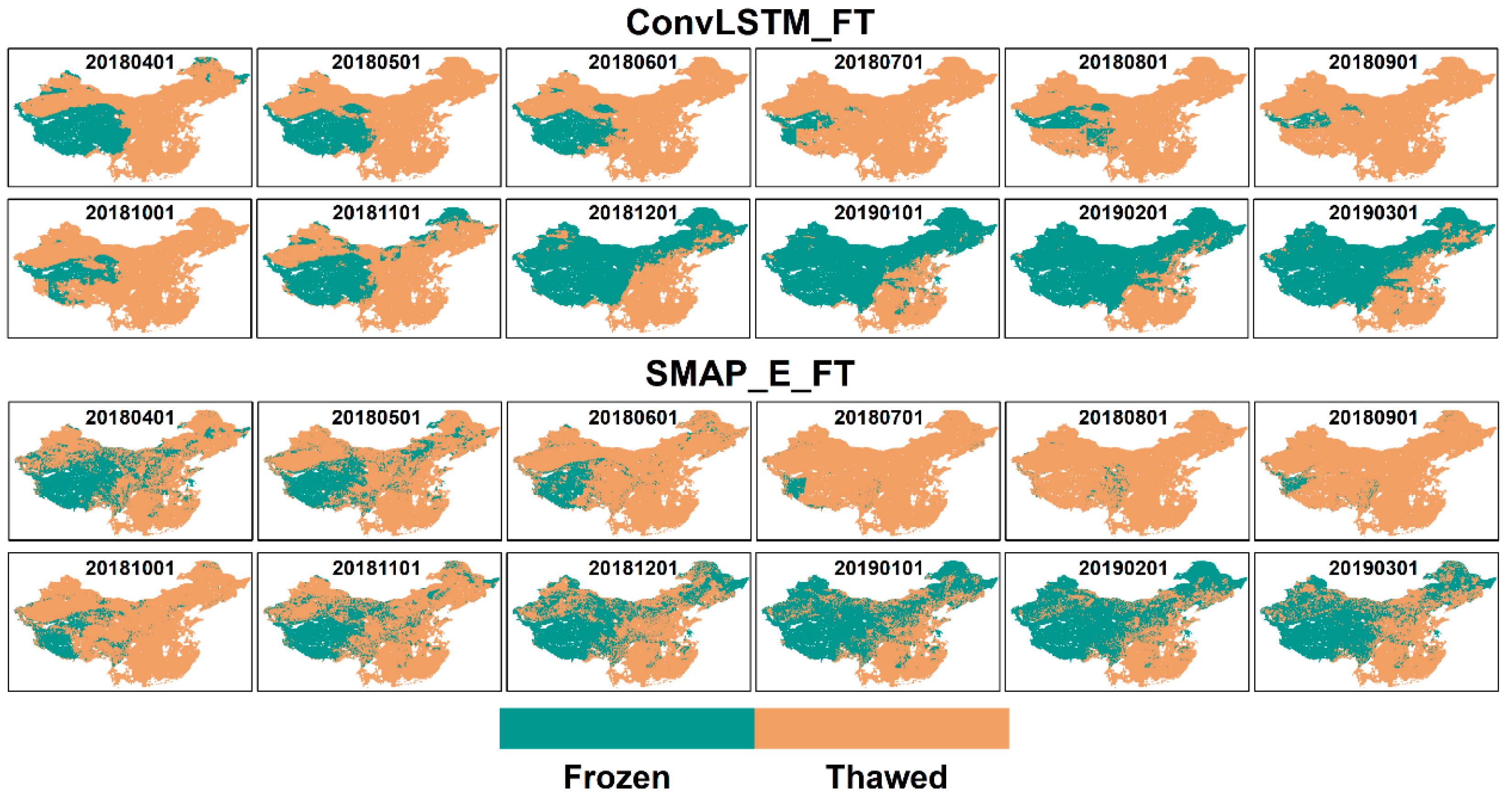
Figure 3 shows the temporal and spatial distribution of CovLSTM_FT over China throughout a whole year on every first day of each month from April 2018 to March 2019, along with the corresponding SMAP_E_FT for comparison. The variation of the frozen ground area shows a good seasonal trend, with the percentage of the frozen ground area decreasing to a minimum in summer (July, August, and September) and then gradually increasing to a maximum in winter (January). Moreover, compared with the slightly fragmented distribution of SMAP_E_FT, ConvLSTM_FT shows reasonably continuous distributions of frozen and thawed ground, which can be attributed to the introduction of ESDR_FT.
4.2. Direct Validation
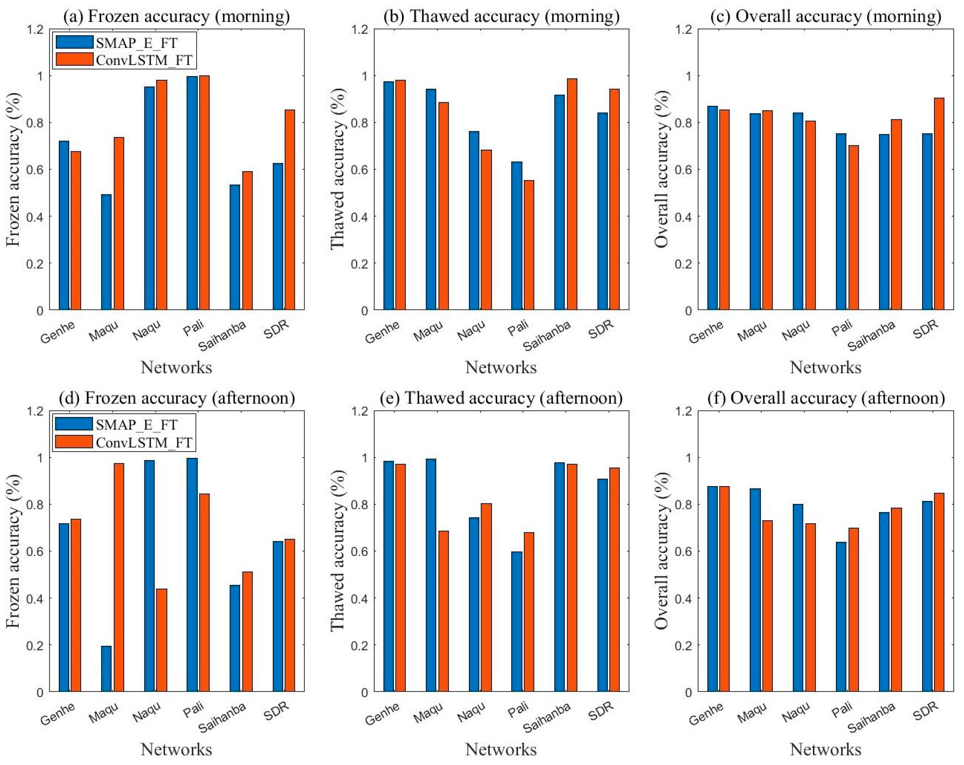
As a temporal expanding product of SMAP_E_FT, the classification accuracy of ConvLSTM_FT is very important in terms of consistency with or even superiority to that of SMAP_E_FT. In Figure 4, comparisons between frozen, thawed, and overall classification accuracies of ConvLSTM_FT and SMAP_E_FT during the test period, i.e., 1 April 2018 to 31 December 2020, are presented at the in situ networks of Genhe, Maqu, Naqu, Pali, Saihanba, and SDR. For the morning products, ConvLSTM_FT performed slightly better than SMAP_E_FT. As shown in Figure 4a, the frozen classification accuracy of ConvLSTM_FT is better than that of SMAP_E_FT at five dense in situ networks, namely Maqu, Naqu, Pali, Saihanba, and SDR, with a maximum of 0.9987 at Pali. As shown in Figure 4b, the thawed classification accuracy of ConvLSTM_FT is better than that of SMAP_E_FT at three networks, namely Genhe, Saihanba, and SDR, with a maximum of 0.9878 at Saihanba. As shown in Figure 4c, the overall classification accuracy of ConvLSTM_FT is also better than that of SMAP_E_FT at three networks, namely Maqu, Saihanba, and SDR, with a maximum of 0.9045 at SDR. Overall, ConvLSTM_FT outperforms SMAP_E_FT at 5, 3, and 3 out of 6 in situ networks regarding frozen, thawed, and overall classification accuracy. At other dense in situ networks, the classification accuracy of ConvLSTM_FT is close to that of SMAP_E_FT. For the afternoon products, it is the same situation. ConvLSTM_FT outperforms SMAP_E_FT at 4, 3, and 4 out of 6 in situ networks regarding frozen, thawed, and overall classification accuracy.
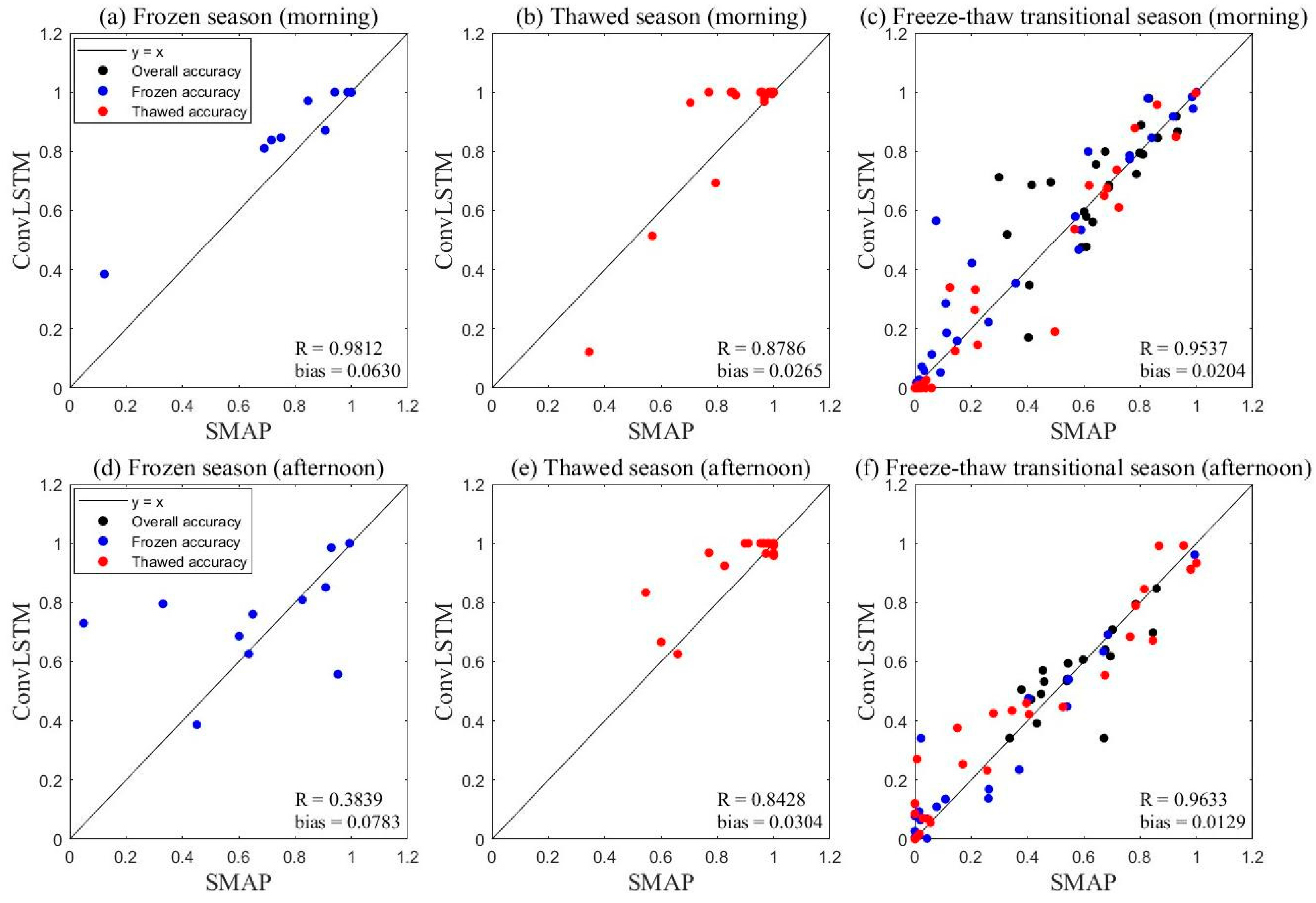
For a more comprehensive comparison of ConvLST_FT with SMAP_E_FT, we take one step further to figure out their classification performances within different seasons, i.e., the frozen, thawed, and freeze-thaw transitional seasons. According to the measurements of the six in situ networks, we divide a year into frozen season (December and January), freeze-thaw transitional season (February, March, April, October, and November), and thawed season (May, June, July, August, and September). Because there is very little thawed soil in a frozen season, comparisons between thawed classification accuracies are not included in Figure 5a,d. It is the same in Figure 5b,d that the frozen classification accuracies are not considered in a thawed season. Overall, the high correlation coefficients R between the two products indicate that ConvLSTM_FT maintains the classification accuracy of SMAP_E_FT, while the positive biases indicate that ConvLSTM_FT has a comparably higher classification accuracy at frozen, thawed, and freeze-thaw transitional seasons than SMAP_E_FT. According to the biases of morning and afternoon products in the three seasons, the superiority of ConvLSTM_FT is most significant in the frozen season, followed by the thawed and freeze-thaw transitional season. It is worth noting that, in the frozen season, the bias of 0.0630 in the morning and 0.0783 in the afternoon implies that the classification accuracy has been increased by about 7.03% relative to SMAP_FT.
4.3. Indirect Validation
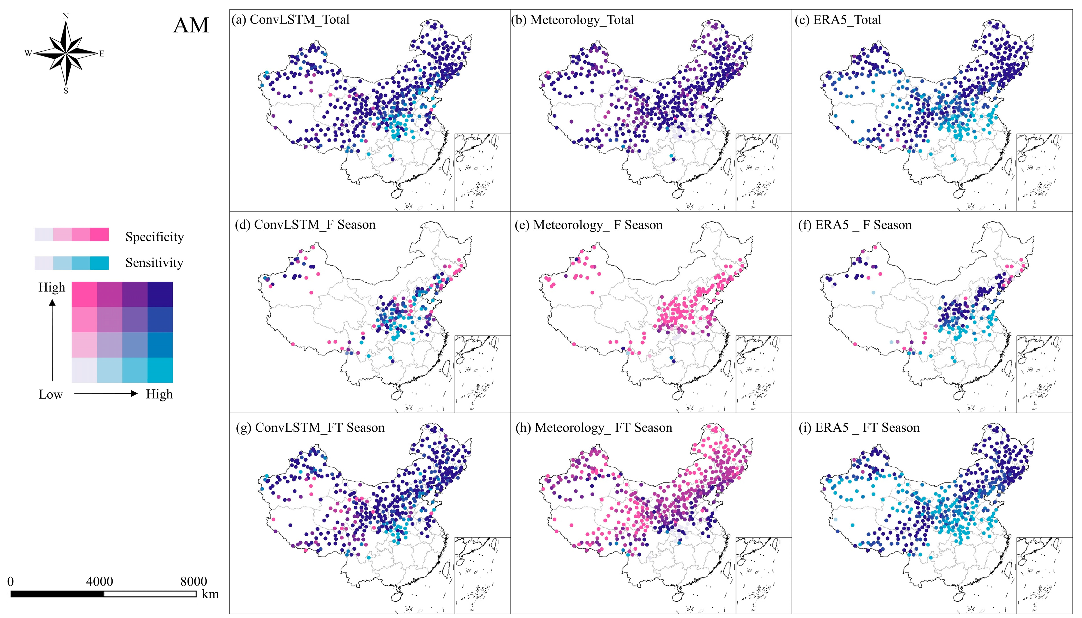
Li et al. state that long-series data can ensure a comparably reliable quantitative result from CTC [32]. In this work, the indirect validation results derived from CTC based on 41-year ConvLSTM_FT (1980–2020) are presented using a bivariate map in Figure 6 (for morning products) and Figure 7 (for afternoon products). It is worth noting that, in the thawed season, most areas in China are discriminated as thawed soil by all three products, i.e., ConvLSTM_FT, Meteorology_FT, and ERA5_FT, which violates CTC’s prerequisite of a 0-variance. Applying CTC to calculate the classification accuracies of the three FT products during the thawed season in these areas is impossible. Therefore, in Figure 6 and Figure 7, the spatial distributions of the bivariate classification accuracy for the three products are only presented by using all data, data during the frozen season, and data during the freeze-thaw transitional season.
Generally, for both morning and afternoon products, the ConvLSTM_FT has a higher frozen (sensitivity) and thawed (specificity) classification accuracy than Meteorology_FT and ERA5_FT, and overall, the frozen and thawed classification accuracies in the morning are higher than those in the afternoon. Specifically, in the morning, as shown in Figure 6, compared with ConvLSTM_FT, Meteorology_FT tends to have a lower frozen classification accuracy, while ERA5_FT tends to have a lower thawed classification accuracy, which is especially significant during the frozen and freeze-thaw transitional season. This phenomenon may be related to the fact that ERA5_FT is obtained using the soil temperature at a certain depth (0–7 cm), and Meteorology_FT is derived using a 0 cm soil temperature. In the frozen and freeze-thaw transitional seasons, the warming process in the morning (e.g., 6:00) will cause a faster increase in surface soil temperature than at a certain depth. The frozen soil at the 0 cm surface is more likely to be misclassified as thawed than soils at a certain depth, decreasing the Meteorology_FT’s frozen classification accuracy and the ERA5_FT’s thawed classification accuracy. In contrast, in the afternoon, as shown in Figure 7, compared with ConvLSTM_FT, Meteorology_FT tends to have a lower thawed classification accuracy, while ERA5_FT tends to have a lower frozen classification accuracy. Similarly, in the frozen and freeze-thaw transitional seasons, the cooling process in the afternoon (e.g., 18:00) will cause a faster decrease in surface soil temperature than at a certain depth. The thawed soil at the 0 cm surface is more likely to be misclassified as frozen than soils at a certain depth, decreasing the Meteorology_FT’s thawed classification accuracy and the ERA5_FT’s frozen classification accuracy.
5. Discussion
5.1. Analysis of ConvLSTM_FT’s Performances Based on CTC-Derived Result
In order to discuss the performances of ConvLSTM_FT from 1980 to 2020 in detail, its CTC-derived classification accuracies are further discussed and analyzed. The statistical result of ConvLSTM_FT’s frozen and thawed classification accuracies on different land cover types, Köppen climate types, and terrain complexity are presented in Figure 8, Figure 9, and Figure 10, respectively. Statistical results on ERA5_FT and Meteorology_FT are presented side-by-side for convenience of comparisons. Overall, ConvLSTM_FT maintains a stable 2nd rank in either frozen or thawed classification accuracy among the three FT products regardless of land cover types, climate types, and terrain complexity. As demonstrated and explained in the indirect validation Section 4.3, ERA5_FT performs worst when classifying thawed soils in the morning and frozen soils in the afternoon, while Meteorology_FT performs worst when classifying frozen soils in the morning and thawed soils in the afternoon. In addition, ConvLSTM_FT’s frozen classification accuracy is basically in line with the first-place product, i.e., ERA5_FT in the morning and Meteorology_FT in the afternoon, and is much better than its thawed classification accuracy. The reasons are twofold. One may be the introduction of ESDR_FT, which is better at classifying frozen soils than thawed soils [32]; the other may be L-band has better similarity between canopy and soil temperatures in the morning than in the afternoon, which will minimize the influence from vegetation [71]. In addition, the soil FT transition temperature may be affected by a variety of factors, but Meteorology_FT here is divided by 0 °C as a threshold, which may cause errors. However, due to the large number of sampling stations and large-scale study, these errors can be ignored.
China’s land cover types are mainly divided into cropland, forest, grassland, barren, and impervious [65], as shown in Figure 8. Regarding frozen classification accuracy, ConvLSTM_FT performs very well with an average sensitivity , i.e., the frozen classification accuracy, of 0.96 and 0.98 in the morning and afternoon, respectively, as shown in Figure 8a,c, which indicates that, as a temporal expanding product of SMAP_E_FT, ConvLSTM_FT well inherits L-band’s sensitivity to transient changes of soil FT state in the frozen season [72]. Studies have shown that in many land cover types, even in forests, the L-band is highly likely to be affected by surface temperature reduction to capture more frozen signals in the early frozen stage [26,73]. However, the performance of ConvLSTM_FT is also affected by the different penetration abilities of the L-band to different vegetation. It can be observed clearly from Figure 8b,d that ConvLSTM performs the best in barren areas but the worst in forests. The same phenomenon also appears in SMAP_E_FT. That is, the classification accuracy will decrease as the vegetation becomes dense [36].
According to the Köppen climate classification data [66], there are four different climate types in China: arid, temperate, continental, and polar. Regarding frozen classification accuracy, as shown in Figure 9a,c, ConvLSTM_FT performed very well (both above 0.96 in the morning and afternoon). However, the performance in polar areas is slightly worse than that of other regions, which may be due to the fact that when the temperature rises above zero in early spring, the presence of wet snow on the surface of frozen soil will lead to the increase of dielectric constant and thus misjudged as thawed state [26,73,74,75]. Interestingly, ConvLSTM_FT performs best in polar areas and worst in temperate areas when classifying thawed soils, as shown in Figure 9b,d. That may be due to the greater uncertainty in the classification of FT in areas where FT transitions are frequent (e.g., the temperate area), which echoes the demonstration of Chai et al. that the classification accuracy in an FT transitional season is lower than in a frozen or thawed season [31].
The terrain complexity is evaluated using TCI. Figure 10 shows the statistical result of ConvLSTM_FT’s frozen and thawed classification accuracy on different TCI conditions, divided into less than 50 m, 50 to 150 m, 150 to 250 m, 250 to 350 m, and no less than 350 m. As shown in Figure 10a,c, ConvLSTM_FT performs very well (above 0.9 and 0.97 in the morning and afternoon, respectively). Generally, ConvLSTM_FT’s classification accuracy has a decreasing trend with an increased TCI, corresponding to an increased terrain complexity. This may be because more frequent FT processes are more likely to occur in mountainous regions with higher elevations, making it more challenging to capture FT signals accurately [5,76]. As a result, with the increase in TCI, the classification accuracy will decrease [29,74].
5.2. Soil Freeze/Thaw Trend in the ConvLSTM_FT over 1980–2020
Based on ConvLSTM_FT’s 9 km soil FT products in China from 1980 to 2020, frozen days in those years are counted year by year within China’s four regions: Qinghai–Tibet, northwest, north, and south. Based on the trend analysis method, Figure 11 presents the variation of the average number of frozen days in each region from 1980 to 2020, with the southern region excluded because there are generally only thawed soils all year around in southern China. The results show that, from 1980 to 2020, the number of frozen days in the three regions averaged 168 days, with an average decreasing trend of −0.21 d/a. As expected, the Qinghai–Tibet region owns the longest frozen days, with a mean value of 239 days, followed by the northwestern and northern regions, with a mean value of 144 days and 102 days, respectively. Although all three regions have experienced a decreasing trend in the number of frozen days, they are different from each other. Specifically, as shown in Figure 11 and Table 2, the decreasing rate is the fastest in the northwest, while the average frozen days decreased the slowest in Qinghai–Tibet. The phenomenon may be directly related to the global warming. We know that more areas in the northern and northwestern regions are seasonally frozen ground (SFG) than the Qinghai–Tibet region (with more permafrost areas). Studies have shown that the impact of increasing air temperature on the variations of frozen days will be more direct and significant in SFG than in permafrost [77]. That is probably because SFG is located at the top layer of the ground, while the long-term degradation process of permafrost has a resistant effect to more frequent FT transitions caused by increased temperature [78].
We further analyze and discuss the decreasing rate of frozen days in the past 41 years (1980–2020) within Qinghai–Tibet under the subcategories of permafrost, which is divided by Ran et al. based on the thermal stability of permafrost [67]. The thermal stability of the permafrost is evaluated according to the mean annual ground temperature and ranked from high to low as very stable, stable, semi-stable, transitional, and unstable. It can be observed from Figure 12 that, from 1980 to 2020, the variation trends in the average number of frozen days decreased across all six frozen grounds under different thermal stabilities. The decreasing rate of frozen days gradually slows down as thermal stability decreases, with very stable of −0.31 d/a, stable of −0.22 d/a, semi-stable of −0.11 d/a, transitional of −0.09 d/a, and unstable of −0.05 d/a (Table 2).
In the context of global warming, permafrost degradation will generally go through five processes: starting stage, temperature rising stage, zero gradient stage, talic layers stage, and disappearing stage [79]. In a temperature rising stage, ground temperature increases rapidly, permafrost degrades violently [80], and thawed interlayers appear in the permafrost with the rapid temperature rise. In addition, because there is a perennially high temperate zone near the upper limit of permafrost, thawing will be accelerated under the effect of “anti-seasonal compensation” [79]. In zero gradient, disjointed, and disappearing stages, the increasing rate of ground temperature gradually slows down, inducing the permafrost degradation rate to slow down, with the permafrost thawing from the top and disappearing eventually. According to space-time substitution, the rise of permafrost’s thermal stability may be reasonably linked to permafrost degradation. Studies have shown that under the current warming conditions, the degradation of very stable or stable permafrost in the Qinghai–Tibet region may be in the starting and temperature rising stages [81]. This also explains the gradual inclination in the decreasing rate of frozen days as the thermal stability increases.

| Region | SFG | Permafrost | Slope (d/a) | |
|---|---|---|---|---|
| Area Percent | Thermal Stability | Area Percent | ||
| Northwest | 43.04% | / | 56.96% | −0.32 |
| North | 97.00% | / | 2.00% | −0.29 |
| Qinghai–Tibet | 41.60% | / | 47.92% | −0.06 |
| Within Qinghai–Tibet | / | Very stable | 0.36% | −0.31 |
| Stable | 4.01% | −0.22 | ||
| Semi-stable | 16.02% | −0.11 | ||
| Transitional | 17.62% | −0.09 | ||
| Unstable | 9.92% | −0.05 | ||
| 41.60% | / | / | −0.02 | |
6. Conclusions
In this work, a 41-year ConvLSTM_FT product (1980–2020) was generated by expanding the time series of SMAP_FT products based on the Convolutional Long Short-Term Memory model. The classification accuracies of ConvLSTM for frozen and thawed soils are directly validated based on six dense in situ networks and indirectly validated using CTC by constructing a triplet together with ERA5_FT and Meteorology_FT. Moreover, the variation trends in soil frozen days during the past 41 years over three major geographical regions within China and different thermal stabilities of frozen ground within Qinghai–Tibet are analyzed based on ConvLSTM_FT. Three key conclusions are obtained.
- (1)
- The ConvLSTM model can capture spatiotemporal information effectively, and the introduction of decision-level fusion can further improve the prediction accuracy of ConvLSTM. Therefore, the decision-level spatiotemporal fusion architecture based on the ConvLSTM model is an effective method worth trying in the research of data fusion, time series extension, and classification accuracy improvement.
- (2)
- As a temporal expanding product of SMAP_E_FT, ConvLSTM_FT overall outperforms SMAP_E_FT. Direct verification results show that the overall classification accuracy of ConvLSTM_FT has an improvement of 2.44% relative to SMAP_E_FT, especially in frozen seasons (improved by an average of 7.03%). Indirect verification results show that ConvLSTM_FT is more stable than ERA5_FT and Meterology_FT, ranking second in the accuracy of FT soil identification regardless of land cover types, climate types, and terrain complexity.
- (3)
- The analysis result of the classification accuracy of ConvLSTM_FT from 1980 to 2020 shows that the annual frozen days and their changes are reasonable in the northwest, north, and Qinghai–Tibet regions of China. Especially in the Qinghai–Tibet region, with the decrease in permafrost thermal stability, the rate of frozen soil degradation slows down. These results are reasonable and can effectively reflect the impact of climate change on frozen soils in the past 41 years.
In future research, we aim to address the limitations identified in this study. Because of the limitation of ground observation technology, it is still currently difficult to accurately determine the specific temperature of FT transition on a large scale. We will create a more reliable ground truth dataset from measured data for validation purposes.
Author Contributions
Conceptualization, L.C., H.L. and H.C.; methodology and software, H.L.; validation, H.C.; formal analysis, H.C. and H.L.; investigation, H.L. and H.C.; resources, L.C., S.Z. and S.L.; data curation, L.C.; writing—original draft preparation, H.C. and H.L.; writing—review and editing, L.C.; visualization, H.C. and H.L.; supervision, project administration and funding acquisition, L.C. and X.L. All authors have read and agreed to the published version of the manuscript.
Funding
This research was funded by the Second Tibetan Plateau Scientific Expedition and Research Program (STEP) (2019QZKK0306) and the National Natural Science Foundation of China (42171319).
Data Availability Statement
The datasets presented in this paper is available through https://doi.org/10.11888/Terre.tpdc.300469.
Conflicts of Interest
The authors declare no conflicts of interest.
References
- Zhang, T.; Armstrong, R.L.; Smith, J. Investigation of the near-surface soil freeze-thaw cycle in the contiguous United States: Algorithm development and validation. J. Geophys. Res. Atmos. 2003, 108, 8860. [Google Scholar] [CrossRef]
- Zhang, T.J.; Barry, R.; Armstrong, R. Application of Satellite Remote Sensing Techniques to Frozen Ground Studies. Polar Geogr. 2004, 28, 24–55. [Google Scholar] [CrossRef]
- Nelson, F.E.; Anisimov, O.A.; Shiklomanov, N.I. Climate change and hazard zonation in the circum-Arctic permafrost regions. Nat. Hazards 2002, 26, 203–225. [Google Scholar] [CrossRef]
- Jin, R.; Zhang, T.; Li, X.; Yang, X.; Ran, Y. Mapping surface soil freeze-thaw cycles in China based on SMMR and SSM/I brightness temperatures from 1978 to 2008. Arct. Antarct. Alp. Res 2015, 47, 213–229. [Google Scholar] [CrossRef]
- Johnston, J.; Maggioni, V.; Houser, P. Comparing global passive microwave freeze/thaw records: Investigating differences between Ka- and L-band products. Remote Sens. Environ. 2020, 247, 111936. [Google Scholar] [CrossRef]
- Wang, J.; Jiang, L.; Cui, H.; Wang, G.; Yang, J.; Liu, X.; Su, X. Evaluation and analysis of SMAP, AMSR2 and MEaSUREs freeze/thaw products in China. Remote Sens. Environ. 2020, 242, 111734. [Google Scholar] [CrossRef]
- Schuur, E.A.G.; McGuire, A.D.; Schädel, C.; Grosse, G.; Harden, J.W.; Hayes, D.J.; Hugelius, G.; Koven, C.D.; Kuhry, P.; Lawrence, D.M.; et al. Climate change and the permafrost carbon feedback. Nature 2015, 520, 171–179. [Google Scholar] [CrossRef] [PubMed]
- Peng, X.; Frauenfeld, O.W.; Cao, B.; Wang, K.; Wang, H.; Su, H.; Huang, Z.; Yue, D.; Zhang, T. Response of changes in seasonal soil freeze/thaw state to climate change from 1950 to 2010 across China. J. Geophys. Res. Earth Surf. 2016, 121, 1984–2000. [Google Scholar] [CrossRef]
- Mu, C.; Zhang, T.; Wu, Q.; Peng, X.; Cao, B.; Zhang, X.; Cao, B.; Cheng, G. Editorial: Organic carbon pools in permafrost regions on the Qinghai-Xizang (Tibetan) Plateau. Cryosphere 2015, 9, 479–486. [Google Scholar] [CrossRef]
- Tarnocai, C.; Canadell, J.G.; Schuur, E.A.G.; Kuhry, P.; Mazhitova, G.; Zimov, S. Soil organic carbon pools in the northern circumpolar permafrost region. Glob. Biogeochem. Cycles 2009, 23, GB2023. [Google Scholar] [CrossRef]
- Philipp, M.; Dietz, A.; Buchelt, S.; Kuenzer, C. Trends in Satellite Earth Observation for Permafrost Related Analyses—A Review. Remote Sens. 2021, 13, 1217. [Google Scholar] [CrossRef]
- Qin, S.; Kou, D.; Mao, C.; Chen, Y.; Chen, L.; Yang, Y. Temperature sensitivity of permafrost carbon release mediated by mineral and microbial properties. Sci. Adv. 2021, 7, eabe3596. [Google Scholar] [CrossRef] [PubMed]
- Cao, W.; Cao, Y.; Sheng, Y.; Chou, Y.; Wu, J.; Peng, E. The evolution process and degradation model of permafrost in the Source Area of the Yellow River on the Qinghai-Tibet Plateau since the Little Ice Age. Catena 2024, 236, 107671. [Google Scholar] [CrossRef]
- Deng, H.; Zhang, Z.; Wu, Y. Accelerated permafrost degradation in thermokarst landforms in Qilian Mountains from 2007 to 2020 observed by SBAS-InSAR. Ecol. Indic. 2024, 159, 111724. [Google Scholar] [CrossRef]
- Sun, Z.; Ma, W.; Li, G.; Liu, Y.; Wu, G. Degrading permafrost beneath road embankments of the Qinghai-Tibet Highway from 1995 to 2020. Cold Reg. Sci. Technol. 2024, 219, 104133. [Google Scholar] [CrossRef]
- Ye, C.; Wang, S.; Wu, S.; Zhou, T. Impacts of future permafrost degradation and human modification on terrestrial vertebrates. Biol. Conserv. 2024, 291, 110475. [Google Scholar] [CrossRef]
- Che, L.; Zhang, H.; Wan, L. Spatial distribution of permafrost degradation and its impact on vegetation phenology from 2000 to 2020. Sci. Total Environ. 2023, 877, 162889. [Google Scholar] [CrossRef] [PubMed]
- Tananaev, N.; Lotsari, E. Defrosting northern catchments: Fluvial effects of permafrost degradation. Earth-Sci. Rev. 2022, 228, 103996. [Google Scholar] [CrossRef]
- Xin, L. China Long-Sequence Surface Freeze-Thaw Dataset—Decision Tree Algorithm (1987–2009). A Big Earth Data Platform for Three Poles. 2012. Available online: http://60.245.210.47/en/data/c5f2a6bd-f481-4390-851f-3519d6eb7fdd/ (accessed on 30 June 2023).
- Zuerndorfer, B.; England, A.W. Radiobrightness Decision Criteria for Freeze Thaw Boundaries. IEEE Trans. Geosci. Remote Sens. 1992, 30, 89–102. [Google Scholar] [CrossRef]
- Judge, J.; Galantowicz, J.F.; England, A.W.; Dahl, P. Freeze/thaw classification for prairie soils using SSM/I radiobrightnesses. IEEE Trans. Geosci. Remote Sens. 1997, 35, 827–832. [Google Scholar] [CrossRef]
- Xin, L. Long-Term Surface Soil Freeze-Thaw States Dataset of China Using the Dual-Index Algorithm (1978–2015). A Big Earth Data Platform for Three Poles. 2011. Available online: http://60.245.210.47/en/data/76bce7bb-e1b2-49c4-9537-668a6bac42a2/ (accessed on 30 June 2023).
- Tianjie, Z. 2002–2019 Global AMSR-E/2 Near-Surface Freeze/Thaw State (0.25°). A Big Earth Data Platform for Three Poles. 2018. Available online: http://60.245.210.47/en/data/d1b437cb-10b9-496c-96b4-76e3d185dd47/ (accessed on 30 June 2023).
- Kim, Y.; Kimball, J.S.; McDonald, K.C.; Glassy, J. Developing a Global Data Record of Daily Landscape Freeze/Thaw Status Using Satellite Passive Microwave Remote Sensing. IEEE Trans. Geosci. Remote Sens. 2011, 49, 949–960. [Google Scholar] [CrossRef]
- Kim, S.; Arii, M.; Jackson, T. Modeling L-Band Synthetic Aperture Radar Data Through Dielectric Changes in Soil Moisture and Vegetation Over Shrublands. IEEE J. Sel. Top. Appl. Earth Observ. Remote Sens. 2017, 10, 4753–4762. [Google Scholar] [CrossRef]
- Rautiainen, K.; Lemmetyinen, J.; Schwank, M.; Kontu, A.; Ménard, C.B.; Mätzler, C.; Drusch, M.; Wiesmann, A.; Ikonen, J.; Pulliainen, J. Detection of soil freezing from L-band passive microwave observations. Remote Sens. Environ. 2014, 147, 206–218. [Google Scholar] [CrossRef]
- Derksen, C.; Xu, X.; Dunbar, R.S.; Colliander, A.; Kim, Y.; Kimball, J.S.; Black, T.A.; Euskirchen, E.; Langlois, A.; Loranty, M.M.; et al. Retrieving landscape freeze/thaw state from Soil Moisture Active Passive (SMAP) radar and radiometer measurements. Remote Sens. Environ. 2017, 194, 48–62. [Google Scholar] [CrossRef]
- Rautiainen, K.; Parkkinen, T.; Lemmetyinen, J.; Schwank, M.; Wiesmann, A.; Ikonen, J.; Derksen, C.; Davydov, S.; Davydova, A.; Boike, J.; et al. SMOS prototype algorithm for detecting autumn soil freezing. Remote Sens. Environ. 2016, 180, 346–360. [Google Scholar] [CrossRef]
- Chai, L.; Zhang, L.; Zhang, Y.; Hao, Z.; Jiang, L.; Zhao, S. Comparison of the classification accuracy of three soil freeze—Thaw discrimination algorithms in China using SSMIS and AMSR-E passive microwave imagery. Int. J. Remote Sens. 2014, 35, 7631–7649. [Google Scholar] [CrossRef]
- Shao, W.; Zhang, T. Assessment of Four Near- Surface Soil Freeze/Thaw Detection Algorithms Based on Calibrated Passive Microwave Remote Sensing Data Over China. Earth Space Sci. 2020, 7, e2019EA000807. [Google Scholar] [CrossRef]
- Chai, L.; Zhu, Z.; Liu, S.; Xu, Z.; Jin, R.; Li, X.; Kang, J.; Che, T.; Zhang, Y.; Zhang, J.; et al. QLB-NET: A Dense Soil Moisture and Freeze/Thaw Monitoring Network in the Qinghai Lake Basin on the Qinghai-Tibetan Plateau. Bull. Am. Meteorol. Soc. 2023, in press. [Google Scholar] [CrossRef]
- Li, H.; Chai, L.; Crow, W.; Dong, J.; Liu, S.; Zhao, S. The reliability of categorical triple collocation for evaluating soil freeze/thaw datasets. Remote Sens. Environ. 2022, 281, 113240. [Google Scholar] [CrossRef]
- Zheng, J.; Zhao, T.; Lü, H.; Zou, D.; Rodriguez-Fernandez, N.; Mialon, A.; Richaume, P.; Xiao, J.; Ma, J.; Fan, L.; et al. Use of a new Tibetan Plateau network for permafrost to characterize satellite-based products errors: An application to soil moisture and freeze/thaw. Remote Sens. Environ. 2024, 300, 113899. [Google Scholar] [CrossRef]
- Zhao, T.; Zhang, L.; Jiang, L.; Zhao, S.; Chai, L.; Jin, R. A new soil freeze/thaw discriminant algorithm using AMSR-E passive microwave imagery. Hydrol. Process 2011, 25, 1704–1716. [Google Scholar] [CrossRef]
- Smith, N.V.; Saatchi, S.S.; Randerson, J.T. Trends in high northern latitude soil freeze and thaw cycles from 1988 to 2002. J. Geophys. Res. Atmos. 2004, 109, D12101. [Google Scholar] [CrossRef]
- Xu, X.; Dunbar, R.S.; Derksen, C.; Colliander, A.; Kim, Y.; Kimball, J.S. SMAP Enhanced L3 Radiometer Global and Polar Grid Daily 9 km EASE-Grid Soil Moisture; Version 5; NASA National Snow and Ice Data Center Distributed Active Archive Center: Boulder, CO, USA, 2020; Volume 2023. [Google Scholar]
- Xu, X.; Dunbar, R.S.; Derksen, C.; Colliander, A.; Kim, Y.; Kimball, J.S. SMAP L3 Radiometer Global and Northern Hemisphere Daily 36 km EASE-Grid Freeze/Thaw State; Version 3; NASA National Snow and Ice Data Center Distributed Active Archive Center: Boulder, CO, USA, 2020; Volume 2023. [Google Scholar]
- Chen, X.; Jeong, S.; Park, C.; Park, H.; Joo, J.; Chang, D.; Yun, J. Different responses of surface freeze and thaw phenology changes to warming among Arctic permafrost types. Remote Sens. Environ. 2022, 272, 112956. [Google Scholar] [CrossRef]
- Lecun, Y.; Bengio, Y. Convolutional Networks for Images, Speech, and Time-Series. In The Handbook of Brain Theory and Neural Networks; MIT Press: Cambridge, MA, USA, 1995. [Google Scholar]
- Hochreiter, S.; Schmidhuber, J. Long short-term memory. Neural Comput. 1997, 9, 1735–1780. [Google Scholar] [CrossRef] [PubMed]
- Shi, X.; Chen, Z.; Wang, H.; Yeung, D.; Wong, W.; Woo, W. Convolutional LSTM Network: A Machine Learning Approach for Precipitation Nowcasting. In Advances in Neural Information Processing Systems 28 (Nips 2015); North Torrey Pines Rd: La Jolla, CA, USA, 2015; Volume 28. [Google Scholar]
- Tan, J.; NourEldeen, N.; Mao, K.; Shi, J.; Li, Z.; Xu, T.; Yuan, Z. Deep Learning Convolutional Neural Network for the Retrieval of Land Surface Temperature from AMSR2 Data in China. Sensors 2019, 19, 2987. [Google Scholar] [CrossRef] [PubMed]
- Dong, J.; Zhu, Y.; Jia, X.; Shao, M.; Han, X.; Qiao, J.; Bai, C.; Tang, X. Nation-scale reference evapotranspiration estimation by using deep learning and classical machine learning models in China. J. Hydrol. 2022, 604, 127207. [Google Scholar] [CrossRef]
- Sobayo, R.; Wu, H.; Ray, R.L.; Qian, L. Integration of Convolutional Neural Network and Thermal Images into Soil Moisture Estimation. In Proceedings of the 2018 1St International Conference on Data Intelligence and Security (ICDIS 2018), South Padre Island, TX, USA, 8–10 April 2018; pp. 207–210. [Google Scholar]
- Pan, B.; Hsu, K.; AghaKouchak, A.; Sorooshian, S. Improving Precipitation Estimation Using Convolutional Neural Network. Water Resour. Res. 2019, 55, 2301–2321. [Google Scholar] [CrossRef]
- Fang, K.; Shen, C. Near-Real-Time Forecast of Satellite-Based Soil Moisture Using Long Short-Term Memory with an Adaptive Data Integration Kernel. J. Hydrometeorol. 2020, 21, 399–413. [Google Scholar] [CrossRef]
- Li, Q.; Zhao, Y.; Yu, F. A Novel Multichannel Long Short-Term Memory Method with Time Series for Soil Temperature Modeling. IEEE Access 2020, 8, 182026–182043. [Google Scholar] [CrossRef]
- Wang, H.; Zhao, X.; Zhang, X.; Wu, D.; Du, X. Long Time Series Land Cover Classification in China from 1982 to 2015 Based on Bi-LSTM Deep Learning. Remote Sens 2019, 11, 1639. [Google Scholar] [CrossRef]
- Chen, Z.; Zhu, Z.; Jiang, H.; Sun, S. Estimating daily reference evapotranspiration based on limited meteorological data using deep learning and classical machine learning methods. J. Hydrol. 2020, 591, 125286. [Google Scholar] [CrossRef]
- Wu, H.; Yang, Q.; Liu, J.; Wang, G. A spatiotemporal deep fusion model for merging satellite and gauge precipitation in China. J. Hydrol. 2020, 584, 124664. [Google Scholar] [CrossRef]
- Munoz-Sabater, J.; Dutra, E.; Agusti-Panareda, A.; Albergel, C.; Arduini, G.; Balsamo, G.; Boussetta, S.; Choulga, M.; Harrigan, S.; Hersbach, H.; et al. ERA5-Land: A state-of-the-art global reanalysis dataset for land applications. Earth Syst. Sci. Data 2021, 13, 4349–4383. [Google Scholar] [CrossRef]
- Xu, X.; Wang, J.; Zhang, L. Physics of Frozen Soil; Science Press: Beijing, China, 2001. [Google Scholar]
- Li, X.; Cheng, G.; Jin, H.; Kang, E.; Che, T.; Jin, R.; Wu, L.; Nan, Z.; Wang, J.; Shen, Y. Cryospheric change in China. Glob. Planet. Change 2008, 62, 210–218. [Google Scholar] [CrossRef]
- Jiang, L.; Wang, J.; Cui, H.; Wang, G.; Zhao, T.; Zhao, S.; Chai, L.; Liu, X.; Yang, J. In situ soil moisture and temperature network in genhe watershed and saihanba area in China. Data Brief. 2020, 31, 105693. [Google Scholar] [CrossRef] [PubMed]
- Yang, K.; Qin, J.; Zhao, L.; Chen, Y.; Tang, W.; Han, M.; Chen, Z.; Lv, N.; Ding, B.; Wu, H.; et al. A Multiscale Soil Moisture and Freeze–Thaw Monitoring Network on the Third Pole. Bull. Am. Meteorol. Soc. 2013, 94, 1907–1916. [Google Scholar] [CrossRef]
- Su, Z.; Wen, J.; Dente, L.; van der Velde, R.; Wang, L.; Ma, Y.; Yang, K.; Hu, Z. The Tibetan Plateau observatory of plateau scale soil moisture and soil temperature (Tibet-Obs) for quantifying uncertainties in coarse resolution satellite and model products. Hydrol. Earth Syst. Sci. 2011, 15, 2303–2316. [Google Scholar] [CrossRef]
- Zhao, T.; Shi, J.; Lv, L.; Xu, H.; Chen, D.; Cui, Q.; Jackson, T.J.; Yan, G.; Jia, L.; Chen, L.; et al. Soil moisture experiment in the Luan River supporting new satellite mission opportunities. Remote Sens. Environ. 2020, 240, 111680. [Google Scholar] [CrossRef]
- Wen, Y.; Liu, B.; Jiang, H.; Li, T.; Zhang, B.; Wu, W. Initial soil moisture prewinter affects the freeze–thaw profile dynamics of a Mollisol in Northeast China. Catena 2024, 234, 107648. [Google Scholar] [CrossRef]
- Agency, X.N. The People’s Republic of China Yearbook; Xinhua Publishing House: Beijing, China, 2021. [Google Scholar]
- Kim, Y.; Kimball, J.S.; Glassy, J.; Du, J. An extended global Earth system data record on daily landscape freeze—Thaw status determined from satellite passive microwave remote sensing. Earth Syst. Sci. Data 2017, 9, 133–147. [Google Scholar] [CrossRef]
- Hersbach, H.; Bell, B.; Berrisford, P.; Hirahara, S.; Horányi, A.; Muñoz-Sabater, J.; Nicolas, J.; Peubey, C.; Radu, R.; Schepers, D.; et al. The ERA5 global reanalysis. Q. J. R. Meteorol. Soc. 2020, 146, 1999–2049. [Google Scholar] [CrossRef]
- Hou, A.Y.; Kakar, R.K.; Neeck, S.; Azarbarzin, A.A.; Kummerow, C.D.; Kojima, M.; Oki, R.; Nakamura, K.; Iguchi, T. The Global Precipitation Measurement Mission. Bull. Am. Meteorol. Soc. 2014, 95, 701. [Google Scholar] [CrossRef]
- Xu, R.; Tian, F.; Yang, L.; Hu, H.; Lu, H.; Hou, A. Ground validation of GPM IMERG and TRMM 3B42V7 rainfall products over southern Tibetan Plateau based on a high-density rain gauge network. J. Geophys. Res. Atmos. 2017, 122, 910–924. [Google Scholar] [CrossRef]
- Ma, Y.; Tang, G.; Long, D.; Yong, B.; Zhong, L.; Wan, W.; Hong, Y. Similarity and Error Intercomparison of the GPM and Its Predecessor-TRMM Multisatellite Precipitation Analysis Using the Best Available Hourly Gauge Network over the Tibetan Plateau. Remote Sens. 2016, 8, 569. [Google Scholar] [CrossRef]
- Yang, J.; Huang, X. The 30 m annual land cover dataset and its dynamics in China from 1990 to 2019. Earth Syst. Sci. Data 2021, 13, 3907–3925. [Google Scholar] [CrossRef]
- Kottek, M.; Grieser, J.; Beck, C.; Rudolf, B.; Rubel, F. World map of the Koppen-Geiger climate classification updated. Meteorol. Z. 2006, 15, 259–263. [Google Scholar] [CrossRef]
- Ran, Y.; Li, X.; Cheng, G.; Nan, Z.; Che, J.; Sheng, Y.; Wu, Q.; Jin, H.; Luo, D.; Tang, Z.; et al. Mapping the permafrost stability on the Tibetan Plateau for 2005–2015. Sci. China Earth Sci. 2021, 64, 62–79. [Google Scholar] [CrossRef]
- Moishin, M.; Deo, R.C.; Prasad, R.; Raj, N.; Abdulla, S. Designing Deep-Based Learning Flood Forecast Model with ConvLSTM Hybrid Algorithm. IEEE Access 2021, 9, 50982–50993. [Google Scholar] [CrossRef]
- McColl, K.A.; Roy, A.; Derksen, C.; Konings, A.G.; Alemohammed, S.H.; Entekhabi, D. Triple collocation for binary and categorical variables: Application to validating landscape freeze/thaw retrievals. Remote Sens. Environ. 2016, 176, 31–42. [Google Scholar] [CrossRef]
- Scott, K.A. Assessment of Categorical Triple Collocation for Sea Ice/Open Water Observations: Application to the Gulf of Saint Lawrence. IEEE Trans. Geosci. Remote Sens. 2019, 57, 9659–9673. [Google Scholar] [CrossRef]
- Entekhabi, D.; Njoku, E.G.; O’Neill, P.E.; Kellogg, K.H.; Crow, W.T.; Edelstein, W.N.; Entin, J.K.; Goodman, S.D.; Jackson, T.J.; Johnson, J.; et al. The Soil Moisture Active Passive (SMAP) Mission. Proc. IEEE 2010, 98, 704–716. [Google Scholar] [CrossRef]
- Chen, X.; Liu, L.; Bartsch, A. Detecting soil freeze/thaw onsets in Alaska using SMAP and ASCAT data. Remote Sens. Environ. 2019, 220, 59–70. [Google Scholar] [CrossRef]
- Roy, A.; Royer, A.; Derksen, C.; Brucker, L.; Langlois, A.; Mialon, A.; Kerr, Y.H. Evaluation of Spaceborne L-Band Radiometer Measurements for Terrestrial Freeze/Thaw Retrievals in Canada. IEEE J. Sel. Top. Appl. Earth Obs. Remote Sens. 2015, 8, 4442–4459. [Google Scholar] [CrossRef]
- Kim, Y.; Kimball, J.S.; Xu, X.; Dunbar, R.S.; Colliander, A.; Derksen, C. Global Assessment of the SMAP Freeze/Thaw Data Record and Regional Applications for Detecting Spring Onset and Frost Events. Remote Sens. 2019, 11, 1317. [Google Scholar] [CrossRef]
- Roy, A.; Toose, P.; Williamson, M.; Rowlandson, T.; Derksen, C.; Royer, A.; Berg, A.A.; Lemmetyinen, J.; Arnold, L. Response of L-Band brightness temperatures to freeze/thaw and snow dynamics in a prairie environment from ground-based radiometer measurements. Remote Sens. Environ. 2017, 191, 67–80. [Google Scholar] [CrossRef]
- Dunbar, S. SMAP—Algorithm Theoretical Basis Document (ATBD)—Level 3 Radiometer Freeze/Thaw Data Products; Jet Propulsion Laboratory, California Institute of Technology: Pasadena, CA, USA, 2020; Available online: https://nsidc.org/sites/default/files/l3_ft_p_atbd_revisionc_vf.pdf (accessed on 22 July 2022).
- Xu, S.; Liu, D.; Li, T.; Fu, Q.; Liu, D.; Hou, R.; Meng, F.; Li, M.; Li, Q. Spatiotemporal evolution of the maximum freezing depth of seasonally frozen ground and permafrost continuity in historical and future periods in Heilongjiang Province, China. Atmos. Res. 2022, 274, 106195. [Google Scholar] [CrossRef]
- Guo, D.; Wang, H. CMIP5 permafrost degradation projection: A comparison among different regions. J. Geophys. Res. 2016, 121, 4499–4517. [Google Scholar] [CrossRef]
- Wu, J.; Sheng, Y.; Wu, Q.; Wen, Z. Processes and modes of permafrost degradation on the Qinghai-Tibet Plateau. Sci. China Ser. D Earth Sci. 2010, 53, 150–158. [Google Scholar] [CrossRef]
- Yu, F.; Qi, J.; Yao, X.; Liu, Y. Degradation process of permafrost underneath embankments along Qinghai-Tibet Highway: An engineering view. Cold Reg. Sci. Technol. 2013, 85, 150–156. [Google Scholar] [CrossRef]
- Jin, H.; Zhao, L.; Wang, S.; Jin, R. Thermal regimes and degradation modes of permafrost along the Qinghai-Tibet Highway. Sci. China Ser. D Earth Sci. 2006, 49, 1170–1183. [Google Scholar] [CrossRef]
- Ran, Y.; Li, X.; Cheng, G.; Zhang, T.; Wu, Q.; Jin, H.; Jin, R. Distribution of Permafrost in China: An Overview of Existing Permafrost Maps. Permafr. Periglac. Process. 2012, 23, 322–333. [Google Scholar] [CrossRef]
Figure 1.
Study area and in situ observations. (a) Spatial distribution of meteorological stations and six dense in situ observation networks in China, with China’s four major geographical regions [59]. (b–g) The dense in situ soil moisture and soil temperature networks.
Figure 1.
Study area and in situ observations. (a) Spatial distribution of meteorological stations and six dense in situ observation networks in China, with China’s four major geographical regions [59]. (b–g) The dense in situ soil moisture and soil temperature networks.

Figure 2.
The architecture of a ConvLSTM and the spatiotemporal fusion algorithm structure at the decision layer based on ConvLSTM.
Figure 2.
The architecture of a ConvLSTM and the spatiotemporal fusion algorithm structure at the decision layer based on ConvLSTM.

Figure 3.
The temporal and spatial distribution of CovLSTM_FT and SMAP_E_FT over Mainland China throughout a whole year on every first day of each month from April 2018 to March 2019.
Figure 3.
The temporal and spatial distribution of CovLSTM_FT and SMAP_E_FT over Mainland China throughout a whole year on every first day of each month from April 2018 to March 2019.

Figure 4.
Direct validation of ConvLSTM_FT and SMAP_E_FT from 1 April 2018 to 31 December 2020.

Figure 5.
Direct comparisons between classification accuracies of ConvLSTM_FT and SMAP_E_FT.

Figure 6.
Bivariate map of the CTC-derived spatial distribution of frozen (sensitivity) and thawed (specificity) classification accuracy in the morning.
Figure 6.
Bivariate map of the CTC-derived spatial distribution of frozen (sensitivity) and thawed (specificity) classification accuracy in the morning.

Figure 7.
Same as in Figure 6 except for the afternoon.
Figure 7.
Same as in Figure 6 except for the afternoon.

Figure 8.
Statistical results of the frozen (a,c) and thawed (b,d) classification accuracies of ConvLSTM_FT, ERA5_FT, and Meteorology_FT on different land cover types in the morning (a,b) and afternoon (c,d). The circles represent outliers.
Figure 8.
Statistical results of the frozen (a,c) and thawed (b,d) classification accuracies of ConvLSTM_FT, ERA5_FT, and Meteorology_FT on different land cover types in the morning (a,b) and afternoon (c,d). The circles represent outliers.

Figure 9.
Same as in Figure 8 except for different climate types.
Figure 9.
Same as in Figure 8 except for different climate types.

Figure 10.
Same as in Figure 8 except for different terrain complexities.
Figure 10.
Same as in Figure 8 except for different terrain complexities.

Figure 11.
Average number of frozen days per year.

Figure 12.
Average number of frozen days per year in Qinghai–Tibet region.

Table 1.
Summary of the basic information of the six networks.
| Networks | Genhe | Maqu | Naqu | Pali | Saihanba | SDR |
|---|---|---|---|---|---|---|
| Selected/Total nodes | 18/23 | 19/26 | 33/71 | 13/25 | 11/29 | 27/34 |
| Depth | 5 cm | 5 cm | 0–5 cm | 5 cm | 5 cm | 3 cm |
| Interval | 30 min | 15 min | 30 min | 30 min | 30 min | 10–15 min |
| Begin coverage | April 2018 | April 2018 | September 2018 | |||
| End coverage | December 2020 | December 2019 | December 2020 | |||
Disclaimer/Publisher’s Note: The statements, opinions and data contained in all publications are solely those of the individual author(s) and contributor(s) and not of MDPI and/or the editor(s). MDPI and/or the editor(s) disclaim responsibility for any injury to people or property resulting from any ideas, methods, instructions or products referred to in the content. |
© 2024 by the authors. Licensee MDPI, Basel, Switzerland. This article is an open access article distributed under the terms and conditions of the Creative Commons Attribution (CC BY) license (https://creativecommons.org/licenses/by/4.0/).
Share and Cite
MDPI and ACS Style
Cui, H.; Chai, L.; Li, H.; Zhao, S.; Li, X.; Liu, S. A Spatiotemporal Enhanced SMAP Freeze/Thaw Product (1980–2020) over China and Its Preliminary Analyses. Remote Sens. 2024, 16, 950. https://doi.org/10.3390/rs16060950
AMA Style
Cui H, Chai L, Li H, Zhao S, Li X, Liu S. A Spatiotemporal Enhanced SMAP Freeze/Thaw Product (1980–2020) over China and Its Preliminary Analyses. Remote Sensing. 2024; 16(6):950. https://doi.org/10.3390/rs16060950
Chicago/Turabian StyleCui, Hongjing, Linna Chai, Heng Li, Shaojie Zhao, Xiaoyan Li, and Shaomin Liu. 2024. "A Spatiotemporal Enhanced SMAP Freeze/Thaw Product (1980–2020) over China and Its Preliminary Analyses" Remote Sensing 16, no. 6: 950. https://doi.org/10.3390/rs16060950
Note that from the first issue of 2016, this journal uses article numbers instead of page numbers. See further details here.