Article

Interannual Monitoring of Cropland in South China from 1991 to 2020 Based on the Combination of Deep Learning and the LandTrendr Algorithm

1
Guangdong Provincial Key Laboratory of Land Use and Consolidation, South China Agricultural University, Guangzhou 510642, China
2
Shenzhen Data Management Center of Planning and Natural Resource, Shenzhen 518034, China
3
Key Laboratory of Indoor Air Environment Quality Control, School of Environmental Science and Engineering, Tianjin University, Tianjin 300350, China
*
Author to whom correspondence should be addressed.
Remote Sens. 2024, 16(6), 949; https://doi.org/10.3390/rs16060949
Submission received: 23 January 2024 / Revised: 26 February 2024 / Accepted: 5 March 2024 / Published: 8 March 2024

Abstract

:
Timely and accurate acquisition of spatial distribution and changes in cropland is of significant importance for food security and ecological preservation. Most studies that monitor long-term changes in cropland tend to overlook the rationality in the process of cropland evolution, and there are conflicts between the interannual cropland data, so they cannot be used to analyze land use change. This study focuses on the rationality of annual identification results for cropland, considering the long-term evolution and short-term variations influenced by natural environmental changes and human activities. An approach for annual monitoring of cropland based on long time series and deep learning is also proposed. We acquired imagery related to cropland’s vegetation lush period (VLP) and vegetation differential period (VDP) from Landsat images on the Google Earth Engine (GEE) platform and used the ResUNet-a structural model for training. Finally, a long-time-series cropland correction algorithm based on LandTrendr is introduced, and interannual cropland maps of Guangdong Province from 1991 to 2020 were generated. Evaluating the cropland monitoring results in Guangdong Province every five years, we found an overall accuracy of 0.91–0.93 and a kappa coefficient of 0.80–0.83. Our results demonstrate good consistency with agricultural statistical data. Over the past 30 years, the total cropland area in Guangdong Province has undergone three phases: a decrease, significant decrease, and stabilization. Significant regional variations have also been observed. Our approach can be applied to long-time-series interannual cropland monitoring in the southern regions of China, providing valuable data support for the further implementation of cropland protection.

1. Introduction

Cropland is formed through the development of natural soils, providing the necessary conditions for crops and supporting the growth, development, and maturation of agricultural produce. As an essential resource upon which human survival depends, cropland serves as a crucial driver for increasing farmers’ income, enhancing agricultural productivity, and fostering rural development. China, as both a global agricultural powerhouse and the world’s most populous nation, sustains 21% of the global population with just 9% of the world’s cropland [1]. In recent years, due to intensified human activities such as industrialization and the rapid expansion of urban areas, there has been a significant reduction in cropland [2]. Human-induced changes have forced farmers to seek alternative areas for cultivation, resulting in a substantial contraction of spatial dimensions for grain production and a consequential threat to food security [3]. Understanding the spatial distribution and changes in cropland is not only fundamental for crop productivity assessments but also holds significant implications for exploring the ecological regulation services of cropland, including carbon storage [4], climate regulation [5], and biodiversity conservation [6]. The National Bureau of Statistics has been recording cropland areas in different regions of China for several years. However, these statistics fall short in reflecting the specific spatial distribution of cropland and fail to provide precise information about when cropland changes occur [7]. Therefore, there is an urgent need for a rapid and reliable method to promptly and accurately obtain spatial information about cropland, facilitating long-term dynamic monitoring of cropland changes and supporting further investigations into the patterns and driving mechanisms of cropland evolution.
To achieve swift, extensive, and accurate acquisition of spatial information regarding cropland, remote sensing technology, leveraging its advantage of long-term, continuous observation, has emerged as a pivotal tool for monitoring dynamic changes in cropland. Low-spatial-resolution imagery can cover large areas, but the challenge of mixed pixels may hinder the detection of smaller, fragmented cropland plots and subtle changes [8,9]. On the other hand, high-spatial-resolution imagery offers a wealth of cropland details and allows for the precise extraction of cropland boundaries within fragmented landscapes [10,11]. However, due to the high costs associated with acquiring and processing high-spatial-resolution imagery, it often proves difficult to accomplish large-scale, long-term cropland monitoring [12,13]. Medium- to high-spatial-resolution imagery, with its finer spatial resolution and prolonged observation, is a promising method for identifying fragmented cropland and presents a valuable opportunity for the monitoring of cropland changes over the years [7,14].
In current long-term cropland monitoring research using medium- to high-spatial-resolution imagery, three main methods are discussed. The first method is annual cropland identification, which entails overlaying cropland distribution maps from multiple years [15,16]. By comparing pixel values at the same location, this method tracks annual changes in cropland. Since changes in cropland are typically gradual and occur over extended periods, relying solely on annual identification results often makes it challenging to accurately determine whether cropland has changed, especially when monitoring changes over multiple years. More critically, the identification results may include illogical transformations in cropland, and this method completely overlooks the rationality of the cropland evolution process. First, it is difficult to ensure that parts of medium- to high-resolution images remain unaffected by weather conditions such as clouds, cloud shadows, and snow [17]. In such conditions, cropland often exhibits atypical spectral characteristics, which may result in the misclassification of cropland as other land use types. Additionally, differences in the spectral characteristics of different crops can result in the “spectral variability of the same object” [18], making it difficult to accurately identify cropland. The similarity in spectral characteristics between cropland and grassland can potentially cause confusion between these two land types [19,20]. The pixels at the interface of cropland and non-cropland may fluctuate between two land use types [21]. To enhance methodological robustness and reduce interannual inconsistency in cropland identification results, it is essential to comprehensively consider interannual relationships when monitoring long-term cropland changes.
The second method is based on cropland identification results from a reference year, which are used as a baseline for exploring cropland changes annually and updating the annual cropland maps accordingly [7]. In this approach, the cropland identification results of a specific year serve as the baseline, and spectral indices like the NDVI are employed to assess cropland changes [22,23]. If the difference in the judgment indices for a pixel between a subsequent year and the reference year exceeds a predefined threshold, it indicates a cropland increase or decrease for that year. Repeating this process over time yields annual cropland change results in a long time series. This method, based on a reference year, considers interannual relationships and mitigates the drawbacks of independent year identifications. However, errors of results in the reference year can lead to cumulative monitoring errors from year to year [24].
The third method is systematic long-term monitoring of cropland changes. It relies on characteristic images for each year to ensure reliable annual identification results. Additionally, it considers the influence of previous and subsequent years on the cropland changes in the current year. In the past annual cropland monitoring results, there may be cases where land use types switch back and forth between cropland and non-cropland for consecutive years. However, since cropland is a relatively stable component of agricultural ecosystems, rapid back-and-forth transformations between cropland and non-cropland are unlikely [25]. Therefore, this method focuses on the rationality of cropland evolution based on annual results, considering long-term trends. In systematic long-term monitoring, some studies have employed a sliding-window approach to observe changes over a longer time series [26]. This helps to mitigate seemingly irrational or inconsistent annual cropland changes. Most of these methods use threshold segmentation [1], change vector analysis [7], and other signal processing techniques approaches to assess cropland changes within specific time windows, correcting fluctuations between cropland and non-cropland. However, selecting the window size manually can be a challenge. A smaller window might miss important cropland conversion events in long term, continuous changes. Conversely, a larger window may cause different change events to overlap, making it easy to create errors when relying solely on thresholds.
In summary, for long-term cropland monitoring studies, a more reliable approach is systematic long-term cropland monitoring, which mitigates the impacts of data quality, complex spectral characteristics of land features, and mixed pixels. However, this approach may struggle to detect precise changes when complex, long-term ecological changes occur due to natural or human-induced processes. Hence, we aspire to find a method that can automatically and accurately capture land changes from a comprehensive time series. This method seeks to rectify unreasonable cropland identifications from a long-term perspective, ultimately achieving extended-term cropland monitoring.
Given the urgent demand for spatial distribution and change information of cropland and recognizing the significant impacts of data quality and monitoring methods on long-term annual cropland monitoring results, this study attempted to develop a Landsat-based cropland monitoring algorithm to eliminate previously overlooked unreasonable changes in cropland monitoring. Our objective is to develop a deep learning-based algorithm for interannual cropland monitoring, utilizing key phenological images obtained from the Google Earth Engine (GEE). The aim is to achieve accurate cropland monitoring in the challenging South China region, characterized by frequent cloud cover, complex cropping systems, and high degrees of land fragmentation.

2. Materials and Methods
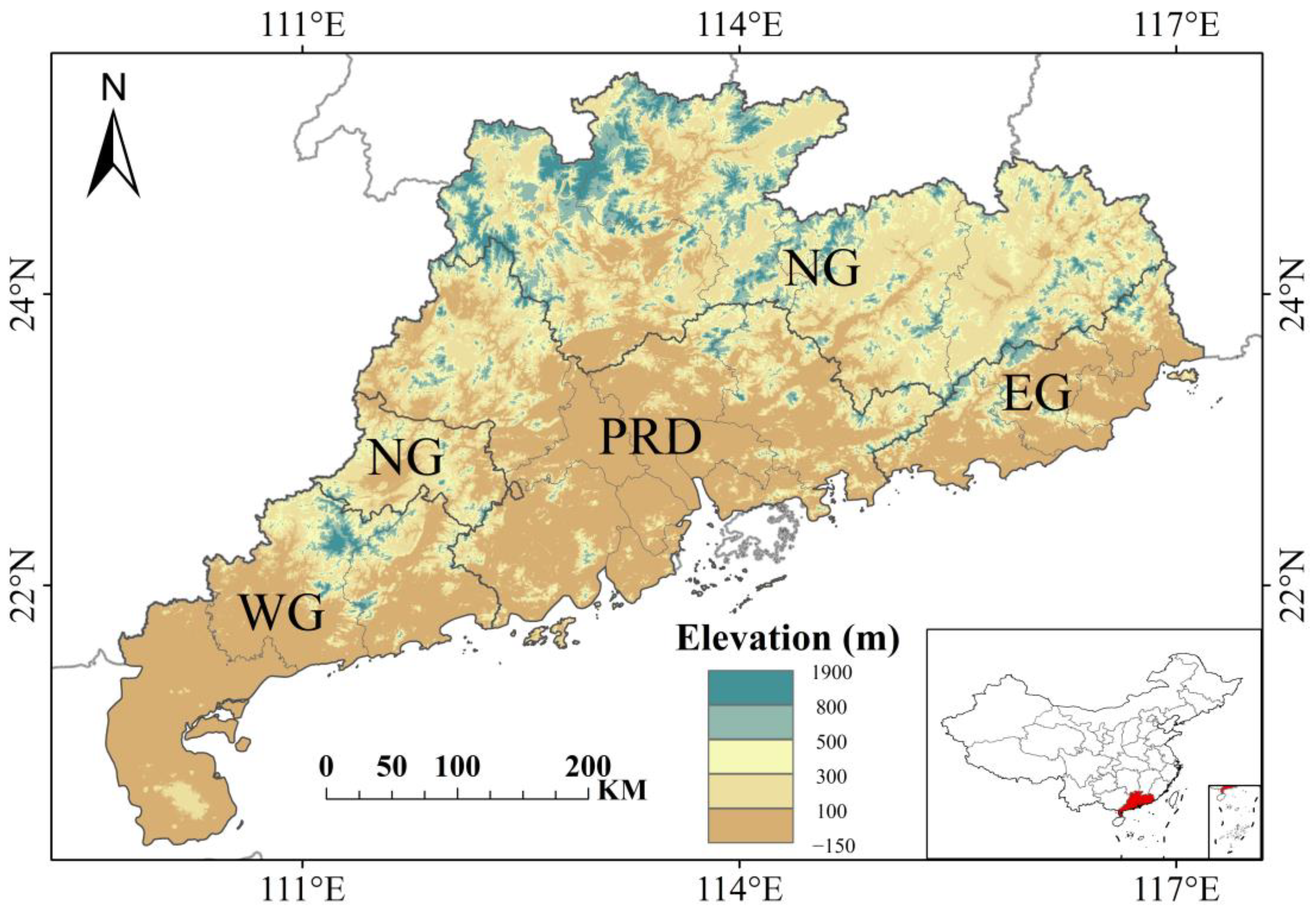
2.1. Study Area

Guangdong Province, situated in the southernmost part of mainland China (109°45′~117°20′E, 20°09′~25°31′N), covers approximately 17.97 million hectares of land. It is divided into 21 prefecture-level cities, typically categorized into four regions based on geographical location and economic conditions: the Pearl River Delta (PRD), Western Guangdong (WG), Northern Guangdong (NG), and Eastern Guangdong (EG) (Figure 1). The topography of Guangdong follows a north–south elevation pattern, predominantly featuring mountains and hills, with plains largely distributed in the southern coastal areas. The province experiences a tropical and subtropical monsoon climate with high humidity and precipitation. These favorable conditions lay the foundation for Guangdong’s status as a prominent agricultural province. According to the results of the third national land survey in 2019, Guangdong has 1.9019 million hectares of cropland. The wide variety of primary crops in the province includes rice, sugarcane, and peanuts. The cropping system in Guangdong is predominantly characterized by single cropping and double cropping and by triple cropping in a few areas, highlighting the complexity of the cropping systems [27].
However, ongoing and rapid urbanization processes in Guangdong have led to a substantial conversion of cropland to other land uses [28]. The increasing contradiction between rapid socio-economic development and the sharp decrease in the amount of cropland is becoming more pronounced. The complex natural conditions, flexible cropping systems, and the reduction in cropland due to economic development pose significant challenges for the monitoring of long-term cropland changes in Guangdong. Therefore, Guangdong is an excellent study area for monitoring changes in cropland.

2.2. Data and Pre-Processing

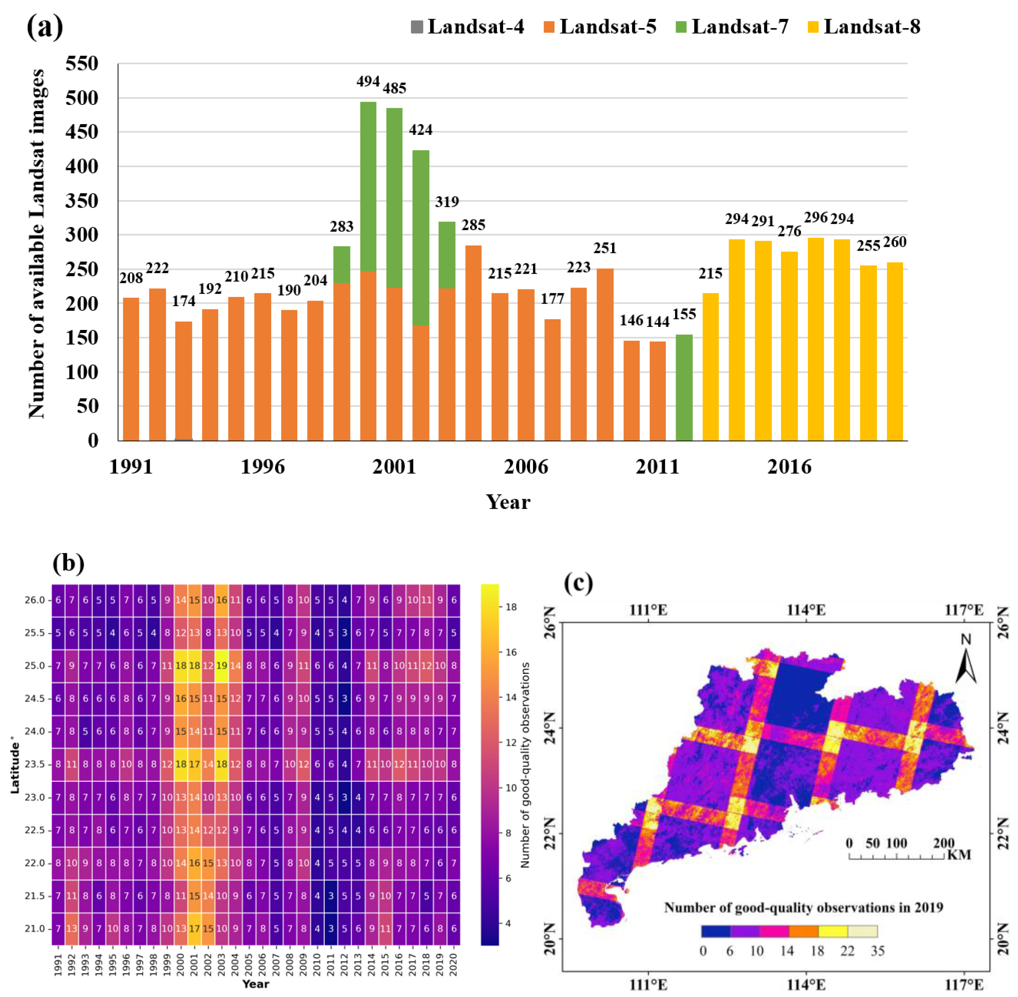
2.2.1. Landsat Imagery and Pre-Processing

The Landsat Program is a long-term remote sensing satellite program jointly proposed by NASA and the USGS [29]. Since the 1970s, Landsat has provided millions of observation images. We obtained a surface-reflectance (SR) dataset of Landsat images from GEE, which covers the province over 30 years. The data acquired from Landsat-7 ETM+ Scan Line Corrector exhibited striping issues [30]. Therefore, we only collected Landsat-7 images prior to 30 May 2003 and in 2012. The number of available images collected each year was consistently above 140. These data were calibrated and uniformly processed to the consistent L1TP level across different satellites. Figure 2a shows the annual availability of Landsat-4/5/7/8 images.
To improve data quality, we identified and masked clouds, cloud shadows, and snow pixels using the CFMask algorithm [31]. All data acquisition and processing were conducted within GEE. The annual quantity of high-quality observation images for Guangdong is shown in Figure 2, ensuring a minimum of 3 coverage images per 0.5° latitude for each year.

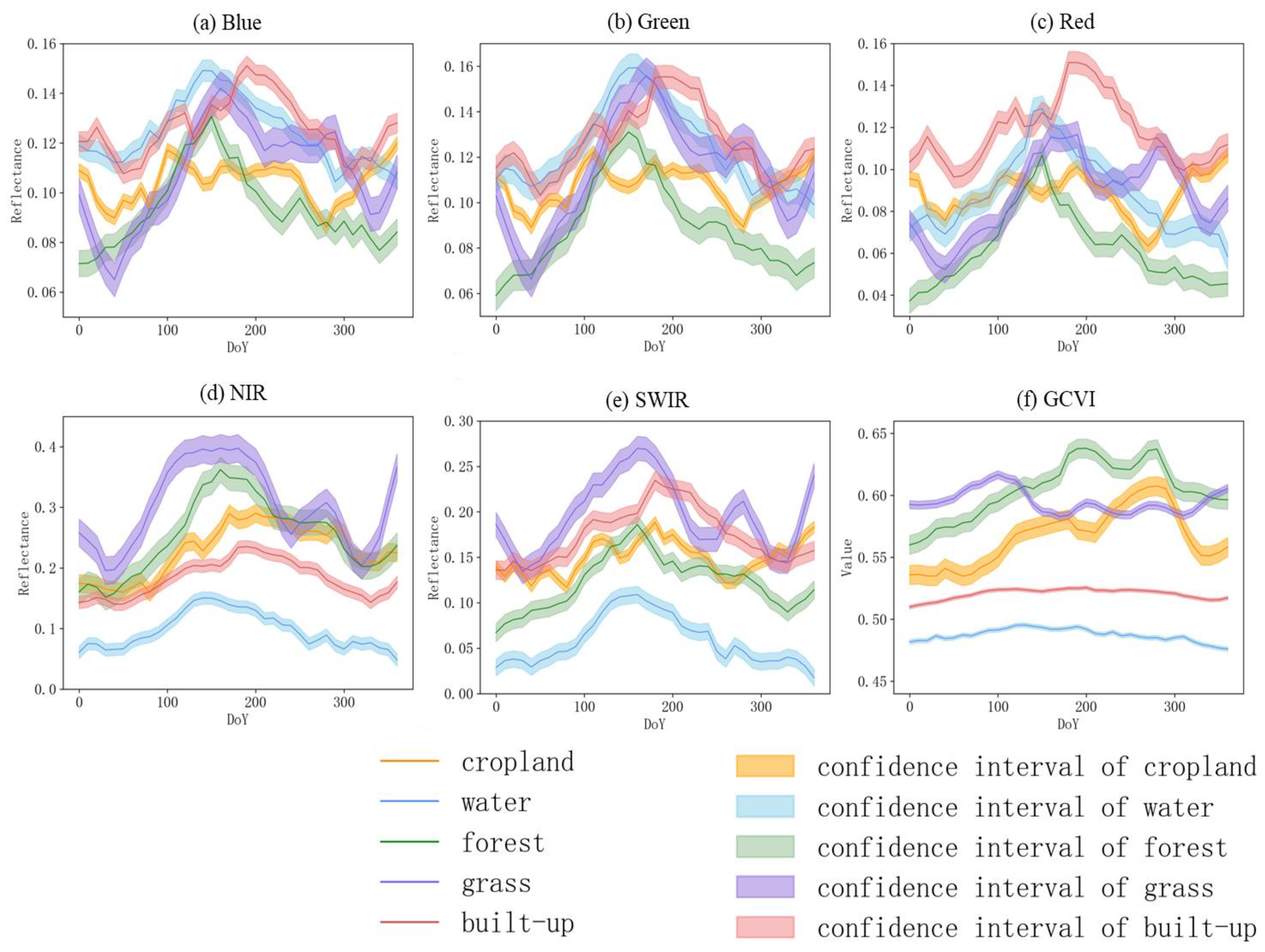
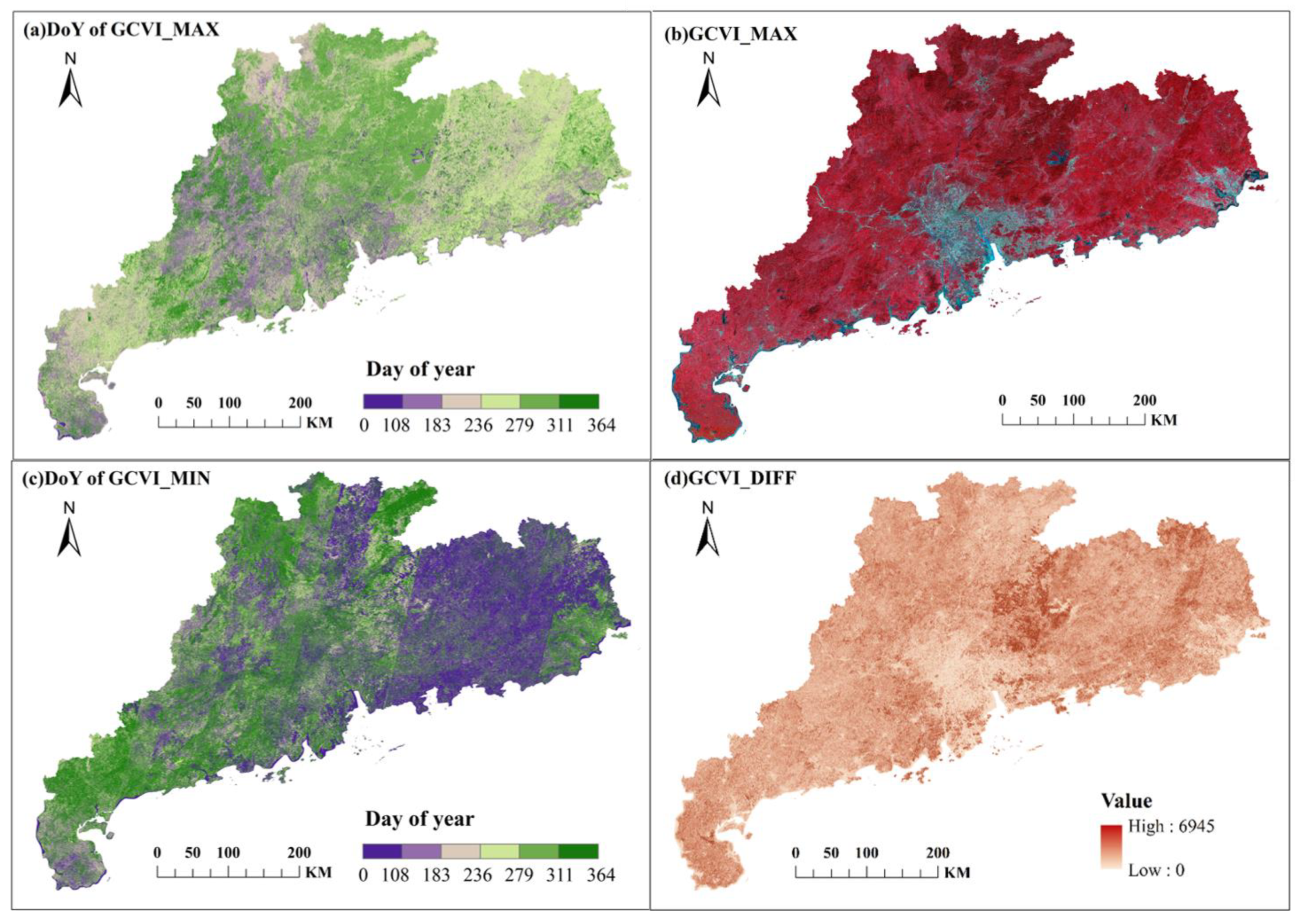
2.2.2. Vegetation Indices

Although the Green Chlorophyll Vegetation Index (GCVI) is not a widely used vegetation index, relevant research has shown that it has a roughly linear relationship with vegetation chlorophyll content and the Leaf Area Index (LAI) [32,33]. It can reflect the growth status and chlorophyll content of vegetation. Moreover, even when vegetation becomes highly dense, GCVI is not affected by the saturation of LAI in dense canopies and maintains relatively high sensitivity during periods of vigorous vegetation growth [34]. We used GCVI as a key index for distinguishing between different land use types with varying vegetation coverage in the study area, including grassland, cropland, and forest.
GCVI = ρ NIR ρ green 1

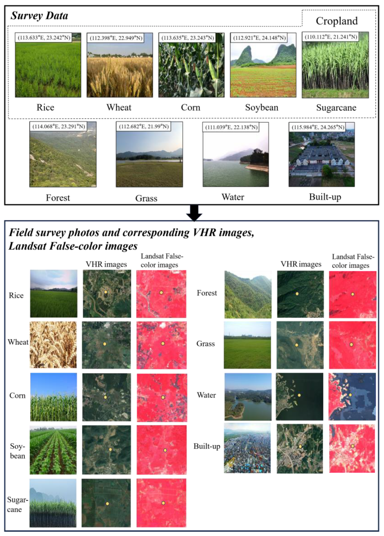
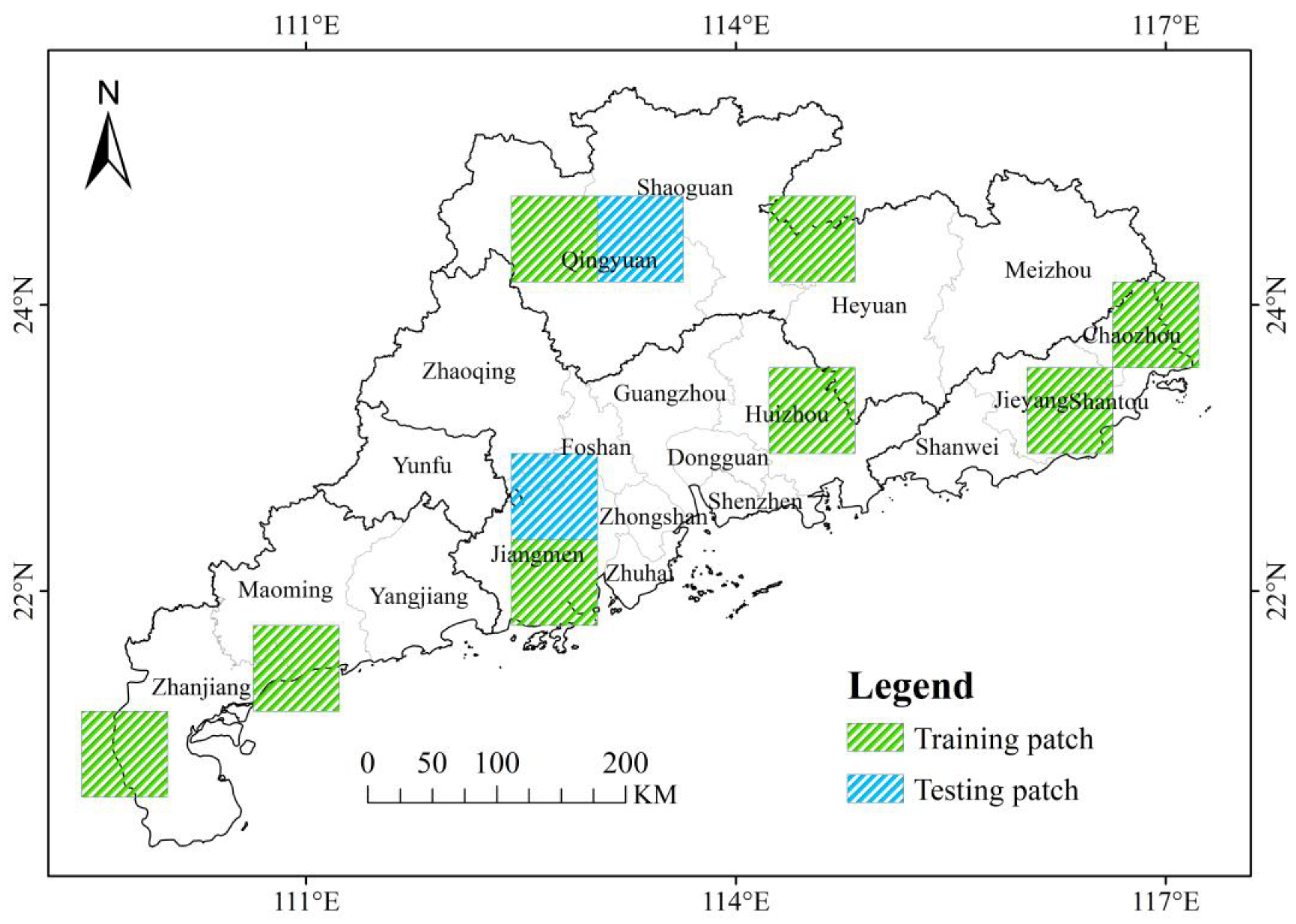
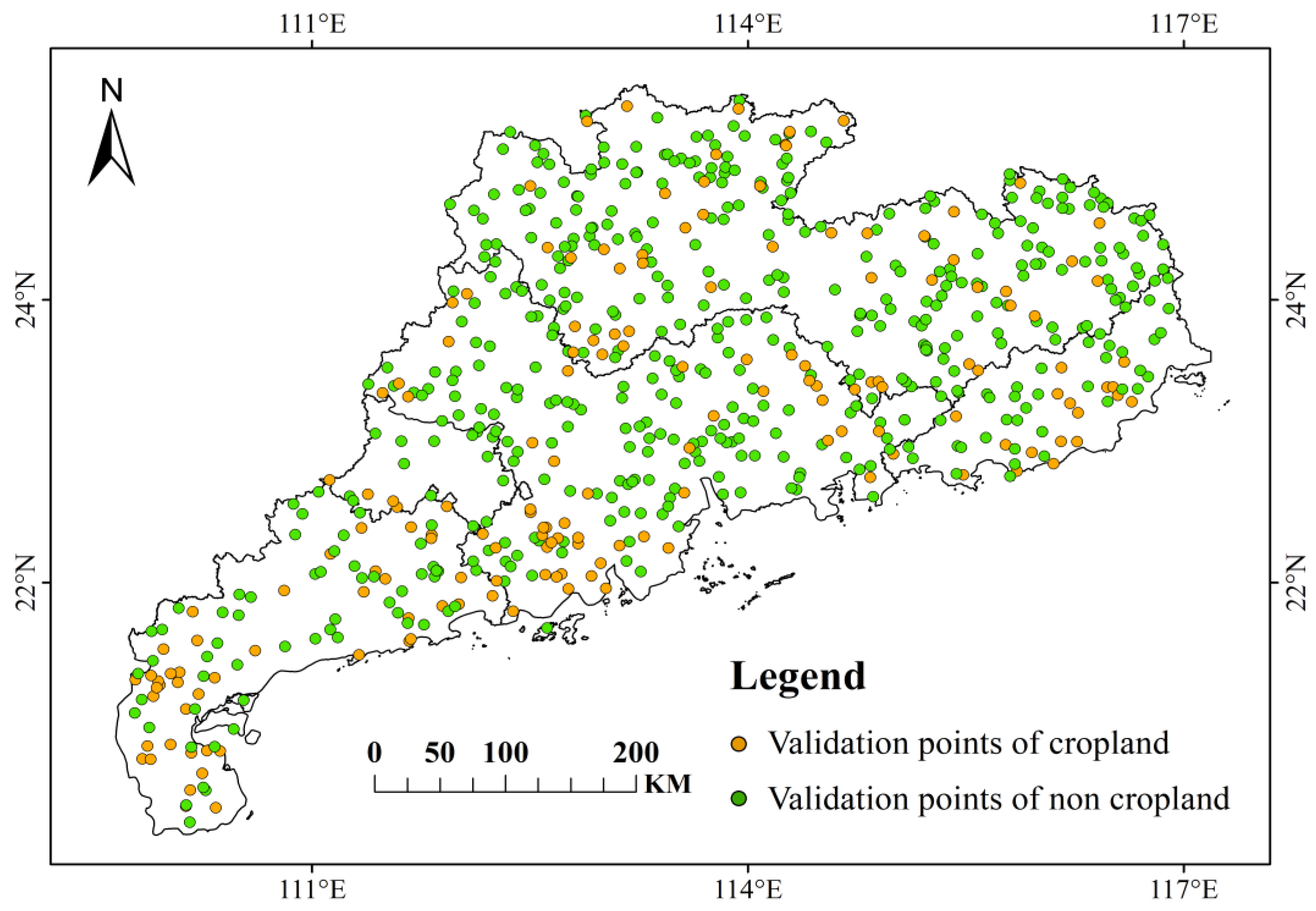
2.2.3. Field Survey and Sample Data

To understand the spectral characteristics of cropland in the study area, a field survey was conducted in Guangdong in 2019. The sample points for this survey were randomly distributed across different regions of Guangdong Province. These sample points encompassed five land use types: cropland, forest, grassland, water, and built-up land. Among them, cropland sample points primarily included typical crops in Guangdong, such as rice, wheat, corn, soybeans, and sugarcane. The visual interpretation marks and feature image library for typical land use types and crops in the study area were constructed based on the field survey data. This library included on-site photographs of sample points, very-high-resolution imagery, and Landsat false-color images (Figure 3).
We used the China Multi-Temporal Land Use and Land Cover Remote Sensing Monitoring Dataset (CNLUCC) and combined it with visual interpretation marks and a feature image library to generate labels for training and testing samples, which represent the actual ground conditions in 2019 [35]. When selecting the training and testing data, the following principles were followed. First, Guangdong was divided into numerous grid cells, each measuring 60 km × 60 km, and ten grids were selected as training and testing data. Considering the differences in cropland in each subregion of the study area, ten grids should be evenly distributed in the whole study area. Secondly, representative grids were selected for each subregion; these grids should contain extensive cropland areas and various cropping systems. The types of crops on cropland in these grids should be rich, and the proportion of cropland and other land use types should be relatively balanced. Finally, eight grids were randomly selected as training data, and two grids were selected as testing data (Figure 4).

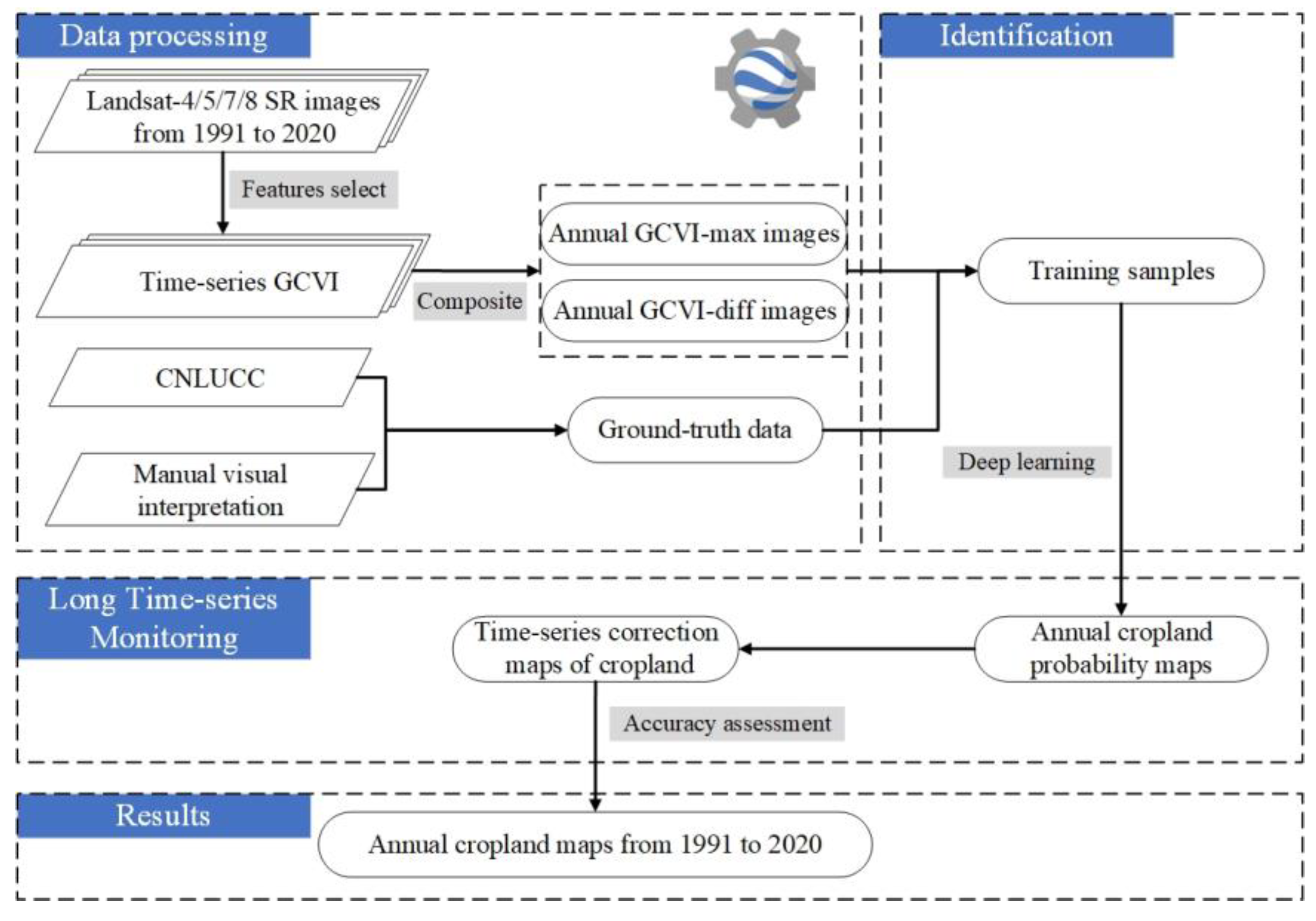
2.3. Algorithm for Monitoring Long Time Series of Cropland

Figure 5 provides a comprehensive overview of the long-time-series cropland monitoring algorithm presented in this study. We first selected all high-quality observation results based on the Landsat-4/5/7/8 SR images from 1991 to 2020. Subsequently, we extracted annual GCVI-max and GCVI-diff feature images from the GCVI time series. In addition, we collected ground-truth data using existing land use datasets and through manual visual interpretation, generating training samples for 2019. Next, we utilized deep learning techniques to predict the annual cropland probability map for Guangdong from 1991 to 2020. We corrected the unreasonable cropland changes in the long time series based on the LandTrendr algorithm. Finally, we evaluated the classification accuracy of the cropland map through validation samples and explored the changes in cropland in Guangdong from 1991 to 2020.

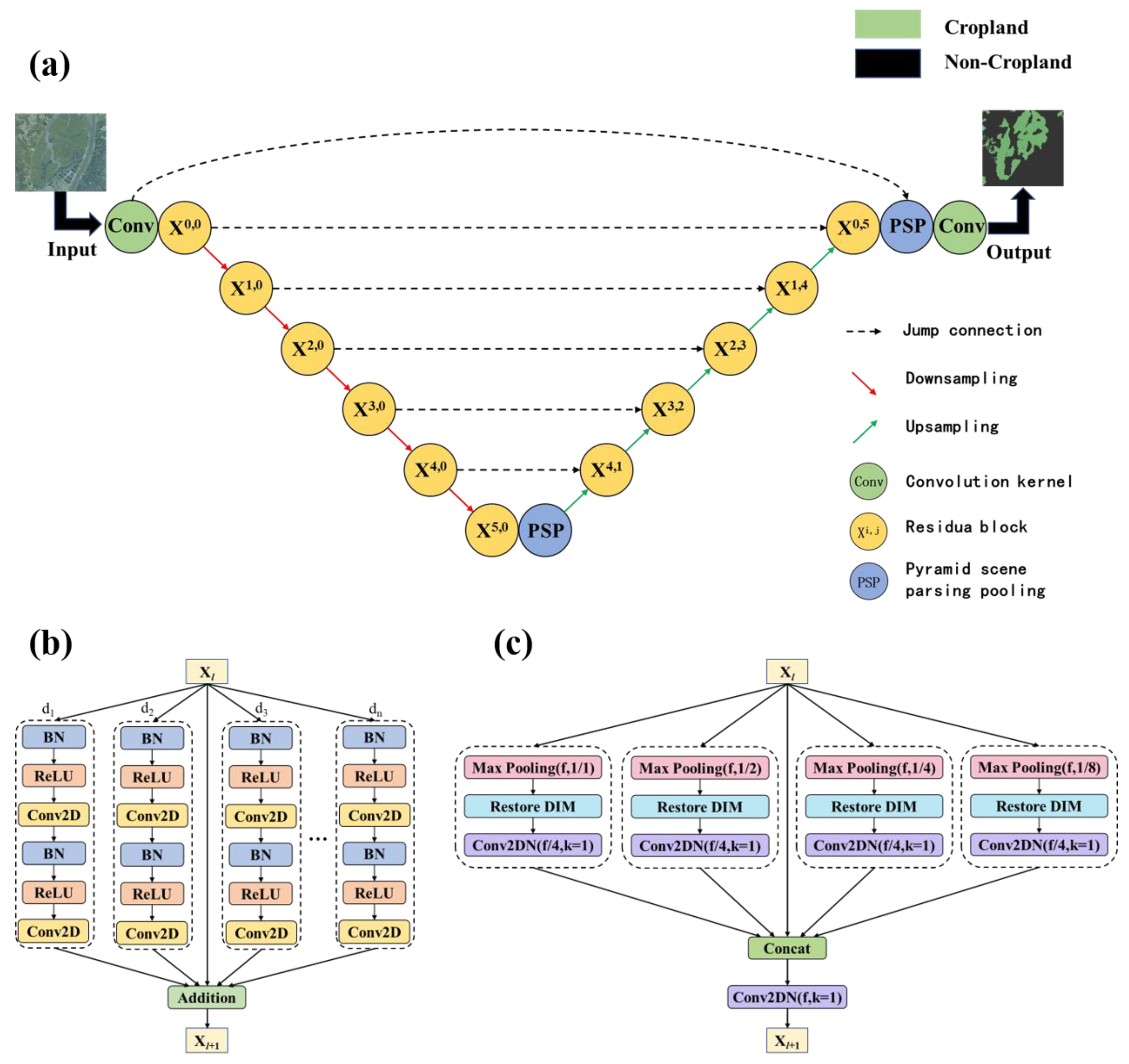
2.3.1. Algorithm for Cropland Identification

Due to the frequently cloudy and rainy weather in the study area, a significant number of pixels in Landsat images are covered by clouds or cloud shadows. Choosing a fixed-date image as the reference for cropland identification would inevitably lead to data loss. Simultaneously, the complex cropping system in Guangdong Province makes it challenging to extract phenological features of different vegetation based on a fixed time. Therefore, we were committed to finding a method to automatically determine key images for cropland identification from the spectral time-series data. The GCVI time-series curve effectively reflects the vegetation’s growth conditions at different periods. Both the maximum value and the difference between the maximum and minimum values of the curve can represent the physiological characteristics of vegetation. Therefore, our algorithm can identify the two crucial times of GCVI based on the time-series curve, encompassing both the maximum value and the maximum difference, without fixing the image date. It then extracts images corresponding to these two times. We combined this approach with deep learning techniques to achieve cropland identification in Guangdong from 1991 to 2020. The method fully utilizes all high-quality observational data within a year, reducing the impact of data gaps while extracting spectral features of various crops without considering complex crop types in the study area.
More specifically, we collected spectral data throughout 2019 and normalized all spectral indices. By observing the smoothed time series of spectral data, differences in time-series spectral curves for different land use types can be identified in the original bands. As shown in Figure 6, differences in phenological features between them can be reflected by observing the time-series curves of vegetation indices. Cropland experiences significant GCVI growth at around 100 days and decreases significantly after two growing seasons. Due to crop harvesting, cropland often transitions to the winter season with bare soil. Thus, the difference between GCVI during the growing season and non-growing season is significant. GCVI ranges from 0.53 to 0.6, with GCVI during the non-growing season being lower than that of forest and grassland. Forests in Guangdong are characterized by evergreen vegetation with high vegetation cover. Their GCVI is consistently higher than that of cropland, typically ranging from 0.55 to 0.65. Due to the region’s high temperature and abundant rainfall throughout the year, grassland maintains a certain level of vegetation cover year-round, resulting in minimal variation in GCVI, which fluctuates around 0.6. Water may experience slight seasonal fluctuations in GCVI, influenced by aquatic vegetation. Built-up land with some vegetation cover tends to have higher GCVI than water and generally remains relatively stable throughout the year, showing no significant fluctuations.
Due to the high sensitivity of GCVI during periods of vigorous vegetation growth, we can identify two key phenological periods by observing GCVI time-series curves. One of these key phenological periods is the “vegetation lush period” (VLP), which corresponds to the peak period of the GCVI curve. During this period, cropland can be significantly distinguished from water and built-up land and, to some extent, from forest as well. The other key phenological period is the “vegetation differential period” (VDP), which corresponds to the period with the greatest interannual differences in GCVI time series. During this period, cropland experiences significant changes in vegetation cover, while grassland exhibits relatively small changes, making it advantageous for distinguishing between cropland and grassland. We integrated high-quality observational data from each year, using the GCVI_MAX to generate the VLP images (Figure 7a,b). We also calculated the GCVI_diff, which represents the difference between the GCVI_MAX and the GCVI_MIN for each pixel to create the VDP images (Figure 7c,d).
GCVI _ diff = GCVI _ MAX GCVI _ MIN
The VLP and VDP images, combined with labeled data reflecting real ground conditions, were used as input to train the model. U-net is a typical convolutional neural network structure [36]. Its unique U-shaped network structure and jump connection mode can closely integrate shallow features with deep features, which not only significantly improves the feature extraction and generalization ability of the network but also reduces semantic gaps. This encoder–decoder structure can extract multi-scale features of cropland, fuse part of the lost information in the training process, and reduce training time and resources, so it has been widely used in land use classification research [37,38,39]. We employed ResUNet-a for cropland extraction, which addressed semantic gaps through skip connections [40]. To tackle gradient issues during training, U-Net’s building blocks were replaced with improved residual blocks. These blocks included multiple parallel atrous convolutions, allowing for adjustment of dilation rates to capture different receptive fields and extract features at various scales (Figure 8b). Additionally, pyramid scene parsing (PSP) pooling layers were introduced after the encoder and decoder stages to enhance the aggregation of contextual information and improve network performance (Figure 8c). Figure 8a provides an overview of the ResUNet-a architecture.

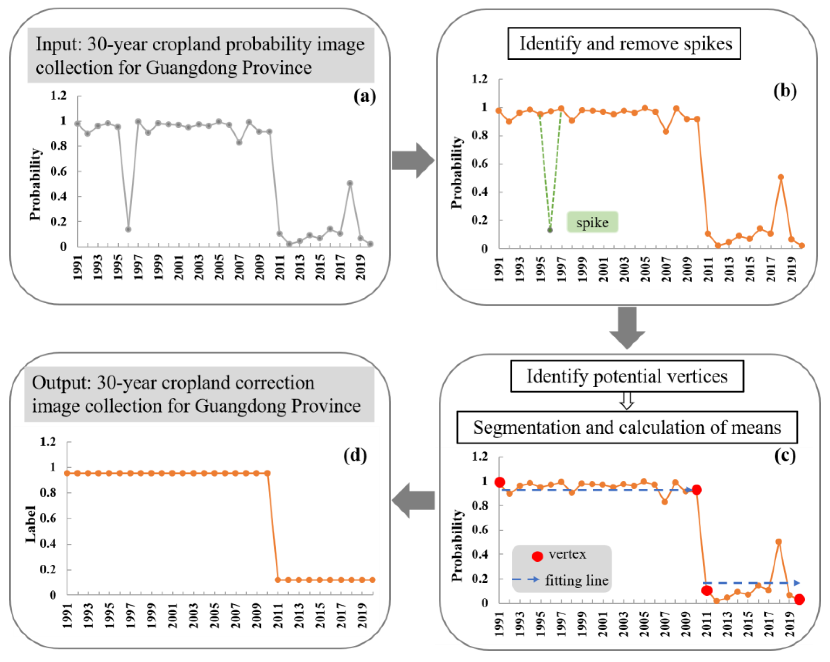
2.3.2. Algorithm for Long-Time-Series Cropland Correction

Cropland change is a long-term and complex process. When studying long-term cropland changes, it is essential to eliminate noise caused by image quality and accurately detect subtle variations. Identifying trends in slow and gradual vegetation cover changes is also important. The LandTrendr algorithm combines the advantages of traditional change detection methods for both capturing subtle changes and fitting trends in long time series. The algorithm uses an arbitrary segmentation approach, meaning it does not pre-establish an ideal model but, rather, utilizes basic data from long time series. It models important features with linear segments, which preserves critical details while eliminating noise. Originally, the LandTrendr algorithm was employed to study disturbances and recovery trends in forests [41]. Later, it became common for tracking changes and recovery in vegetation [42,43], water [44], and built-up land [45]. We developed the LandTrendr algorithm by leveraging its ability to detect abrupt and gradual changes. We introduced a long-time-series cropland correction algorithm, providing a comprehensive perspective for rectifying unreasonable variations in cropland predictions.
In our long-time-series cropland monitoring research, we conducted parameter tests while keeping other variables constant to find optimal values for the specific conditions of cropland changes in the study area. We established the operating parameters for the LandTrendr algorithm as shown in Table 1.
When there is a transition in land use between adjacent years, it is difficult to return to the previous state in the short term. However, noise-induced changes are temporary and can revert to the original state over time. We modeled the time series-predicted probability of pixels as a series of linear segments and eliminated the “spikes” caused by rapid changes between adjacent years due to noise. Following this, the residual-error criterion was employed to identify potential vertices. When the number of potential vertices exceeded the threshold, there may have been years in the fitting results that were not actually changed but were mistakenly identified as changes. We reconstructed the fitting lines by removing the vertex with the smallest angle. The ultimately confirmed vertices were identified as potential changes in land use between cropland and non-cropland. Between the vertices, we connected points in a point-to-point manner or perform fitting based on regression and simplified the model by removing the weakest vertices. During the fitting process, the p-values were used to control overfitting, and the optimal model was selected based on the smallest p-value. Once the optimal model was determined, the mean probability values within each segment were calculated to obtain the corrected probabilities of time series. The flow of the algorithm is shown in Figure 9.

2.4. Validation and Accuracy Assessment

To validate the accuracy of our algorithm in long-time-series cropland monitoring, we conducted stratified random sampling and accuracy assessment in Guangdong. We followed the recommended good practices for assessing forest area change and accuracy proposed by Olofsson [46]. We estimated the expected overall accuracy (OA) and assumed errors and determined an optimal sample size of 648 by repeatedly calculating the sample size. We proportionally and equally allocated the total sample size within the study area, examined accuracy and standard error estimates, and found the optimal sample size between these two allocation methods. In the end, we settled on 160 cropland sample points and 488 non-cropland sample points. Due to the significant spatial heterogeneity of cropland distribution in the study area, we randomly distributed sample points in four subregions according to their areas.
The stratified random sampling process was conducted in GEE. Using cropland identification results as the basis and 30 × 30 m pixels as the sampling units, we randomly generated sample points according to the calculated sample number in the two layers of cropland and non-cropland in the prediction results based on the stratified random sampling method in GEE. Table 2 displays the number of sample points in each subregion, and Figure 10 shows the distribution of these sample points. Considering variations between Landsat sensors, it is not sufficient to rely solely on accuracy validation results from a single year. Therefore, the validation process was conducted every 5 years over a 30-year period. Based on the confusion matrices of validation results, we calculated the overall accuracy (OA), user’s accuracy (UA), producer’s accuracy (PA), and the Kappa coefficient as evaluation metrics for cropland monitoring accuracy.

3. Results

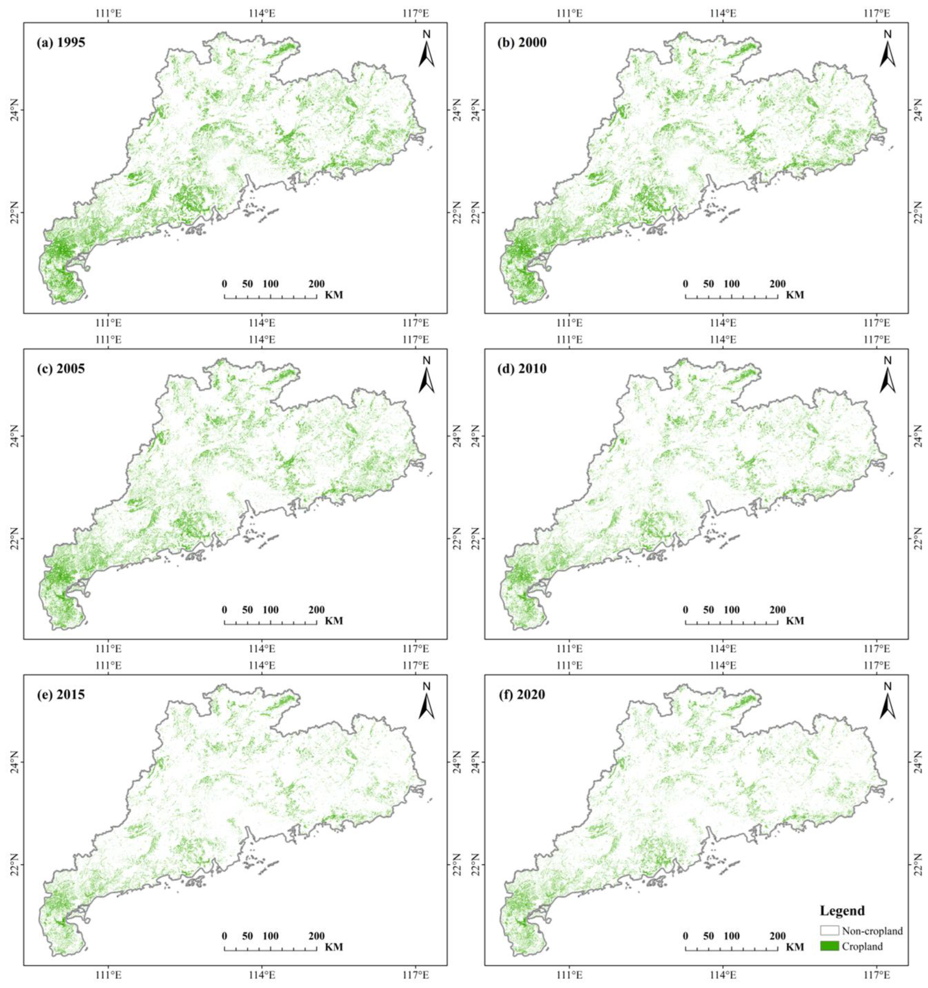
3.1. Results of Annual Cropland Map Assessment from 1991 to 2020

Based on the cropland identification result from 2020, we can observe from Table 3 that OA in all four subregions of Guangdong consistently exceeds 0.9. However, there was significant variation in Kappa among these subregions, and UA for cropland was lower compared to non-cropland. Notably, the highest accuracy was achieved in Eastern Guangdong (OA = 0.95, Kappa = 0.88), while the Pearl River Delta and Western Guangdong exhibited lower Kappa values (Kappa = 0.78), and Eastern Guangdong had a slightly lower OA (OA = 0.91). Several factors contributed to these variations. The Pearl River Delta region has a high degree of cropland fragmentation, which presented challenges in accurately identifying cropland. Northern Guangdong is characterized by hilly and mountainous terrain, with forests mostly concentrated at higher elevations, leading to similar spectral characteristics between forests and cropland. Western Guangdong features extensive orchards, with spectral features closely resembling those of croplands, resulting in potential confusion between the two land types. Eastern Guangdong, located in the Chaoshan Plain, boasts flat terrain with a more regular distribution of cropland. The varying distribution, shape, and cropping patterns of cropland in different subregions contributed to differences in cropland identification accuracy to some extent.
We present the detailed spatial distribution of cropland in Guangdong at five-year intervals from 1991 to 2020 in Figure 11. Reduction in cropland is most pronounced in the Pearl River Delta and Western Guangdong; other regions also witnessed varying degrees of cropland reduction. From the accuracy assessment results in Table 4, it is evident that OA values for all 6 years were above 0.9, and the Kappa remained above 0.8. This indicates that our method held great potential for long-term cropland monitoring. The highest OA was 0.93 (2005, 2015, 2020), while the lowest was 0.91 (1995, 2000). The highest Kappa was 0.83 (1995, 2005), while the lowest was 0.80 (2015). Overall, the accuracy was highest in 2015, possibly due to a significantly higher PA for 2005 compared to other years. UA for CL ranged from 0.80 to 0.85, with PA ranging from 0.79 to 0.92. UA for N-CL ranged from 0.93 to 0.96, with PA ranging from 0.93 to 0.95. Both UA and PA for N-CL were higher than those for CL.

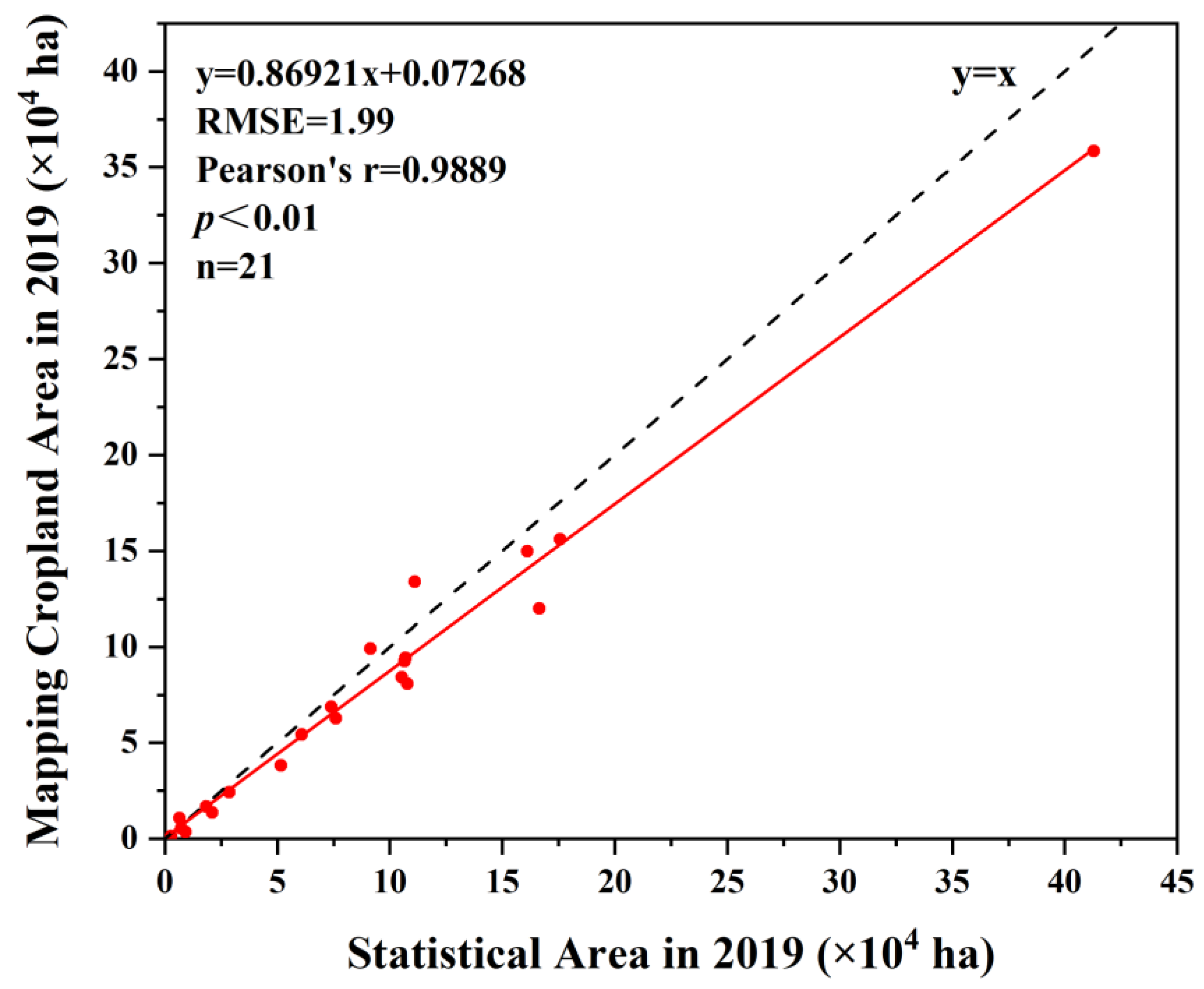
3.2. Results of Comparison with the Agricultural Statistical Data

Based on the 2019 cropland map of Guangdong, we estimated cropland areas for 21 prefecture-level cities and compared them with the cropland areas reported in the national agricultural statistical data for 2019. The results of Pearson correlation analysis indicated a highly significant linear relationship between cropland area in Guangdong and the national agricultural statistical data (slope = 0.870, Pearson’s r = 0.989, p < 0.01, RMSE = 1.99 × 10⁴ ha) (Figure 12). Apart from a few individual cities, the cropland area in our map is slightly lower than the national agricultural statistics. This variation may be attributed to various factors. Firstly, the methods of survey are different, and there are variations in survey principles. Furthermore, compared to Landsat imagery, land use surveys within rural and urban areas typically use imagery with resolutions superior to 0.2 m or 1 m as reference data. As a result, our data errors were within an acceptable range.

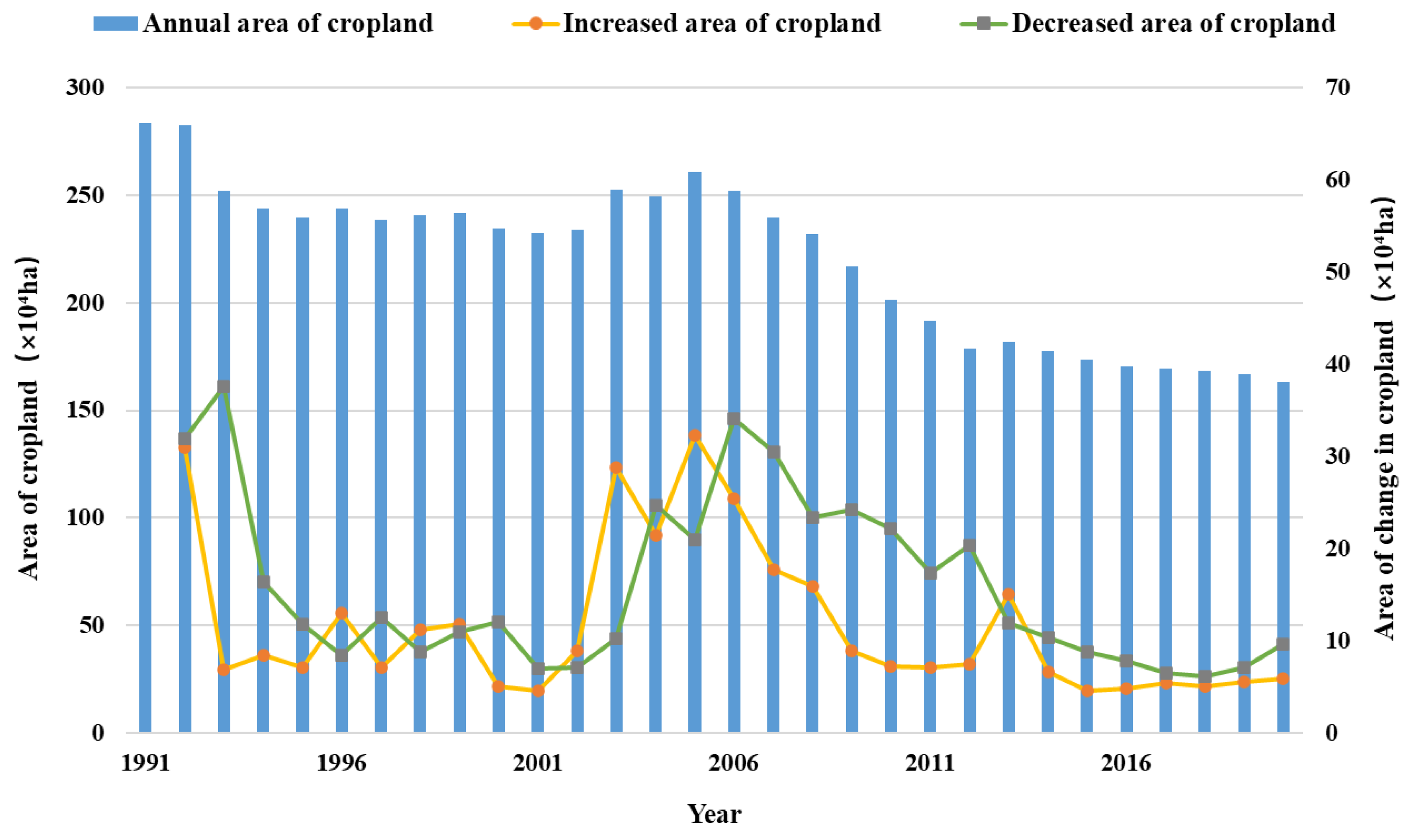
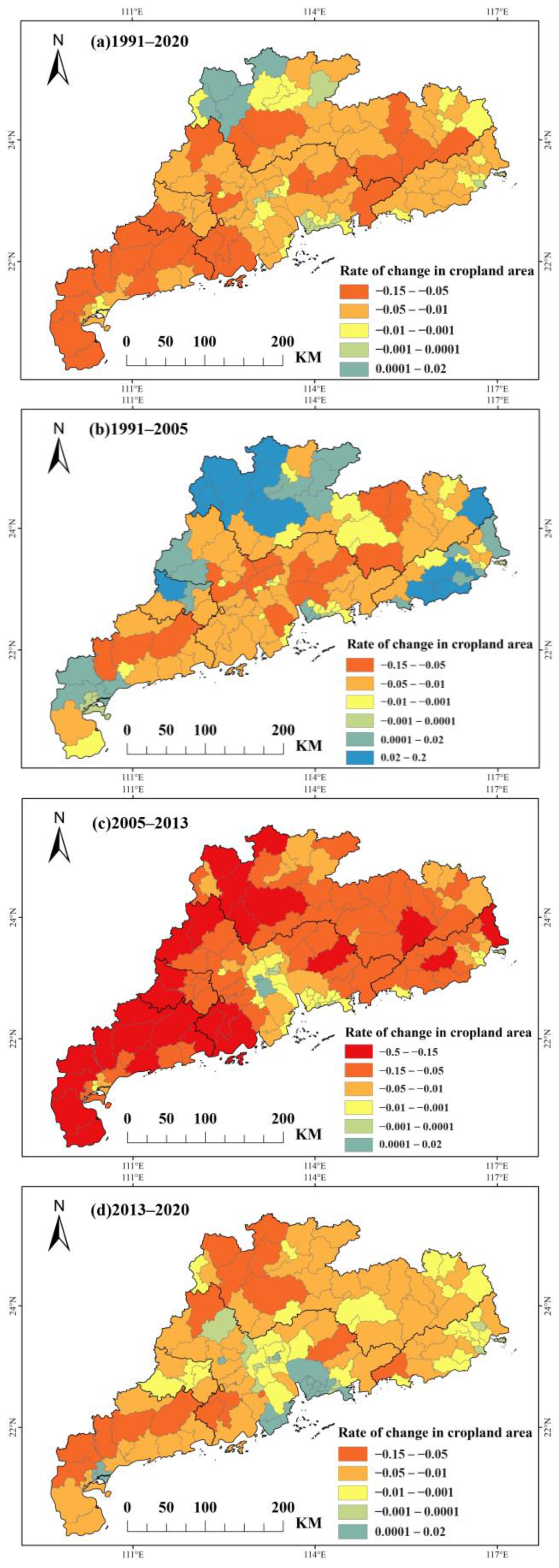
3.3. Assessment of Changes in Cropland Area from 1991 to 2020

Figure 13 displays the 30-year trend in the total cropland area for the province, highlighting changes in areas of increase and decrease. Over this period, there was an overall decreasing trend in the cropland area across the province, declining from 2,837,500 hectares in 1991 to 1,631,400 hectares in 2020, representing a reduction of approximately 42.5%. Two significant periods of decline stand out. The first decrease occurred in the early 1990s. China’s reform and opening-up policy led to the emergence of “Development Zone Boom” and “Real Estate Boom” [47,48], resulting in a nearly 10.9% decrease in cropland area in Guangdong in 1993. The second significant period occurred between 2005 and 2013. With the development of the economy, a new wave of “Urbanization Boom” also led to a reduction of 823,600 hectares of cropland.
Observing the curves of cropland increase and decrease, it became evident that in 1993, there was a peak in cropland expansion within the thirty-year period. From 1994 to 2002, the change in cropland area, including both additions and reductions, was relatively balanced. Notably, between 2003 and 2005, the conversion of non-cropland into cropland significantly increased, reflecting the development of cropland protection policies in the early 21st century. From 2013 to 2020, Guangdong experienced a period of relatively stable changes in cropland area, achieving a balance between cropland conversion and preservation.
Figure 14 illustrates the changes in cropland over 30 years in various county-level administrative regions of Guangdong. Overall, there was a significant overall decrease in the cropland area in Guangdong, with the most substantial reductions occurring in Western Guangdong and eastern parts of Northern Guangdong. However, there were slight additions of cropland in specific regions, mainly in Northern Guangdong. The 30-year changes in cropland in Guangdong can be divided into three distinct periods. From 1991 to 2005, the northern and southeastern parts of Guangdong experienced a notable increase in cropland. Meanwhile, other regions showed a continuing decrease in cropland (Figure 14b). From 2005 to 2013, the entire province witnessed a significant decrease in cropland. This decline was most pronounced in the western part of Guangdong, western regions of Northern Guangdong, parts of the Pearl River Delta, and some areas in southeastern Guangdong (Figure 14c). From 2013 to 2020, the rate of cropland reduction in Guangdong slowed down overall. Some regions, such as Western Guangdong and certain parts of Northern Guangdong, continued to experience a decrease in cropland. Conversely, the northern part of the Pearl River Delta showed an increasing trend in cropland area (Figure 14d).

4. Discussion

4.1. Advantages of Our Algorithms

In existing research on long-term cropland changes, systematic cropland change monitoring offers a more comprehensive way to assess annual variations in cropland compared to methods involving the overlaying of annual cropland maps or updating changes based on reference years. It helps avoid cumulative errors over time. However, previous systematic cropland monitoring studies typically fall into two categories: they either focus on deviations, capturing abrupt cropland change events from subtle distinctions between adjacent years or they concentrate on cropland change trends, seeking out long-term and gradual changes within complete time series. Our algorithm, in contrast, takes an integrated approach by considering the potential for both short-term, abrupt changes and long-term, gradual evolution in cropland. It investigates cropland change trends while making every effort to eliminate spurious changes. Only continuous and reasonable data between years reflect the real situation of interannual variation of cropland, so the long-time-series cropland dataset based on our algorithm can be applied to the analysis of continuous interannual variation of cropland in practice.
One of the significant factors contributing to spurious changes is image quality. Our algorithm made extensive use of high-quality Landsat observations obtained each year, automatically generating feature-enhanced images for two critical phenological periods: VLP and VDP. This ensured data consistency year after year and reduced spurious changes resulting from spectral variations. Furthermore, our algorithm addressed the issue of fluctuating identification results between cropland and non-cropland in adjacent years due to mixed pixels. This correction, to some extent, minimized the uncertainty in identification results caused by data quality.

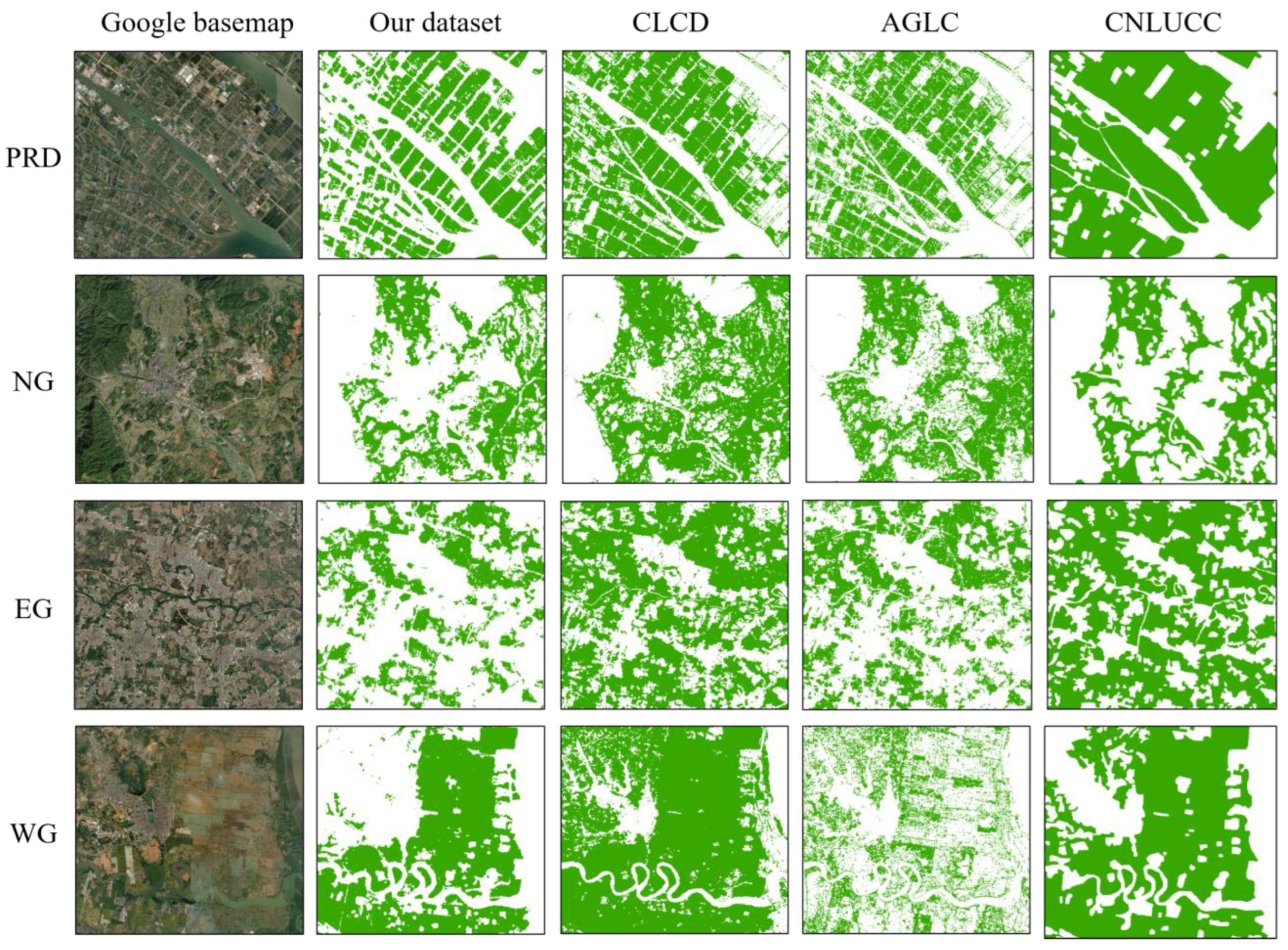
4.2. Comparison with Different Datasets

To evaluate the advantages of our dataset, we selected three existing land use/land cover datasets with a temporal overlap in the year 2015 and extracted cropland from them for comparison with our proposed dataset. These datasets included the China Land Cover Dataset (CLCD) [26], as well as the Annual Global Land Cover (AGLC) [49] and China Land Use and Land Cover Change (CNLUCC) datasets. We specifically selected contiguous cropland areas in four subregions for comparison. Overall, the distribution of cropland in these four datasets exhibited consistency.
To assess accuracy and differences between different datasets, we randomly generated a uniformly distributed set of validation points across the four datasets. As shown in Table 5, our dataset outperformed the other three, with the highest OA and Kappa. All six evaluation metrics were above 0.9, indicating our dataset’s high accuracy. However, because of overestimation of cropland area, CNLUCC exhibited the most severe misclassification of cropland, with a substantial omission of cropland. AGLC also had significant misclassification and omission issues. While CLCD’s overall classification was better than that of the other two datasets, its classification accuracy is still not ideal. Although CLCD, AGLC, and CNLUCC are national or global products, the accuracy assessment suggested that large-scale cropland cover mapping products, although generally accurate, do not perform well in areas with fragmented cropland distribution and complex cropping systems. This underscores the necessity of conducting cropland identification research in Guangdong, which exhibited complex cropland characteristics.
In more detail, CLCD and AGLC are both pixel-based annual land use classification products, leading to fragmented identification results for cropland. CLCD has the largest cropland area among the four datasets because it might misclassify smaller areas of forest, built-up land, and ponds as cropland. Moreover, it was insensitive to the boundaries between cropland and built-up land, leading to the overestimation of cropland area. The results of cropland identification of AGLC were more detailed and more sensitive to cropland boundaries, making it the smallest of the four datasets in terms of cropland area. However, because AGLC is a global land cover product, it was constrained by the number of samples. It substantially underestimated cropland area in the complex cropland distribution of the Western Guangdong region (Figure 15). CNLUCC is based on remote sensing imagery and human–machine interaction, which resulted in a relatively accurate spatial distribution of cropland. However, it had coarse boundaries and could not effectively identify fragmented cropland. There were also instances of misclassification of areas of built-up land between cropland, leading to an overall overestimation of cropland area. Additionally, human–machine interaction products require substantial manual effort for updates, making annual updates challenging. In contrast, our dataset is an annual cropland product that does not require substantial manual labor for timely, long-term, dynamic monitoring of cropland. Furthermore, we used an object-based approach, which allowed for a more accurate distinction of boundaries between cropland and built-up land. Cropland geometries were more regular in our dataset, giving it a significant advantage in cropland identification at the plot scale.

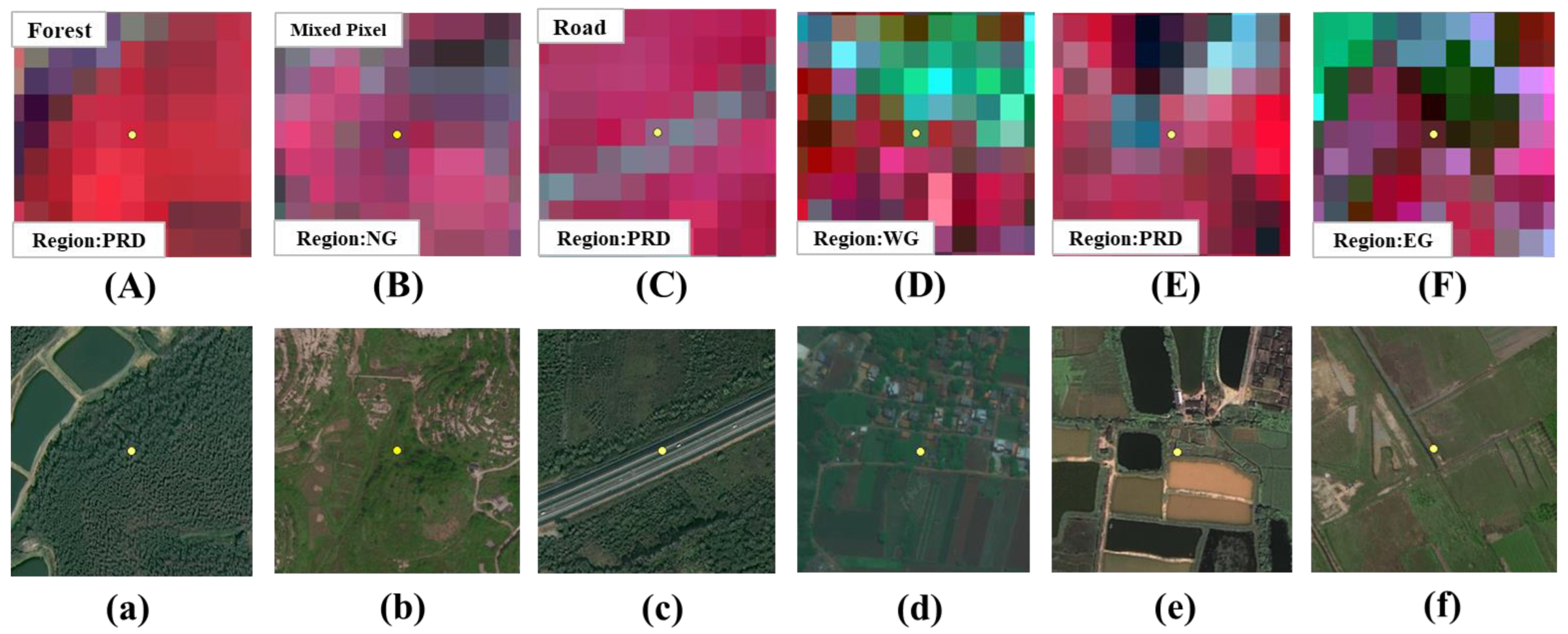
4.3. Uncertainty of the Algorithm and Misclassification of the Validation

Mapping large-scale cropland distribution and monitoring long-term changes in cropland pose significant challenges. In this study, several factors influenced our monitoring results. First, despite our utilization of Landsat-4/5/7/8 imagery from every year over a thirty-year period, data gaps were still inevitable. The 16-day revisit cycle was insufficient for conducting long-time-series studies, and the issue of data striping in Landsat-7 reduced the quantity of high-quality observational data. During the rainy and cloudy season, there could be continuous months with a lack of valid data, and the quality of the data would affect the accuracy of identification. Secondly, the 30 m spatial resolution reduced mixed-pixel effects to some extent. However, due to the fragmented landscape pattern in Guangdong, accurately depicting the roads between cropland and the buildings near cropland remained challenging. When some cropland is specially used, our algorithm will also experiences some limitations. For example, if fruit trees are planted in cropland year-round or if the cropland is covered by greenhouses throughout the year, cropland may be identified as non-cropland.
In stratified random sampling validation, our cropland map exhibited some occasional classification errors (Figure 16). Among these, cropland was occasionally confused with forests and roads. Considering the dense forest cover in the study area, it is, indeed, challenging to completely differentiate cropland based on phenological features and geometric shapes, leading to common misclassifications (Figure 16A,a). In areas where forests are adjacent to cropland, the boundary between the two land types may not be obvious (Figure 16B,b). Furthermore, roads between larger cropland plots were not consistently separated from cropland, and such commission errors occur less frequently (Figure 16C,c). In our results, there were also some omission errors, which often occurred at the interface between cropland and built-up land (Figure 16D,E,d,e). These mentioned classification errors serve as a test of the neural network’s edge extraction capabilities and are areas of further research focus.

4.4. Implications and Future Work

As a pioneer in the reform and opening up, Guangdong has experienced rapid economic growth in recent years. However, agriculture has been significantly affected, with a large amount of cropland being converted into built-up land or other land use types. Therefore, monitoring cropland changes in Guangdong and creating precise, long-term cropland maps hold significant importance for safeguarding food security and monitoring cropland areas. In the face of the complex terrain and cropland characteristics of southern China, the long-time-series cropland monitoring algorithm we have proposed can achieve extensive and long-term cropland change monitoring in the South China region. In conclusion, achieving more precise cropland identification and change monitoring requires the attainment of specific phenological information relevant to the study area. Such information varies due to differences in latitude, longitude, and elevation, leading to regional disparities. In our future work, we will aim to apply this methodology nationwide and potentially globally. This may involve delving into more complex phenological features to optimize our algorithm, and we need to add a small number of samples with characteristics that differ from those of cropland in Guangdong Province. Additionally, we can explore seasonal changes in cropland throughout a year.

5. Conclusions

With the rapid development of the economy in recent decades, great changes have taken place in the distribution and area of cropland in Guangdong Province. Exploring the distribution and change in cropland and realizing long-time-series monitoring is of great significance in studying the driving mechanism of cropland change and formulating protection policies. However, due to the impacts of data quality and monitoring methods, achieving accurate long-term, interannual monitoring of cropland has been a challenging task. Most existing remote sensing cropland monitoring datasets do not take into account the rationality of interannual variation of cropland, so they are difficult to apply to actual scenarios. In this study, we developed a long-time-series cropland monitoring algorithm that can correct unreasonable interannual changes in cropland and carried out good practice in South China, which is characterized by cloudy and rainy conditions, complex cropping systems, and a high degree of cropland fragmentation. The results indicate that the cropland monitoring results in Guangdong Province over a period of 30 years exhibit high accuracy, with an OA of 0.80–0.83 and Kappa coefficients of 0.91–0.93. These results are also highly consistent with agricultural statistical data. The overall trend in cropland area in Guangdong Province has shown a decrease over the 30-year period, with variations in trends observed in different regions and periods. Our method monitors cropland from the perspectives of long-term, gradual change and short-term, abrupt change, which not only partially overcoming the uncertainties present in traditional cropland monitoring methods but also providing accurate information on cropland spatial distribution and area changes. These data serve as crucial foundational information for agricultural production and cropland conservation. Moreover, since the 30-year cropland dataset has a high degree of continuity between years, it can be used to analyze the long-term, interannual changes in cropland in real scenarios. Future research could expand to larger regions and delve into more detailed changes in cropland during the year.

Author Contributions

Conceptualization, L.L. and Y.Q.; methodology, L.L., Y.Q. and H.X.; software, Y.Q. and H.X.; validation, B.Z.; formal analysis, Y.Q. and B.Z.; investigation, B.Z. and H.X.; resources, L.L. and Z.Q.; data curation, L.L. and Z.Q.; writing—original draft preparation, Y.Q.; writing—review and editing, Y.Q., B.Z., L.L., H.X. and Z.Q.; visualization, Y.Q. and B.Z.; supervision, L.L.; project administration, L.L.; funding acquisition, L.L. All authors have read and agreed to the published version of the manuscript.

Funding

This research was funded by the Common Application Support Platform for National Civil Space Infrastructure Land Observation Satellites (Grant Number 2017-000052-73-01-001735).

Data Availability Statement

The cropland maps in this study are available from the corresponding author upon reasonable request.

Acknowledgments

The authors want to thank the editor, associate editor, and anonymous reviewers for their helpful comments and advice.

Conflicts of Interest

The authors declare no conflicts of interest.

References

  1. Liu, B.; Song, W. Mapping Abandoned Cropland Using Within-Year Sentinel-2 Time Series. Catena 2023, 223, 106924. [Google Scholar] [CrossRef]
  2. Abass, K.; Adanu, S.K.; Agyemang, S. Peri-Urbanisation and Loss of Arable Land in Kumasi Metropolis in Three Decades: Evidence from Remote Sensing Image Analysis. Land Use Policy 2018, 72, 470–479. [Google Scholar] [CrossRef]
  3. Yuan, Z.; Zhou, L.; Sun, D.; Hu, F. Impacts of Urban Expansion on the Loss and Fragmentation of Cropland in the Major Grain Production Areas of China. Land 2022, 11, 130. [Google Scholar] [CrossRef]
  4. Gao, R.; Chuai, X.; Ge, J.; Wen, J.; Zhao, R.; Zuo, T. An Integrated Tele-Coupling Analysis for Requisition–Compensation Balance and Its Influence on Carbon Storage in China. Land Use Policy 2022, 116, 106057. [Google Scholar] [CrossRef]
  5. Zheng, Q.; Siman, K.; Zeng, Y.; Teo, H.C.; Sarira, T.V.; Sreekar, R.; Koh, L.P. Future Land-Use Competition Constrains Natural Climate Solutions. Sci. Total Environ. 2022, 838, 156409. [Google Scholar] [CrossRef]
  6. Ridoutt, B.; Navarro Garcia, J. Cropland Footprints from the Perspective of Productive Land Scarcity, Malnutrition-Related Health Impacts and Biodiversity Loss. J. Clean Prod. 2020, 260, 121150. [Google Scholar] [CrossRef]
  7. Xu, Y.; Yu, L.; Zhao, F.R.; Cai, X.; Zhao, J.; Lu, H.; Gong, P. Tracking Annual Cropland Changes from 1984 to 2016 Using Time-Series Landsat Images with a Change-Detection and Post-Classification Approach: Experiments from Three Sites in Africa. Remote Sens. Environ. 2018, 218, 13–31. [Google Scholar] [CrossRef]
  8. Leroux, L.; Jolivot, A.; Bégué, A.; Seen, D.; Zoungrana, B. How Reliable Is the MODIS Land Cover Product for Crop Mapping Sub-Saharan Agricultural Landscapes? Remote Sens. 2014, 6, 8541–8564. [Google Scholar] [CrossRef]
  9. Zhu, C.; Lu, D.; Victoria, D.; Dutra, L. Mapping Fractional Cropland Distribution in Mato Grosso, Brazil Using Time Series MODIS Enhanced Vegetation Index and Landsat Thematic Mapper Data. Remote Sens. 2015, 8, 22. [Google Scholar] [CrossRef]
  10. Wambugu, N.; Chen, Y.; Xiao, Z.; Wei, M.; Aminu Bello, S.; Marcato Junior, J.; Li, J. A Hybrid Deep Convolutional Neural Network for Accurate Land Cover Classification. Int. J. Appl. Earth Obs. Geoinf. 2021, 103, 102515. [Google Scholar] [CrossRef]
  11. Xie, D.; Xu, H.; Xiong, X.; Liu, M.; Hu, H.; Xiong, M.; Liu, L. Cropland Extraction in Southern China from Very High-Resolution Images Based on Deep Learning. Remote Sens. 2023, 15, 2231. [Google Scholar] [CrossRef]
  12. Wu, S.; Su, Y.; Lu, X.; Xu, H.; Kang, S.; Zhang, B.; Hu, Y.; Liu, L. Extraction and Mapping of Cropland Parcels in Typical Regions of Southern China Using Unmanned Aerial Vehicle Multispectral Images and Deep Learning. Drones 2023, 7, 285. [Google Scholar] [CrossRef]
  13. Zhang, D.; Pan, Y.; Zhang, J.; Hu, T.; Zhao, J.; Li, N.; Chen, Q. A Generalized Approach Based on Convolutional Neural Networks for Large Area Cropland Mapping at Very High Resolution. Remote Sens. Environ. 2020, 247, 111912. [Google Scholar] [CrossRef]
  14. Yin, H.; Brandão, A.; Buchner, J.; Helmers, D.; Iuliano, B.G.; Kimambo, N.E.; Lewińska, K.E.; Razenkova, E.; Rizayeva, A.; Rogova, N.; et al. Monitoring Cropland Abandonment with Landsat Time Series. Remote Sens. Environ. 2020, 246, 111873. [Google Scholar] [CrossRef]
  15. Xu, Y.; Yu, L.; Cai, Z.; Zhao, J.; Peng, D.; Li, C.; Lu, H.; Yu, C.; Gong, P. Exploring Intra-Annual Variation in Cropland Classification Accuracy Using Monthly, Seasonal, and Yearly Sample Set. Int. J. Remote Sens. 2019, 40, 8748–8763. [Google Scholar] [CrossRef]
  16. Zhu, Z.; Zhang, Z.; Zuo, L.; Sun, F.; Pan, T.; Li, J.; Zhao, X.; Wang, X. The Detecting of Irrigated Croplands Changes in 1987–2015 in Zhangjiakou. IEEE Access 2021, 9, 96076–96091. [Google Scholar] [CrossRef]
  17. Shahtahmassebi, A.; Yang, N.; Wang, K.; Moore, N.; Shen, Z. Review of Shadow Detection and De-Shadowing Methods in Remote Sensing. Chin. Geogr. Sci. 2013, 23, 403–420. [Google Scholar] [CrossRef]
  18. Tang, Y.; Qiu, F.; Jing, L.; Shi, F.; Li, X. Integrating Spectral Variability and Spatial Distribution for Object-Based Image Analysis Using Curve Matching Approaches. ISPRS J. Photogramm. Remote Sens. 2020, 169, 320–336. [Google Scholar] [CrossRef]
  19. Klouček, T.; Moravec, D.; Komárek, J.; Lagner, O.; Štych, P. Selecting Appropriate Variables for Detecting Grassland to Cropland Changes Using High Resolution Satellite Data. PeerJ. 2018, 6, e5487. [Google Scholar] [CrossRef]
  20. Song, M.; Zhong, Y.; Ma, A.; Xu, X.; Zhang, L. A Joint Spectral Unmixing and Subpixel Mapping Framework Based on Multiobjective Optimization. IEEE Trans. Geosci. Remote Sens. 2022, 60, 1–17. [Google Scholar] [CrossRef]
  21. Kaur, S.; Bansal, R.K.; Mittal, M.; Goyal, L.M.; Kaur, I.; Verma, A.; Son, L.H. Mixed Pixel Decomposition Based on Extended Fuzzy Clustering for Single Spectral Value Remote Sensing Images. J. Indian Soc. Remote Sens. 2019, 47, 427–437. [Google Scholar] [CrossRef]
  22. Chen, P.; Wang, S.; Liu, Y.; Wang, Y.; Li, Z.; Wang, Y.; Zhang, H.; Zhang, Y. Spatio-Temporal Patterns of Oasis Dynamics in China’s Drylands between 1987 and 2017. Environ. Res. Lett. 2022, 17, 064044. [Google Scholar] [CrossRef]
  23. Zhu, L.; Liu, X.; Wu, L.; Tang, Y.; Meng, Y. Long-Term Monitoring of Cropland Change near Dongting Lake, China, Using the LandTrendr Algorithm with Landsat Imagery. Remote Sens. 2019, 11, 1234. [Google Scholar] [CrossRef]
  24. Wehmann, A.; Liu, D. A Spatial–Temporal Contextual Markovian Kernel Method for Multi-Temporal Land Cover Mapping. ISPRS J. Photogramm. Remote Sens. 2015, 107, 77–89. [Google Scholar] [CrossRef]
  25. Nguyen, L.; Joshi, D.; Henebry, G. Improved Change Detection with Trajectory-Based Approach: Application to Quantify Cropland Expansion in South Dakota. Land 2019, 8, 57. [Google Scholar] [CrossRef]
  26. Yang, J.; Huang, X. The 30 m Annual Land Cover Dataset and Its Dynamics in China from 1990 to 2019. Earth Syst. Sci. Data 2021, 13, 3907–3925. [Google Scholar] [CrossRef]
  27. Liu, L.; Kang, S.; Xiong, X.; Qin, Y.; Wang, J.; Liu, Z.; Xiao, X. Cropping Intensity Map of China with 10 m Spatial Resolution from Analyses of Time-Series Landsat-7/8 and Sentinel-2 Images. Int. J. Appl. Earth Obs. Geoinf. 2023, 124, 103504. [Google Scholar] [CrossRef]
  28. Li, L.; Wang, Y. Land Use/Cover Change from 2001 to 2010 and Its Socioeconomic Determinants in Guangdong Province, a Rapid Urbanization Area of China. Tarım Bilim. Derg. 2016, 22, 275–294. [Google Scholar] [CrossRef]
  29. Loveland, T.R.; Dwyer, J.L. Landsat: Building a Strong Future. Remote Sens. Environ. 2012, 122, 22–29. [Google Scholar] [CrossRef]
  30. Markham, B.L.; Storey, J.C.; Williams, D.L.; Irons, J.R. Landsat Sensor Performance: History and Current Status. IEEE Trans. Geosci. Remote Sens. 2004, 42, 2691–2694. [Google Scholar] [CrossRef]
  31. Foga, S.; Scaramuzza, P.L.; Guo, S.; Zhu, Z.; Dilley, R.D.; Beckmann, T.; Schmidt, G.L.; Dwyer, J.L.; Joseph Hughes, M.; Laue, B. Cloud Detection Algorithm Comparison and Validation for Operational Landsat Data Products. Remote Sens. Environ. 2017, 194, 379–390. [Google Scholar] [CrossRef]
  32. Gitelson, A.A.; Viña, A.; Arkebauer, T.J.; Rundquist, D.C.; Keydan, G.; Leavitt, B. Remote Estimation of Leaf Area Index and Green Leaf Biomass in Maize Canopies. Geophys. Res. Lett. 2003, 30, 1248. [Google Scholar] [CrossRef]
  33. Shuai, G.; Basso, B. Subfield Maize Yield Prediction Improves When In-Season Crop Water Deficit Is Included in Remote Sensing Imagery-Based Models. Remote Sens. Environ. 2022, 272, 112938. [Google Scholar] [CrossRef]
  34. Zhang, L.; Zhang, Z.; Luo, Y.; Cao, J.; Xie, R.; Li, S. Integrating Satellite-Derived Climatic and Vegetation Indices to Predict Smallholder Maize Yield Using Deep Learning. Agric. Meteorol. 2021, 311, 108666. [Google Scholar] [CrossRef]
  35. Xu, X.L.; Liu, J.Y.; Zhang, S.W.; Li, R.D.; Yan, C.Z.; Wu, S.X. China’s Multi-Period Land Use Land Cover Remote Sensing Monitoring Dataset (CNLUCC); Data Registration and Publishing System of the Resource and Environmental Science Data Center of the Chinese Academy of Sciences: Beijing, China, 2018. [Google Scholar]
  36. Ronneberger, O.; Fischer, P.; Brox, T. U-Net: Convolutional Networks for Biomedical Image Segmentation. In Proceedings of the 18th International Conference on Medical Image Computing and Computer-Assisted Intervention—MICCAI 2015, Munich, Germany, 5–9 October 2015; pp. 234–241. [Google Scholar]
  37. Safarov, F.; Temurbek, K.; Jamoljon, D.; Temur, O.; Chedjou, J.C.; Abdusalomov, A.B.; Cho, Y.-I. Improved Agricultural Field Segmentation in Satellite Imagery Using TL-ResUNet Architecture. Sensors 2022, 22, 9784. [Google Scholar] [CrossRef] [PubMed]
  38. Ding, B.; Tian, J.; Wang, Y.; Zeng, T. Land Cover Extraction in the Typical Black Soil Region of Northeast China Using High-Resolution Remote Sensing Imagery. Land 2023, 12, 1566. [Google Scholar] [CrossRef]
  39. Zhang, P.; Ke, Y.; Zhang, Z.; Wang, M.; Li, P.; Zhang, S. Urban Land Use and Land Cover Classification Using Novel Deep Learning Models Based on High Spatial Resolution Satellite Imagery. Sensors 2018, 18, 3717. [Google Scholar] [CrossRef] [PubMed]
  40. Diakogiannis, F.I.; Waldner, F.; Caccetta, P.; Wu, C. ResUNet-a: A Deep Learning Framework for Semantic Segmentation of Remotely Sensed Data. ISPRS J. Photogramm. Remote Sens. 2020, 162, 94–114. [Google Scholar] [CrossRef]
  41. Kennedy, R.E.; Yang, Z.; Cohen, W.B. Detecting Trends in Forest Disturbance and Recovery Using Yearly Landsat Time Series: 1. LandTrendr—Temporal Segmentation Algorithms. Remote Sens. Environ. 2010, 114, 2897–2910. [Google Scholar] [CrossRef]
  42. Guo, J.; Li, Q.; Xie, H.; Li, J.; Qiao, L.; Zhang, C.; Yang, G.; Wang, F. Monitoring of Vegetation Disturbance and Restoration at the Dumping Sites of the Baorixile Open-Pit Mine Based on the LandTrendr Algorithm. Int. J. Environ. Res. Public Health 2022, 19, 9066. [Google Scholar] [CrossRef]
  43. Liu, Y.; Xie, M.; Liu, J.; Wang, H.; Chen, B. Vegetation Disturbance and Recovery Dynamics of Different Surface Mining Sites via the LandTrendr Algorithm: Case Study in Inner Mongolia, China. Land 2022, 11, 856. [Google Scholar] [CrossRef]
  44. Lothspeich, A.C.; Knight, J.F. The Applicability of LandTrendr to Surface Water Dynamics: A Case Study of Minnesota from 1984 to 2019 Using Google Earth Engine. Remote Sens. 2022, 14, 2662. [Google Scholar] [CrossRef]
  45. Mugiraneza, T.; Nascetti, A.; Ban, Y. Continuous Monitoring of Urban Land Cover Change Trajectories with Landsat Time Series and LandTrendr-Google Earth Engine Cloud Computing. Remote Sens. 2020, 12, 2883. [Google Scholar] [CrossRef]
  46. Olofsson, P.; Foody, G.M.; Herold, M.; Stehman, S.V.; Woodcock, C.E.; Wulder, M.A. Good Practices for Estimating Area and Assessing Accuracy of Land Change. Remote Sens. Environ. 2014, 148, 42–57. [Google Scholar] [CrossRef]
  47. Wang, Z.; Yang, Y.; Wei, Y. Has the Construction of National High-Tech Zones Promoted Regional Economic Growth?—Empirical Research from Prefecture-Level Cities in China. Sustainability 2022, 14, 6349. [Google Scholar] [CrossRef]
  48. Phatudi, L.; Okoro, C. An Exploration of Macro-Economic Determinants of Real Estate Booms and Declines in Developing Countries. J. Hous. Built Environ. 2023, 38, 261–282. [Google Scholar] [CrossRef]
  49. Xu, X.; Li, B.; Liu, X.; Li, X.; Shi, Q. Mapping Annual Global Land Cover Changes at a 30 m Resolution from 2000 to 2015. Natl. Remote Sens. Bull. 2021, 25, 1896–1916. [Google Scholar]
Figure 1. Study area.
Remotesensing 16 00949 g001
Figure 2. (a) Statistical results of Landsat annual observation images in Guangdong during 1991–2020. (b) Number of high-quality observations of time-series remote sensing images by latitude from 1991 to 2020. (c) Number of high-quality observations of time-series remote sensing images in Guangdong in 2019.
Remotesensing 16 00949 g002
Figure 3. Constructing visual interpretation marks and feature image library.
Remotesensing 16 00949 g003
Figure 4. Location of training and testing dataset in study area.
Remotesensing 16 00949 g004
Figure 5. Flowchart of cropland monitoring in Guangdong from 1991 to 2020.
Remotesensing 16 00949 g005
Figure 6. Spectral curves for different land use types utilizing all available Landsat imagery at ten-day intervals. The abscissa of the curve is the number of days in a year, and the ordinate is the reflectance of SR.
Remotesensing 16 00949 g006
Figure 7. The feature-enhanced data (GCVI_MAX and GCVI_DIFF) of the study area in 2019. (a) The day of year (DOY) of each pixel of GCVI_MAX; (b) false-color image of GCVI_MAX; (c) the day of year (DOY) of each pixel of GCVI_MIN; (d) the value of GCVI_DIFF.
Remotesensing 16 00949 g007
Figure 8. (a) The overall framework of the proposed ResUNet-a model. (b) Flowchart of the residual block. (c) Flowchart of the pyramid scene parsing pooling layer.
Remotesensing 16 00949 g008
Figure 9. The process of long-time-series cropland correction.
Remotesensing 16 00949 g009
Figure 10. Spatial distribution of validation sample points in study area.
Remotesensing 16 00949 g010
Figure 11. Cropland maps of Guangdong every 5 years from 1991 to 2020.
Remotesensing 16 00949 g011
Figure 12. Comparison of the estimated area of cropland in the 2019 cropland map with the area of cropland in the 2019 reported national statistics within the prefecture-level cities of Guangdong. This comparison used a linear regression model with y = a × x + b. The red line represents y = 0.86921x + 0.07268. The dots represent the area of cropland in 21 prefecture-level cities. The dashed black line represents y = x.
Remotesensing 16 00949 g012
Figure 13. Estimation of change in cropland per year from 1991 to 2020.
Remotesensing 16 00949 g013
Figure 14. Cropland reduction in Guangdong from 1991 to 2020.
Remotesensing 16 00949 g014
Figure 15. Mapping examples of cropland between three important image collections in subregions in 2015.
Remotesensing 16 00949 g015
Figure 16. Typical cases of misclassification in cropland maps of Guangdong, 1991–2020. (AF) False-color composite Landsat images. (af) High-resolution ground-truth images.
Remotesensing 16 00949 g016
Table 1. Parameter settings in the LandTrendr algorithm.
ParameterDescriptionValue
Max SegmentsMaximum number of segments fitted on the time series6
Spike ThresholdThreshold to suppress spikes (1.0 indicates no suppression)0.75
Vertex Count OvershootThe number of vertices in the initial model can exceed “Max Segments + 1” by an additional amount specified by “Vertex Count Overshoot”6
Prevent One-Year RecoveryWhether it prevents cropland from returning to its original state after one year of changetrue
Recovery ThresholdLimits the slope of the segment to less than 1/Recovery Threshold0.5
p-Value ThresholdMaximum p-value for the best model0.1
Best Model ProportionThe maximum allowable difference in p-values between the model with the most vertices and the model with the fewest vertices0.75
Min Observations NeededThe minimum number of observations in the time series6
Table 2. Number of validation sample points in study area.
ClassificationPRDNGEGWGTotal
Cropland50501842160
Non-cropland1462303874480
Total19628056116648
Table 3. Accuracy assessment of cropland identification in each study area in 2020 (WG—West Guangdong, NG—North Guangdong, EG—East Guangdong, PRD—Pearl River Delta, CL—cropland, N-CL—non-cropland).
SubregionsMapping
Results
Reference Results
N-CLCLTotalUA
PRDN-CL14091490.94
CL641470.87
Total14650196Kappa = 0.78
PA0.960.82 OA = 0.92
NGN-CL21542190.98
CL1546610.75
Total23050280Kappa = 0.78
PA0.930.92 OA = 0.93
EGN-CL361370.97
CL217190.89
Total381856Kappa = 0.88
PA0.950.94 OA = 0.95
WGN-CL706760.92
CL436400.9
Total7442116Kappa = 0.80
PA0.950.86 OA = 0.91
Table 4. Accuracy assessment every 5 years from 1991 to 2020.
YearOAKappaUAPA
CLN-CLCLN-CL
19950.910.830.80.940.790.94
20000.910.810.810.960.90.94
20050.930.830.840.960.920.94
20100.920.820.850.930.880.93
20150.930.800.840.960.860.95
20200.930.820.840.960.860.94
Table 5. Accuracy assessment of different datasets in 2015.
DatasetOAKappaUAPA
CLN-CLCLN-CL
CLCD0.880.670.710.930.850.87
AGLC0.850.610.650.920.750.88
CNLUCC0.810.530.570.910.750.82
Our dataset0.930.800.840.960.860.95
Disclaimer/Publisher’s Note: The statements, opinions and data contained in all publications are solely those of the individual author(s) and contributor(s) and not of MDPI and/or the editor(s). MDPI and/or the editor(s) disclaim responsibility for any injury to people or property resulting from any ideas, methods, instructions or products referred to in the content.

