
Effects of the Construction of Granadilla Industrial Port in Seagrass and Seaweed Habitats Using Very-High-Resolution Multispectral Satellite Imagery
 , ,
, ,
Abstract
:
1. Introduction
2. Materials and Methods
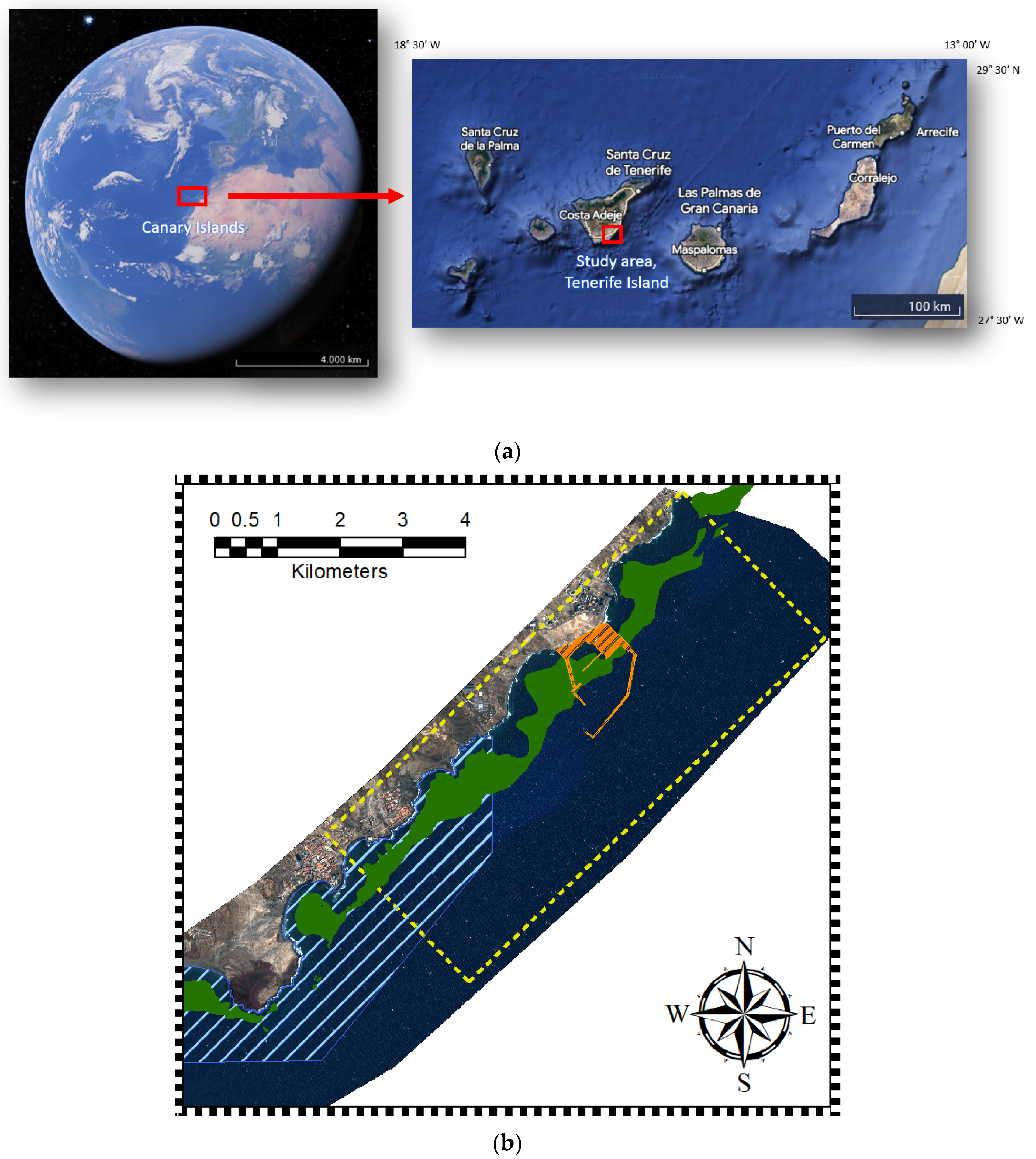
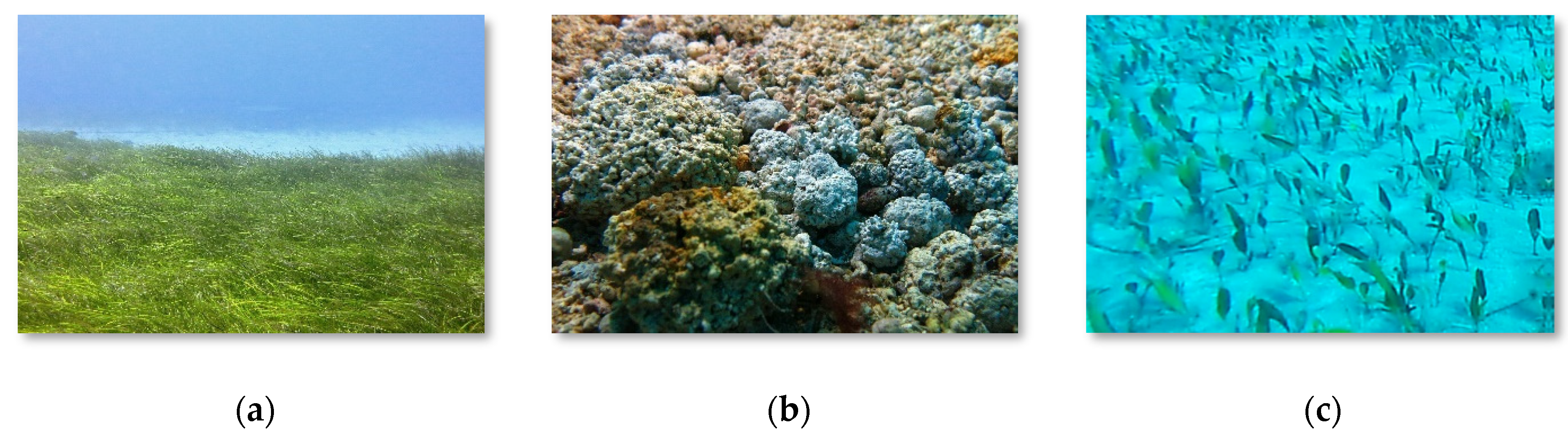
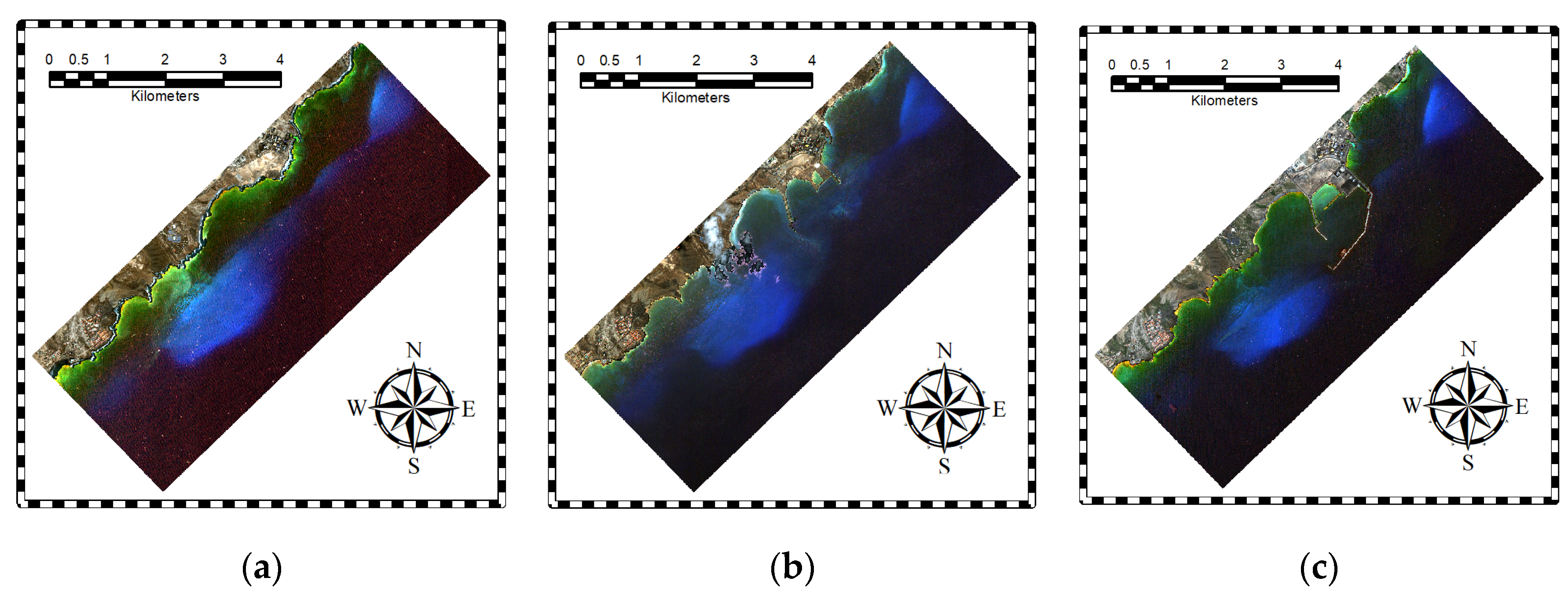
2.1. Study Area
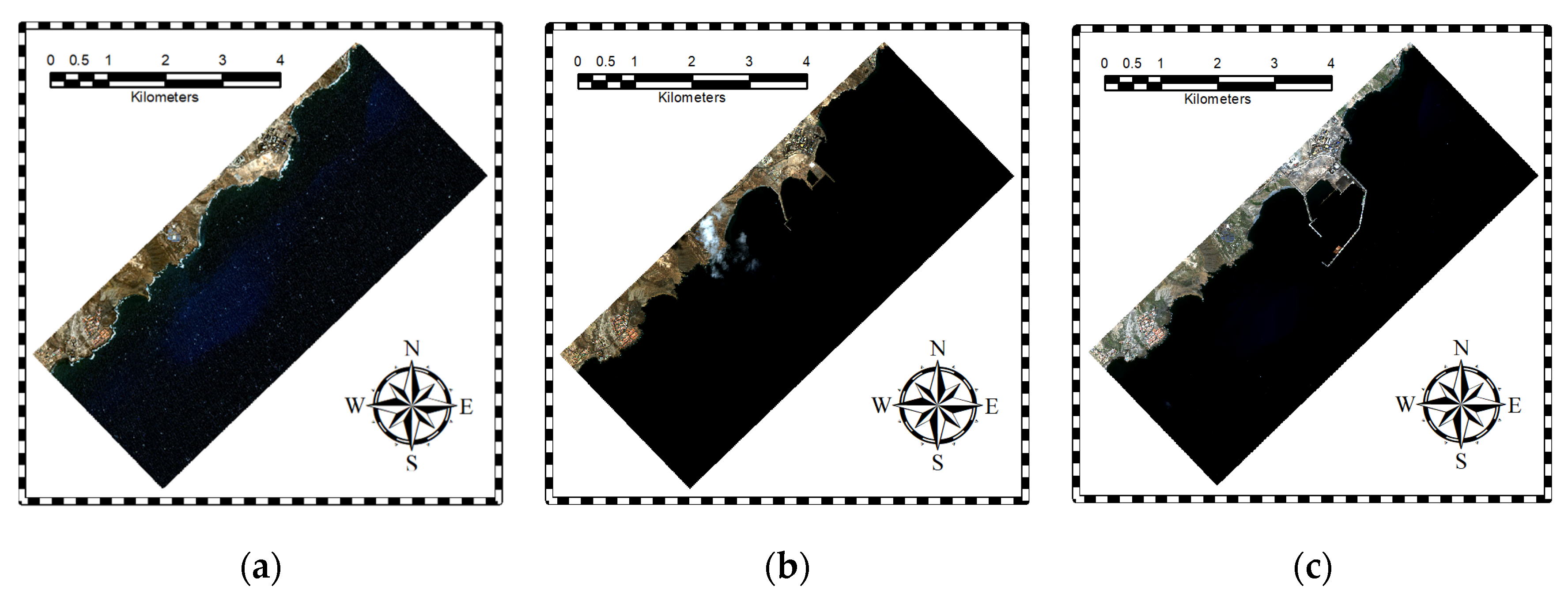
2.2. Data
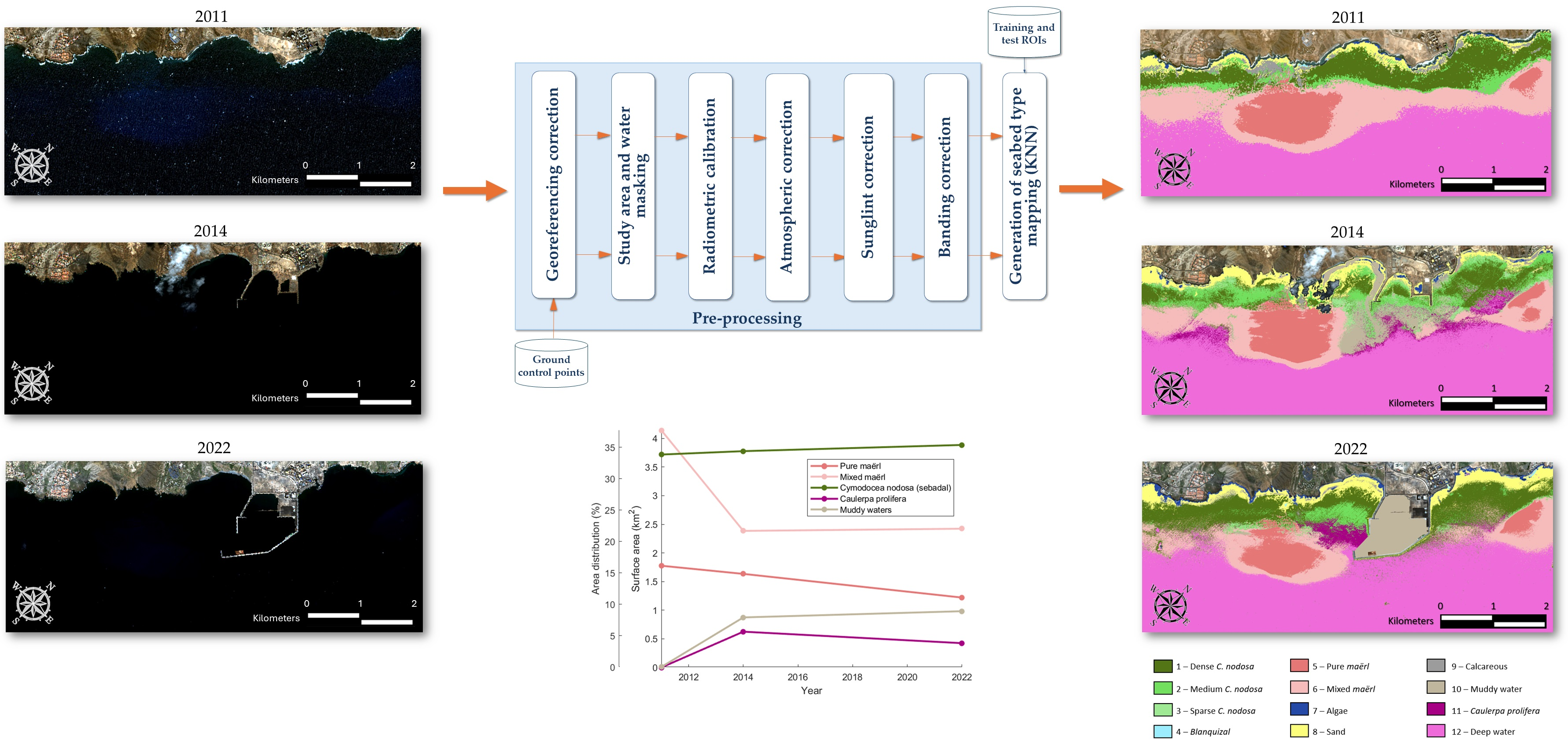
2.3. Imagery Processing
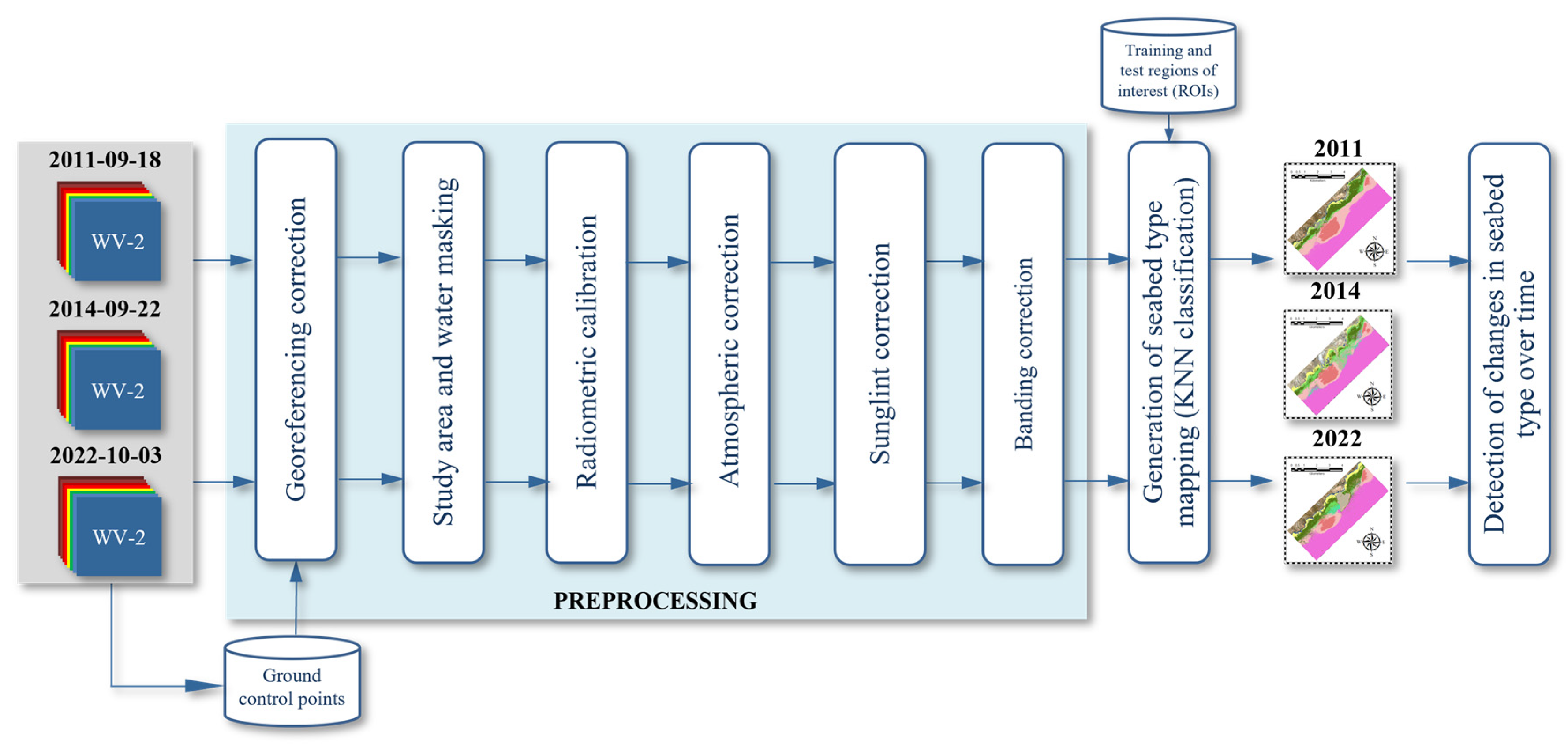
2.3.1. Pre-Processing
- Georeferencing correction
- Study area and water masking
- Radiometric correction
- Atmospheric correction
- Sunglint correction
- Banding correction
2.3.2. Classification
2.3.3. Detection of Changes in Seabed Type over Time
3. Results
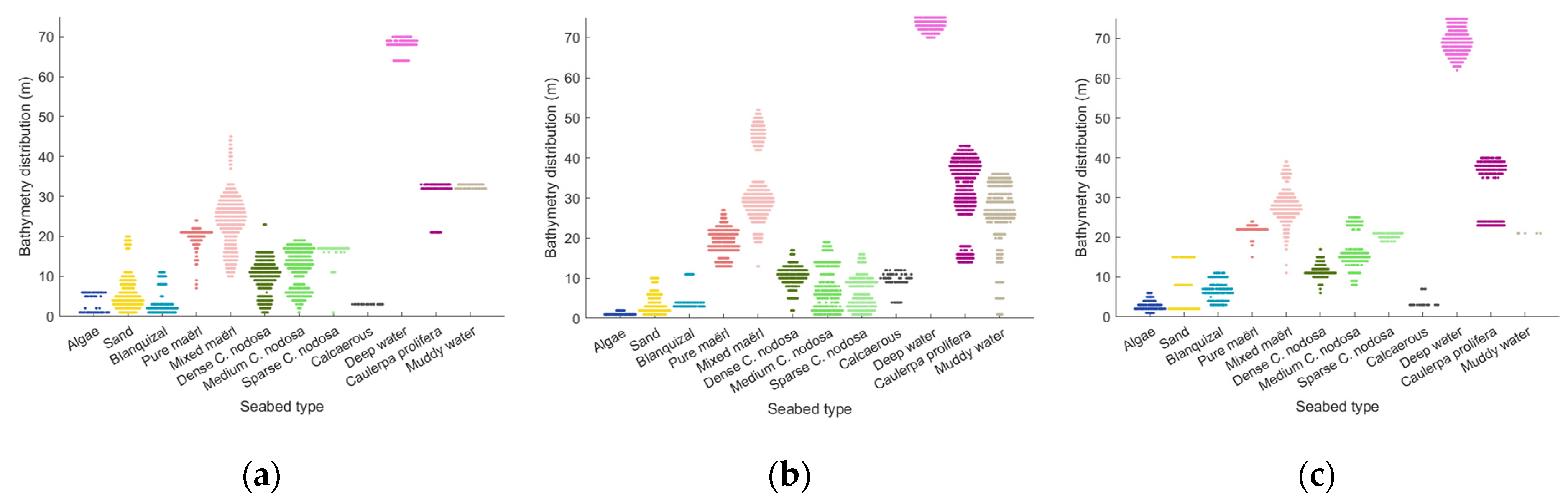
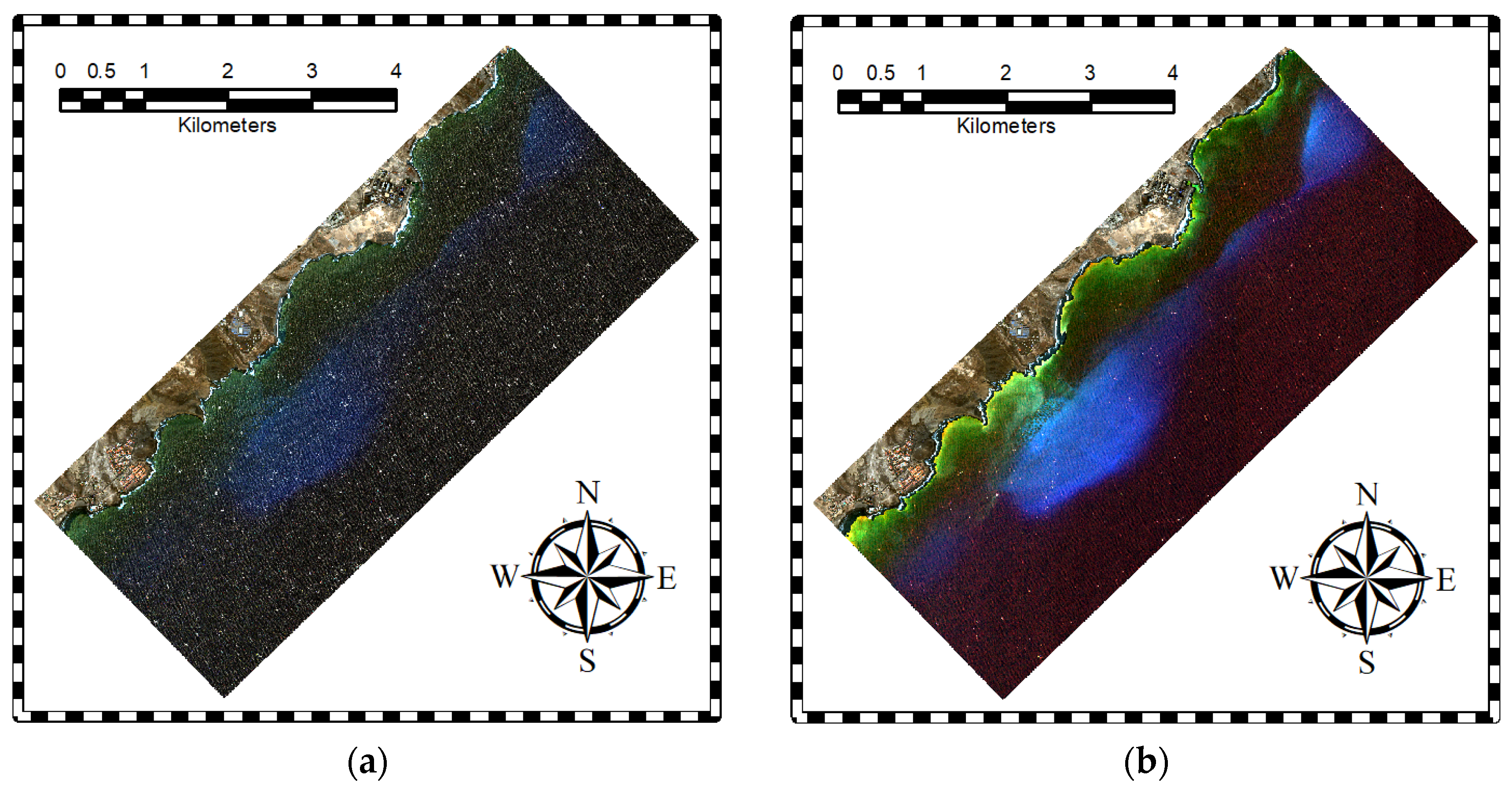
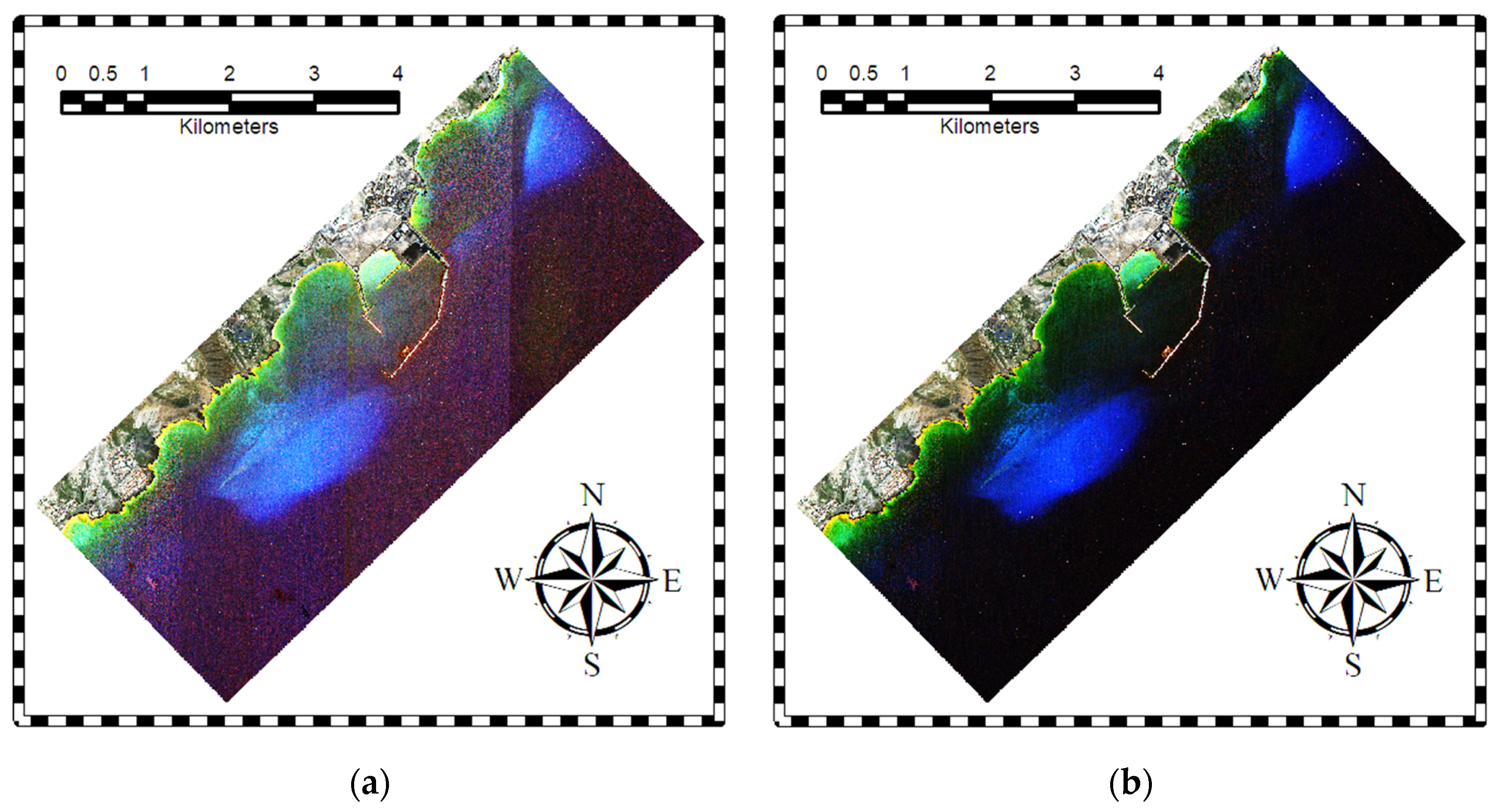
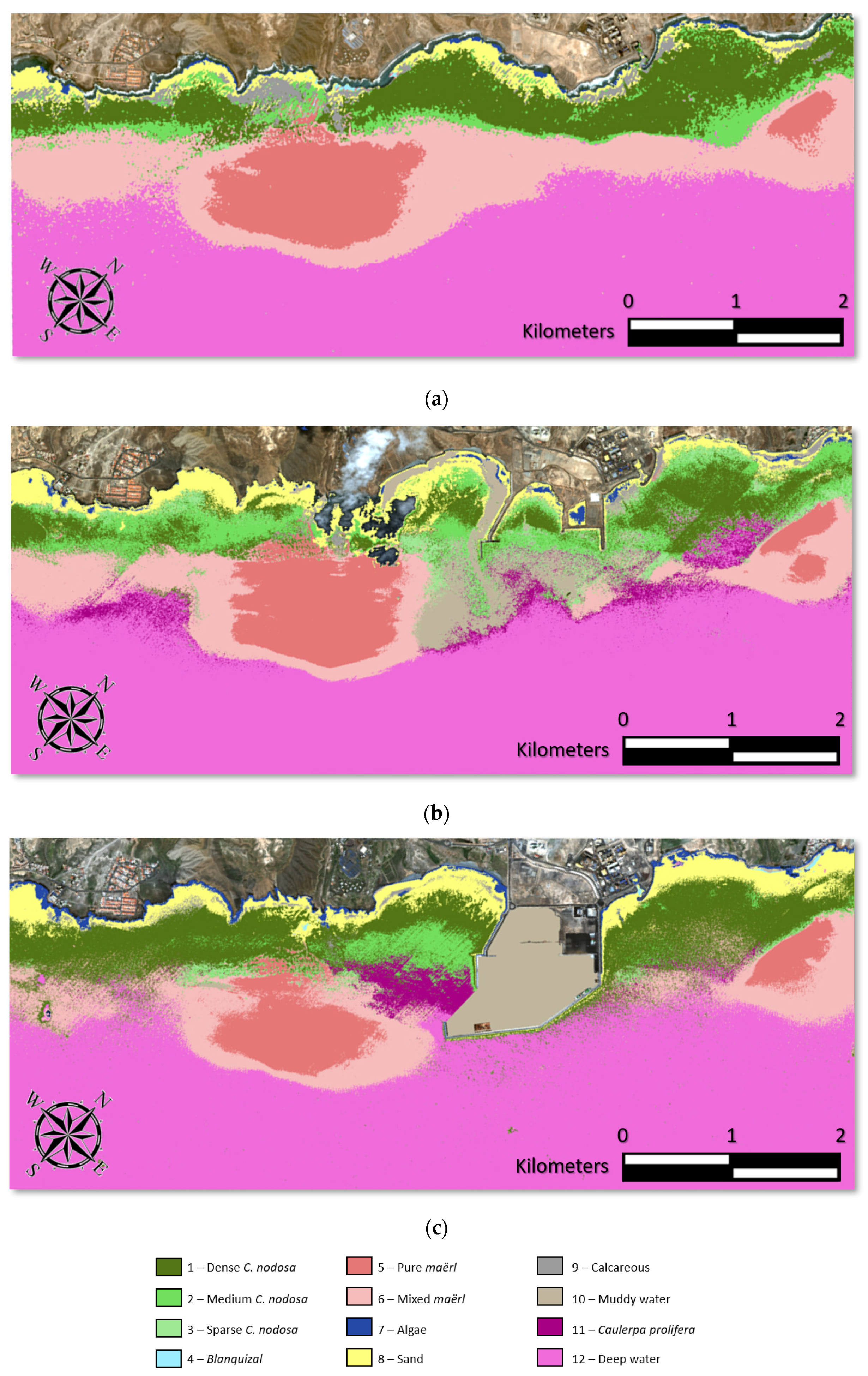
3.1. Seabed Maps
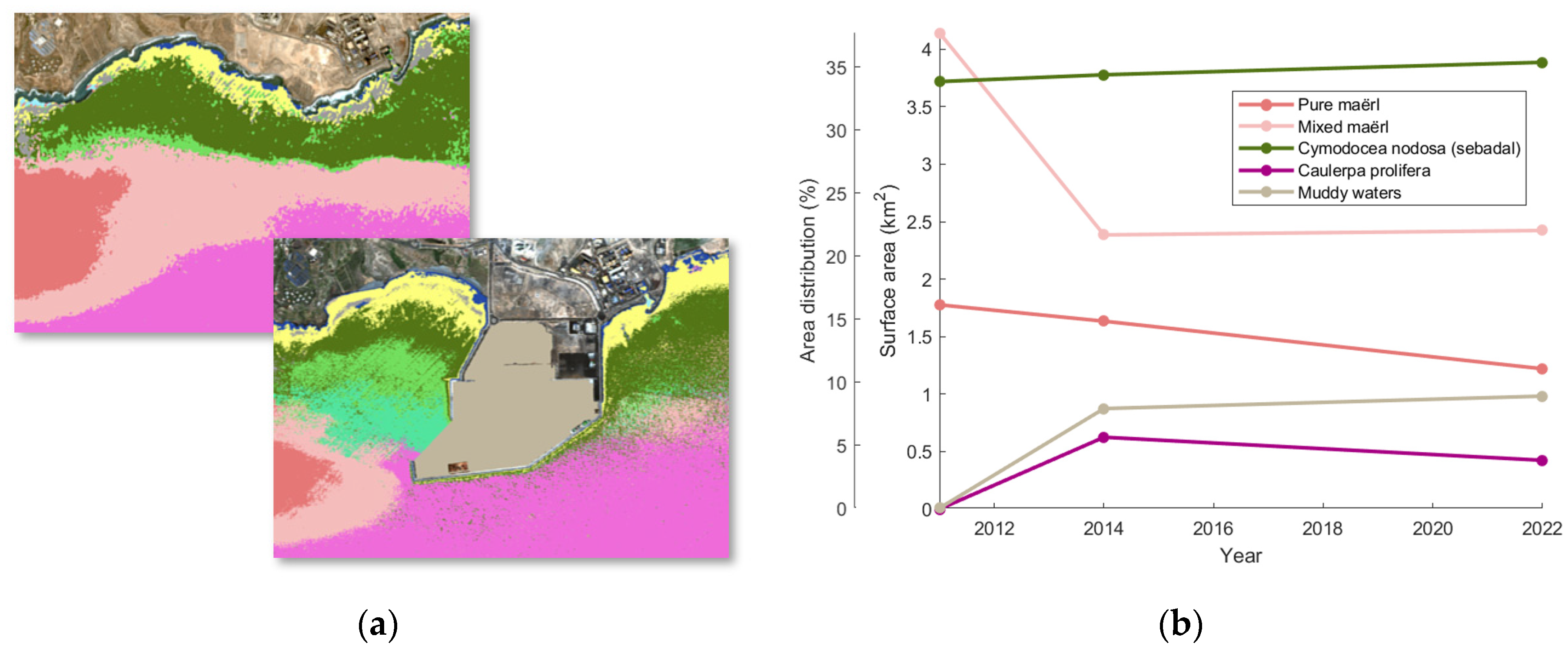
3.2. Temporal Evolution of the Seafloor
4. Discussion
5. Conclusions
Author Contributions
Funding
Data Availability Statement
Acknowledgments
Conflicts of Interest
References
- Green, E.P.; Short, F.T. World Atlas of Seagrasses; University of California Press: Berkeley, CA, USA, 2003. [Google Scholar]
- Hemminga, M.A.; Duarte, C.M. Seagrass Ecology; Cambridge University Press: Cambridge, UK, 2000. [Google Scholar]
- Björk, M.; Short, F.; Mcleod, E.; Beer, S. Managing Seagrasses for Resilience to Climate Change (No. 3); IUCN: Gland, Switzerland, 2008. [Google Scholar]
- Duarte, C.M.; Cebrián, J. The fate of marine autotrophic production. Limnol. Oceanogr. 1996, 41, 1758–1766. [Google Scholar] [CrossRef]
- Duarte, C.M. The future of seagrass meadows. Environ. Conserv. 2002, 29, 192–206. [Google Scholar] [CrossRef]
- Orth, R.J.; Curruthers, T.J.B.; Dennison, W.C.; Duarte, C.M.; Fourqurean, J.W.; Heck, K.L.; Hughes, A.R.; Kendrick, G.A.; Kenworthy, W.J.; Olyarnik, S.; et al. A global crisis for seagrass ecosystems. BioScience 2006, 56, 987–996. [Google Scholar] [CrossRef]
- Dunic, J.C.; Brown, C.J.; Connolly, R.M.; Turschwell, M.P.; Côté, I.M. Long-term declines and recovery of meadow area across the world’s seagrass bioregions. Glob. Chang. Biol. 2001, 27, 4096–4109. [Google Scholar] [CrossRef]
- Espino, F.; Tuya, F.; Blanch, I.; Haroun, R.J. Los Sebadales en Canarias. Oasis de Vida en los Fondos Arenosos; BIOGES, Universidad de Las Palmas de Gran Canaria: Las Palmas de Gran Canaria, Spain, 2008; 45p. [Google Scholar]
- Trenberth, K. Uncertainty in hurricanes and global warming. Science 2005, 308, 1753–1754. [Google Scholar] [CrossRef]
- Short, F.T.; Dennison, W.C.; Carruthers, T.J.B.; Waycott, M. Global seagrass distribution and diversity: A bioregional model. J. Exp. Mar. Biol. Ecol. 2007, 350, 3–20. [Google Scholar] [CrossRef]
- Overpeck, J.T.; Otto-Bliesner, B.L.; Miller, G.H.; Muhs, D.R.; Alley, R.B.; Kiehl, J.T. Paleoclimatic evidence for future ice-sheet instability and rapid sea-level rise. Science 2006, 311, 1747–1750. [Google Scholar] [CrossRef]
- Sunny, A.R. A review on effect of global climate change on seaweed and seagrass communities. Int. J. Fish. Aquat. Sci. 2017, 28, 8. [Google Scholar]
- Wiencke, C.; Bischof, K. Seaweed biology. Ecol. Stud. 2012, 219. [Google Scholar] [CrossRef]
- Harley, C.D.; Anderson, K.M.; Demes, K.W.; Jorve, J.P.; Kordas, R.L.; Coyle, T.A.; Graham, M.H. Effects of climate change on global seaweed communities. J. Phycol. 2012, 48, 1064–1078. [Google Scholar] [CrossRef]
- Short, F.T.; Burdick, D.M.; Kaldy, J.E. Mesocosm experiments quantify the effects of eutrophication on eelgrass, Zostera marina L. Limnol. Oceanogr. 1995, 40, 740–749. [Google Scholar] [CrossRef]
- Ruiz, J.M.; Guillén, J.E.; Ramos-Segura, A.; Otero, M.M. Atlas de las Praderas Marinas de España; Instituto Español de Oceanografía: Madrid, Spain, 2015. [Google Scholar]
- Horning, N.; Robinson, J.A.; Sterling, E.J.; Turner, W. Remote Sensing for Ecology and Conservation: A Handbook of Techniques; Oxford University Press: Oxford, UK, 2010. [Google Scholar]
- Purkis, S.J.; Klemas, V.V. Remote Sensing and Global Environmental Change; John Wiley & Sons: Hoboken, NJ, USA, 2011. [Google Scholar]
- Kenny, A.J.; Cato, I.; Desprez, M.; Fader, G.; Schüttenhelm, R.T.E.; Side, J. An overview of seabed-mapping technologies in the context of marine habitat classification. ICES J. Mar. Sci. 2003, 60, 411–418. [Google Scholar] [CrossRef]
- Marcello, J.; Eugenio, F.; Martín, J.; Marqués, F. Seabed mapping in coastal shallow waters using high resolution multispectral and hyperspectral imagery. Remote Sens. 2018, 10, 1208. [Google Scholar] [CrossRef]
- Veettil, B.K.; Ward, R.D.; Lima, M.D.A.C.; Stankovic, M.; Hoai, P.N.; Quang, N.X. Opportunities for seagrass research derived from remote sensing: A review of current methods. Ecol. Indic. 2020, 117, 106560. [Google Scholar] [CrossRef]
- Mederos-Barrera, A.; Marcello, J.; Eugenio, F.; Hernández, E. Seagrass mapping using high resolution multispectral satellite imagery: A comparison of water column correction models. Int. J. Appl. Earth Obs. Geoinf. 2022, 113, 102990. [Google Scholar] [CrossRef]
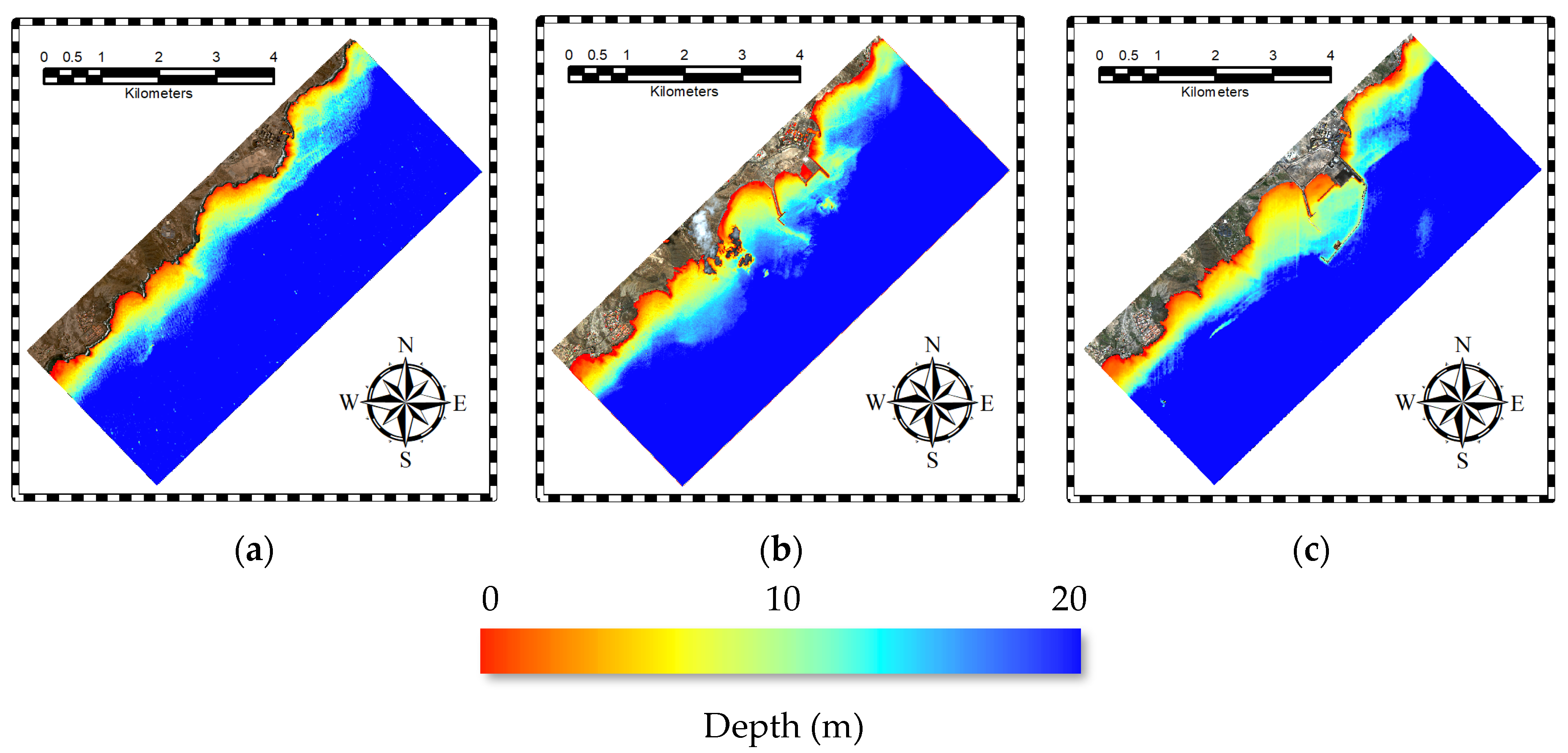
- Eugenio, F.; Marcello, J.; Mederos-Barrera, A.; Marqués, F. High Resolution Satellite Bathymetry Mapping: Regression and Machine Learning Based Approaches. IEEE Trans. Geosci. Remote Sens. 2022, 60, 5407614. [Google Scholar] [CrossRef]
- Blake, C.; Maggs, C.A. Comparative growth rates and internal banding periodicity of maërl species (Corallinales, Rhodophyta) from northern Europe. Phycologia 2003, 42, 606–612. [Google Scholar] [CrossRef]
- Barbera, C.; Bordehore, C.; Borg, J.A.; Glémarec, M.; Grall, J.; Hall-Spencer, J.M.; de la Huz, C.; Lanfranco, E.; Lastra, M.; Moore, P. Conservation and management of northeast Atlantic and Mediterranean maerl beds. Aquat. Conserv. Mar. Freshw. Ecosyst. 2003, 13, S65–S76. [Google Scholar] [CrossRef]
- Nelson, W.A. Calcified macroalgae—Critical to coastal ecosystems and vulnerable to change: A review. Mar. Freshw. Res. 2009, 60, 787–801. [Google Scholar] [CrossRef]
- Sathyendranath, S. Remote Sensing of Ocean Colour in Coastal, and Other Optically-Complex, Waters; International Ocean Colour Coordinating Group: Dartmouth, NS, Canada, 2000. [Google Scholar]
- McFeeters, S.K. The use of the Normalized Difference Water Index (NDWI) in the delineation of open water features. Int. J. Remote Sens. 1996, 17, 1425–1432. [Google Scholar] [CrossRef]
- Updike, T.; Comp, C. Radiometric Use of WorldView-2 Imagery; Technical Note; DigitalGlobe: Westminster, CO, USA, 2010; pp. 1–17. [Google Scholar]
- Labsch, H.; Handorf, D.; Dethloff, K.; Kurgansky, M.V. Atmospheric circulation regimes in a nonlinear quasi-geostrophic model. Adv. Meteorol. 2015, 629429. [Google Scholar] [CrossRef]
- Eugenio, F.; Marcello, J.; Martin, J. High-Resolution Maps of Bathymetry and Benthic Habitats in Shallow-Water Environments Using Multispectral Remote Sensing Imagery. IEEE Trans. Geosci. Remote Sens. 2015, 53, 3539–3549. [Google Scholar] [CrossRef]
- Eugenio, F.; Marcello, J.; Martin, J.; Rodríguez-Esparragón, D. Benthic Habitat Mapping Using Multispectral High-Resolution Imagery: Evaluation of Shallow Water Atmospheric Correction Techniques. Sensors 2017, 17, 2639. [Google Scholar] [CrossRef]
- Vermote, E.F.T.D.; Tanré, D.; Deuzé, J.L.; Herman, M.; Morcrette, J.J.; Kotchenova, S.Y. Second Simulation of a Satellite Signal in the Solar Spectrum-Vector (6SV); 6S User Guide Version; University of Maryland: Maryland, DC, USA, 2006; Volume 3, pp. 1–55. [Google Scholar]
- Kay, S.; Hedley, J.D.; Lavender, S. Sun glint correction of high and low spatial resolution images of aquatic scenes: A review of methods for visible and near-infrared wavelengths. Remote Sens. 2009, 1, 697–730. [Google Scholar] [CrossRef]
- Lyzenga, D.R.; Malinas, N.P.; Tanis, F.J. Multispectral bathymetry using a simple physically based algorithm. IEEE Trans. Geosci. Remote Sens. 2006, 44, 2251–2259. [Google Scholar] [CrossRef]
- Hedley, J.D.; Harborne, A.R.; Mumby, P.J. Simple and robust removal of sun glint for mapping shallow-water benthos. Int. J. Remote Sens. 2005, 26, 2107–2112. [Google Scholar] [CrossRef]
- Salehi, B.; Zhang, Y.; Zhong, M. Automatic moving vehicles information extraction from single-pass WorldView-2 imagery. IEEE J. Sel. Top. Appl. Earth Obs. Remote Sens. 2012, 5, 135–145. [Google Scholar] [CrossRef]
- Coffer, M.M.; Whitman, P.J.; Schaeffer, B.A.; Hill, V.; Zimmerman, R.C.; Salls, W.B.; Graybill, D.D. Vertical artifacts in high-resolution WorldView-2 and WorldView-3 satellite imagery of aquatic systems. Int. J. Remote Sens. 2022, 43, 1199–1225. [Google Scholar] [CrossRef] [PubMed]
- Mather, P.; Tso, B. Classification Methods for Remotely Sensed Data; CRC Press: Boca Raton, FL, USA, 2016. [Google Scholar]
- Sheykhmousa, M.; Mahdianpari, M.; Ghanbari, H.; Mohammadimanesh, F.; Ghamisi, P.; Homayouni, S. Support vector machine versus random forest for remote sensing image classification: A meta-analysis and systematic review. IEEE J. Sel. Top. Appl. Earth Obs. Remote Sens. 2020, 13, 6308–6325. [Google Scholar] [CrossRef]
- Chirici, G.; Mura, M.; McInerney, D.; Py, N.; Tomppo, E.O.; Waser, L.T.; Travaglini, D.; McRoberts, R.E. A meta-analysis and review of the literature on the k-Nearest Neighbors technique for forestry applications that use remotely sensed data. Remote Sens. Environ. 2016, 176, 282–294. [Google Scholar] [CrossRef]
- Maulik, U.; Chakraborty, D. Remote Sensing Image Classification: A survey of support-vector-machine-based advanced techniques. IEEE Geosci. Remote Sens. Mag. 2017, 5, 33–52. [Google Scholar] [CrossRef]
- Zhu, X.X.; Tuia, D.; Mou, L.; Xia, G.S.; Zhang, L.; Xu, F.; Fraundorfer, F. Deep learning in remote sensing: A comprehensive review and list of resources. IEEE Geosci. Remote Sens. Mag. 2017, 5, 8–36. [Google Scholar] [CrossRef]
- Yuan, Q.; Shen, H.; Li, T.; Li, Z.; Li, S.; Jiang, Y.; Xu, H.; Tan, W.; Yang, Q.; Wang, J.; et al. Deep learning in environmental remote sensing: Achievements and challenges. Remote Sens. Environ. 2020, 241, 111716. [Google Scholar] [CrossRef]
- Rukundo, O.; Cao, H. Nearest neighbor value interpolation. Int. J. Adv. Comput. Sci. Appl. 2012, 3, 4. [Google Scholar]
- Martin, S.; Clavier, J.; Chauvaud, L.; Thouzeau, G. Community metabolism in temperate maerl beds. I. Carbon and carbonate fluxes. Mar. Ecol. Prog. Ser. 2007, 335, 19–29. [Google Scholar] [CrossRef]
- Ceccherelli, G.; Cinelli, F. Short-term effects of nutrient enrichment of the sediment and interactions between the seagrass Cymodocea nodosa and the introduced green alga Caulerpa taxi- folia in the Mediterranean bay. J. Exp. Mar. Biol. Ecol. 1997, 217, 165–177. [Google Scholar] [CrossRef]
- Ceccherelli, G.; Sechi, N. Nutrient availability in the sediment and the reciprocal effects between the native seagrass Cymodocea nodosa and the introduced rhizophytic alga Caulerpa taxifolia. Hydrobiologia 2002, 474, 57–66. [Google Scholar] [CrossRef]
- Stumpf, R.P.; Holderied, K.; Sinclair, M. Determination of water depth with high-resolution satellite imagery over variable bottom types. Limnol. Oceanogr. 2003, 48, 547–556. [Google Scholar] [CrossRef]
- Gobierno de Canarias. Censo De Vertidos Desde Tierra Al Mar En Canarias: Emisario Submarino de La Batata—Ensenada Pelada (Code 02TFGR, ID 416); Gobierno de Canarias: Las Palmas de Gran Canaria, Spain, 2021; Available online: https://www.idecanarias.es/resources/Vertidos_2021/Fichas/Tenerife/416.pdf (accessed on 6 March 2022).
- Grupo Tragsa. Actualización del Censo de Vertidos Desde Tierra al mar en Canarias 2021: Memoria General Canarias; Gobierno de Canarias: Las Palmas de Gran Canaria, Spain, 2022; Available online: https://www.gobiernodecanarias.org/medioambiente/descargas/Aguas/Censo_vertidos_2021/01-MEMORIAS/Canarias.pdf (accessed on 6 March 2022).
- Pérez-Fernández, J. Contribución al Conocimiento del Efecto de Los Emisarios Submarinos y Los Diques Sobre Las Praderas Marinas de" Cymodocea Nodosa": Estudio del Emisario Submarino de la Playa de El Cochino y el Dique Del Puerto de Taliarte en Gran Canaria; Universidad de Las Palmas de Gran Canaria: Las Palmas de Gran Canaria, Spain, 2001. [Google Scholar]


| Date | Recall ↑ | Precision ↑ | F1 Score ↑ |
|---|---|---|---|
| 18 September 2011 | 76% | 85% | 80% |
| 22 September 2014 | 77% | 81% | 79% |
| 3 October 2022 | 76% | 80% | 77% |
| Predicted Class | |||||||||||||
|---|---|---|---|---|---|---|---|---|---|---|---|---|---|
| 1 | 2 | 3 | 4 | 5 | 6 | 7 | 8 | 9 | 10 | 11 | 12 | ||
| True Class | 1 | 78.5 | 17.1 | 1.9 | 2.5 | ||||||||
| 2 | 18.5 | 67.6 | 8.8 | 5.1 | |||||||||
| 3 | 3.5 | 3.8 | 65.2 | 24.0 | 3.5 | ||||||||
| 4 | 79.9 | 20.1 | |||||||||||
| 5 | 97.6 | 2.4 | |||||||||||
| 6 | 5.5 | 88.5 | 6.0 | ||||||||||
| 7 | 93.1 | 6.9 | |||||||||||
| 8 | 4.5 | 4.6 | 90.9 | ||||||||||
| 9 | 9.3 | 10.6 | 80.1 | ||||||||||
| 10 | 6.8 | 17.6 | 37.8 | 37.8 | |||||||||
| 11 | 28.5 | 24.7 | 46.8 | ||||||||||
| 12 | 2.6 | 6.8 | 90.6 | ||||||||||
| Predicted Class | |||||||||||||
|---|---|---|---|---|---|---|---|---|---|---|---|---|---|
| 1 | 2 | 3 | 4 | 5 | 6 | 7 | 8 | 9 | 10 | 11 | 12 | ||
| True Class | 1 | 75.6 | 12.8 | 6.7 | 4.9 | ||||||||
| 2 | 14.7 | 62.1 | 10.7 | 5.8 | 6.7 | ||||||||
| 3 | 16.3 | 16.7 | 53.7 | 7.1 | 6.2 | ||||||||
| 4 | 72.2 | 2.2 | 16.1 | 9.5 | |||||||||
| 5 | 96.6 | 2.7 | 0.7 | ||||||||||
| 6 | 5.9 | 87.3 | 4.2 | 2.6 | |||||||||
| 7 | 1.5 | 84.1 | 14.4 | ||||||||||
| 8 | 3.6 | 2.6 | 4.0 | 4.4 | 85.4 | ||||||||
| 9 | 28.4 | 71.6 | |||||||||||
| 10 | 2.9 | 5.9 | 86.9 | 4.3 | |||||||||
| 11 | 3.8 | 3.0 | 11.8 | 9.1 | 55.0 | 17.3 | |||||||
| 12 | 0.7 | 2.5 | 96.8 | ||||||||||
| Predicted Class | |||||||||||||
|---|---|---|---|---|---|---|---|---|---|---|---|---|---|
| 1 | 2 | 3 | 4 | 5 | 6 | 7 | 8 | 9 | 10 | 11 | 12 | ||
| True Class | 1 | 78.1 | 8.7 | 4.4 | 3.3 | 5.5 | |||||||
| 2 | 33.4 | 50.8 | 7.3 | 4.5 | 4.0 | ||||||||
| 3 | 16.3 | 11.9 | 38.3 | 24.4 | 9.1 | ||||||||
| 4 | 23.2 | 5.8 | 56.6 | 14.4 | |||||||||
| 5 | 92.1 | 7.9 | |||||||||||
| 6 | 7.0 | 78.5 | 7.8 | 6.7 | |||||||||
| 7 | 2.5 | 2.3 | 95.2 | ||||||||||
| 8 | 3.5 | 1.2 | 95.3 | ||||||||||
| 9 | 13.4 | 86.6 | |||||||||||
| 10 | 6.5 | 6.6 | 86.9 | ||||||||||
| 11 | 2.6 | 2.5 | 27.5 | 52.3 | 15.1 | ||||||||
| 12 | 2.6 | 1.0 | 96.4 | ||||||||||
Disclaimer/Publisher’s Note: The statements, opinions and data contained in all publications are solely those of the individual author(s) and contributor(s) and not of MDPI and/or the editor(s). MDPI and/or the editor(s) disclaim responsibility for any injury to people or property resulting from any ideas, methods, instructions or products referred to in the content. |
© 2024 by the authors. Licensee MDPI, Basel, Switzerland. This article is an open access article distributed under the terms and conditions of the Creative Commons Attribution (CC BY) license (https://creativecommons.org/licenses/by/4.0/).
Share and Cite
Mederos-Barrera, A.; Sevilla, J.; Marcello, J.; Espinosa, J.M.; Eugenio, F. Effects of the Construction of Granadilla Industrial Port in Seagrass and Seaweed Habitats Using Very-High-Resolution Multispectral Satellite Imagery. Remote Sens. 2024, 16, 945. https://doi.org/10.3390/rs16060945
Mederos-Barrera A, Sevilla J, Marcello J, Espinosa JM, Eugenio F. Effects of the Construction of Granadilla Industrial Port in Seagrass and Seaweed Habitats Using Very-High-Resolution Multispectral Satellite Imagery. Remote Sensing. 2024; 16(6):945. https://doi.org/10.3390/rs16060945
Chicago/Turabian StyleMederos-Barrera, Antonio, José Sevilla, Javier Marcello, José María Espinosa, and Francisco Eugenio. 2024. "Effects of the Construction of Granadilla Industrial Port in Seagrass and Seaweed Habitats Using Very-High-Resolution Multispectral Satellite Imagery" Remote Sensing 16, no. 6: 945. https://doi.org/10.3390/rs16060945