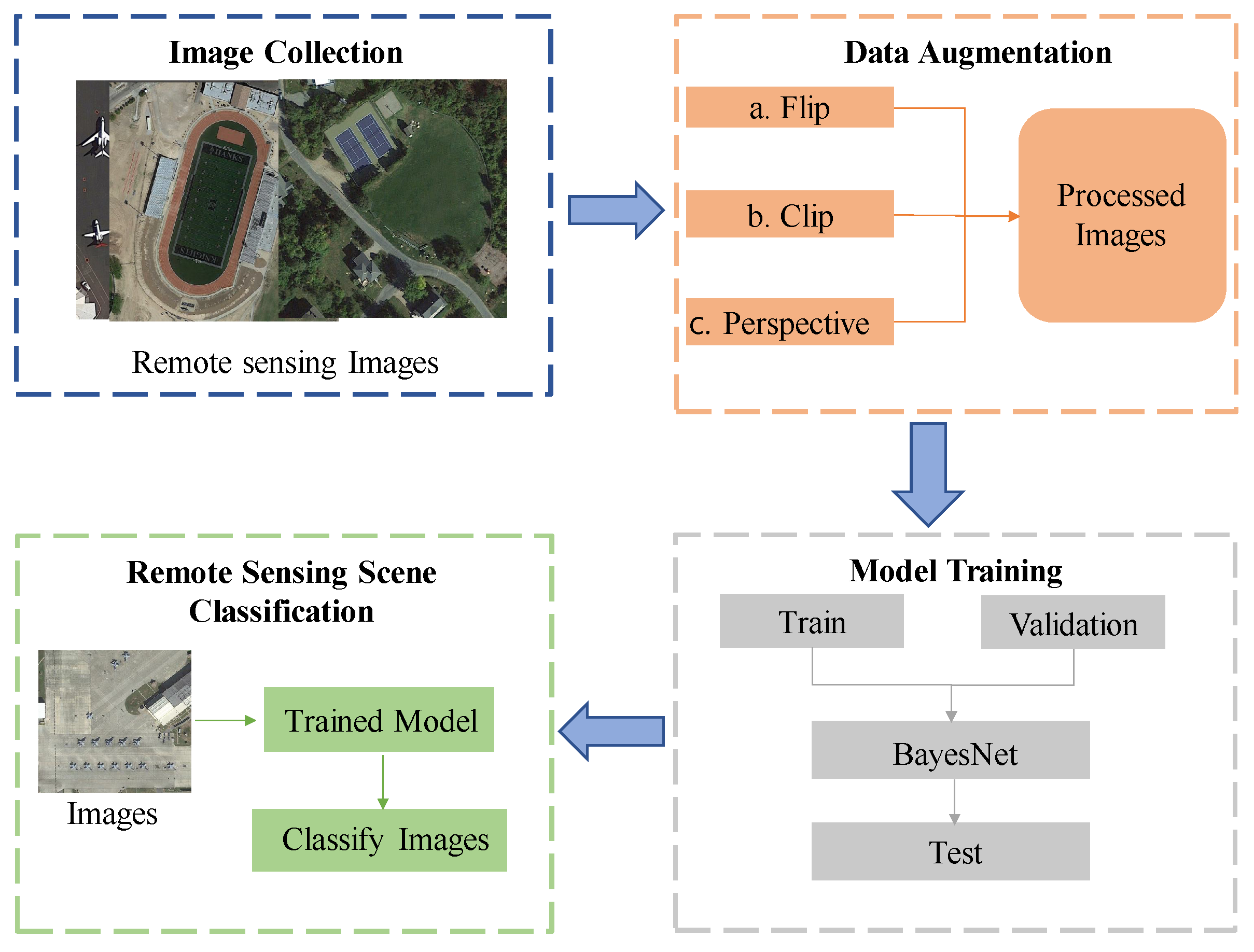
Article

BayesNet: Enhancing UAV-Based Remote Sensing Scene Understanding with Quantifiable Uncertainties

1
Department of Intelligent Mechatronics Engineering, Sejong University, Seoul 05006, Republic of Korea
2
Department of Computer Science and Engineering, Sejong University, Seoul 05006, Republic of Korea
3
Ningbo Institute of Materials Technology and Engineering, Chinese Academy of Sciences, Ningbo 315201, China
4
Department of Information and Communication Engineering and Convergence Engineering for Intelligent Drone, Sejong University, Seoul 05006, Republic of Korea
*
Author to whom correspondence should be addressed.
These authors contributed equally to this work.
Remote Sens. 2024, 16(5), 925; https://doi.org/10.3390/rs16050925
Submission received: 21 January 2024 / Revised: 26 February 2024 / Accepted: 1 March 2024 / Published: 6 March 2024
(This article belongs to the Section AI Remote Sensing)

Abstract

:
Remote sensing stands as a fundamental technique in contemporary environmental monitoring, facilitating extensive data collection and offering invaluable insights into the dynamic nature of the Earth’s surface. The advent of deep learning, particularly convolutional neural networks (CNNs), has further revolutionized this domain by enhancing scene understanding. However, despite the advancements, traditional CNN methodologies face challenges such as overfitting in imbalanced datasets and a lack of precise uncertainty quantification, crucial for extracting meaningful insights and enhancing the precision of remote sensing techniques. Addressing these critical issues, this study introduces BayesNet, a Bayesian neural network (BNN)-driven CNN model designed to normalize and estimate uncertainties, particularly aleatoric and epistemic, in remote sensing datasets. BayesNet integrates a novel channel–spatial attention module to refine feature extraction processes in remote sensing imagery, thereby ensuring a robust analysis of complex scenes. BayesNet was trained on four widely recognized unmanned aerial vehicle (UAV)-based remote sensing datasets, UCM21, RSSCN7, AID, and NWPU, and demonstrated good performance, achieving accuracies of 99.99%, 97.30%, 97.57%, and 95.44%, respectively. Notably, it has showcased superior performance over existing models in the AID, NWPU, and UCM21 datasets, with enhancements of 0.03%, 0.54%, and 0.23%, respectively. This improvement is significant in the context of complex scene classification of remote sensing images, where even slight improvements mark substantial progress against complex and highly optimized benchmarks. Moreover, a self-prepared remote sensing testing dataset is also introduced to test BayesNet against unseen data, and it achieved an accuracy of 96.39%, which showcases the effectiveness of the BayesNet in scene classification tasks.

1. Introduction

Remote sensing imaging technology has advanced significantly over the years, enabling satellites and unmanned aerial vehicles (UAVs) equipped with sophisticated sensors to capture high-resolution images. These images are comprehensive, of high quality, and provide an excellent platform for object recognition and scene categorization. Remote sensing methods offer a range of techniques for presenting information about the Earth’s surface, including classification, detection, and scene understanding, without the need for physical interaction.
However, remote sensing objects can be challenging to discern due to their varying sizes and locations [1,2,3]. To address this challenge, annotated aerial imagery is utilized to construct modern machine learning and deep learning models. Moreover, the conventional classification of remote sensing objects is often a time-consuming process, requiring experts to examine and interpret each image individually [4,5].
To expedite this process, researchers are working on developing deep learning models to understand remote sensing scenes using classification models such as the convolutional neural network (CNN). Automatic feature extraction plays a crucial role in rapidly extracting essential information from the images, which saves processing time [6,7].
CNNs provide reliable and efficient tools for automatically predicting higher-level characteristics from input data. Hu et al. demonstrated the superiority of CNN-based strategies over classic machine learning algorithms in classification tasks using hyperspectral imagery [8]. This finding is crucial as it underlines the evolving trend toward more sophisticated, data-driven approaches in remote sensing, a trend that our study builds upon by exploring Bayesian methods. Similarly, Grana et al. compared deep learning algorithms and Monte Carlo approaches for classifying facies from seismic data [9]. This comparison is pivotal in highlighting the strengths and weaknesses of various computational approaches, informing our choice of methodology. However, they only consider machine learning methods which do not provide the measurement of the uncertainty.
Zhang et al. [10] employed deep learning to classify seismic facies within stratigraphic sequences. Their work contributes to the broader understanding of stratigraphic sequence classification but also highlights a limitation in addressing the complex patterns of seismic data, an aspect our study aims to tackle through improved feature extraction techniques. Li et al. introduced a unique pixel-pair technique for image classification [11], offering a novel perspective on spatial relationships in imagery. Their approach, though innovative, encounters limitations in processing efficiency, a gap that our study addresses by implementing a deep learning method. Zhao et al. proposed a spectral-spatial feature-based CNN classification framework [12]. Their work is significant for incorporating both spectral and spatial features, yet it underscores the challenge of integrating these features without significant computational overhead, an issue our research seeks to ameliorate.
Neeta and Saroj presented a semi-supervised classification model using neural networks [13]. However, their technique’s reliance on semi-supervised learning highlights a need for more robust fully supervised methods, especially in scenarios with limited labeled data, a challenge that our study addresses. Saroj proposed a deep auto-encoder neural network architecture [14] with a focus on automating feature extraction and enhancing generalization capability; while this method is innovative in leveraging neighborhood rough sets, it do not fully capture the complex, multi-dimensional nature of remote sensing data, an area where our research contributes by implementing a more comprehensive feature analysis framework. Wu and Guo’s introduction of a robust interval type-2 fuzzy clustering method [15] represents a significant stride in handling uncertainties in remote sensing image classification. Their approach to address category density and object spectra uncertainties is enlightening. Nevertheless, the method’s complexity in handling overlapping categories exposes the need for a more robust yet equally effective approach, which our study aims to provide.
While traditional CNNs outperform conventional machine learning approaches regarding classification, their deterministic parameters do not allow for uncertainty calculation. Additionally, deterministic CNN-based predictions may provide inaccurate classification labeling, leading to unintended consequences if not accompanied by some measure of confidence. To address these issues, various methods have been developed to examine uncertainty in classification models. One of the most effective uncertainty estimation approaches is the Bayesian CNN model.
The Bayesian CNN is a probabilistic deep learning approach that quantifies uncertainty by utilizing stochastic weights and biases, as opposed to the deterministic counterparts in traditional CNNs. This stochastic parameterization allows the Bayesian CNN to capture data variability and calculate uncertainty in its predictions, resembling standard backpropagation. Furthermore, regularization of weights through variational free energy minimization is possible, similar to dropout regularization. Shridhar et al. introduced this technique known as “Bayes via backprop”, which has demonstrated superior performance, including improved uncertainty measures and normalization, compared to traditional CNNs [16,17]. Kendall et al. proposed a Bayesian deep learning paradigm that addresses aleatoric and epistemic uncertainty [18], leading to a 1 to 3% performance boost over deterministic models, with the Monte Carlo dropout method by Gal et al. [19]. The growing popularity of Bayesian CNNs is attributed to their ability to incorporate uncertainty into predictions, which is crucial for applications like remote sensing data analysis [20,21]. This uncertainty assessment contributes to enhancing data quality, preventing overfitting, and ensuring precise models, though their accuracy is not yet on par with state-of-the-art models, especially in remote sensing scene classification.
This study introduces BayesNet as a means to enhance classification performance across four remote sensing datasets. The modified RegNet deep learning model to further improve performance and propose a novel Channel–Spatial Attention module (CSAM) to enhance feature extraction. The performance of the proposed model is evaluated using standard multiclass performance evaluation metrics, and aleatoric and epistemic uncertainty measures are calculated to infer the uncertainty caused by the model and dataset. A test dataset from a drone and publicly available images are utilized to test our proposed BayesNet. The main contributions of this paper can be summarized as follows:
  • A CNN-based remote sensing scene understanding method called BayesNet is proposed to improve the performance of the classification of four state-of-the-art datasets. To this end, this is the first time Bayesian CNN, specifically Bayes by backpropagation with variational inference, has been used in remote sensing applications. The previous Bayesian methods were only implemented to process hyperspectral remote sensing images.
  • The standard convolution layers are then replaced with the Bayes by backpropagation layers to bayesify the neural network.
  • A novel Channel–Spatial Attention module is proposed to improve the feature extraction of the proposed model.
  • BayesNet shows very good performance compared to other conventional CNN models. Moreover, the epistemic and aleatoric uncertainty is calculated using the proposed model, which can further improve the robustness of BayesNet in complex scene classification tasks.

2. Preliminaries

This section presented the background of the core Bayesian CNN models: the Bayesian neural network and its uncertainty quantification method.

2.1. Bayesian Neural Network

Conventional neural networks treat weights as fixed, rather than random, variables, operating under the assumption that the precise values of these weights are indeterminable and that data should be approached as a probabilistic process. Bayesian neural networks, on the other hand, infer the unknown weights of the model using data that are already known or observed [22]. Utilizing Bayes’ Theorem, it is possible to assign a probability distribution to these weights based on the likelihood of observed data, leading to the determination of the posterior distribution of parameters. This approach allows for the specification of a joint probability distribution that reflects the prior knowledge incorporated into the neural networks, which can be defined as follows,
P ( w | d ) = P ( d | w ) P ( w ) P ( d ) ,
where P ( w | d ) is the posterior probability of the weights (w) given the data (d), P ( d | w ) is the likelihood of the data given the weights, and P ( w ) is the prior distribution of the weights.
The likelihood of a given dataset in a Bayesian neural network (BNN) can be defined as follows.
P ( d | w ) = n = 1 N P y n | w , x n ,
where N represents the individual term of a dataset, y n represents the training data label, and x n represents the training data.
We can define a function y = f ( x ) to model the relationship between inputs { x 1 , , x N } and their respective outputs { y 1 , , y N }. By applying Bayesian inference, we can establish a prior probability distribution P ( f ) over potential functions, reflecting our initial understanding of which functions might explain our data. To update our beliefs based on observed data, we compute the posterior distribution P f | X , Y using Bayes’ theorem, enabling the prediction of outcomes for new input x * by considering all possible functions f as follows:
P y * | x * , X , Y = P y * | f * P f * | x * , X , Y d f * , = P y * | f * P y * | f * , w P w | x * , X , Y d f * d w ,
where P y * | x * , X , Y is the predictive distribution. The predictions about any given set of values can be estimated using this posterior distribution. Predictions are expressed as a probability distribution with regard to the likelihood function,
E q P d y * | x * = q θ ( w | d ) P w ( y | X ) d w ,
where q θ ( w | d ) is the variational posterior distribution of the weights, and P w ( y | X ) is the posterior of the weights for a given dataset.

2.2. Bayes by Backpropagation

Bayes by backprop utilizes variational inference to learn about the posterior distribution of weights in a neural network, represented as w q θ ( w | d ) , where q θ ( w | d ) is a variational posterior distribution of the weights given the data d, and θ is the parameter defining this distribution. The goal is to find the optimal parameters, θ o p t , that minimize the KL divergence between the variational posterior distribution q θ ( w | d ) and the true posterior distribution P ( w | d ) . This divergence measures the difference between the two distributions, guiding us towards a more accurate approximation of the true posterior. The optimization problem can be expressed as follows:
θ o p t = arg min θ K L q θ ( w | d ) P ( w | d ) = arg min θ K L q θ ( w | d ) P ( w ) E q ( w | θ ) [ log P ( d | w ) ] + log P ( d ) ,
where
K L q θ ( w | d ) | | P ( w ) = q θ ( w | d ) log q θ ( w | d ) P ( w ) d w .
The KL divergence, K L [ q θ ( w | d ) | | P ( w ) ] , is an integral that compares the variational posterior distribution q θ ( w | d ) to the prior P ( w ) , acting as a complexity cost. The expectation E q ( w | d ) [ log P ( d | w ) ] is the likelihood cost, indicating how well the weights explain the observed data d, without needing to consider log P ( d ) in optimization as it is constant.
Given the intractability of computing KL divergence directly, we can use a stochastic approach [16] by sampling weights from the variational posterior distribution q θ ( w | d )
F ( d , θ ) i = 1 n log q θ w ( i ) | d log P w ( i ) log P d | w ( i ) ,
where w ( i ) is the weights sampled from q θ ( w | d ) , and n is the number of samples drawn. It balances the model’s fit to the data (through the likelihood term) against the complexity of the model (through the prior term), optimizing the parameters θ to achieve a model that not only fits the data well but also incorporates uncertainty effectively.

2.3. Uncertainty Estimation

Uncertainty estimations are becoming very important for life-critical applications such as autonomous driving, remote sensing imagery, medical images, etc. Bayesian deep learning provides methods to estimate a model’s and dataset’s uncertainty. Uncertainty estimations can be divided into epistemic uncertainty and aleatoric uncertainty. Both uncertainties account for the variance of the probability distribution over the weights. Aleatoric uncertainty quantifies the noise that accompanies the data. This sort of uncertainty is introduced by the data collection technique, such as measurement noise or mobility noise that is consistent throughout the dataset. This cannot be minimized by collecting more data. On the other side, epistemic uncertainty is a measure of model-induced uncertainty. Epistemic uncertainty can also be reduced by providing more good data to the model.
The main object of using BayesNet for remote sensing scene classification is to estimate predictive distribution P d ( y * | x * ) which represents the probability of class, y * , given a new input, x * . The relevant equation can be expressed as follows:
P d ( y * | x * ) = P w ( y * | x * ) P d ( w ) d w .
It sums over all possible weights w, weighted by their probability given the dataset d. In our scenario, we approximate the posterior distribution of weights using Gaussian variational posterior distribution q θ ( w | d ) N w | μ , σ 2 . The parameter θ = { μ , σ } is learned from the dataset d. The predictive distribution is then reformulated as below;
P d ( y * | x * ) = C a t ( y * | f w ( x * ) ) N ( w | μ , σ 2 ) d w .
Due to the integral complexity, we can estimate it by sampling from variational posterior q θ ( w | d ) as follows:
E q P d y * | x * = q θ ( w | d ) P w ( y | x ) d w 1 T t = 1 T P w t y * | x * ,
where p w t y * | x * is the prediction of the model for the t-th weight sample. We then estimate the predictive variance of these predictions across different weight samples which can be represented as
Var q P y * | x * = E q y y T E q [ y ] E q [ y ] T .
Var q P y * | x * estimates the spread of the predictions and thus the uncertainty of the model’s output. Therefore, a high variance indicates a wide spread of predictions which lead to higher uncertainty. These variances can be further decomposed into two uncertainties such as aleatoric and epistemic. The aleatoric uncertainty represents the uncertainty in the data such as noise, which can be represented as
Aleatoric = 1 T t = 1 T diag p ^ t p ^ t p ^ t T
On the other hand, epistemic uncertainty reflects the uncertainty in the model’s parameters which can be from limited dataset or model complexity. It can be represented as follows.
Epistemic = 1 T t = 1 T p ^ t p ¯ p ^ t p ¯ T

3. BayesNet for Remote Sensing

Figure 1 presents an overview of our proposed approach for classification and uncertainty estimation using BayesNet. The remote sensing data is divided into training, validation, and testing sets. To improve the quality of the data, a data augmentation method was applied. The augmented data is then used to train and validate the model, resulting in a classified output sample. The aleatoric and epistemic uncertainty using softplus normalization was used to estimate uncertainty. This method provides a measure of the model’s reliability by estimating the uncertainty caused by the data and the model itself. Our approach enables the development of more accurate and reliable models for remote sensing data analysis, with the ability to quantify uncertainty to support decision-making in critical applications

3.1. Dataset Acquisition

Four remote sensing datasets are used to train our proposed model. These datasets include UCM21 [23], RSSCN7 [24], AID [25], and NWPU45 [26]. A detailed description of the implemented dataset can be seen in Table 1.

3.2. Data Augmentation

The datasets used in this study are divided into training and testing sets based on the author’s instructions. Specifically, the UCM21 [23], RSSCN7 [24], AID [25], and NWPU45 [26] datasets are split into training–testing ratios of 80:20, 50:50, 50:50, and 50:50, respectively. Data augmentation methods such as flip, clip, and perspective are employed to enhance the quantity and variety of samples within a dataset. These techniques not only broaden the scope of the dataset but also act as a form of regularization, aiding in the reduction of overfitting when training models are based on deep learning for classification purposes.

3.3. BayesNet Model

Figure 2 shows the overall architecture of the BayeNet model, which comprises three parts: stem, body, and block. The body consists of four stages, and each stage consists of i blocks, with each block containing several convolution layers and an attention network.
The structure of each block includes Bayes by backprop convolution layers (BBConv) and a Channel–Spatial Attention module (CSAM) for efficient feature extraction. The original block is modified by introducing BBConv and a CSAM module. An additional BBConv is added prior to implementing the Softplus activation function. The input is first passed through a 1 × 1 BBConv, followed by group 3 × 3 BBConv. The output is then passed through another two 1 × 1 BBConv. The residual layer is then implemented to add all relevant features before the Softplus activation function is applied for further processing.
Overall, the BayeNet model is designed to extract features from remote sensing images effectively by incorporating Bayes by backprop convolution layers and a CSAM attention module into the structure. This modification enhances the model’s ability to recognize small images with intricate backgrounds, making it a promising solution for effective feature extraction in remote sensing applications.
Figure 3 introduces the Channel–Spatial Attention Module (CSAM), a novel addition to each block of our model, comprising the Channel Attention Block and the Spatial Attention Block, while foundational models like the Squeeze-and-Excitation (SE) block [27], Frequency Channel Attention Networks (FcaNet) [28], and the Convolution Block Attention Module (CBAM) [29] have significantly influenced CNN architectures by focusing on critical input data areas. However, CSAM is designed to solve the intricate issues of remote sensing image scene understanding, addressing limitations of previous models by simultaneously extracting attention features from both channel and spatial dimensions. This concurrent extraction process ensures a balanced feature representation, avoiding the potential bias of one dimension overshadowing the other. As illustrated in Figure 4, the architectural distinction of CSAM from SE and CBAM is evident, providing an unbiased, comprehensive feature representation that significantly surpasses the traditional, dimensionally constrained approaches.
Unlike previous methods, CSAM uniquely incorporates the Discrete Fourier Transform (DFT) within its attention mechanisms, allowing for a transition of input feature maps from the spatial to the frequency domain. This integration not only preserves crucial positional data but also enhances the model’s ability to interpret complex remote sensing imagery by considering both low and high-frequency components of feature maps. The inclusion of high-frequency details, often overlooked in conventional methods, is particularly pivotal in discerning subtle, yet critical aspects of remote sensing scenes. As depicted in Figure 4, CSAM’s innovative approach to feature extraction and its comprehensive frequency component analysis underscore its superiority over existing models like SE, CBAM, and FcaNet, especially in the field of remote sensing image scene understanding. This highlights the novelty and potential of CSAM in the application of attention mechanisms for remote sensing image processing.
The CSAM module consists of two parts including the Channel and Spatial Attention block. The Channel Attention block focuses on the channel-wise properties of remote sensing images. The input of the Channel Attention block first undergoes a DFT layer before passing through a fully connected (FC) layer, which comprises a 1 × 1 BBConv, batch normalization, and Softplus activation function. The output then passes through another FC layer followed by a 1 × 1 Bayes by backprop Group Convolution layer (BBGConv) with a group size of 4. The sigmoid function is used to send the feature information to the output of the channel attention block.
s 1 = F F M channel ( X , θ ) = σ B B G Conv 1 × 1 ( FC ( FC ( D F T ( X ) ) ) ) ,
where
FC = δ B N B B Conv 1 × 1 ( X )
The Spatial Attention block is responsible for acquiring feature information from a spatial perspective in remote sensing images. Initially, the input undergoes processing via a 3 × 3 BBConv, which is subsequently accompanied by batch normalization and implementation of the Softplus function. The output proceeds through a pair of distinct 3 × 3 BBConv, accompanied by batch normalization and the implementation of a Softplus activation function. The final output passes through another 3 × 3 BBConv, followed by a sigmoid function to aggregate the output. Overall, the Spatial Attention block enhances the BayeNet model’s ability to extract relevant features from remote sensing images by selectively highlighting spatially important information. By combining both the Channel Attention block and the Spatial Attention block, the proposed CSAM effectively enhances the feature extraction ability of the BayeNet model for classification in remote sensing images.
s 2 = F F M spatial ( X , θ ) = σ BBConv 3 × 3 δ BN BBConv 3 × 3 δ BN BBConv 3 × 3 δ BN BBConv 1 × 1 ( X ) .
The relevant aggregation equation can be seen as follows:
F M output = s 1 + s 2 + X
where F M o u t p u t represents the output feature map from CSAM. s 1 is the out from the channel attention block, and s 2 is the output from the spatial attention block.
The Softplus activation function is used instead of the ReLU function because it does not set the model’s variance to zero or negative, even if the variance is very close to zero. The relevant equation of the Softplus activation function is defined as follows:
Softplus ( x ) = 1 β · log ( 1 + exp ( β · x ) ) ,
where the default value of β is set to 1, but it should be tuned according to the structure of the model to improve its performance of the model.
Figure 5 presents a visual comparison of heatmap visualizations, clearly illustrating the superior performance of our proposed CSAM in remote sensing scene classification. In contrast to conventional models, our heatmaps exhibit a pronounced concentration of deep, intense colors precisely in the target feature areas, underscoring the method’s precise focus and accuracy in feature recognition. This enhanced concentration is particularly noticeable against the complex backgrounds typically encountered in remote sensing imagery, highlighting the model’s capability to filter out irrelevant information and zoom in on the most salient features. Furthermore, the depth and intensity of the colors in our heatmaps are indicative of a robust and discerning attention mechanism, one that confidently pinpoints the defining attributes of each class with remarkable precision. Unlike the broader, more diffuse patterns observed in the heatmaps of other methods, our CSAM effectively defined areas of attention, demonstrating not just a refined feature extraction but also an inherent ability to reduce ambiguity and potential false positives.

4. Experimental Results

Experiments were conducted on the remote sensing datasets to assess the BayesNet model performance. Several available deep learning models were trained on the same dataset, and their performance was compared based on accuracy, precision, F-1 score, and recall. In addition, we also estimate uncertainty using BayesNet to provide epistemic and aleatoric uncertainty data, which are crucial in remote sensing applications.

4.1. Classification Evaluation Metrics Experiments

In order to evaluate the impact of data augmentation on BayesNet’s performance, different augmentation strategies were applied and assessed across four datasets, UCM-21, RSSCN7, AID, and NWPU, as detailed in Table 2. The baseline scenario, without augmentation, established initial accuracies for each dataset. The introduction of the Auto-Augment method yielded marginal accuracy improvements across all datasets, with the most notable increase observed in UCM-21. Further experimentation with BayesNet’s custom augmentation (Flip, Clip, Perspective) either matched or slightly altered the performance compared to Auto-Augment, demonstrating a consistent accuracy of 99.99% for UCM-21, a slight decrease for RSSCN7, and marginal improvements for AID and NWPU. These results indicate that while both Auto-Augment and BayesNet’s tailored augmentation methods offer some benefits over the non-augmented baseline, the overall impact on model performance across the datasets was relatively subtle, suggesting a robust baseline performance and a limited, though positive, influence of the augmentation techniques on the model’s accuracy.
Table 3 presents the training and testing accuracy of all the deep learning models evaluated in the experiment. The results show that our proposed BayesNet model outperforms commonly used deep learning models in terms of accuracy. Specifically, BayesNet achieved 99.99% accuracy for the UCM21 dataset, 97.30% for the RSSCN7 dataset, 97.57% accuracy for the AID dataset, and 95.44% accuracy for the NWPU dataset. These findings underscore the exceptional performance exhibited by BayesNet for image classification within remote sensing imagery.

4.2. Performance Evaluation on the AID Dataset

The proposed model’s performance is evaluated against various deep learning methods on the AID dataset from 2019 to 2022 to demonstrate its effectiveness. The comparison is conducted with a 50% training dataset, and overall accuracy is used as the evaluation metric. The proposed BayeNet model achieves an overall accuracy of 97.57%, which is 1.59% higher than VGG-VD16 with SAFF Method and 0.3% higher than MGSNet. A detailed comparison of the overall accuracy of various CNN-based methods is presented in Table 4. The comparison reveals the effectiveness of our proposed model in remote sensing scene understanding tasks. These results demonstrate the superiority of the BayesNet in processing remote sensing scene images.
The confusion matrix demonstrates that BayesNet accurately classified most of the images, but there were a few instances where images were incorrectly classified as a different class, which can be seen in Figure 6. This was due to the similar feature characteristics of those classes. For example, two images of churches were misclassified as city centers, likely because both classes contain buildings with similar features. We also observed that two images from the resort class were misclassified as residential due to the similar characteristics found in those images. Despite these misclassifications, the proposed model outperformed other available deep learning models by achieving higher accuracy.
Figure 7 shows BayesNet’s predictive visualization on the AID dataset, depicting its proficiency across ten distinct classes of images spanning various landforms and urban structures. BayesNet can accurately identify intricate details of an ’Airport,’ the sparse features of ’Bareland,’ and the organized patterns of ’Farmland.’ It further demonstrates high efficiency in recognizing the congested layout of ’Dense Residential’ areas, the uniformity of ’Desert’ landscapes, and the intricate complexity of urban ’Center’ regions. Additionally, BayesNet’s capability extends to accurately classifying ’Commercial’ areas with their distinct structural elements, precisely pinpointing ’Bridge’ structures over water bodies, recognizing the unique architectural features of ’Churches,’ and discerning the natural interface in ’Beach’ images. These results collectively underline BayesNet’s remarkable versatility and accuracy in interpreting a diverse spectrum of natural and urban imagery within the AID dataset, affirming its robust applicability in complex scene classification tasks.

4.3. Performance Evaluation on the RSSCN7 Dataset

The performance of the BayesNet model was compared to other CNN-based methods using the RSSCN7 dataset from 2019 to 2022. The evaluation of the models was carried out based on overall accuracy, and the results showed that our proposed model achieved an overall accuracy of 97.30%, which was comparable to other state-of-the-art models. As detailed in Table 5, while BayesNet did not surpass the Channel Multi-Group Fusion method, it notably outperformed others like Branch Feature Fusion. This competitive edge highlights the efficacy of BayesNet’s distinct features, including the Channel–Spatial Attention Module and Bayes by backprop convolution layers, in enhancing CNN-based models. The results not only attest to the model’s substantial potential in remote sensing image classification but also highlight its stature among state-of-the-art counterparts, confirming the significant impact of the proposed architectural enhancements.
Figure 8 presents the confusion matrix for BayesNet applied to the RSSCN7 dataset, effectively capturing the model’s classification performance across diverse scene classes. The confusion matrix reveals a high accuracy rate, with notable exceptions in the grass and river–lake categories, where minor misclassifications occur. Specifically, similarities in visual characteristics led to the mislabeling of two grass images as fields and two river–lake images as industry. Despite these isolated instances of confusion, the performance of BayesNet remains commendable, showcasing a marked improvement over preceding deep learning models and reinforcing its proficiency and reliability in remote sensing scene classification tasks.
Figure 9 illustrates BayesNet’s robust predictive performance on the RSSCN7 dataset, highlighting its robustness across a spectrum of seven distinct image classes: Grass, Field, River Lake, Forest, Parking, Industry, and Resident. The model’s precision is evident in its accurate identification of Grass and Field images, demonstrating its ability to differentiate between natural landscapes. Similarly, its accurate categorization of River Lake and Forest images showcases an effective understanding of aquatic features and complex vegetative patterns. In urban and industrial contexts, BayesNet’s proficiency is equally evident, correctly recognizing Parking and Industry images by determining structured urban designs and complex industrial settings, and accurately predicting Resident areas, highlighting its capability to interpret urban residential layouts.

4.4. Performance Evalaution on the NWPU45 Dataset

Bayesnet efficacy in remote sensing scene understanding is evaluated through a comparative analysis on the NWPU dataset, covering developments from 2019 to 2022. Demonstrating a high accuracy of 95.44%, BayesNet not only showcases superiority over established CNN-based methods like Channel Multi-Group Fusion and Multi-Level Fusion Network but also quantifiably exceeds their performance by 1.26% and 0.54%, respectively. These comparative results, detailed in Table 6, highlight BayesNet’s notable ability in classifying complex remote sensing scenes, marking a significant advancement in the field and underscoring its potential as a leading solution for intricate image analysis tasks.
Figure 10 presents the confusion matrix of BayesNet when applied to the NWPU dataset, illustrating its performance in accurately classifying the majority of remote sensing scenes into their respective categories. Despite its generally strong performance, BayesNet indicates certain limitations, particularly in distinguishing between classes with shared attributes. A notable instance of this is the misclassification of church images as palaces, a mix-up likely stemming from their similar architectural styles and visual semblances. This specific confusion underscores a potential area for enhancement, signaling an avenue for future investigations to refine the model’s discriminative capabilities, especially for classes with closely resembling features. Addressing these nuances could further elevate the precision of BayesNet, fortifying its application in complex remote sensing scene classification tasks.
Figure 11 presents the application of the BayesNet method to the NWPU dataset, focusing on ten distinct image classes: Thermal Power Station, Basketball Court, Chaparral, Airplane, Basketball Court, Airport, Bridge, Baseball Diamond, Beach, and Church. BayesNet distinctly identifies the complex industrial layout of the Thermal Power Station and the unique court markings of the Basketball Court, reflecting its acute sensitivity to specific features. Similarly, the method adeptly distinguishes the dense vegetation of the Chaparral and the distinct aerodynamic structure of the Airplane, showcasing its balanced proficiency in recognizing both natural terrains and engineered artifacts. The precise categorization extends to the systematic expanse of the Airport, the architectural marvel of the Bridge, the simplicity of the Baseball Diamond, and the natural confluence depicted in the Beach image, emphasizing BayesNet’s comprehensive understanding of diverse scenes. Additionally, BayesNet’s ability to accurately identify the distinctive architectural style of the Church further attests to its robust recognition capabilities.

4.5. Performance Evalaution on the UCM21 Dataset

The proposed model’s performance is thoroughly evaluated by comparing it with a range of deep learning techniques on the UCM21 dataset, covering the period from 2019 to 2022. This comprehensive comparison detailed in Table 7 showcases the model’s exceptional accuracy of 99.99%, which indicates its superior performance over other CNN methods. This result not only highlights the model’s precision in classifying remote sensing scenes but also cements its status as a benchmark in the field. The in-depth comparison articulated in the table provides crucial insights into the relative performance of competing methods, further accentuating the BayesNet model’s dominance. Its unparalleled accuracy on the UCM21 dataset validates the model’s robustness and underscores its substantial potential for practical deployment in diverse remote sensing scenarios.
Figure 12 shows the confusion matrix for the UCM21 dataset when utilizing the proposed model. The matrix clearly illustrates the model’s exceptional performance in classifying all classes accurately. This outcome emphasizes the effectiveness of the proposed model when applied to remote sensing images, highlighting its ability to correctly identify various scene categories within the dataset. By successfully classifying all classes within the UCM21 dataset, the model establishes itself as a powerful tool for remote sensing scene understanding tasks, showcasing its reliability and precision when handling complex image data.
Figure 13 showcases the BayesNet method’s application to the UCM21 dataset, effectively distinguishing between ten varied image classes: Beach, Intersection, Forest, Buildings, Golf Course, Agriculture, Freeway, Baseball Diamond, Dense Residential, and Airplane. BayesNet effectively identifies the Beach, capturing the distinctive features of coastal landscapes, and accurately recognizes the complex urban layout in the Intersection image. Its ability to differentiate diverse natural landscapes is evident in its precise classification of both the densely vegetated Forest and the structured farmlands in the Agriculture image. BayesNet’s robustness in urban scene interpretation is further highlighted by its successful identification of Buildings, Freeway, and Dense Residential areas. The method’s precision extends to specialized human-made structures, accurately recognizing the Golf Course and Baseball Diamond. Additionally, its capability to discern individual objects within their environments is underscored by the accurate prediction of the Airplane image.

4.6. Model Evaluation for Constraint Environment

The performance of the Bayesnet was assessed under various real-world noise conditions, such as rotation and cropping. The prediction probabilities generated by BayesNet for images subjected to these constraints are illustrated in Figure 14 (cropped images) and Figure 15 (rotated images). The model’s robustness and adaptability under these challenging conditions are demonstrated by its ability to maintain high prediction accuracy.
For cropped images, as depicted in Figure 14, the predicted accuracy of BayesNet exceeds 99%, showcasing its resilience against this particular constraint. On the other hand, the prediction accuracy for rotated images is even higher, as evidenced in Figure 15. Despite these alterations, our proposed model effectively classifies constrained remote sensing imagery, highlighting its applicability across various constraint environments. This adaptability confirms the model’s potential for detecting and classifying remote scenes under a wide range of conditions, making it a valuable tool for real-world remote sensing applications.
Figure 16 illustrates the results of the proposed model’s predictions for partially overlapping images. The model accurately predicted all instances of randomly overlapped images, with the lowest accuracy acquired in Figure 16c at a score of 0.999, showcasing its robustness and adaptability in dealing with partially overlapping scenes. This capability highlights the model’s potential for practical applications in remote sensing and surveillance, where such scenarios are common. Its consistent high prediction accuracy in the presence of partial overlaps underscores its suitability for a wide range of remote sensing tasks.
The study evaluated the proposed model’s prediction performance on noisy images, crucial for its real-world applicability. In Figure 17, the model’s ability to maintain high accuracy in challenging conditions is demonstrated through predictions on various noisy images with different types of introduced noise. The model accurately classified all beach-class images, with the lowest accuracy score of 0.999 observed for Figure 17c. These results highlight the model’s robustness in handling diverse noise types and constrained real-world environments, highlighting its suitability for practical applications.

4.7. Uncertainty Estimation Using BayesNet

Uncertainty estimation plays a vital role in evaluating a network’s confidence in its predictions, particularly in the context of remote sensing image classification. Assessing uncertainty is an essential parameter that can be inherently measured by Bayesian methodologies alongside prediction performance, offering valuable insights into the reliability of the classification process.
Figure 18 presents a comparative analysis of the uncertainty estimation capabilities of BayesNet on the NWPU and MNIST [67] datasets, employing epistemic and aleatoric uncertainty measures through softmax and normalization approaches. Notably, the same BayesNet model was applied to the MNIST dataset without prior training, emphasizing its adaptability. The analysis revealed that the normalization method outperformed softmax in uncertainty quantification. Specifically, BayesNet exhibited minimal epistemic uncertainty for the NWPU dataset, approaching zero, while showing a significantly higher uncertainty for the untrained MNIST dataset, reflecting its sensitivity to unfamiliar data. Furthermore, the study introduced noise into the test images to mimic real-world data conditions, leading to a significant increase in aleatoric uncertainty for both datasets. This heightened uncertainty under noisy scenarios underscores the model’s ability to recognize and quantify the impact of data corruption, showcasing the practical applicability of BayesNet in handling real-world, noisy remote sensing data.
Figure 19 provides an in-depth analysis of the uncertainty estimation of BayesNet applied to two distinct datasets, namely, AID and MNIST datasets. Utilizing these datasets, both the epistemic and aleatoric uncertainties were computed via two distinct methodologies: the softmax approach and normalization. BayesNet model was applied to the MNIST dataset without prior training. The analysis underscored the normalization method’s superior efficacy over softmax in estimating uncertainties. Specifically, BayesNet exhibited significantly low epistemic uncertainty for the AID dataset, nearly zero, indicating high model confidence, whereas it registered a notably higher uncertainty for the untrained MNIST dataset, reflecting the model’s sensitivity to unfamiliar data structures. Additionally, the assessment of aleatoric uncertainty across both datasets revealed that the normalization approach comprehensively quantified uncertainty, highlighting its robustness in diverse classification scenarios. This thorough analysis demonstrates BayesNet’s capability in effectively discerning and quantifying uncertainties, positioning it as a reliable tool for complex dataset analyses.
Figure 20 presents a comprehensive analysis of uncertainty estimation conducted using BayesNet on the UCM21 dataset, in addition to the MNIST dataset. Both epistemic and aleatoric uncertainties were calculated via two methods: normalization and softmax. The same BayesNet model, with no prior training on MNIST data, was employed to perform this analysis. As depicted in Figure 20, the normalization method demonstrated a superior performance in estimating uncertainties compared to its softmax counterpart. BayesNet demonstrated remarkably low epistemic uncertainty for the UCM21 dataset, nearing zero, indicating high confidence, while the MNIST dataset presented a markedly higher level of epistemic uncertainty. Furthermore, the assessment of aleatoric uncertainty, conducted for both datasets using normalization and softmax approaches, revealed that normalization offered a more comprehensive uncertainty measure across different classes. This analysis not only affirms BayesNet’s broad applicability across varied datasets but also emphasizes the normalization method’s efficacy over softmax in delivering accurate uncertainty estimations, thereby enhancing the robustness and reliability of BayesNet in complex, real-world dataset applications like UCM21.
Figure 21 offers a detailed analysis of uncertainty estimation, applying BayesNet on two distinct datasets—the RSSCN7 dataset and the MNIST dataset. The analysis focuses on the computation of both epistemic and aleatoric uncertainties, utilizing two different techniques: normalization and softmax. The same BayesNet model, untrained on MNIST, was utilized, revealing the normalization method’s superior capability in estimating uncertainties over softmax, as depicted in Figure 21. Notably, the model registered minimal epistemic uncertainty for the RSSCN7 dataset, almost zero, indicating robust model confidence, whereas the MNIST dataset exhibited considerably higher epistemic uncertainty. Additionally, the analysis of aleatoric uncertainty for both datasets, through normalization and softmax, demonstrated that the normalization method offers a more comprehensive and nuanced measure of aleatoric uncertainty across different classes, underscoring the effectiveness and adaptability of BayesNet in uncertainty estimation for diverse datasets.

4.8. Ablation Study

The primary objective of this section is to demonstrate the effectiveness of the proposed method on various datasets. Table 8 presents an ablation study of the proposed model, which examines the impact of removing different components of BayesNet. The study methodically evaluates the influence of distinct components: the original RegNet architecture, the Bayesian approach via Bayes by backpropagation, the enhanced Bayes Block, and the Channel–Spatial Attention Module (CSAM). The results reveal that BayesNet, with its integrated modifications, registers substantial performance enhancements, with accuracy gains of 2.07%, 2.97%, 2.96%, and 0.41% over the baseline RegNet model. Additionally, the integration of CSAM into RegNet also demonstrates significant improvements, outperforming both the original and Bayesian-enhanced RegNet models. These findings highlight BayesNet’s superior capability in feature extraction and its robustness in remote sensing image classification, showcasing its improvement beyond the original model’s performance and affirming its potential in complex image analysis tasks.

5. Discussion

BayesNet was further evaluated on a newly proposed remote sensing testing dataset, which included 400 high-resolution images across four distinct classes: Airport, Baseball Field, Port, and Railway Station. The dataset was prepared by combining drone images and publicly available images. The flight duration for the drone reached approximately 15 min, and it was outfitted with onboard cameras featuring CMOS size, lenses, and focal lengths. Moreover, it was equipped with a standard RGB CMOS sensor, capable of capturing images with an effective resolution of 12.4 million pixels. A few samples from the proposed test dataset can be found in Figure 22. This dataset was specifically designed to test the model with a diverse range of land cover and usage scenarios, thereby providing a robust platform for testing. Initially, BayesNet, along with several existing models, was trained on the well-established AID dataset, ensuring a comprehensive and rigorous learning phase.
The quantitative results of BayesNet on the proposed test dataset are summarized in Table 9. The comparative analysis highlights the superior performance of our BayesNet model, which achieved a testing accuracy of 96.39%. This not only highlights the robustness and generalizability of BayesNet but also emphasizes the potential and efficacy of probabilistic deep learning frameworks within the domain of remote sensing image analysis. Furthermore, the visualization of predictions on the testing dataset, as depicted in Figure 23, provides convincing evidence of BayesNet’s effectiveness on unseen data. These visual results and quantitative data demonstrate BayesNet’s ability to handle diverse and complex imagery, reinforcing the model’s suitability for complex remote sensing applications.
Table 10 offers a comprehensive comparative analysis of seven deep learning models, including AlexNet, VGG16, GoogleNet, ResNet50, VIT, Bayesian RegNet, and BayesNet, focusing on their number of parameters (M) and computational complexity (G). The analysis reveals a range of computational demands and scalability, with AlexNet being the least complex at 0.715 G and 61.1 M parameters, and GoogleNet following with a moderate 1.51 G complexity and 13.0 M parameters. ResNet50 and VGG-VD-16 show a marked increase in complexity and parameter count, with ResNet50 at 4.12 G and 25.56 M parameters, and VGG-VD-16 at a substantial 15.5 G and 138.36 M parameters. The VIT model, while having a high parameter count of 306.54 M, maintains a complexity level similar to VGG-VD-16 at 15.39 G. The Bayesian RegNet and BayesNet models, however, stand out with the highest parameters and complexity among the models analyzed, with Bayesian RegNet at 92.3 G and 900.3 M parameters, and BayesNet peaking with 949.85 M parameters and 93.1 G complexity. Despite the noticeable computational intensity, BayesNet’s performance, characterized by its superior accuracy and efficiency, validates its computational demands, positioning it as a high-performance model suitable for advanced applications where the trade-off for computational resources is justified by significant performance gains. With ongoing advancements in computational hardware, the initially daunting complexity of BayesNet becomes increasingly manageable, highlighting its potential as a formidable model in cutting-edge machine learning applications.

6. Conclusions

This study proposed an uncertainty-aware remote sensing image understanding method using the Bayesian CNN model. The background of the Bayesian CNN model using the Bayes by backpropagation method and uncertainty estimation are discussed to show the potential of Bayesian CNN in classification. We propose BayesNet by introducing a Bayes by backprop convolution block and CSAM to improve BayesNet performance. BayesNet is implemented on the UAV-based remote sensing datasets such as UCM21, NWPU, AID, and RSSCN7 to train the proposed model. BayesNet provides impressive performance with other deep learning models on all performance evaluation metrics. The uncertainty estimations using the normalized and SoftMax methods are also calculated to estimate the aleatoric and epistemic uncertainty. The results show that the normalized uncertainty estimation can project uncertainty better than the SoftMax method.
This study enhances our understanding of uncertainties associated with Bayesian-CNN-based classification, facilitating the utilization of these uncertainties to improve model performance. Although more research on different datasets is necessary, these results suggest Bayesian CNN can enhance the classifier for various remote sensing data. Moreover, the Bayesian CNN model has higher computing costs than the conventional CNN model. More research is needed on reducing computing costs and increasing the model performance before it can be used in real-world scenarios.

Author Contributions

Conceptualization, A.S.M.S.S. and Y.C.; methodology, A.S.M.S.S. and J.T.; software, Y.C.; validation, L.M.D., Y.C. and A.H.; formal analysis, L.M.D.; investigation, L.M.D.; resources, A.S.M.S.S.; data curation, Y.C.; writing—original draft preparation, A.S.M.S.S. and J.T.; writing—review and editing, Y.C.; visualization, Y.C.; supervision, A.H. and H.M.; project administration, H.M. and H.-K.S.; funding acquisition, H.M. All authors have read and agreed to the published version of the manuscript.

Funding

This work was supported by the Basic Science Research Program through the National Research Foundation of Korea (NRF) funded by the Ministry of Education (2020R1A6A1A03038540) and by Institute of Information and communications Technology Planning and Evaluation (IITP) under the metaverse support program to nurture the best talents (IITP-2023-RS-2023-00254529) grant funded by the Korean government (MSIT) and by Korea Institute of Planning and Evaluation for Technology in Food, Agriculture, Forestry and Fisheries (IPET) through the Digital Breeding Transformation Technology Development Program, funded by the Ministry of Agriculture, Food and Rural Affairs (MAFRA) (322063-03-1-SB010).

Data Availability Statement

The data presented in this study are available on request from the corresponding author. The data are not publicly available due to privacy.

Conflicts of Interest

The authors declare no conflicts of interest.

References

  1. Liu, J.; Yang, D.; Hu, F. Multiscale object detection in remote sensing images combined with multi-receptive-field features and relation-connected attention. Remote Sens. 2022, 14, 427. [Google Scholar] [CrossRef]
  2. He, Q.; Li, M.; Huo, L.; Chen, L. Learning to detect extreme objects for remote sensing images. Int. J. Mach. Learn. Cybern. 2024, 1–18. [Google Scholar] [CrossRef]
  3. Woodcock, C.E.; Strahler, A.H. The factor of scale in remote sensing. Remote Sens. Environ. 1987, 21, 311–332. [Google Scholar] [CrossRef]
  4. Mehmood, M.; Shahzad, A.; Zafar, B.; Shabbir, A.; Ali, N. Remote sensing image classification: A comprehensive review and applications. Math. Probl. Eng. 2022, 2022, 5880959. [Google Scholar] [CrossRef]
  5. Karadal, C.H.; Kaya, M.C.; Tuncer, T.; Dogan, S.; Acharya, U.R. Automated classification of remote sensing images using multileveled MobileNetV2 and DWT techniques. Expert Syst. Appl. 2021, 185, 115659. [Google Scholar] [CrossRef]
  6. Nguyen, T.N.; Nguyen-Xuan, H.; Lee, J. A novel data-driven nonlinear solver for solid mechanics using time series forecasting. Finite Elem. Anal. Des. 2020, 171, 103377. [Google Scholar] [CrossRef]
  7. Nguyen, T.N.; Lee, S.; Nguyen, P.C.; Nguyen-Xuan, H.; Lee, J. Geometrically nonlinear postbuckling behavior of imperfect FG-CNTRC shells under axial compression using isogeometric analysis. Eur. J. Mech.-A/Solids 2020, 84, 104066. [Google Scholar] [CrossRef]
  8. Hu, J.; Zhao, M.; Li, Y. Hyperspectral image super-resolution by deep spatial-spectral exploitation. Remote Sens. 2019, 11, 2933. [Google Scholar] [CrossRef]
  9. Grana, D.; Azevedo, L.; Liu, M. A comparison of deep machine learning and Monte Carlo methods for facies classification from seismic data. Geophysics 2019, 85, 1–65. [Google Scholar] [CrossRef]
  10. Zhang, Y.; Liu, Y.; Zhang, H.; Xue, H. Seismic facies analysis based on Deep Learning. IEEE Geosci. Remote Sens. Lett. 2020, 17, 1119–1123. [Google Scholar] [CrossRef]
  11. Li, W.; Wu, G.; Zhang, F.; Du, Q. Hyperspectral image classification using deep pixel-pair features. IEEE Trans. Geosci. Remote Sens. 2017, 55, 844–853. [Google Scholar] [CrossRef]
  12. Zhao, W.; Du, S. Spectral–spatial feature extraction for Hyperspectral Image Classification: A dimension reduction and deep learning approach. IEEE Trans. Geosci. Remote Sens. 2016, 54, 4544–4554. [Google Scholar] [CrossRef]
  13. Kothari, N.S.; Meher, S.K. Semisupervised classification of remote sensing images using efficient neighborhood learning method. Eng. Appl. Artif. Intell. 2020, 90, 103520. [Google Scholar] [CrossRef]
  14. Meher, S.K. Granular space, knowledge-encoded deep learning architecture and remote sensing image classification. Eng. Appl. Artif. Intell. 2020, 92, 103647. [Google Scholar] [CrossRef]
  15. Wu, C.; Guo, X. Adaptive enhanced interval type-2 possibilistic fuzzy local information clustering with dual-distance for land cover classification. Eng. Appl. Artif. Intell. 2023, 119, 105806. [Google Scholar] [CrossRef]
  16. Shridhar, K.; Laumann, F.; Liwicki, M. A Comprehensive guide to Bayesian Convolutional Neural Network with Variational Inference. arXiv 2019, arXiv:1901.02731. [Google Scholar]
  17. Shridhar, K.; Laumann, F.; Liwicki, M. Uncertainty Estimations by Softplus normalization in Bayesian Convolutional Neural Networks with Variational Inference. arXiv 2019, arXiv:1806.05978. [Google Scholar]
  18. Kendall, A.; Gal, Y. What Uncertainties Do We Need in Bayesian Deep Learning for Computer Vision? In Proceedings of the 31st International Conference on Neural Information Processing Systems, NIPS’17, Long Beach, CA, USA, 4–9 December 2017; pp. 5580–5590. [Google Scholar]
  19. Gal, Y.; Ghahramani, Z. Dropout as a Bayesian Approximation: Representing Model Uncertainty in Deep Learning. In Proceedings of the 33rd International Conference on Machine Learning, New York, NY, USA, 20–22 June 2016; Balcan, M.F., Weinberger, K.Q., Eds.; Proceedings of Machine Learning Research. Volume 48, pp. 1050–1059. [Google Scholar]
  20. Zhang, C.; Han, Y.; Li, F.; Gao, S.; Song, D.; Zhao, H.; Fan, K.; Zhang, Y. A new CNN-bayesian model for extracting improved winter wheat spatial distribution from GF-2 imagery. Remote Sens. 2019, 11, 619. [Google Scholar] [CrossRef]
  21. Joshaghani, M.; Davari, A.; Hatamian, F.N.; Maier, A.; Riess, C. Bayesian Convolutional Neural Networks for Limited Data Hyperspectral Remote Sensing Image Classification. arXiv 2022, arXiv:2205.09250. [Google Scholar] [CrossRef]
  22. Blundell, C.; Cornebise, J.; Kavukcuoglu, K.; Wierstra, D. Weight uncertainty in neural network. In Proceedings of the International Conference on Machine Learning, Lille, France, 6–11 July 2015; pp. 1613–1622. [Google Scholar]
  23. Yang, Y.; Newsam, S. Bag-of-visual-words and spatial extensions for land-use classification. In Proceedings of the 18th SIGSPATIAL International Conference on Advances in Geographic Information Systems, San Jose, CA, USA, 3–5 November 2010; pp. 270–279. [Google Scholar]
  24. Zou, Q.; Ni, L.; Zhang, T.; Wang, Q. Deep learning based feature selection for remote sensing scene classification. IEEE Geosci. Remote Sens. Lett. 2015, 12, 2321–2325. [Google Scholar] [CrossRef]
  25. Xia, G.S.; Hu, J.; Hu, F.; Shi, B.; Bai, X.; Zhong, Y.; Zhang, L.; Lu, X. AID: A benchmark data set for performance evaluation of aerial scene classification. IEEE Trans. Geosci. Remote Sens. 2017, 55, 3965–3981. [Google Scholar] [CrossRef]
  26. Cheng, G.; Han, J.; Lu, X. Remote sensing image scene classification: Benchmark and state of the art. Proc. IEEE 2017, 105, 1865–1883. [Google Scholar] [CrossRef]
  27. Hu, J.; Shen, L.; Sun, G. Squeeze-and-excitation networks. In Proceedings of the IEEE Conference on Computer Vision and Pattern Recognition, Salt Lake City, UT, USA, 18–22 June 2018; pp. 7132–7141. [Google Scholar]
  28. Qin, Z.; Zhang, P.; Wu, F.; Li, X. Fcanet: Frequency channel attention networks. In Proceedings of the IEEE/CVF International Conference on Computer Vision, Montreal, BC, Canada, 11–17 October 2021; pp. 783–792. [Google Scholar]
  29. Woo, S.; Park, J.; Lee, J.Y.; Kweon, I.S. Cbam: Convolutional block attention module. In Proceedings of the European Conference on Computer Vision (ECCV), Munich, Germany, 8–14 September 2018; pp. 3–19. [Google Scholar]
  30. Krizhevsky, A.; Sutskever, I.; Hinton, G.E. Imagenet classification with deep convolutional neural networks. Adv. Neural Inf. Process. Syst. 2012, 25, 1097–1105. [Google Scholar] [CrossRef]
  31. Simonyan, K.; Zisserman, A. Very deep convolutional networks for large-scale image recognition. arXiv 2014, arXiv:1409.1556. [Google Scholar]
  32. Szegedy, C.; Liu, W.; Jia, Y.; Sermanet, P.; Reed, S.; Anguelov, D.; Erhan, D.; Vanhoucke, V.; Rabinovich, A. Going deeper with convolutions. In Proceedings of the IEEE Conference on Computer Vision and Pattern Recognition, Boston, MA, USA, 7–12 June 2015; pp. 1–9. [Google Scholar]
  33. He, K.; Zhang, X.; Ren, S.; Sun, J. Deep residual learning for image recognition. In Proceedings of the IEEE Conference on Computer Vision and Pattern Recognition, Las Vegas, NV, USA, 27–30 June 2016; pp. 770–778. [Google Scholar]
  34. Dosovitskiy, A.; Beyer, L.; Kolesnikov, A.; Weissenborn, D.; Zhai, X.; Unterthiner, T.; Dehghani, M.; Minderer, M.; Heigold, G.; Gelly, S.; et al. An image is worth 16x16 words: Transformers for image recognition at scale. arXiv 2020, arXiv:2010.11929. [Google Scholar]
  35. Radosavovic, I.; Kosaraju, R.P.; Girshick, R.; He, K.; Dollár, P. Designing network design spaces. In Proceedings of the IEEE/CVF Conference on Computer Vision and Pattern Recognition, Seattle, WA, USA, 14–19 June 2020; pp. 10428–10436. [Google Scholar]
  36. Lu, X.; Ji, W.; Li, X.; Zheng, X. Bidirectional adaptive feature fusion for remote sensing scene classification. Neurocomputing 2019, 328, 135–146. [Google Scholar] [CrossRef]
  37. Lu, X.; Sun, H.; Zheng, X. A feature aggregation convolutional neural network for Remote Sensing Scene Classification. IEEE Trans. Geosci. Remote Sens. 2019, 57, 7894–7906. [Google Scholar] [CrossRef]
  38. Li, B.; Su, W.; Wu, H.; Li, R.; Zhang, W.; Qin, W.; Zhang, S. Aggregated Deep Fisher feature for VHR Remote Sensing Scene Classification. IEEE J. Sel. Top. Appl. Earth Obs. Remote Sens. 2019, 12, 3508–3523. [Google Scholar] [CrossRef]
  39. He, N.; Fang, L.; Li, S.; Plaza, J.; Plaza, A. Skip-connected covariance network for Remote Sensing Scene Classification. IEEE Trans. Neural Netw. Learn. Syst. 2019, 31, 1461–1474. [Google Scholar] [CrossRef]
  40. Momeni Pour, A.; Seyedarabi, H.; Abbasi Jahromi, S.H.; Javadzadeh, A. Automatic detection and monitoring of diabetic retinopathy using efficient convolutional neural networks and contrast limited adaptive histogram equalization. IEEE Access 2020, 8, 136668–136673. [Google Scholar] [CrossRef]
  41. Li, W.; Wang, Z.; Wang, Y.; Wu, J.; Wang, J.; Jia, Y.; Gui, G. Classification of high-spatial-resolution remote sensing scenes method using transfer learning and deep convolutional neural network. IEEE J. Sel. Top. Appl. Earth Obs. Remote Sens. 2020, 13, 1986–1995. [Google Scholar] [CrossRef]
  42. Shi, C.; Wang, T.; Wang, L. Branch feature Fusion Convolution Network for Remote Sensing Scene Classification. IEEE J. Sel. Top. Appl. Earth Obs. Remote Sens. 2020, 13, 5194–5210. [Google Scholar] [CrossRef]
  43. Sun, H.; Li, S.; Zheng, X.; Lu, X. Remote Sensing Scene Classification by Gated Bidirectional Network. IEEE Trans. Geosci. Remote Sens. 2020, 58, 82–96. [Google Scholar] [CrossRef]
  44. Li, J.; Lin, D.; Wang, Y.; Xu, G.; Zhang, Y.; Ding, C.; Zhou, Y. Deep discriminative representation learning with attention map for scene classification. Remote Sens. 2020, 12, 1366. [Google Scholar] [CrossRef]
  45. Yu, D.; Guo, H.; Xu, Q.; Lu, J.; Zhao, C.; Lin, Y. Hierarchical attention and bilinear fusion for remote sensing image scene classification. IEEE J. Sel. Top. Appl. Earth Obs. Remote Sens. 2020, 13, 6372–6383. [Google Scholar] [CrossRef]
  46. Cao, R.; Fang, L.; Lu, T.; He, N. Self-attention-based deep feature fusion for remote sensing scene classification. IEEE Geosci. Remote Sens. Lett. 2021, 18, 43–47. [Google Scholar] [CrossRef]
  47. Alhichri, H.; Alswayed, A.S.; Bazi, Y.; Ammour, N.; Alajlan, N.A. Classification of remote sensing images using EfficientNet-B3 CNN model with attention. IEEE Access 2021, 9, 14078–14094. [Google Scholar] [CrossRef]
  48. Zhang, G.; Xu, W.; Zhao, W.; Huang, C.; Yk, E.N.; Chen, Y.; Su, J. A multiscale attention network for Remote Sensing Scene Images Classification. IEEE J. Sel. Top. Appl. Earth Obs. Remote Sens. 2021, 14, 9530–9545. [Google Scholar] [CrossRef]
  49. Shi, C.; Zhang, X.; Wang, L. A lightweight convolutional neural network based on channel multi-group fusion for remote sensing scene classification. Remote Sens. 2021, 14, 9. [Google Scholar] [CrossRef]
  50. Wang, Q.; Huang, W.; Xiong, Z.; Li, X. Looking closer at the scene: Multiscale representation learning for remote sensing image scene classification. IEEE Trans. Neural Netw. Learn. Syst. 2022, 33, 1414–1428. [Google Scholar] [CrossRef]
  51. Xu, K.; Huang, H.; Deng, P. Remote Sensing Image Scene Classification based on global–local dual-branch structure model. IEEE Geosci. Remote Sens. Lett. 2022, 19, 8011605. [Google Scholar] [CrossRef]
  52. Wang, X.; Duan, L.; Shi, A.; Zhou, H. Multilevel feature fusion networks with adaptive channel dimensionality reduction for remote sensing scene classification. IEEE Geosci. Remote Sens. Lett. 2022, 19, 8010205. [Google Scholar] [CrossRef]
  53. Wang, G.; Zhang, N.; Liu, W.; Chen, H.; Xie, Y. MFST: A multi-level fusion network for remote sensing scene classification. IEEE Geosci. Remote Sens. Lett. 2022, 19, 6516005. [Google Scholar] [CrossRef]
  54. Wang, J.; Li, W.; Zhang, M.; Tao, R.; Chanussot, J. Remote sensing scene classification via multi-stage self-guided separation network. IEEE Trans. Geosci. Remote Sens. 2023, 61, 5615312. [Google Scholar]
  55. Zhang, B.; Zhang, Y.; Wang, S. A lightweight and discriminative model for remote sensing scene classification with Multidilation Pooling Module. IEEE J. Sel. Top. Appl. Earth Obs. Remote Sens. 2019, 12, 2636–2653. [Google Scholar] [CrossRef]
  56. Zhang, D.; Li, N.; Ye, Q. Positional context aggregation network for Remote Sensing Scene Classification. IEEE Geosci. Remote Sens. Lett. 2019, 17, 943–947. [Google Scholar] [CrossRef]
  57. Zhao, F.; Mu, X.; Yang, Z.; Yi, Z. A novel two-stage scene classification model based on feature variable significance in high-resolution remote sensing. Geocarto Int. 2019, 35, 1603–1614. [Google Scholar] [CrossRef]
  58. Liu, M.; Jiao, L.; Liu, X.; Li, L.; Liu, F.; Yang, S. C-CNN: Contourlet Convolutional Neural Networks. IEEE Trans. Neural Netw. Learn. Syst. 2021, 32, 2636–2649. [Google Scholar] [CrossRef]
  59. Wei, W.; Jiwei, D.; Xin, W.; Zhiyong, L.; Ping, Y. GLFFNet model for remote sensing image scene classification. Acta Geod. Et Cartogr. Sin. 2023, 52, 1693–1702. [Google Scholar]
  60. Guo, N.; Jiang, M.; Gao, L.; Tang, Y.; Han, J.; Chen, X. CRABR-Net: A Contextual Relational Attention-Based Recognition Network for Remote Sensing Scene Objective. Sensors 2023, 23, 7514. [Google Scholar] [CrossRef]
  61. Zhou, Y.; Liu, X.; Zhao, J.; Ma, D.; Yao, R.; Liu, B.; Zheng, Y. Remote sensing scene classification based on rotation-invariant feature learning and joint decision making. EURASIP J. Image Video Process. 2019, 2019, 3. [Google Scholar] [CrossRef]
  62. Wang, S.; Guan, Y.; Shao, L. Multi-granularity canonical appearance pooling for Remote Sensing Scene Classification. IEEE Trans. Image Process. 2020, 29, 5396–5407. [Google Scholar] [CrossRef] [PubMed]
  63. Xue, W.; Dai, X.; Liu, L. Remote sensing scene classification based on multi-structure deep features fusion. IEEE Access 2020, 8, 28746–28755. [Google Scholar] [CrossRef]
  64. Xie, J.; He, N.; Fang, L.; Plaza, A. Scale-free convolutional neural network for Remote Sensing Scene Classification. IEEE Trans. Geosci. Remote Sens. 2019, 57, 6916–6928. [Google Scholar] [CrossRef]
  65. Wang, C.; Lin, W.; Tang, P. Multiple resolution block feature for remote-sensing scene classification. Int. J. Remote Sens. 2019, 40, 6884–6904. [Google Scholar] [CrossRef]
  66. Khan, A.; Chefranov, A.; Demirel, H. Building discriminative features of scene recognition using multi-stages of inception-ResNet-v2. Appl. Intell. 2023, 53, 18431–18449. [Google Scholar] [CrossRef]
  67. LeCun, Y.; Bottou, L.; Bengio, Y.; Haffner, P. Gradient-based learning applied to document recognition. Proc. IEEE 1998, 86, 2278–2324. [Google Scholar] [CrossRef]
Figure 1. The overall architecture of the proposed remote sensing image scene understanding classification system based on BayesNet.
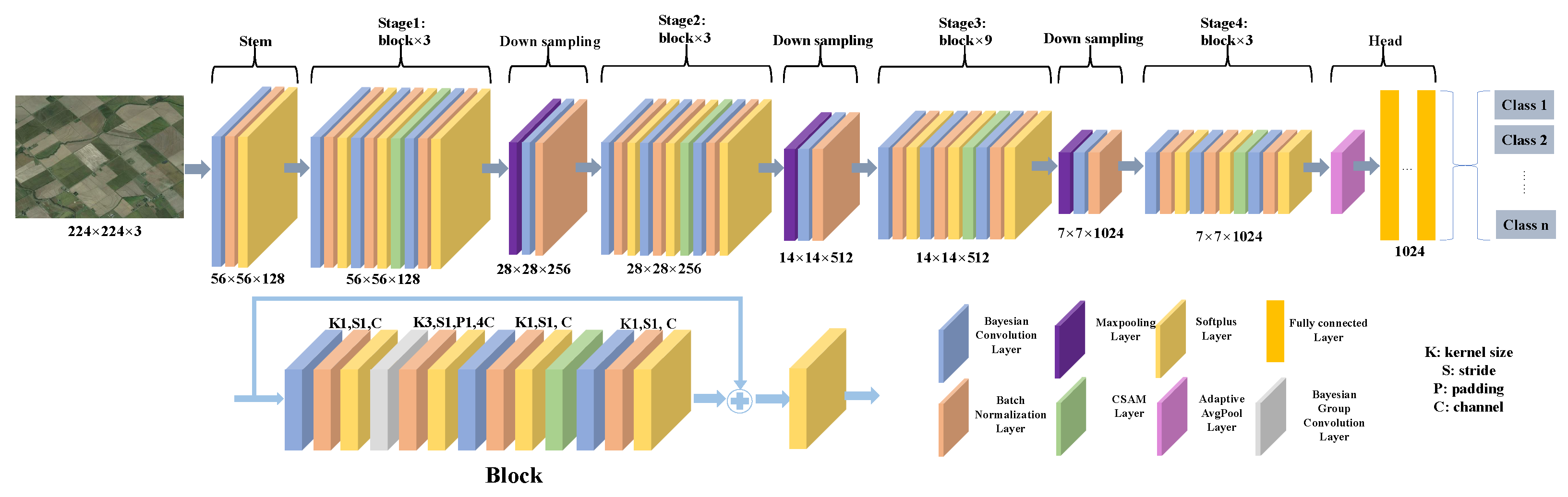
Remotesensing 16 00925 g001
Figure 2. The overall structure of the BayesNet model, which consists of stem, body, and head parts.
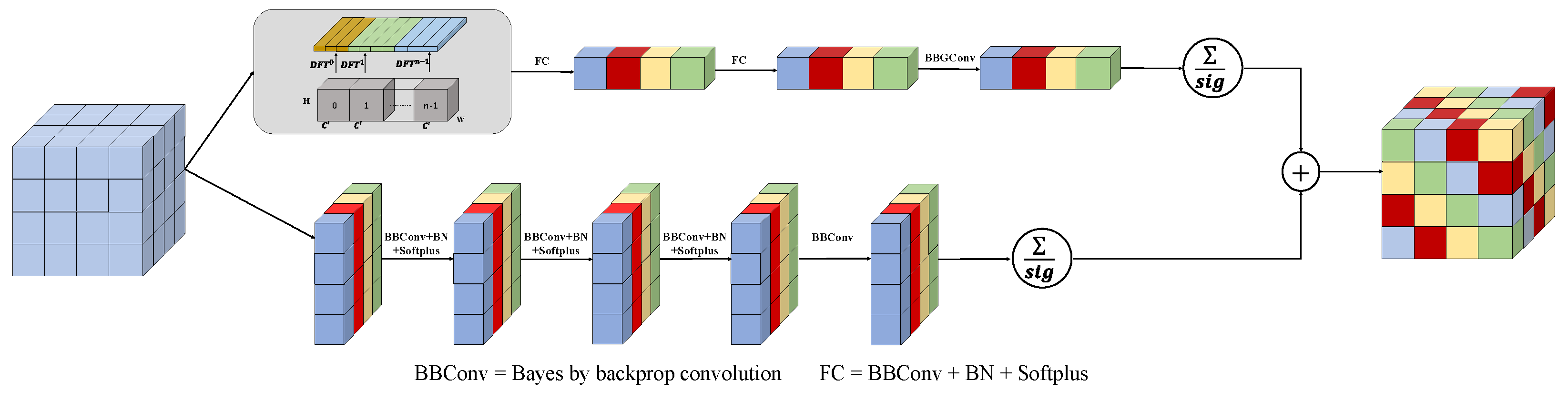
Remotesensing 16 00925 g002
Figure 3. The architecture of the CSAM block from the individual block, showcasing its detailed structure and components.
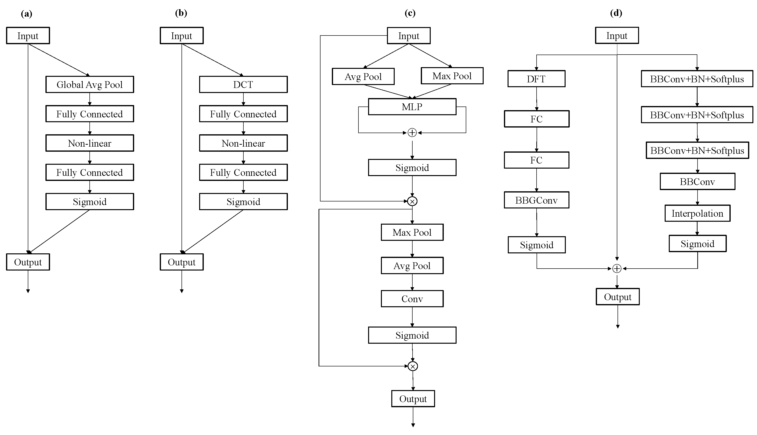
Remotesensing 16 00925 g003
Figure 4. The comparison of different structure of attention modules. (a) SE attention module, (b) FcaNet attention module, (c) CBAM attention network, (d) proposed CSAM attention module.
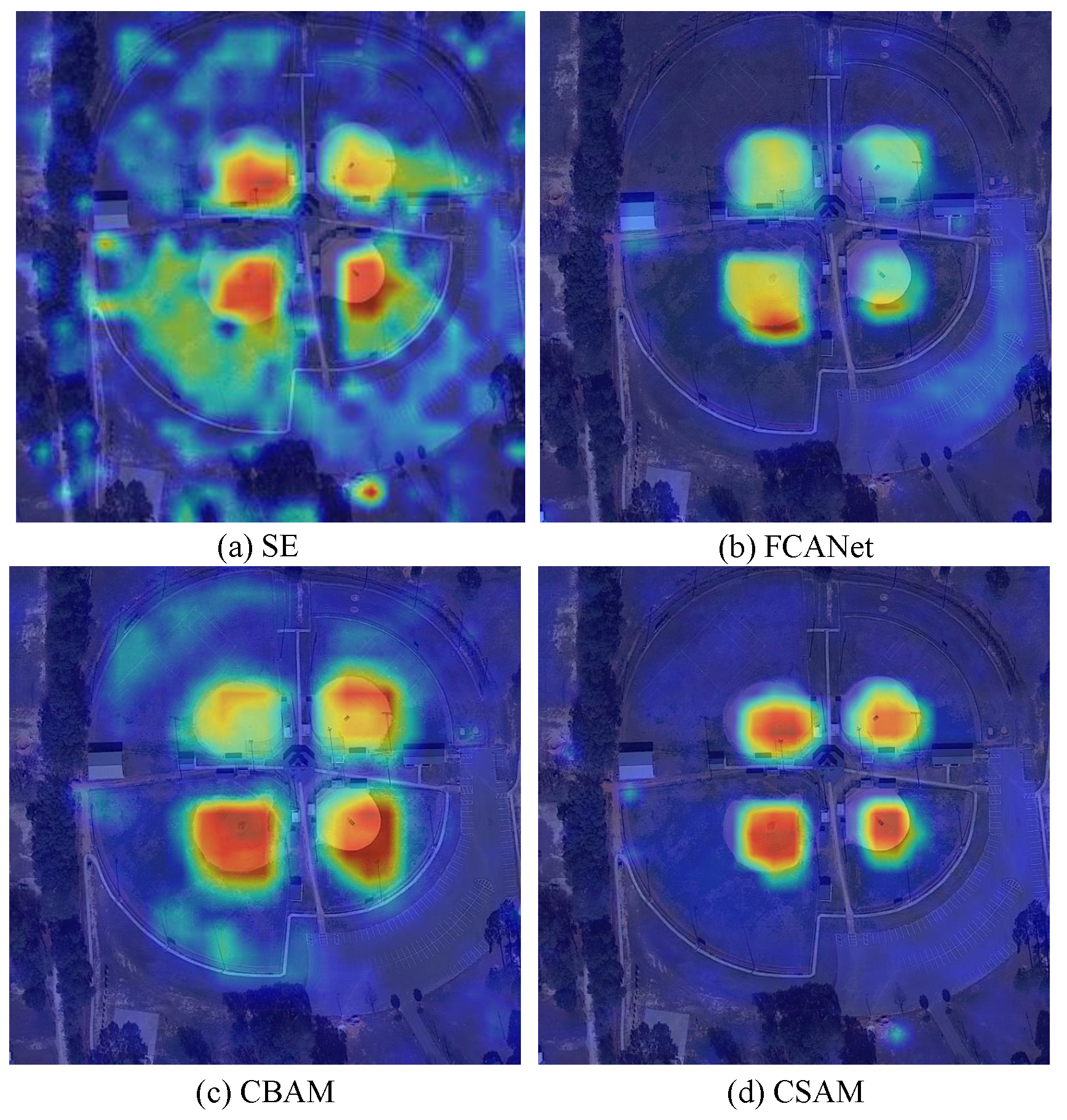
Remotesensing 16 00925 g004
Figure 5. The visual comparison of different methods using GradCam.
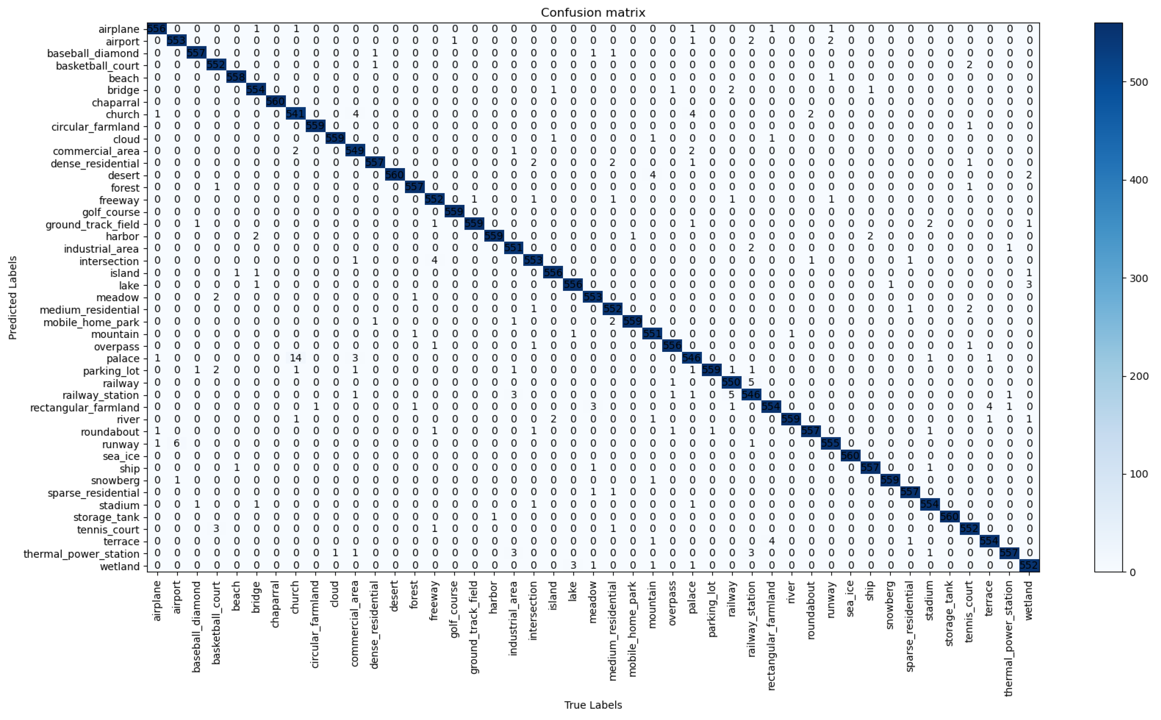
Remotesensing 16 00925 g005
Figure 6. The calculated confusion matrix on AID (50:50) dataset using BayesNet.
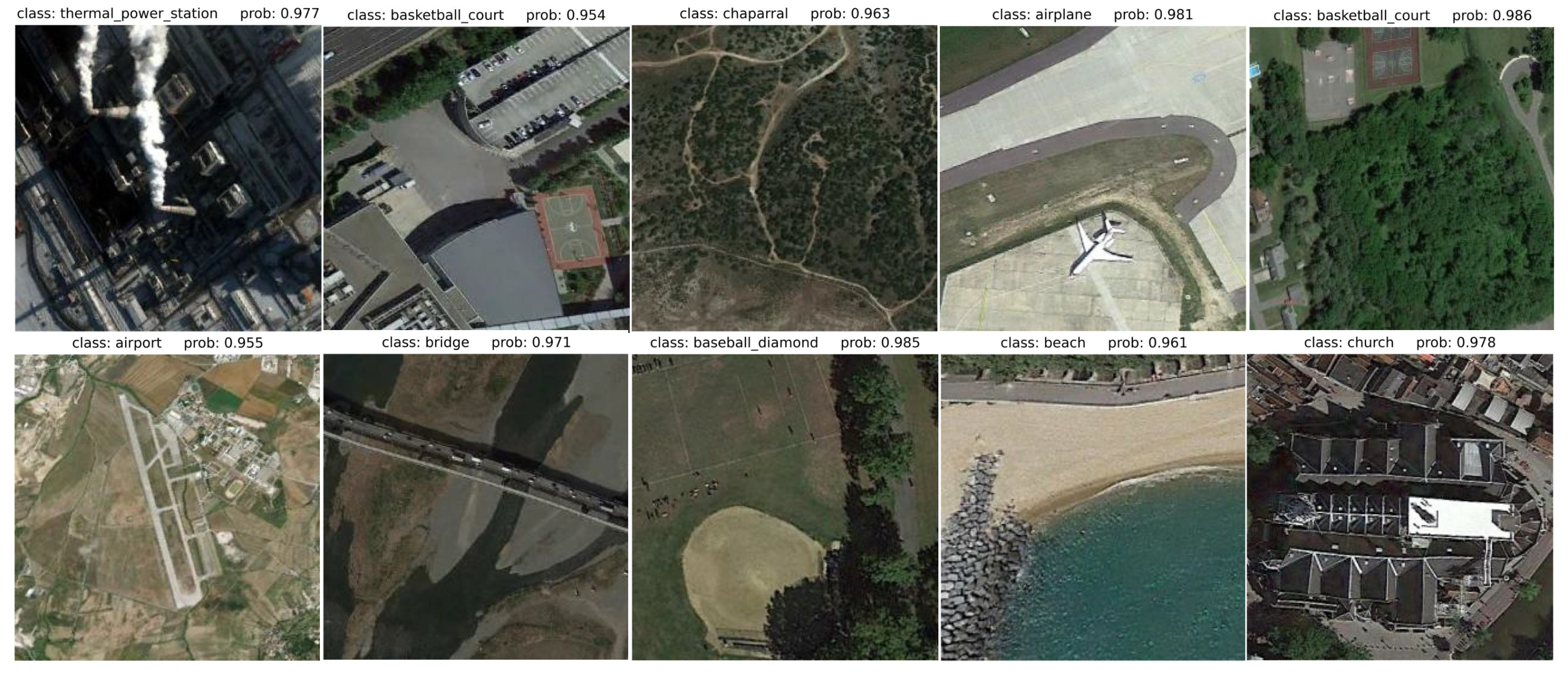
Remotesensing 16 00925 g006
Figure 7. Visualization of the efficient classification results of the BayesNet on the AID dataset.
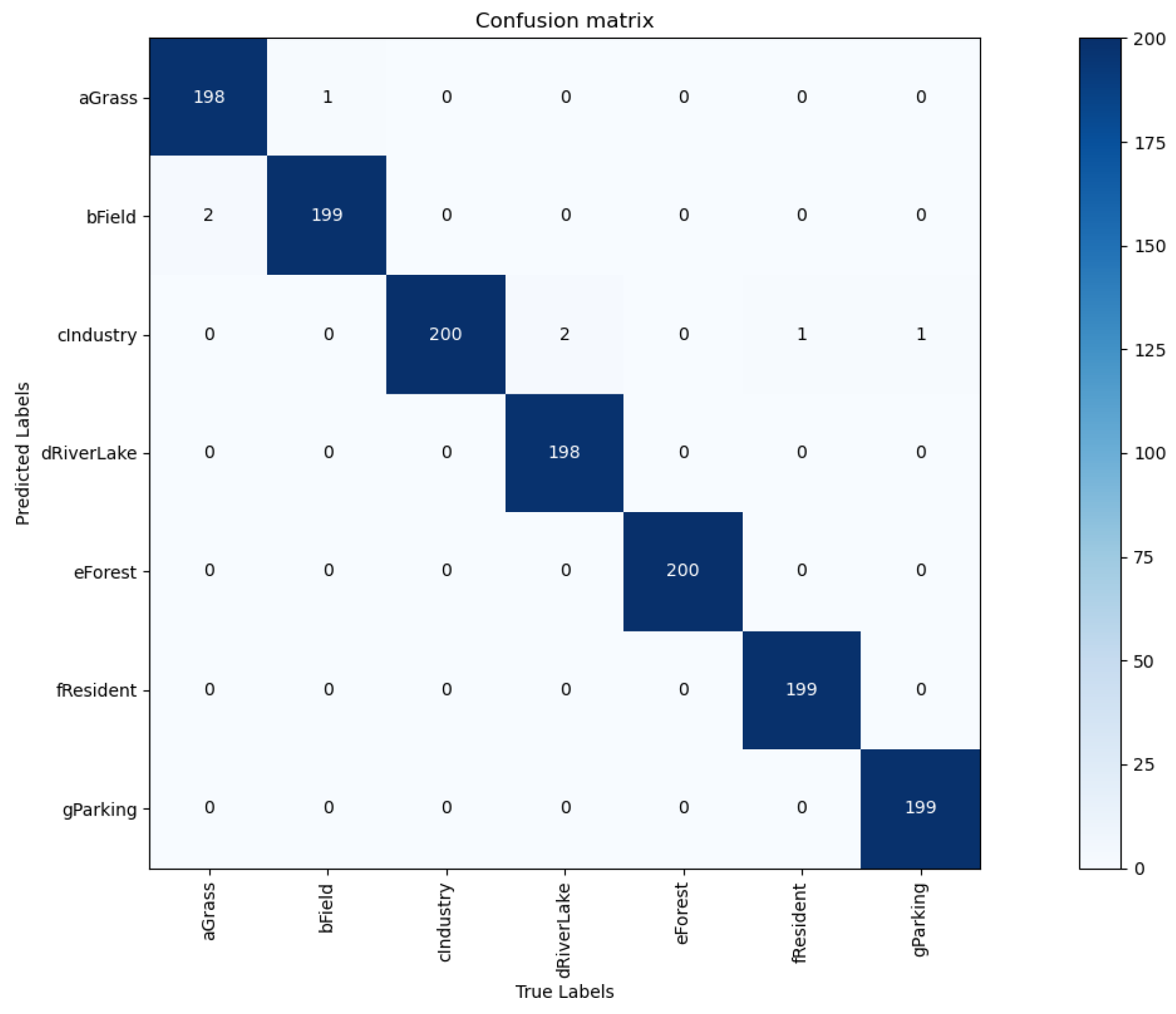
Remotesensing 16 00925 g007
Figure 8. The calculated confusion matrix on RSSCN7 (50:50) dataset using BayesNet.
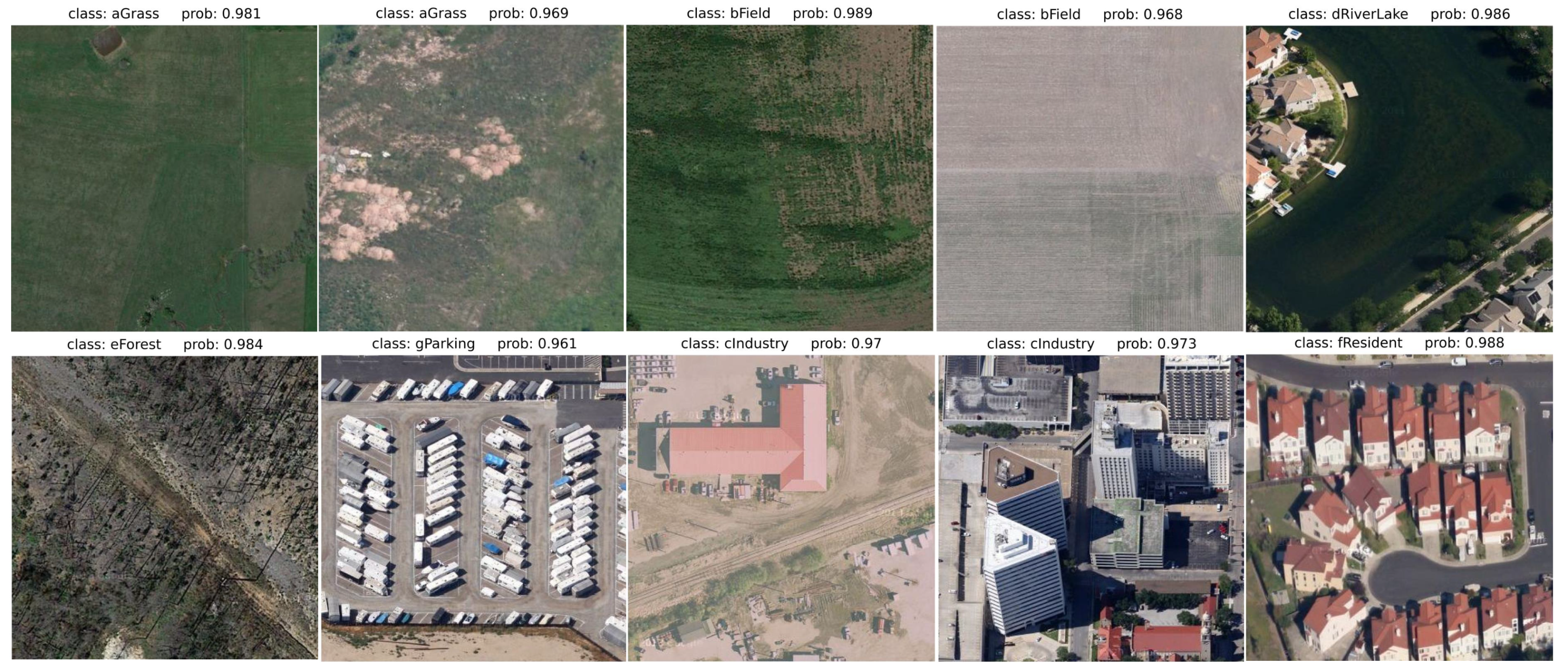
Remotesensing 16 00925 g008
Figure 9. Illustration of the robust classification performance of the BayesNet using the RSSCN7 dataset.
Remotesensing 16 00925 g009
Figure 10. The calculated confusion matrix on NWPU45 (20:80) dataset using BayesNet.
Remotesensing 16 00925 g010
Figure 11. Visualization of the efficient classification results of the BayesNet on the NWPU dataset.
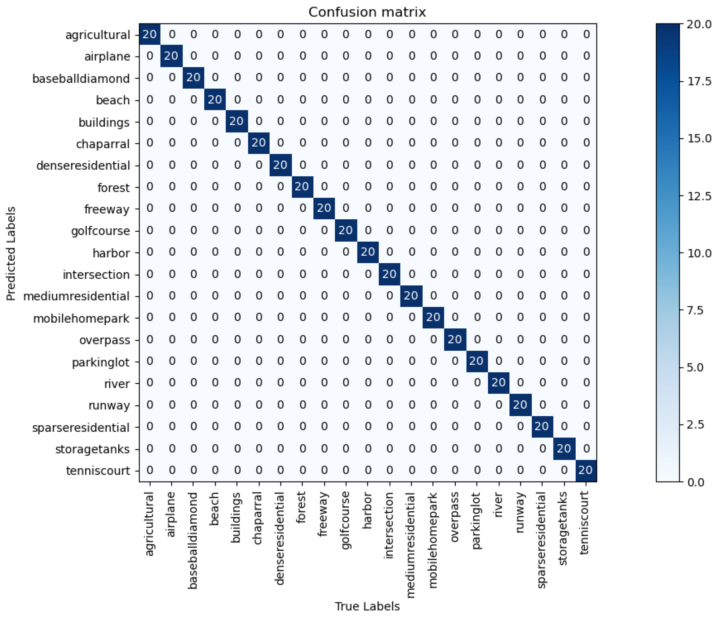
Remotesensing 16 00925 g011
Figure 12. The calculated confusion matrix on UCM21 (20:80) dataset using BayesNet.
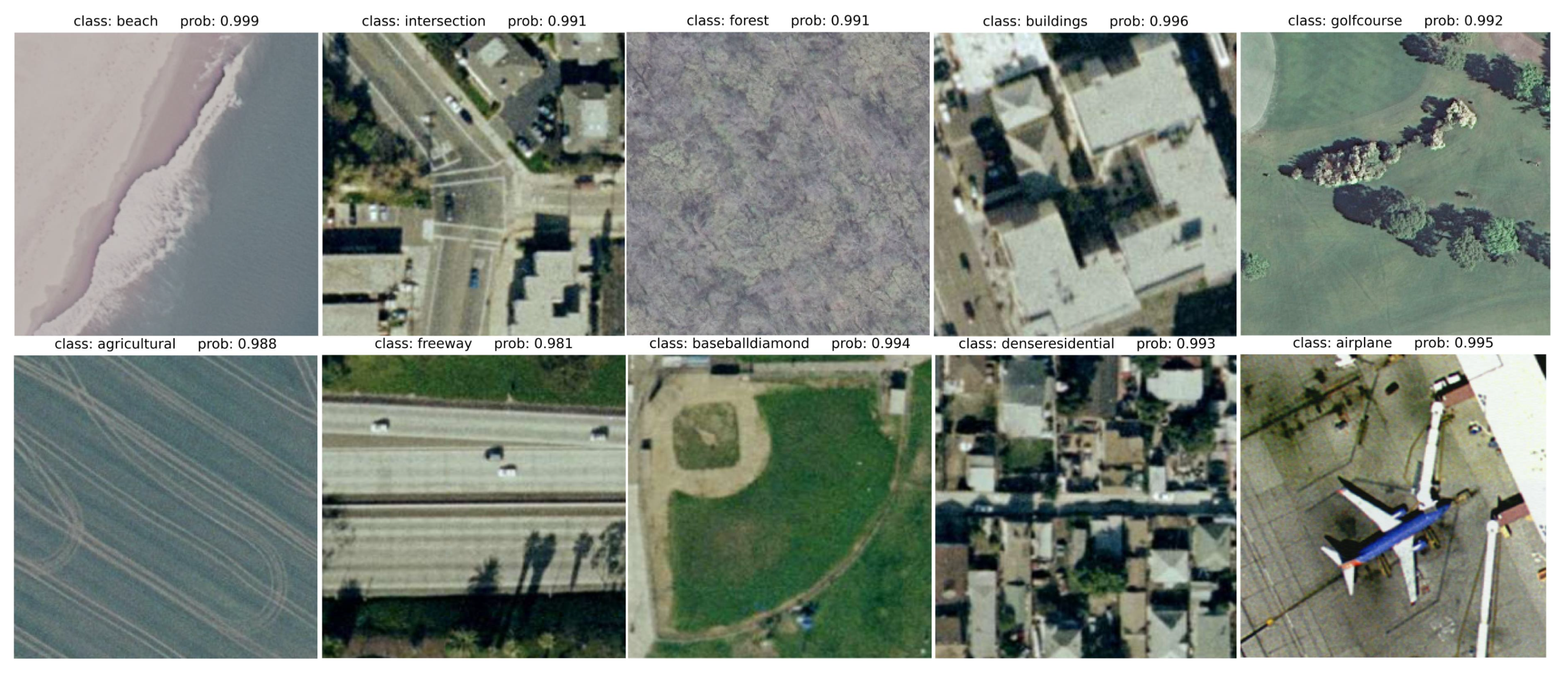
Remotesensing 16 00925 g012
Figure 13. Demonstration of the distinctive classification capabilities of the proposed BayesNet on UCM21 dataset.
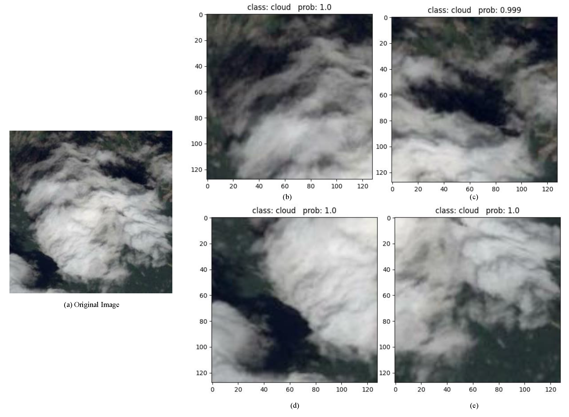
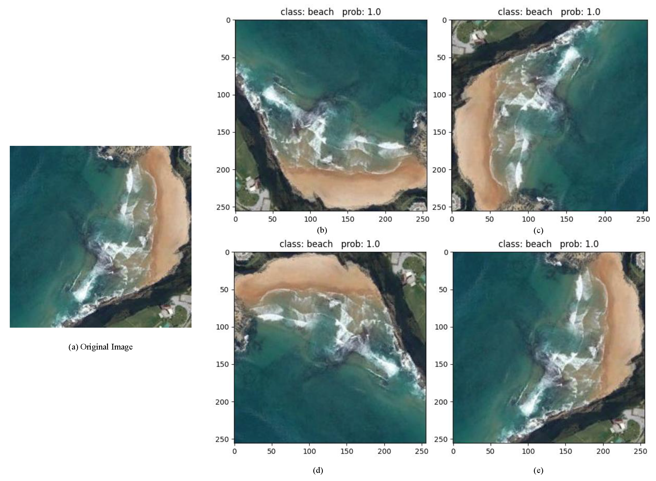
Remotesensing 16 00925 g013
Figure 14. The predictions of BayesNet on the cropped images. Cropped images were used to evaluate the performance of the BayesNet. (a) original image, (b) prediction on cropped top left of the original image, (c) prediction on cropped top right of the original image, (d) prediction on cropped bottom left of the image, (e) prediction on cropped bottom right of the original image.
Remotesensing 16 00925 g014
Figure 15. The predictions of BayesNet on the rotated images. Different rotated angle images were used to evaluate the performance of the BayesNet. (a) original image, (b) prediction on 90 degrees rotated image, (c) prediction on 180 degrees rotated image, (d) prediction on 270 degrees rotated image, (e) prediction on 360 degrees rotated images.
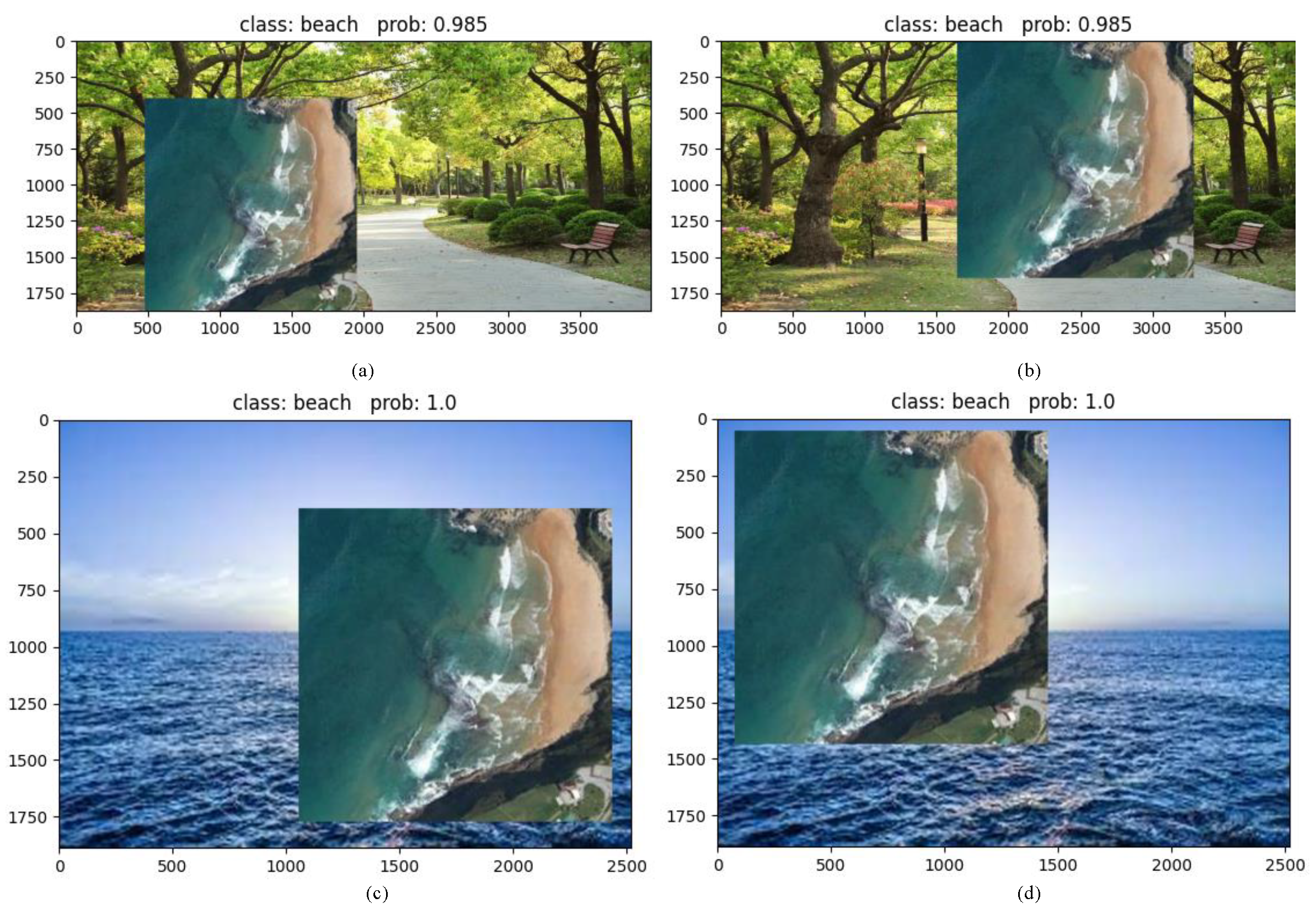
Remotesensing 16 00925 g015
Figure 16. The predictions of BayesNet on the partially overlapping images to evaluate the performance of the BayesNet in constrained environments. (a,b) prediction of beach class partially overlapped on park image; (c,d) prediction of beach class partially overlapped on sea image.
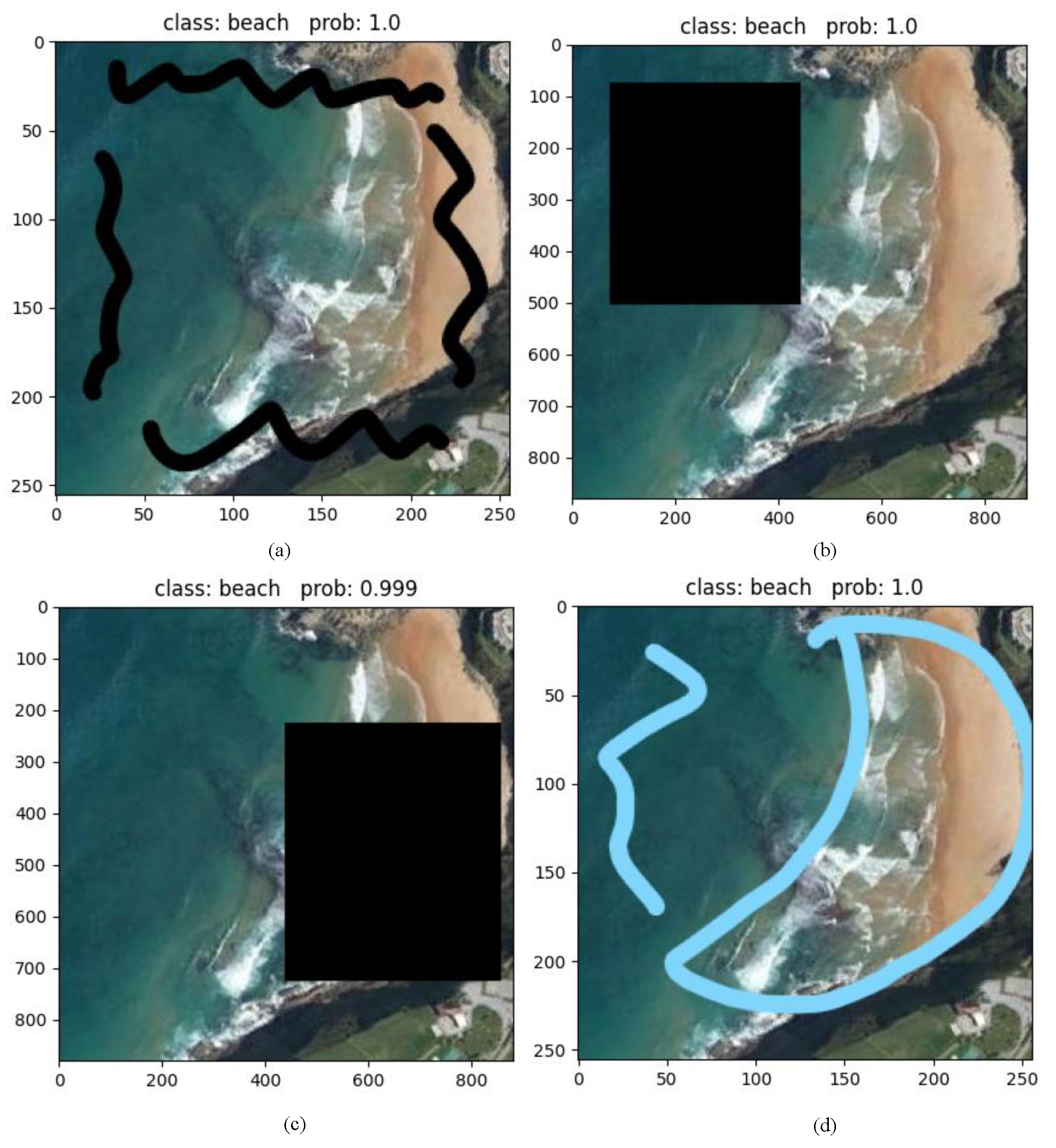
Remotesensing 16 00925 g016
Figure 17. The predictions of BayesNet on the noisy images, where black screen and random line noise were utilized to evaluate the performance of the BayesNet. (a) prediction of beach class with black line noise; (b) prediction of beach class with left aligned black screen noise; (c) prediction of beach class with right aligned black screen noise; (d) prediction of beach class with blue line noise.
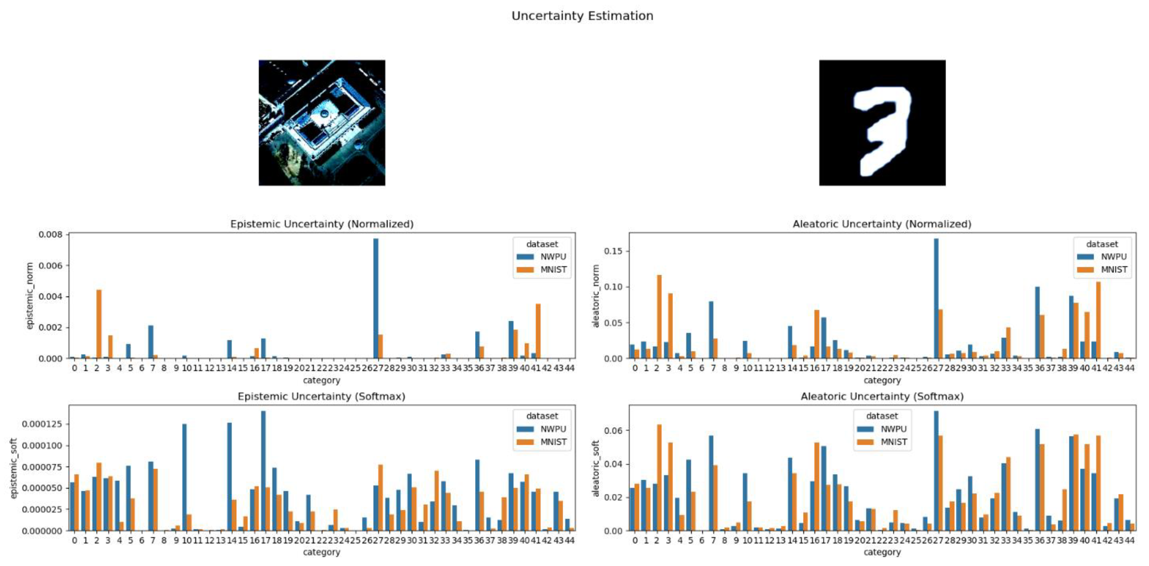
Remotesensing 16 00925 g017
Figure 18. The normalized and SoftMax aleatoric and epistemic uncertainty estimation for NWPU dataset using BayesNet.
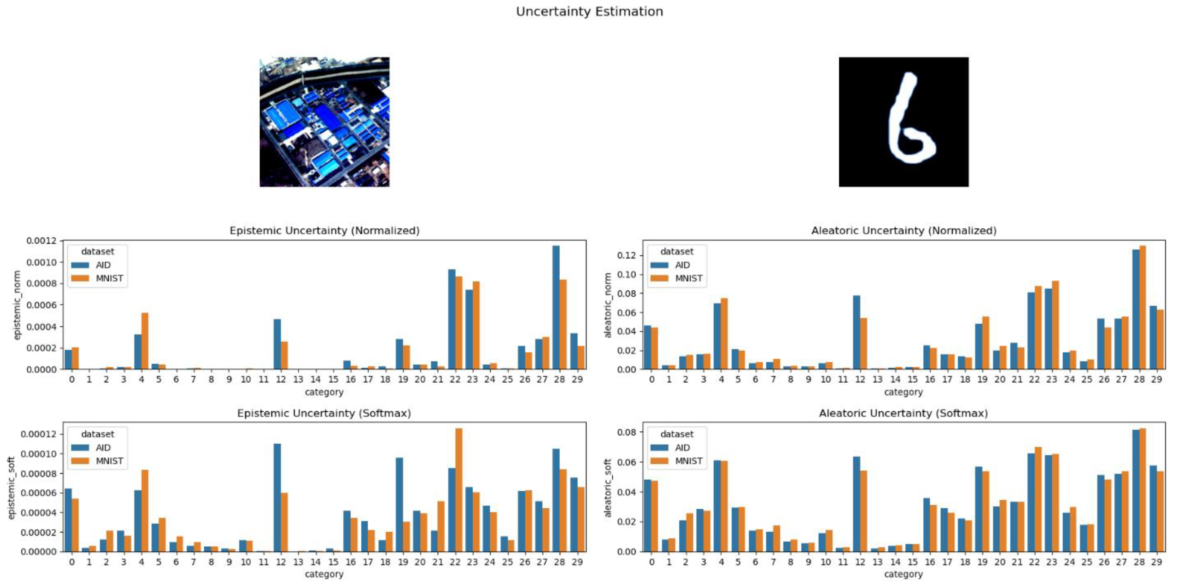
Remotesensing 16 00925 g018
Figure 19. Normalized and SoftMax-processed estimation of aleatoric and epistemic uncertainty for the AID dataset, utilizing BayesNet.
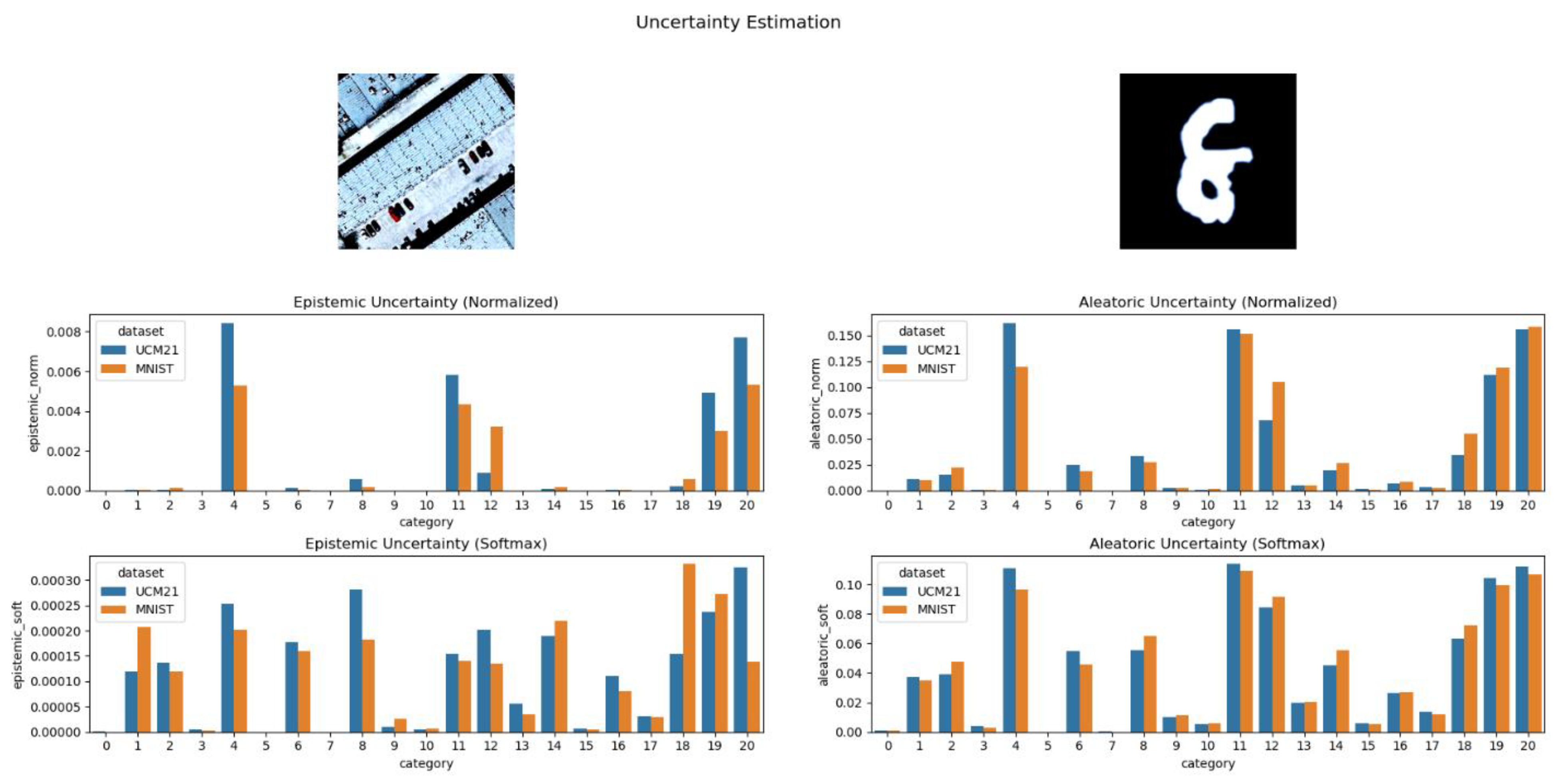
Remotesensing 16 00925 g019
Figure 20. Normalized and SoftMax-transformed representation of aleatoric and epistemic uncertainty estimation for the UCM-21 dataset, using BayesNet.
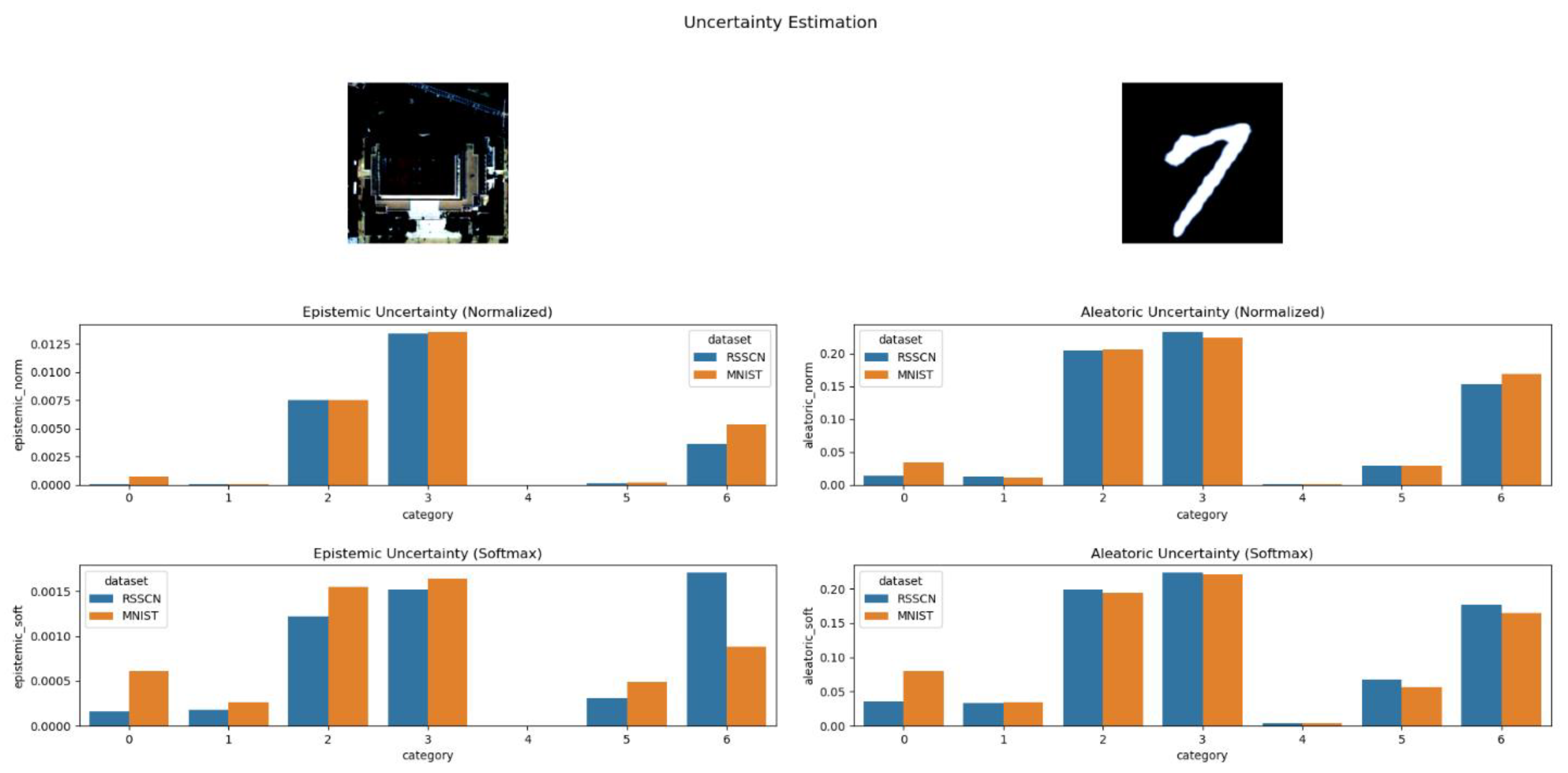
Remotesensing 16 00925 g020
Figure 21. Visualization of normalized and SoftMax-adjusted aleatoric and epistemic uncertainty estimations for the RSSCN7 dataset, leveraging BayesNet.
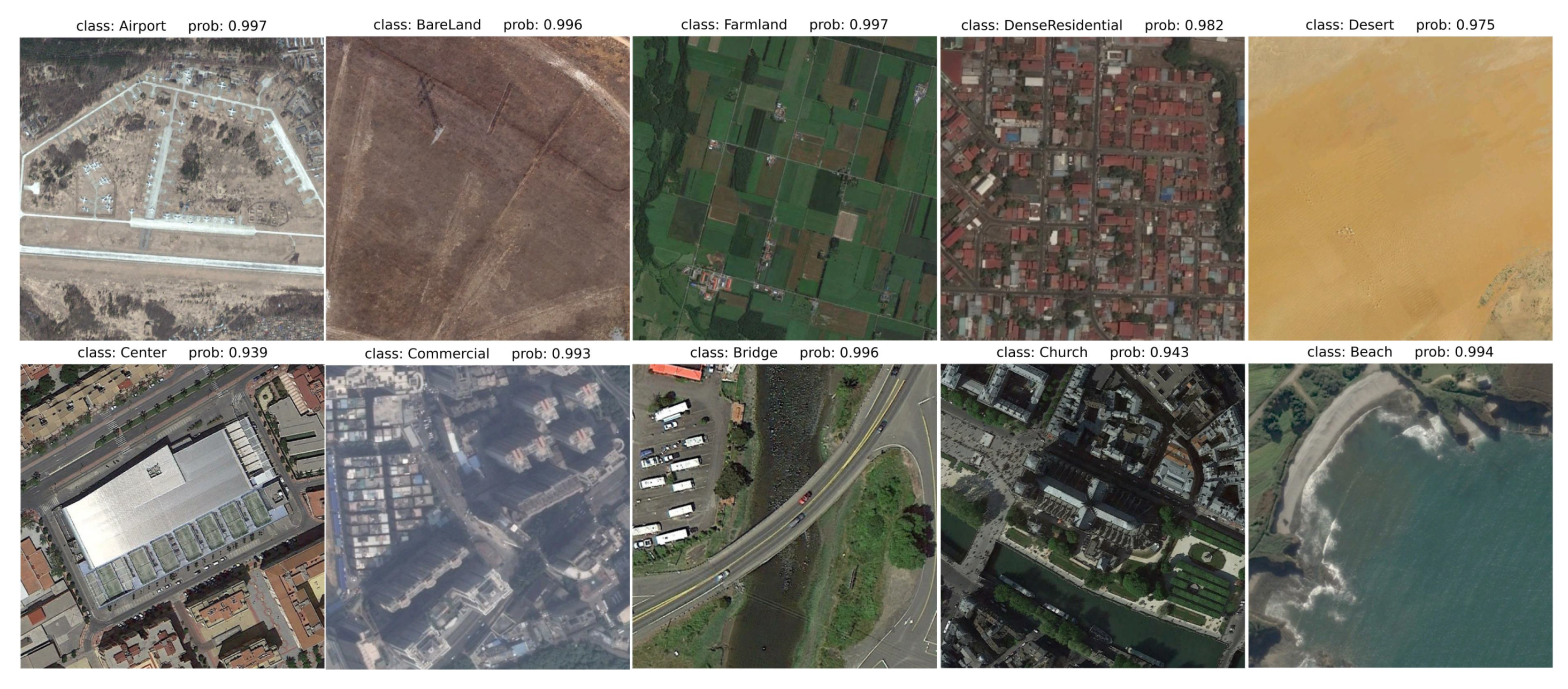
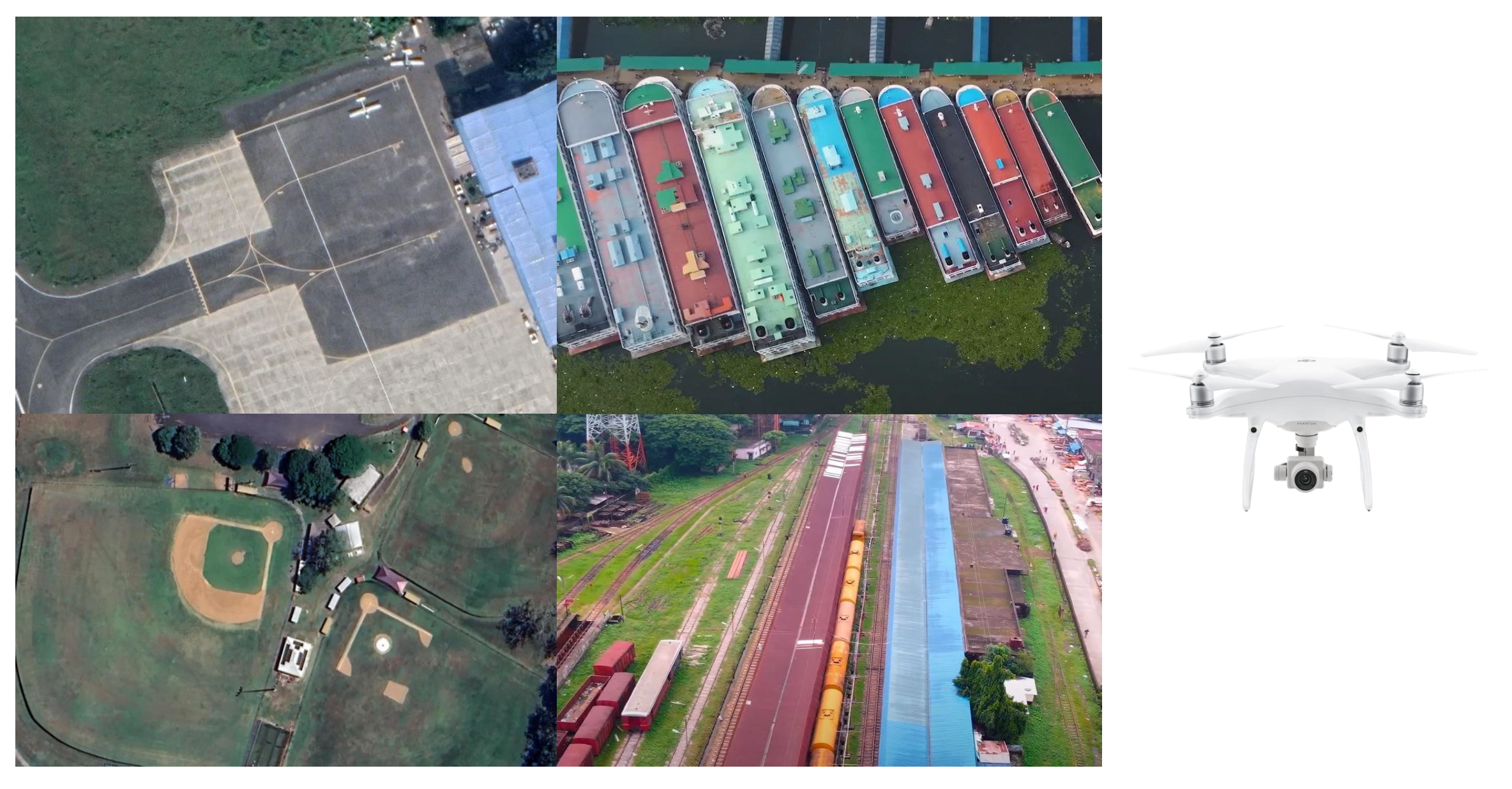
Remotesensing 16 00925 g021
Figure 22. Sample images from the testing dataset to evaluate the performance of BayesNet on unseen data.
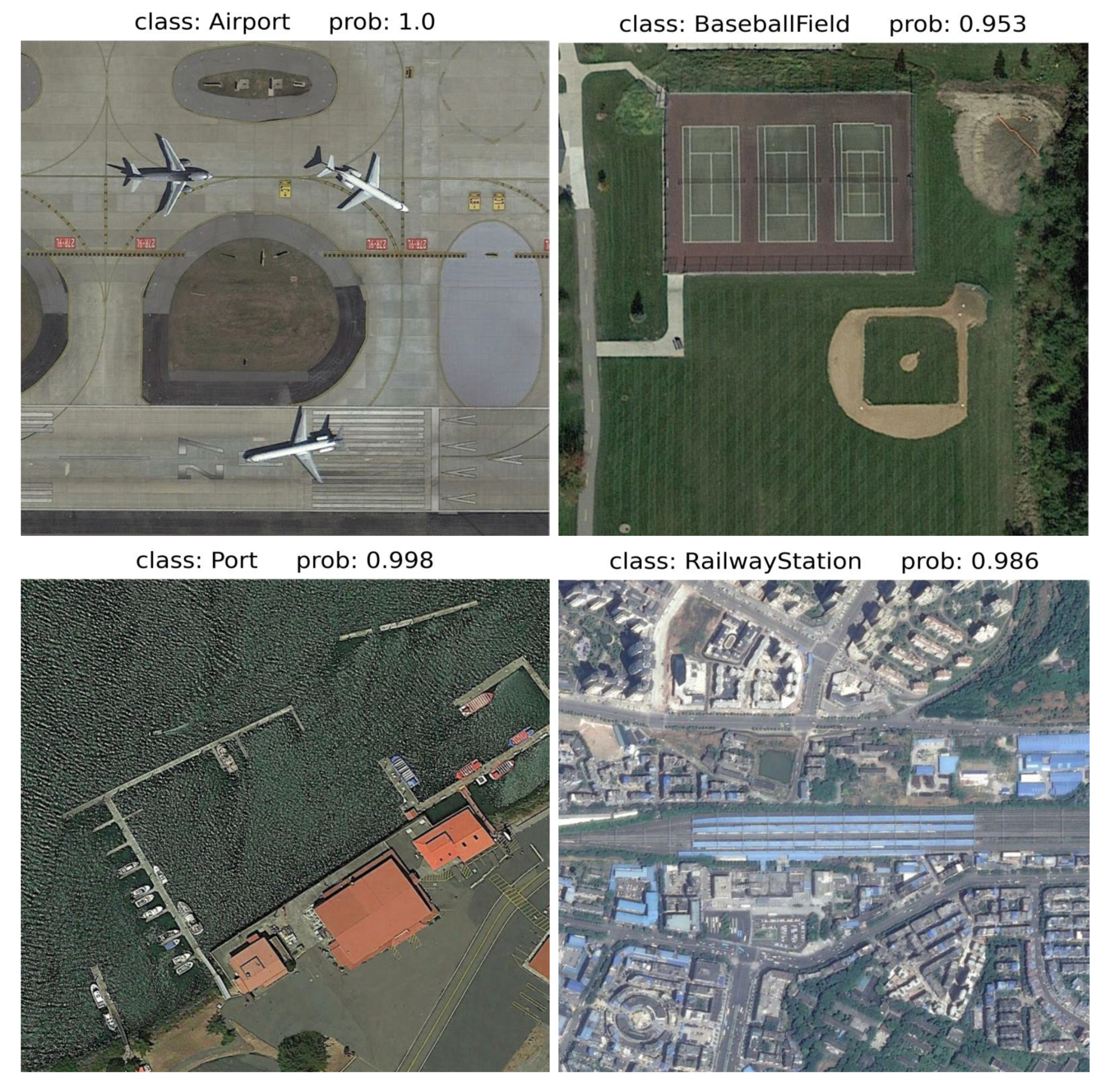
Remotesensing 16 00925 g022
Figure 23. Prediction visualization using BayesNet on our introduced remote sensing testing dataset which comprises complex backgrounds.
Remotesensing 16 00925 g023
Table 1. The detailed description of four remote sensing scene image datasets used in this study.
DatasetsScene Class NumberImage NumberImage ResolutionImage Size
UCM21 [23]2121000.3 256 × 256
RSSCN7 [24]72800--
AID [25]3010,0000.5–0.8 400 × 400
NWPU45 [26]4531,5000.2–30 600 × 600
Table 2. Comparative analysis of the accuracy (Acc) rates for different augmentation methods, including None, Auto-Augment, and the Proposed BayesNet (Flip, Clip, Perspective), across four datasets: UCM-21, RSSCN7, AID, and NWPU.
Augmentation MethodUCM21 [23]RSSCN7 [24]AID [25]NWPU [26]
None99.8797.2597.4695.32
Auto-Augment99.9397.3497.5195.39
BayesNet (Flip, Clip, Perspective)99.9997.3097.5795.44
Table 3. The training and testing accuracy of the BayesNet and the different deep learning models.
Model NameUCM21 [23]RSSCN7 [24]AID [25]NWPU [26]
AlexNet [30]88.1387.0085.7087.34
VGG16 [31]95.4487.1889.6493.56
GoogLeNet [32]93.1285.8486.3986.02
ResNet50 [33]94.7691.4594.6991.86
VIT [34]99.0190.8995.2793.31
RegNet [35]97.9394.3394.6195.03
Bayesian RegNet95.7295.2494.9395.05
BayesNet99.9997.3097.5795.44
Table 4. Comparative analysis of proposed models’ overall accuracy on AID dataset (50:50) over the last few years.
MethodYearOverall Accuracy
Bidirectional Adaptive Feature Fusion [36]201993.56
Feature Aggregation CNN [37]201995.45
Aggregated Deep Fisher Feature [38]201995.26
Skip-connected covariance network [39]201993.30
EfficientNet [40]202088.35
InceptionV3 [41]202095.07
Branch Feature Fusion [42]202094.53
Gated Bidirectional Network with global feature [43]202095.48
Deep Discriminative Representation Learning [44]202094.08
Hierarchical Attention and Bilinear Fusion [45]202096.75
VGG-VD16 with SAFF [46]202195.98
EfficientNetB3-CNN [47]202195.39
Multiscale attention network [48]202196.76
Channel Multi-Group Fusion [49]202197.54
Multiscale representation learning [50]202296.01
Global-local dual-branch structure [51]202297.01
Multilevel feature fusion networks [52]202295.06
Multi-Level Fusion Network [53]202297.38
MGSNet [54]202397.18
BayesNet-97.57
Table 5. Comparative analysis of proposed models’ overall accuracy on RSSCN7 dataset (50:50) over the last few years.
MethodYearOverall Accuracy
Aggregated Deep Fisher Feature [38]201995.21
SE-MDPMNet [55]201992.64
Positional Context Aggregation [56]201995.98
Feature Variable Significance Learning [57]201989.1
Branch Feature Fusion [42]202094.64
Coutourlet CNN [58]202195.54
Channel Multi-Group Fusion [49]202297.50
GLFFNet [59]202394.82
CRABR-Net [60]202395.43
BayesNet-97.30
Table 6. Comparative analysis of proposed models’ overall accuracy on NWPU45 (20:80) dataset over the last few years.
MethodYearOverall Accuracy
Rotation invariant feature learning [61]201991.03
Positional Context Aggregation [56]201992.61
Feature Variable Significance Learning [57]201989.13
Multi-Granualirty Canonical Appearance Pooling [62]202091.72
EfficientNet [40]202081.83
ResNet50 with transfer learning [41]202088.93
MobileNet with tranfer learning [41]202083.26
Branch Feature Fusion [42]202091.73
Multi-Structure Deep features fusion [63]202093.55
Coutourlet CNN [58]202189.57
Channel Multi-Group Fusion [49]202294.18
Multi-Level Fusion Network [53]202294.90
MGSNet [54]202394.57
BayesNet-95.44
Table 7. Comparative analysis of proposed models’ overall accuracy on UCM21 (80:20) dataset over the last few years.
MethodYearOverall Accuracy
Skip connected covariance network [39]201997.98
Feature aggregation CNN [37]201998.81
Aggregated Deep Fisher Feature [38]201998.81
Scale-Free Network [64]201999.05
SE-MDPMNet [55]201999.09
Multiple resolution BlockFeature method [65]201994.19
Branch Feature Fusion [42]202099.29
Gated Bidirectional Network with global feature [43]202098.57
Positional Context Aggregation [56]202099.21
Feature Variable Significance Learning [57]202098.56
Deep Discriminative Representation Learning [44]202099.05
ResNet50 with transfer learning [41]202098.76
VGG-VD16 with SAFF [46]202197.02
Coutourlet CNN [58]202199.25
EfficientNetB3 [47]202199.21
Channel Multi-Group Fusion [49]202299.52
Inception-ResNet-v2 [66]202399.05
MGSNet [54]202399.76
BayesNet-99.99
Table 8. The ablation study of the proposed model on four remote sensing datasets.
MethodUCM21 [23]RSSCN7 [24]AID [25]NWPU [26]
RegNet [35]97.9394.3394.6195.03
Bayesian + RegNet95.7295.2494.9395.05
RegNet + CSAM99.1496.7396.3195.18
BayeNet (Bayesian + Bayes Block + CSAM)99.9997.3097.5795.44
Table 9. The comparison of testing accuracy on our proposed dataset with AID dataset trained model.
MethodAccuracy
AlexNet [30]89.32
VGG16 [31]92.79
GoogLeNet [32]91.46
ResNet50 [33]94.57
ViT [34]95.35
RegNet [35]94.88
BayesNet96.39
Table 10. Comparison of parameters and complexity of different deep learning models implemented in this study.
MethodParameters (M)Complexity (G)
AlexNet [30]61.10.715
VGG16 [31]138.3615.5
GoogleNet [32]13.01.51
ResNet50 [33]25.564.12
VIT [34]306.5415.39
Bayesian RegNet900.392.3
BayesNet949.8593.1
Disclaimer/Publisher’s Note: The statements, opinions and data contained in all publications are solely those of the individual author(s) and contributor(s) and not of MDPI and/or the editor(s). MDPI and/or the editor(s) disclaim responsibility for any injury to people or property resulting from any ideas, methods, instructions or products referred to in the content.

