Article

Erosion Gully Networks Extraction Based on InSAR Refined Digital Elevation Model and Relative Elevation Algorithm—A Case Study in Huangfuchuan Basin, Northern Loess Plateau, China

1
College of Natural Resources and Environment, Northwest A&F University, Yangling, Xianyang 712100, China
2
College of Soil & Water Conservation Science and Engineering (Institute of Soil and Water Conservation), Northwest A&F University, Yangling, Xianyang 712100, China
*
Author to whom correspondence should be addressed.
Remote Sens. 2024, 16(5), 921; https://doi.org/10.3390/rs16050921
Submission received: 8 January 2024 / Revised: 9 February 2024 / Accepted: 23 February 2024 / Published: 6 March 2024
(This article belongs to the Special Issue Soil Erosion Estimation Based on Remote Sensing Data)

Abstract

:
The time-effective mapping of erosion gullies is crucial for monitoring and early detection of developing erosional progression. However, current methods face challenges in obtaining large-scale erosion gully networks rapidly due to limitations in data availability and computational complexity. This study developed a rapid method for extracting erosion gully networks by integrating interferometric synthetic aperture radar (InSAR) and the relative elevation algorithm (REA) within the Huangfuchuan Basin, a case basin in the northern Loess Plateau, China. Validation in the study area demonstrated that the proposed method achieved an F1 score of 81.94%, representing a 9.77% improvement over that of the reference ASTER GDEM. The method successfully detected small reliefs of erosion gullies using the InSAR-refined DEM. The accuracy of extraction varied depending on the characteristics of the gullies in different locations. The F1 score showed a positive correlation with gully depth (R2 = 0.62), while the fragmented gully heads presented a higher potential of being missed due to the resolution effect. The extraction results provided insights into the erosion gully networks in the case study area. A total of approximately 28,000 gullies were identified, exhibiting pinnate and trellis patterns. Most of the gullies had notable intersecting angles exceeding 60°. The basin’s average depth was 64 m, with the deepest gully being 140 m deep. Surface fragmentation indicated moderate erosive activity, with the southeastern loess region showing more severe erosion than the Pisha sandstone-dominated central and northwestern regions. The method described in this study offers a rapid approach to map gullies, streamlining the workflow of erosion gully extraction and enabling efficiently targeted interventions for erosion control efforts. Its practical applicability and potential to leverage open-source data make it accessible for broader application in similar regions facing erosion challenges.

1. Introduction

Gully erosion is a widespread land degradation form that is occurring around the globe [1]. It is a large source of sediment yield, usually accounting for 20~90% depending on the landscape [2,3]. Consequently, the nutrient content, like the soil organic carbon, in the topsoil decreases due to the transportation of soil and sediment [4]. The development of erosion gullies also shrinks the area of usable land by fragmenting the morphology of a surface that was once flat, forming a rugged terrain consisting of numerous gullies that link into networks [5,6]. Gully erosion has become a key concern in many regions around the world over the past century [7]. Therefore, monitoring the development of erosion gullies via extracting and mapping has become vital for enacting prevention strategies.
Efforts to monitor erosion gully have evolved over time. Traditional methods include field surveys and manual extraction of erosion gullies from satellite images, which are labor-intensive and time-consuming methods [6]. Zhao et al. [8] developed a random point sampling method for the rapid estimation of the presence of erosion gullies. However, detailed information on gully characteristics such as morphology, depth, and width is crucial for water and soil conservation studies. Therefore, the extraction of entire gullies within specific regions is still necessary. Technological advancements, such as LiDAR and unmanned aerial vehicles (UAVs), have provided high-resolution data, enabling object-based gully extraction [9,10]. Existing efforts that have been dedicated to erosion gullies extraction can be classified into two categories.
Category I is mainly supported by computer vision and deep learning. UAVs and open archives of high-resolution optical satellites (e.g., Google Earth Imagery, Esri World Imagery, etc.) provide orthographic observation of erosion gullies. By applying deep learning models with different architectures (e.g., SegNet, U-net, R2-Unet, etc.), computers obtain the features of a gully and classify the gully pixels on images to accomplish erosion gully extraction tasks [11,12]. Although these methods can generate fine boundaries, the labeling and training process is time-consuming and sensitive to the image color uniformity, contrast, and quality. For tasks covering large areas, small UAVs are unsuitable due to economic decline, and the use of high-resolution satellite images greatly increases the cost. Additionally, three-dimensional attributes such as the depth of a gully cannot be obtained from images. Xue et al. suggested a method to obtain three-dimensional river networks with a relatively novel effect. However, this workflow is mainly designed for larger river systems and may not be able to obtain information from small erosion gully networks [13].
Category II takes advantage of the digital elevation models (DEMs), a rasterized digital expression of the Earth’s surface terrain, to detect abrupt topographic points as the identifier of gullies. These methods are elaborately designed mathematically, such as the window sliding algorithm developed on finite morphologic element theory [14], the active contours method using the snake model [15], edge detection based on the LOG operator [16], and the Marr–Hildreth operator [17]. However, there is a tradeoff between accuracy and computation cost when applied to a large area. Moreover, the rapid development of erosion gullies in highly eroded areas may outdate the available public DEM datasets, hindering the quasi-real-time extraction and monitoring of erosion gullies at the regional scale.
Notably, the mentioned methods in these two categories are currently limited to smaller areas due to time and cost constraints. There is a pressing need to develop extraction methodologies that consider gully networks as an interconnected system [18]. Such approaches would enable a more comprehensive understanding of the advancing progress of gully erosion. Additionally, existing methods encounter challenges in identifying gully type (e.g., gully bank, gully floor, etc.) because a physically meaningful classification scheme and a corresponding feasible method are still lacking [6]. Currently, the definition of gullies that can distinguish their boundary from fragmented landscapes remains ambiguous, hindering the intactness of gullies’ extraction from available data. While the lower bound of the critical cross-sectional area of a gully is usually defined as the size that conventional tillage practices cannot erase [19], the upper bound remains unclear in the existing literature [6]. In the Chinese Loess Plateau, the shoulder line is commonly treated as the boundary of erosion gullies [20], as the slope below this line increases dramatically (usually > 35°).
Interferometric synthetic aperture radar (InSAR) can detect deformations of the Earth’s surface by comparing the phase difference of two different SAR images with slightly different antenna positions [21]. With its all-day functioning, short-interval revisiting, cloud-penetrating ability, and high-resolution detection, SAR provides considerable potential for time sequence DEM reconstructing [22] and in long-term gully erosion studies. Moreover, leveraging the phase information offered by InSAR enables the measurement of slight topographic variations and the generation of DEM with enhanced relief details [23]. These additional details facilitate more accurate erosion gully extraction. Additionally, SAR satellites provide cost-effective data covering a wide range of areas [24,25], allowing for the rapid acquisition of DEMs and improvement in DEM quality, particularly in capturing surface gully features. This approach partially overcomes the limitations of traditional DEM extraction methods. The existing literature has proven that InSAR-based methods are efficient in detecting surface deformation and thus reconstructing DEM with relatively high accuracy. Berardino et al. [26] proposed a small orbital separation baseline (SBAS) to limit spatial decorrelation and detect ground deformation in southern Italy on a small map scale. Zhao et al. [27] examined a large-map-scale loess landslide in Shaanxi, China, using improved SBAS by checking DEM errors with a coherence threshold and determining interferogram quality in advance to suppress imprecise elevation correction. The launch of Sentinel-1 (S1) made the open access of spaceborne radar imagery possible. Even though this project was not primarily designed for DEM reconstruction, the available imagery still meets the basic requirements for DEM reconstruction with a careful selection of image pairs [23].
The relative elevation algorithm (REA) removes the downward trend in floor elevation by respecting the baselines along the bottom of gullies [28]. It is generally known that gully floors always have a downward trend (the decreasing trend of floor elevation) extending from upper gully heads to lower confluences or outlets because of the close relationship between gully erosion and hydrologic processes. This limits small-map-scale gully extraction, as the descending elevation along the longitudinal gully-flow profile cannot be ignored, and the contours of the gully bank are always convergent. By applying REA, a floor-equal elevation model enhancing the cross-sectional characteristics of gullies can be derived. This algorithm is often applied to fluvial geomorphology as a cartographic expression for visual enhancement, but it also shows great potential in gully extraction. With the removal of the downward trend, the elevations at different terrain locations are numerically clustered, facilitating the classification of gully types and overcoming the limitation of the traditional methods that only extract gully boundaries without acquiring three-dimensional information from the inner gully area.
The Loess Plateau (LP) in north-central China is characterized by extensive gully formation, primarily due to the erodible loess soil and prolonged inappropriate land management practices [29]. The Huangfuchuan Basin, recognized as one of the most eroded areas within the Loess Plateau, is significant as it is designated as one of China’s eight national key management areas [30]. These erosional activities have significantly increased sediment transport in the Yellow River, contributing to the increased silting of river beds and heightened risks of ecological destruction [31,32]. Consequently, the development of extensive gully networks in this basin has established it as a prime location for studying erosion gully extraction, given its typical gully landforms and practical significance (Figure 1). In this study, we developed a workflow that integrates InSAR-reconstructed DEMs with REA for the rapid extraction of gully networks in a selected typical gully erosion watershed in the LP. The objectives of this study were to reconstruct digital elevation models (DEMs) and extract gully networks in the study area, and to analyze the spatial characteristics of the gully networks, as well as the performance of the method.

2. Materials and Data
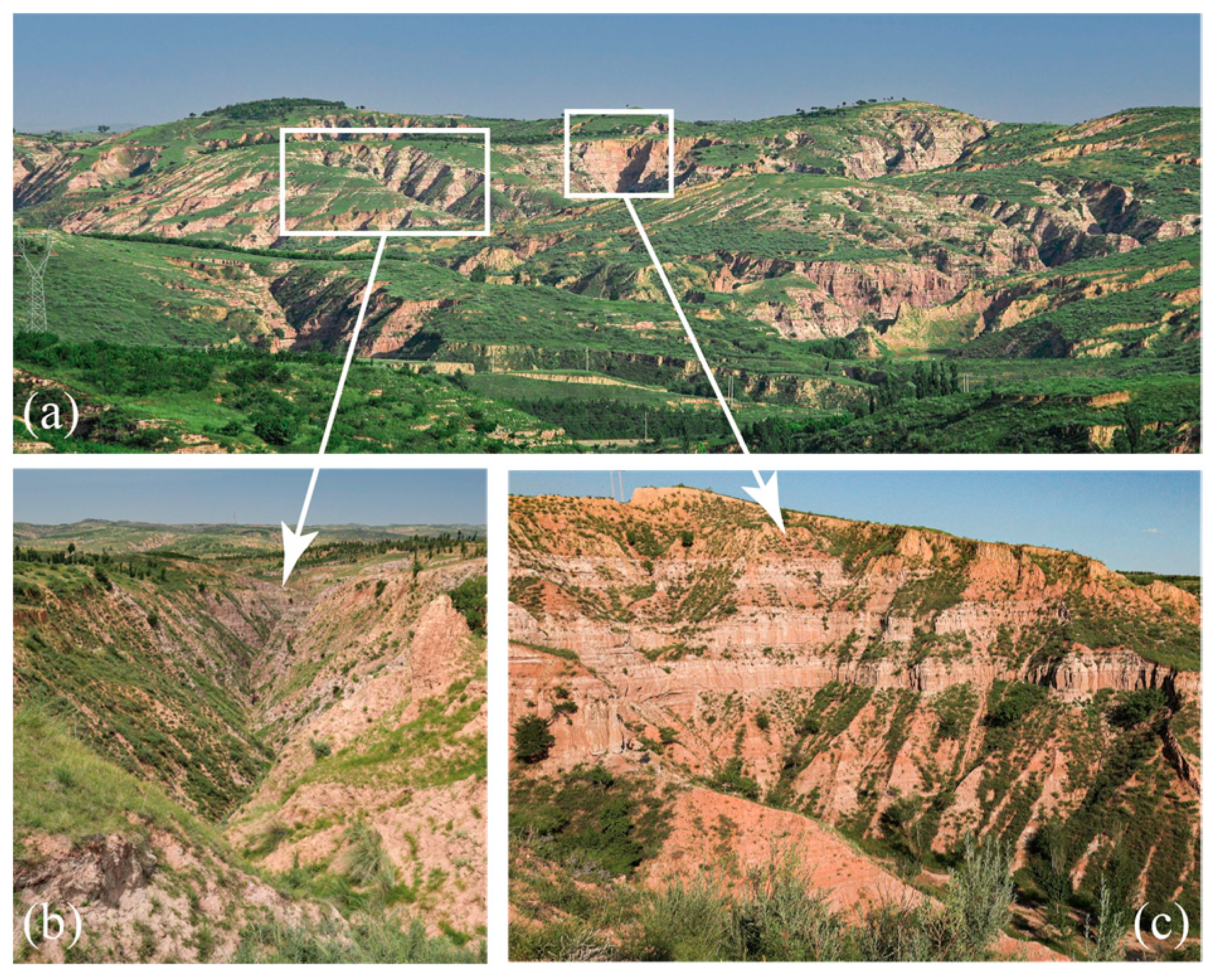
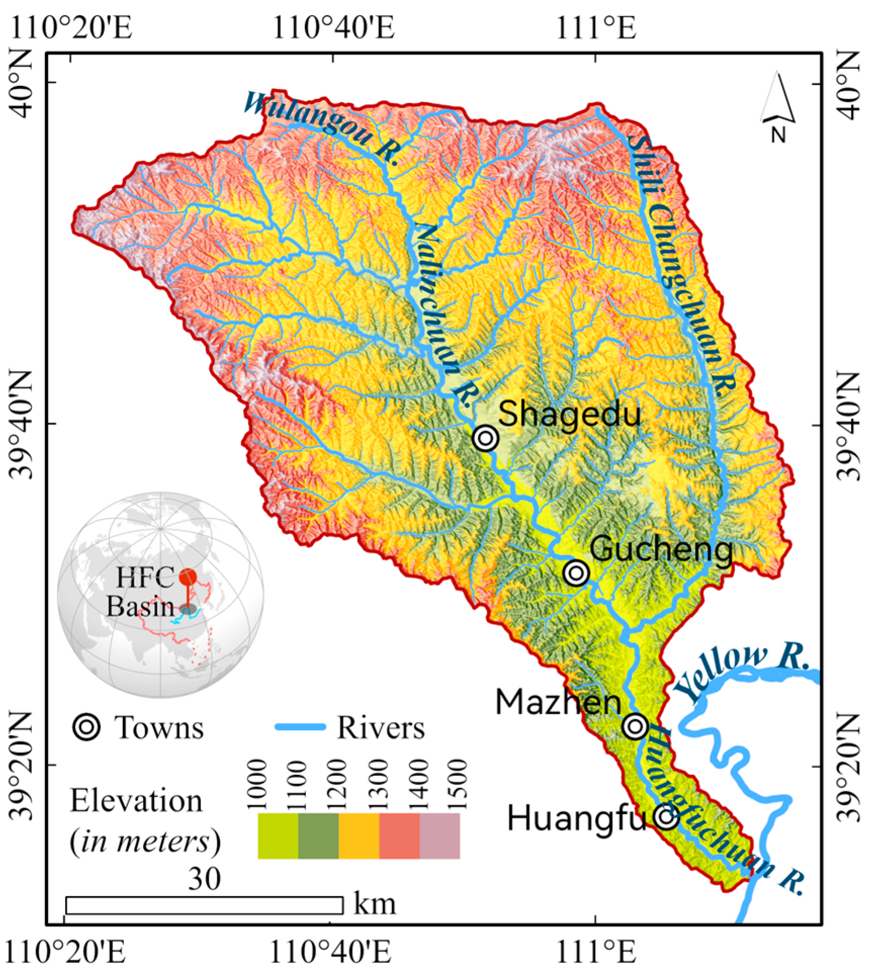
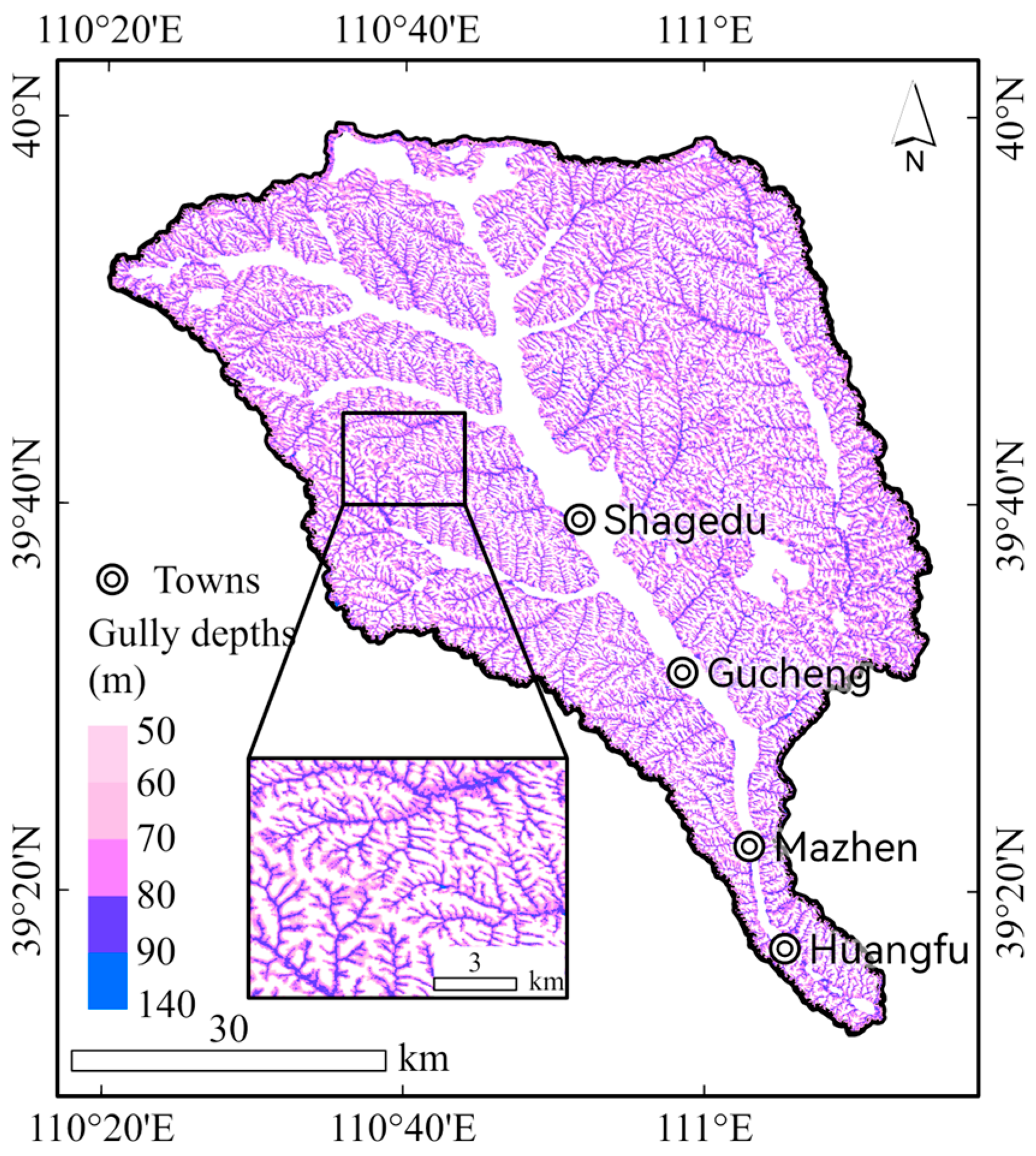
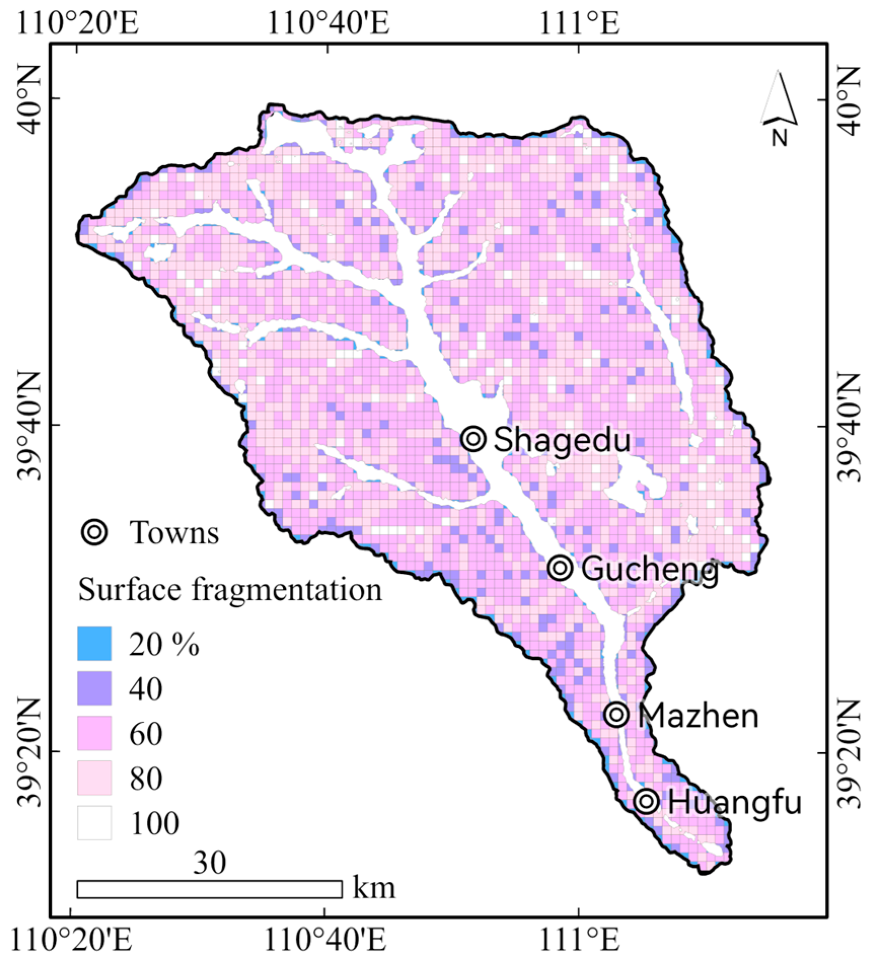
2.1. Study Area

The Huangfuchuan River (HFC) basin (Figure 2) was selected as the study area to represent a typical loess gully basin suffering from intensive gully erosion. The HFC originates in northern Jungar Banner, Inner Mongolia Autonomous Region, and flows 125.1 km into the Yellow River in Fugu County, Shaanxi Province. The HFC drainage basin (39°12.7′~39°59.6′N, 110°20.3′~111°15.0′E) covers 3240 km2 in the northern semiarid Loess Plateau region, with elevations ranging from 820 to 1440 m. This region has been experiencing uplift since the Quaternary period, resulting in diverse forms of erosion gullies [33]. Gully depths average 40–70 m, with some exceeding 100 m. The composition of the soil within the HFC basin predominantly consists of Pisha sandstone and loess. Pisha sandstone is a local soil texture that mainly covers the northern Loess Plateau. The feldspar in the Pisha sandstone, primarily weathered by kaolinite, exhibits low erosion resistance and serves as the primary mineral contributing to the sandstone’s susceptibility to erosion [34,35]. Loess features a unique structure where clay-size particles coat silt grains and gather at quartz contacts, resulting in high porosity and macroscopic pores. Its soil properties are influenced by microstructure, making it prone to collapse and sliding when wet [36,37]. Both these soil types exhibit weak bonding and low compressive strength, which contribute to the basin’s susceptibility to significant soil erosion [38]. The annual erosion modulus has been estimated as between 3000 and 4000 tons per square kilometer [39]. The northern region of the basin is characterized by a prevalence of Pisha sandstone, while the southern region is dominated by collapsible loess. Vegetation cover, primarily Caragana korshinskii, coniferous Prunus armeniaca (apricot), and Pinus massoniana (masson pine), decreases from southeast to northwest. Crop fields are distributed near the main HFC channel and intergully tableland area, having a gentle slope. The predominant crop types are Zea mays (maize) and Panicum miliaceum (millet). The average annual temperature is 9.1 °C, and precipitation is 350~450 mm, with extreme rainfall in July (mean 92 mm) occurring due to the continental monsoon. This results in an average of 61.2 million tons of sediment yield annually, with heightened summer fluvial erosion. Extensive water and soil conservation projects, chiefly check dams (sediment-trapping dams) and terraced fields, have been implemented across the basin. These distinct characteristics of the HFC make it an ideal area for researching hydraulic erosion gullies in the Loess Plateau.

2.2. Data

2.2.1. SAR Data

Sentinel-1 interferometric wide (IW) swath data distributed in Level-1 single look complex (L1 SLC) products were used in this study. Original SAR data were acquired by the Terrain Observation with Progressive Scans SAR (TOPSAR) on the Sentinel-1. The spatial resolution was 5 m × 20 m in a single look. Data from the L1 SLC products were 2.3 m × 14.1 m gridded for universal agreement in range and azimuth while preserving phase information. As suggested by Alessandro et al. [40], suitable temporal and perpendicular baseline (150–300 m) are two vital requirements that need to be met when selecting suitable image pairs, because improper selection may lead to failure in DEM reconstruction due to the signal being out of phase. Moreover, low water vapor in the atmosphere and low vegetation coverage on land are also suggested to avoid phase delay and temporal decorrelation. Following these principles, we selected and downloaded available data (Table 1) from the Data Search Vertex of Alaska Satellite Facility (https://search.asf.alaska.edu, accessed on 10 December 2023) [41].

2.2.2. Auxiliary Data
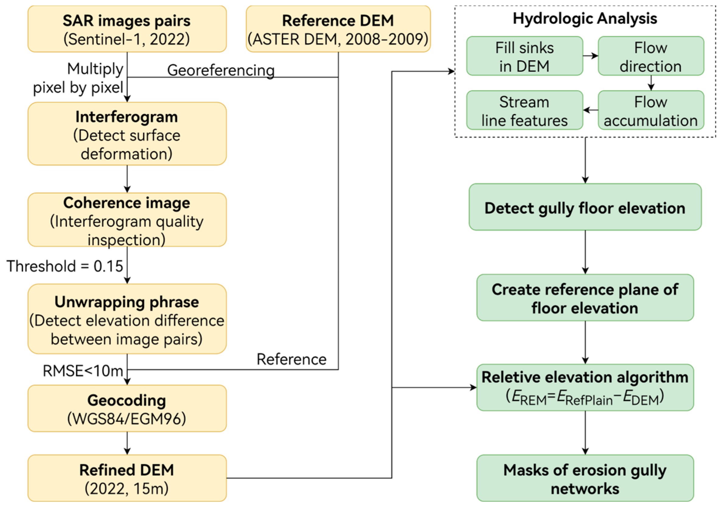
Reference ASTER GDEM V3 was downloaded from www.earthdata.nasa.gov (accessed on 10 December 2023) [42]. Version 3 of ASTER GDEM was generated using stereo data and released in 2019. According to its official user guide, the standard deviation of the elevation error has decreased to 12.1 m, an improvement compared to that of the previous versions [43]. Several studies have evaluated the accuracy of ASTER GDEM, reporting a general vertical root mean square error (RMSE) ranging from 8.52 to 30.11 m, depending on the complexity of the topography [44,45,46]. In comparison to other available DEMs such as SRTM DEM, AW3D DEM, and ALOS DEM, ASTER DEM is more suitable for assisting the phase unwrapping process in the InSAR workflow, particularly in mountainous areas [47]. Although the recently released Copernicus DEM was reported to have high accuracy [48], the central and northern regions of China have not been sufficiently observed at present [49]. Therefore, ASTER DEM was selected as a reference in this study to assist in the reconstruction of the InSAR DEM.
Landsat-9 pan-sharpened imagery was selected for manual extraction of the ground truth data of the gullies because it has a similar spatial resolution to the refined DEM. To simplify the processing workflow and focus on the main tasks of this study, we used the ©ESRI ArcGIS Online service for instant access to the preprocessed Landsat-9 imagery data (https://www.arcgis.com/home/item.html?id=a7412d0c33be4de698ad981c8ba471e6, accessed on 10 December 2023). This online platform offers a comprehensive Landsat-9 imagery collection that has been pan-sharpened and processed in a multitemporal manner. This imagery is refreshed daily using newly acquired images directly obtained from the USGS Landsat collection. It is dynamically generated in natural color with dynamic range adjustment (DRA) to facilitate visualization and analytical purposes [50]. By leveraging this online service, we efficiently accessed the prepared Landsat imagery, streamlining the complexities of traditional image processing workflows.

3. Methods

This study’s workflow comprised two stages. The initial stage involved DEM reconstruction utilizing SAR data (shown in yellow boxes in Figure 3). The ASTER DEM served as the basis for georeferencing. Selected pairs of Sentinel-1 SAR images underwent a pixel-by-pixel multiplication operation to generate an interferogram for surface deformation detection. Subsequently, a coherence image was derived from the SAR image pairs to evaluate the interferogram’s quality. Pixels with coherence values less than 0.15 were excluded. The filtered image was then subjected to phrase unwrapping and geocoding processes sequentially. Finally, the refined DEM was generated. The second stage entailed the extraction of erosion gully networks from the refined DEM (shown in green boxes in Figure 3). Hydrologic analysis was initially conducted to generate line features of streams. These features facilitated the detection of the gully floor elevation, which was used to establish the reference plane. The relative elevation algorithm was then employed to produce a relative elevation model (REM). Ultimately, the erosion gully network masks were extracted from the REM.

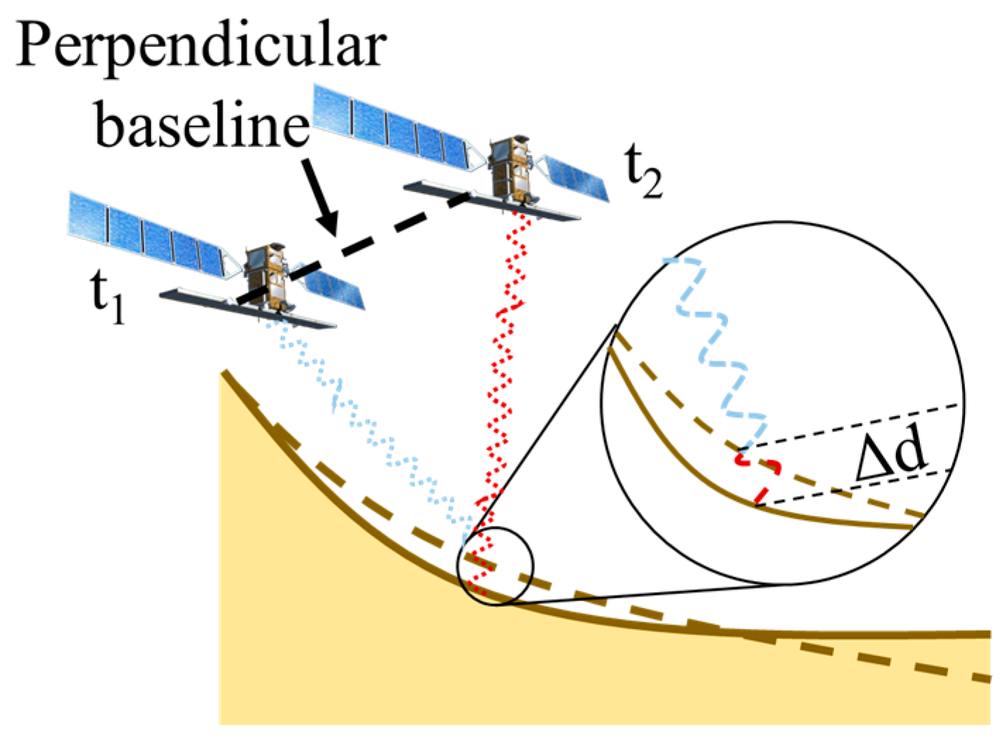
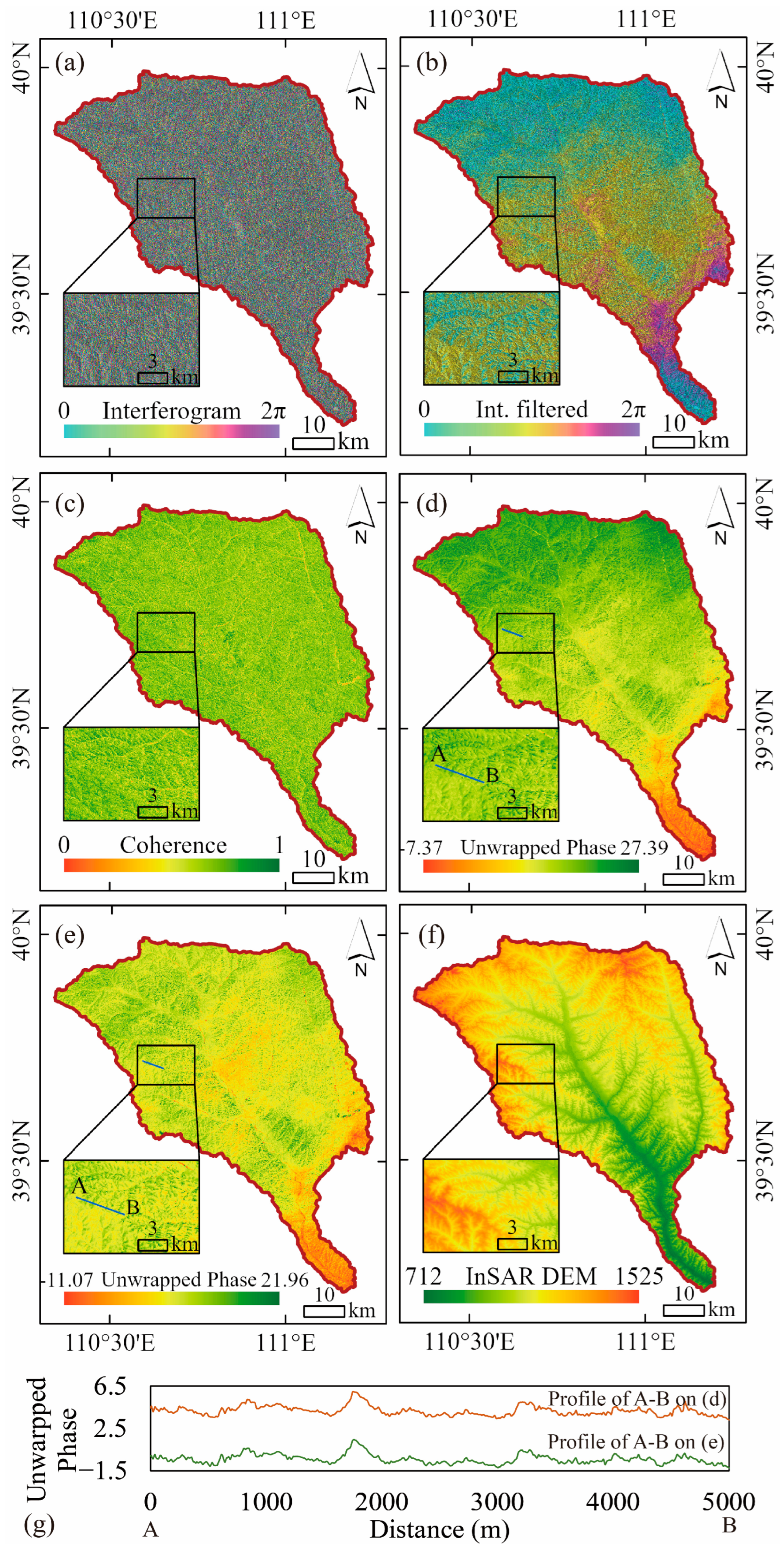
3.1. DEM Reconstruction Using SAR Data

Two different radar images with known perpendicular baselines can be used to estimate terrain information from the Earth’s surface by calculating the different path lengths of the two in-phase radar echo signals received by the antennas [51]. The varied delays of the radar echo signal received by the antennas contain the terrain change information. For example, a longer traveling time of a signal indicates it touches a concave-down surface  ( Δ d )  rather than a flat one before returning to the antenna (Figure 4). Respecting the sinusoidal nature of the radar signal, the signal ( S ) associated with time ( t ) can be expressed as in Equation (1) [52]:
S t = A cos [ 2 π f 0 ( t τ ) ] = A cos 2 π f 0 t 2 π λ 2 R
where  A  is the amplitude,  τ = 2 R c  is the time required for signals to travel back to the antenna,  λ = c f 0  is the wavelength ( c  is the speed of an electromagnetic wave), and  2 π λ 2 R  is known as the phase delay ( φ ).
Above is the original theory of InSAR, assuming that initial radar signals are sent by the antennas at the same time. However, Sentinel-1 was not designed for DEM reconstructing tasks and can only work in monostatic mode [23]. Given that the Earth’s surface does not change within a short time, repeat observations still follow the principle of InSAR so can be used to measure surface elevation [23,53]. The main steps of DEM reconstruction using Sentinel-1 data in this study are briefly explained below. Note that SAR data were processed via the SARscape 5.6 framework in ENVI 5.6 software for DEM reconstruction. For details about the processing process and intermediate results, please see Appendix A for reference.

3.1.1. Retrieving Interferogram

As mentioned above, gridded S1 images preserve the phase information about the last fraction of a complete radar wave period. To retrieve the phase information, the selected images for DEM reconstruction were cross-multiplied pixel by pixel to create an interferogram. It was a representation combining the phase variation of topography, deformation, Earth’s curvature, atmospheric effect, and noise [23]. Due to the pixel-based calculation, spatial registration must be precisely conducted in advance to obtain phase differences from the pixel pairs. In this study, we accomplished spatial registration by referencing an existing DEM for homologous image point matching.

3.1.2. Calculating Coherence Image

The coherence image between the two image was calculated to inspect the quality of the interferogram. The coherence ( γ ) is defined by its correlation coefficient as in Equation (2) [54]:
γ = E s 1 s 2 * E s 1 2 E s 2 2
where  s 1  and  s 2  represent the SAR signals captured and rasterized on the two images pair, * is the complex conjugate operator, and  E  means mathematical expectation. The value range of  γ  is  [ 0 , 1 ] . Bare land and urban areas usually have a high coherence value, while rapidly changing surfaces like water and vegetation usually have a low coherence value [23]. Signals with low coherence are unusable for DEM reconstruction. A threshold between 0.1 and 0.4 is widely accepted to filter out unusable information. Considering the number of valid pixels and the low vegetation coverage in our study area, we used 0.15 as the threshold.

3.1.3. Unwrapping Phase

The unwrapping phase can convert SAR signals from cyclic wave measurement to continuous height measurement [55]. The pixel values on an unwrapped interferogram represent topographic variation or relative height between the image pair. For proper unwrapping, we applied a Goldstein filter to the interferogram in advance to enhance the signal–noise ratio [56]. Although applying the filter may introduce errors by suppressing potential true but minor phase variations [57], the fast Fourier transformation (FFT)-based filter remains stable and functional within the usable signal range. Given the low vegetation coverage and arid climate in the study area, the benefits of this filter outweighed its drawbacks.

3.1.4. Geocoding Unwrapped Phase

Geocoding was performed to translate the unwrapped phase to metric measurement representing the true Earth’s surface height along the line between the pixel and antenna [40]. In this study, we used ASTER DEMs as the reference to rectify geometry disorders during imaging and finally retrieved reconstructed a DEM georeferenced to WGS 1984/EGM 1996.

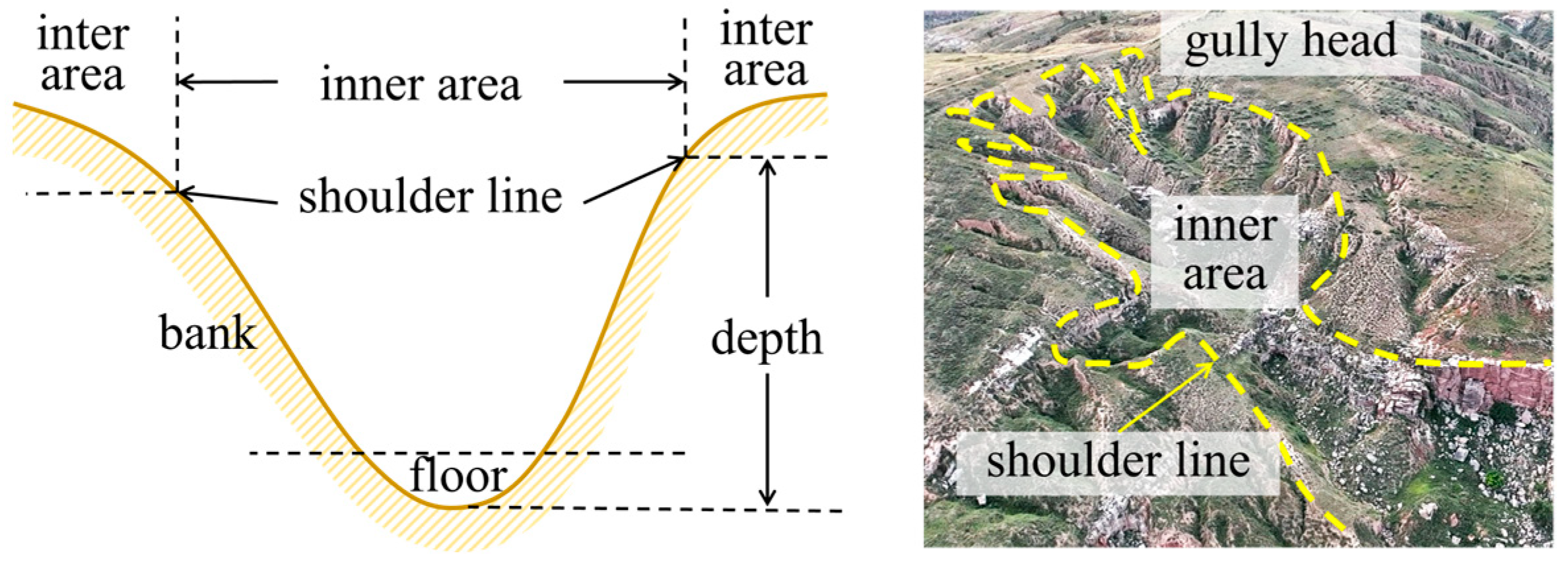
3.2. Gullies Extraction

The erosion gully refers to the inner area between shoulder lines [15], as illustrated in Figure 5. Given the close relationship between erosion gullies and streams, we introduced the following terminology from hydrology to describe a gully network: gully heads are the farthest upstream locations of gullies, junctions are the locations where two gullies join to form a downstream one, the floor is the lower part of the inner area, the bank is the part between the shoulder line and the floor, and depth is the vertical distance from the lowest point on the floor to the shoulder line.
The reconstructed DEMs were projected onto the WGS 1984 coordinate system and EGM 1996 geoid, as previously mentioned. Each DEM pixel represented the surface elevation relative to the geoid. Due to the downward-inclined nature of an erosion gully, the elevation of both the gully floor and shoulder exhibit a downward trend along the center line of erosion gullies. Thus, applying constant elevation thresholds across the landscape to extract gullies was impractical, as local elevation variations within gullies may be obscured by global terrain undulations. Drawing on the concept of the relative elevation model in cartography, we developed an REA method to eliminate the effect of global terrain. Specifically, gully floors were extended as a reference plane, and DEM elevations were vertically aligned to the reference plane. Pixel values were assigned to represent gully depths rather than absolute elevation. Consequently, the histogram distribution of these pixel values should match the topographic relief of the gullies and could help delineate inner gullies.

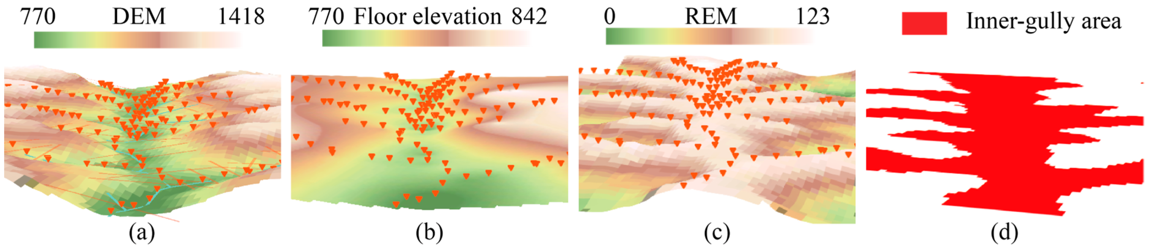
3.2.1. Detecting Floor Elevation of Erosion Gullies

The floor elevations of erosion gullies can be detected using hydrological analysis methods, as gullies are primarily shaped by hydraulic erosion. SAR-derived DEMs may contain sinks created by errors. A sink refers to a cell with an undefined drainage direction. In this study, sinks were first filled to avoid unreasonable flows. The flow direction and accumulation raster were then derived from the filled DEM using the multi-flow direction algorithm [58]. Subsequently, a stream network was generated by selecting a threshold on the flow accumulation raster. The turning point where river network density ceases to substantially increase with the threshold is often used as an optimal threshold [59]. However, to better detect small gullies, a relatively smaller threshold could be selected. As such, sampling points (orange points shown in Figure 6a) were set at equal intervals along the generated river network to extract gully floor elevations from the DEM.

3.2.2. Creating a Reference Plane

The reference plane was created by interpolating floor elevations across the study area using the ANUDEM 5.3 program built in ArcGIS Pro 3.0. ANUDEM was specifically developed to improve the interpolation of DEMs from vector inputs by adaptively managing local topographic features. It incorporates a drainage enhancement algorithm that preserves hydrological features such as streamlines and drainage structures. Additionally, it removes unnecessary kinks and generalizes the data to better manage feature conflicts [60]. In comparison to the traditional rasterizing method that utilizes the Triangular Irregular Network (TIN), significant improvements in the interpolated DEM were observed, particularly in the LP region [61]. In this study, perpendicular lines to flow direction were created at each sampling point. The length of these lines was determined by the width of the erosion gully. These lines acted as the contour lines of the reference plane, with elevation values inherited from the sampling points. Both sampling points and perpendicular lines were used as inputs of the ANUDEM program to generate the reference plane (Figure 6b).

3.2.3. Extracting Mask of Erosion Gullies Using REA

The REA is the subtraction of the elevation ( E ) of the original DEM from that of the reference plane (Equation (3)):
E R E M = E R e f P l a n e E D E M
In the REM (Figure 6c), a value of 0 corresponds to the floor of the erosion gullies, and negative values correspond to the descending height of the gully banks. After conducting the REA, the base elevation of the gully and its banks on both sides were adjusted to a consistent elevation on the reference plane. This operation standardized the base elevation of the gully, thus eliminating the downward trend. As the downward trend was removed, the undulation of the gullies was reinforced. Thus, the gullies could be extracted from the terrain using the natural breaks method. The natural breaks method was first developed for unsupervised classification in choroplethic maps [62,63]. It is a data-clustering method that minimizes elevational discrepancies within categories while maximizing those between categories. It is reported that data can be properly classified using this method, with minimal information loss [64]. The method and its variants have been successfully applied in the field of remote sensing and GIS in classification and object extraction tasks based on quantitative data [65,66,67]. After REA processing, DEM data in gully areas exhibited aggregation patterns in the gully floor and inter-gully regions. This resulted from REA normalizing the relief to a uniform base elevation, causing these two areas to share similar elevations. By applying the natural breaks method, these two categories representing the gully floor and intergully areas could be distinguished. Considering the cross-sectional characteristics of the gully, the remaining data between these two categories represented the gully bank. Converting these three categories into numeric sequences in ascending order of elevation, they, respectively, represented the gully floor, gully bank, and intergully area. Specifically, the first and second categories together represented the inner-gully area. (Figure 6d).

3.3. Validation

The ground truth mask of the gully was extracted manually from Landsat-9 pan-sharpened images at random locations within the basin. Pixels of the REA-extracted gully located in the ground truth mask were considered to be correct. Here, we applied the F1 score (Equation (4)) for validation.
F 1   s c o r e = 2 × P r e c i s i o n × R e c a l l P r e c i s i o n + R e c a l l
where  P r e c i s i o n  indicates the proportion of true positive pixels among all the positive pixels generated from the REA extraction, while  R e c a l l  indicates the proportion of true positive pixels identified using the REA extraction out of all the actual positive pixels in the ground truth. The calculation of these two indicators is given in Equations (5) and (6), respectively.
P r e c i s i o n = C o u n t T P C o u n t T P + C o u n t F P
R e c a l l = C o u n t T P C o u n t T P + C o u n t F N
where  C o u n t T P  represents the count number of true positive pixels,  C o u n t F P  represents the count number of false positive pixels, and  C o u n t F N  represents the count number of false negative pixels. The accuracy was also computed as the ratio of correctly extracted pixels to the overall pixel count for purposes of comparative analysis. This calculation is presented in Equation (7).
A c c u r a c y = C o u n t T P + C o u n t T N C o u n t T P + C o u n t F P + C o u n t T N + C o u n t F N
where  C o u n t T N  represents the count number of true negative pixels. Other parameters have the same meaning as in Equations (5) and (6). To assess the effectiveness of the method described above, it was applied again to the ASTER DEM. The validation metrics for the extracted erosion gully networks were then calculated using the same validation method to establish a reference result, which was subsequently utilized for comparative analysis.

4. Results

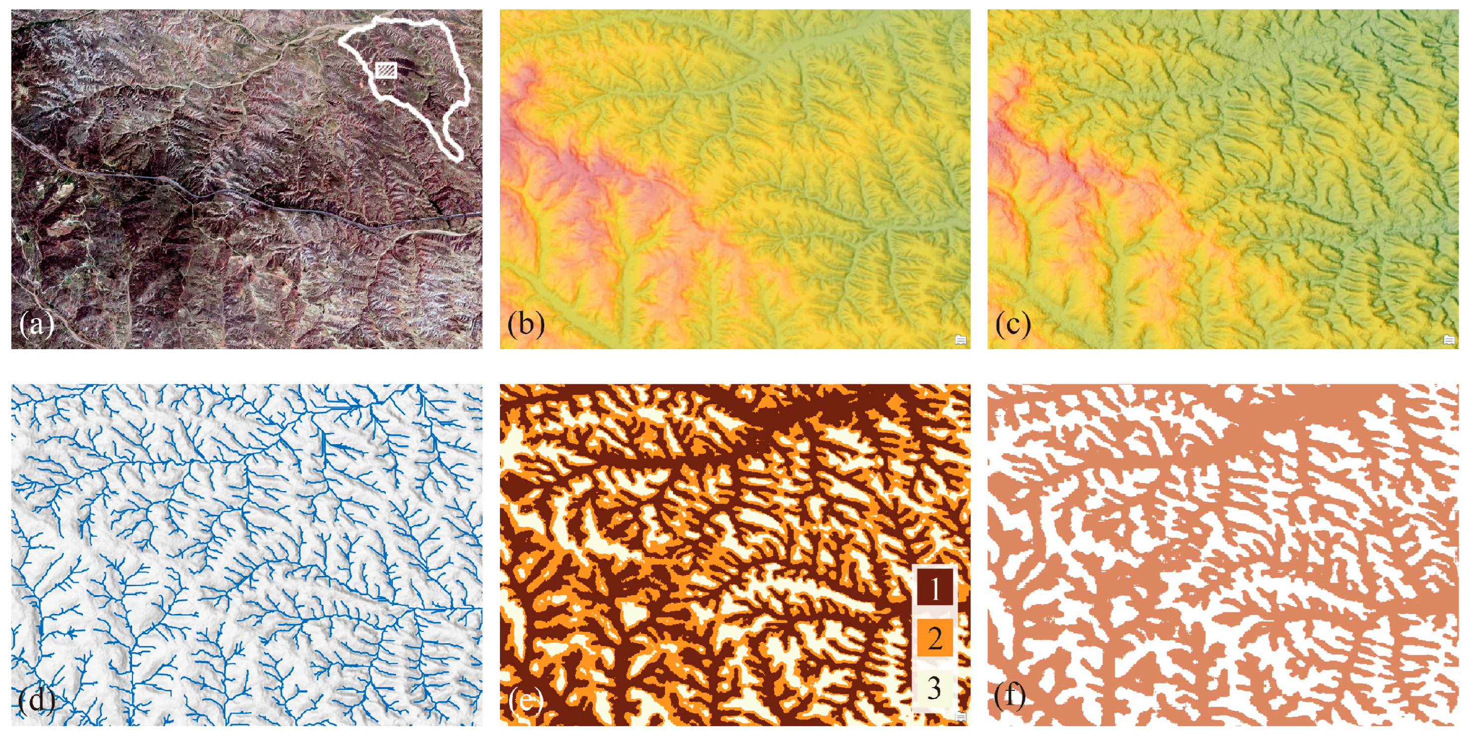
4.1. Extraction of Erosion Gullies

To demonstrate the above procedure of erosion gully extraction, we selected the HFC basin as the case region for testing. A DEM with finer spatial resolution (Figure 7c) was first reconstructed using InSAR techniques. This DEM showed enhanced terrain details with less noise compared to the reference ASTER DEM (Figure 7b). As mentioned in Section 3.2.1, a threshold of flow accumulation was determined as 100 to better detect gully heads. Tests showed that a smaller threshold could lead to the identification of stream features with lengths shorter than the sampling intervals (50 m) of floor elevation (Figure 7d). The REA was then used, and its result was classified using the natural breaks method into three parts, namely, the gully floors, the gully banks, and the intergully tablelands (Figure 7e). The initial gully mask was created by assigning null values to the pixels classified as intergully tablelands. Continuous flat areas over 1 km2 (e.g., large river channels, large tableland, etc.) were also removed using a sliding circular window with a radius of 38 pixels. The erosion gullies could finally be extracted with this optimized mask (Figure 7f).

4.2. Characteristics of Extracted Erosion Gullies

A total of 28,000 erosion gullies were identified and extracted from the HFC basin. These gullies exhibited pinnate patterns at the basin scale and trellis patterns on localized slopes (Figure 8). Using the Strahler method, the gullies were classified into five hierarchical orders. Note that the fourth- and fifth-order gullies were excluded in the following analysis because they were large river channels and were not part of this study. The results revealed that the intersecting angles at the junctions of the first- and second-, as well as second- and third-order gullies, typically exceeded 60°. Some intersecting angles in the northwestern basin reached 90°. Transverse small-watershed systems due to headward erosion were observed more commonly in this area. REA revealed that the average depth of the basin was 64 m, with 95% of the gullies ranging in depth from 50 to 78 m, and the deepest measuring 140 m.
To examine the spatial characteristics of the gullies, we calculated surface fragmentation by determining the proportion of gully planar area within a 1 km2 rectangular region. The average fragmentation was found to be 54%, indicating moderate erosive activities in the basin. The southeastern part of the basin, composed primarily of loess material, exhibited more severe surface fragmentation (over 60%) compared to the central and northwestern regions, where Pisha sandstone was predominant (Figure 9).

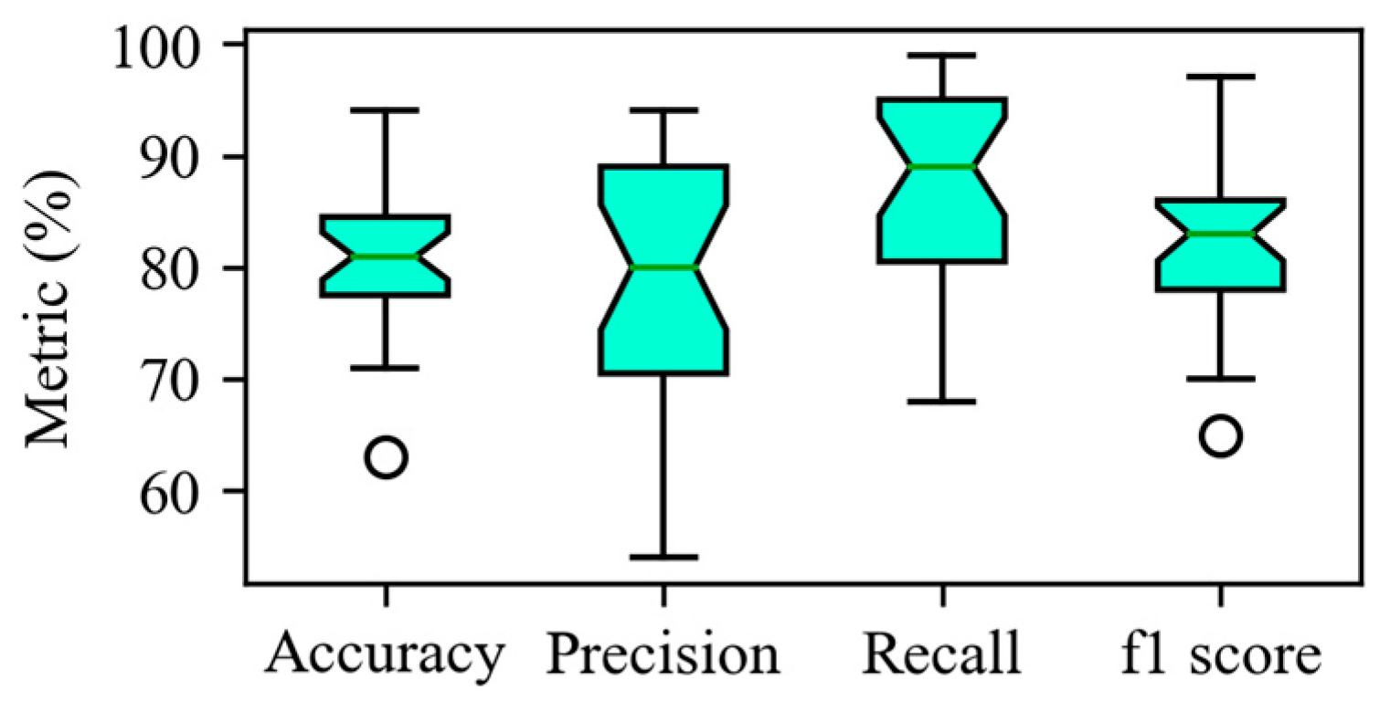
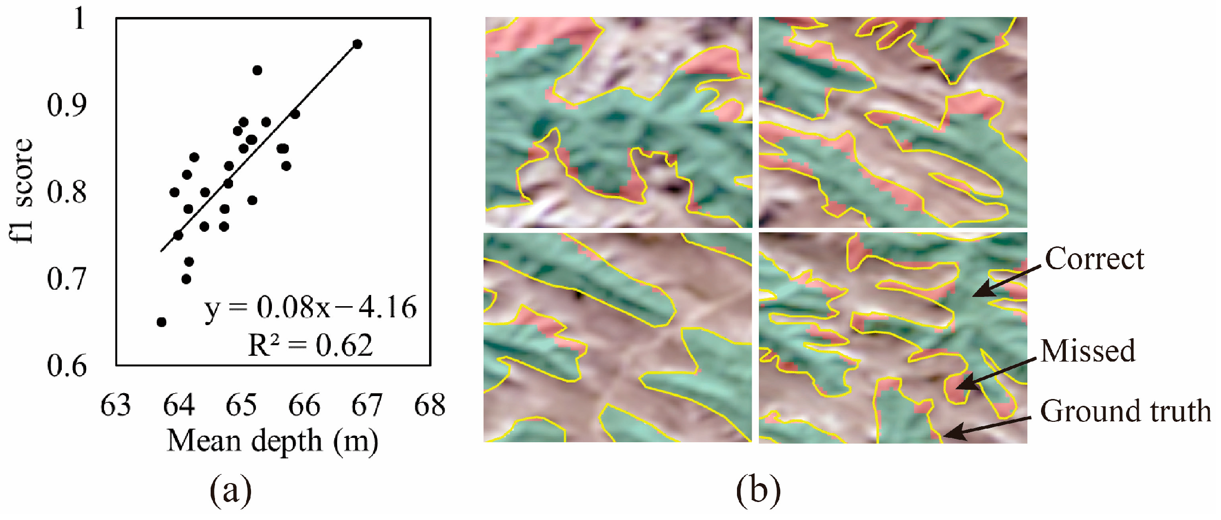
4.3. Validation of the Proposed Extraction Method

Twenty-seven square regions (1 × 1 km) within the study area were randomly selected for validation. Ground truth gully masks were manually digitalized from Landsat-9 pan-sharpened images. These images were chosen because their spatial resolution was close to that of the DEM. The accuracy, precision, recall, and F1 score of each validation region were calculated and plotted (Figure 10). The results showed that the method achieved overall good performance. It accurately identified the majority of the gullies, with an average accuracy of 80.88%. Additionally, it efficiently distinguished erosion gullies from the inner gully areas, as evidenced by the relatively high average recall of 87.76%. However, the average precision was lower than the other metrics, reaching a minimum of 54.27%. This indicates that some gullies were missed, possibly due to the coarse spatial resolution of the DEMs, which might have hindered the detection of small-scale topographic relief near the gully heads. Nonetheless, the average F1 score of 81.94% suggested that local errors did not significantly impact the overall results. The method achieved a balanced performance by effectively identifying true positives (real inner gully area) and avoiding false positives.

5. Discussion

The spatial resolution of DEMs may have significant impacts on the accuracy of gully extraction due to the resolution effect [68]. The resolution effect refers to the generalization of terrain details when using a coarser grid (lower spatial resolution) to represent the true topographic relief. It may result in a smoothed representation of the surface [69] and limits the efficiency of gully extraction. The suitable spatial resolution proposed in previous studies for gully information extraction varies from 2 m to 15 m [68,70]. For studies covering large areas, the acquisition of these high-resolution DEMs remains challenging due to their limited availability. The use of drones to obtain DEMs with high spatial resolution can also become less feasible due to time and cost issues. Nonetheless, the extraction of gullies does not necessitate a DEM with precise absolute elevation values. Because the relative elevation difference between the inner- and intergully areas is more crucial for gully extraction purposes. Thus, this study developed a method that integrates InSAR and REA techniques to facilitate rapid gully extraction over large areas. Comparative results showed that the reconstructed DEM with a finer resolution (15 m) improved gully extraction performance, with an F1 score of 81.94% for gullies’ extraction. In contrast, the reference ASTER DEM with a coarser resolution (30 m) achieved an F1 score of 72.17%. Thus, our study confirmed that it is feasible to extract gullies from lower-resolution DEMs by employing suitable information enhancement methods, as suggested by Maerker et al. [71].
Gullies in different locations may have different characteristics due to different erosion magnitudes. This can impact the accuracy of gully extraction [1]. Gully depth usually indicates the erosion rate or development age of a gully [72]. Regression analysis (Figure 11a) revealed a positive correlation between the F1 score and gully depth (R2 = 0.62), indicating that older gullies with significant elevation differences were easier to extract. Gully heads presented a higher likelihood of being missed during the extraction process, particularly when fewer than 50 continuous pixels (approximately 1 hm2) were involved (Figure 11b). Gully heads in the loess region exhibited greater fragmentation than those in the Pisha sandstone area. Indoor experiments revealed that sandy soils showed higher soil loss compared to silty soils [73]. Therefore, we could infer that the sandy-soil-dominated Pisha sandstone region was less prone to multidirectional competition at gully heads due to its high erodibility. Consequently, the degree of gully head undercutting was expected to be greater, rendering complete extraction of gullies in this region more feasible.
Future works should focus on enhancing the accuracy of gully head extraction. This can be achieved by refining the spatial resolution of the DEM or by assigning appropriate weights to the gully head area during the generation of the reference plane. This approach would emphasize the topographic gradient at the gully heads, thereby improving the accuracy of their extraction. Moreover, while this study was conducted within the context of the Loess Plateau’s erosion gullies, its applicability to other regions without distinct shoulder lines requires additional validation. Nonetheless, the method proposed here demonstrates the potential for leveraging open-source data for the rapid and extensive mapping of gully networks. The extracted gully networks provided a way to investigate gully erosion advances and geomorphology, from a systematic viewpoint.

6. Conclusions

This study integrated InSAR and REA techniques to develop a rapid method for extracting erosion gully networks. The InSAR technology reconstructed up-to-date DEMs with finer spatial resolution. And, the REA method extracted the gullies by enhancing their vertical elevation difference. The validation of the results indicated that the method achieved an F1 score of 81.94%, representing a 9.77% improvement over the reference ASTER DEM. This suggests that the application of appropriate information enhancement methods to low-resolution DEMs can be effective for gully extraction. The accuracy of the extraction was affected by the characteristics of the erosion gullies at different locations. The F1 score was positively correlated to the depth of the gullies (R2 = 0.62), while the fragmented gully heads presented a higher potential of being missed due to the resolution effect. Further insights into the erosion gully networks within the HFC basin were revealed by the extraction results. The identified 28,000 gullies in the HFC basin showed pinnate and trellis patterns. Most of the gullies had notable intersecting angles exceeding 60°. The basin’s average depth was 64 m, with the deepest gully being 140 m. Surface fragmentation indicated moderate erosive activity, with the southeastern loess region showing more severe erosion than the Pisha sandstone-dominated central and northwestern regions. In summary, the method presented in this paper offers a streamlined workflow and relatively good performance for the rapid extraction and mapping of erosion gully networks. It enables quasi-real-time monitoring of gully network development and demonstrates the potential for leveraging open-source data to rapidly map erosion gully networks at the regional scale.

Author Contributions

Conceptualization, P.L., B.Z. and X.W.; data curation, P.L., B.Z. and C.W.; formal analysis, P.L.; funding acquisition, C.W. and X.W.; investigation, P.L. and C.W.; methodology, P.L. and B.Z.; project administration, M.L. and X.W.; resources, M.L. and X.W.; software, P.L., B.Z. and M.L.; supervision, C.W., M.L. and X.W.; validation, P.L.; visualization, P.L. and B.Z.; writing—original draft, P.L.; writing—review and editing, X.W. All authors have read and agreed to the published version of the manuscript.

Funding

This study was funded by the National Natural Science Foundation of China (U2243240), the National Key R&D Program of China (2022YFE0115300, 2022YFF1300801).

Data Availability Statement

The Sentinel-1 SAR imagery and associated metadata are available on https://search.asf.alaska.edu/ (accessed on 10 December 2023). The Landsat-9 pan-sharpened tiled imagery service is provided by ©ESRI ArcGIS Online service (https://www.arcgis.com/home/item.html?id=a7412d0c33be4de698ad981c8ba471e6, accessed on 10 December 2023). The ASTER GDEM V3 is available on www.earthdata.nasa.gov (accessed on 10 December 2023).

Conflicts of Interest

The authors declare no conflicts of interest.

Appendix A

The InSAR processing details and results of the Sentinel-1 SAR image pair described in Section 3.1 are presented below for readers’ reference.
Before the InSAR workflow, the ASTER DEM was converted from EGM 1996 geoid elevation to ellipsoid elevation to match the spaceborne Sentinel-1 satellite benchmarks. In the InSAR workflow, SAR image pair ID 1 and 2 (Table 1) were designated as the master and slave images, respectively. Baseline estimation results confirmed the suitability of the image pair for interferometry (Table A1).
To address the systematic errors caused by orbit inaccuracies, precise orbit ephemerides of Sentinel-1 were used for coregistration between the image pair. Once coregistration was completed, the interferogram was generated (Figure A1a). The interferogram was then processed using the ASTER DEM as a reference to remove flat topography and adaptive filtering was applied to reduce phase noise, resulting in a flattened and filtered interferogram (Figure A1b).
Following the filtering, a coherence image was generated (Figure A1c). The result indicated good coherence in most areas of the selected SAR image pair (mean = 0.66, StdDev = 0.11). Subsequently, the unwrapping procedure was performed to obtain the absolute phase (Figure A1d).
To further reduce errors, orbit refinement, and reflattening processes were conducted, even with the application of precise orbit ephemerides. GCPs on flat topography were manually selected for this process, resulting in the generation of a reflattened unwrapped phase image (Figure A1e). The refinement achieved a root mean square error (RMSE) of 8.33, close to the priori achievable RMS of 13.01. After refinement, the mean difference and standard deviation of the GCP height were −0.23 and 5.08, respectively, indicating an improvement in the quality of the unwrapped image.
To evaluate the unwrapping process, a profile (Figure A1g) was created between points A and B (shown in the black box in Figure A1d,e). Both profiles exhibited smooth changes without significant disruptions, indicating proper unwrapping of the phase. The reflattened unwrapped phase showed a smoother trend, further indicating an improvement in the quality of the stacked phase.
Finally, the refined and reflattened unwrapped image was geocoded to WGS 1984/EGM 1996, resulting in the generation of the DEM product (Figure A1f).
Table A1. Results of baseline estimation.
ItemValue
Normal baseline (m)116.670
Critical baseline min-max−6406.247~6406.247
Range shift (pixels)−30.707
Azimuth shift (pixels)−1.836
Slant range distance (m)878,897.093
Absolute time baseline (days)24
Doppler centroid diff. (Hz)−21.058
Critical min–max (Hz)−486.486~486.486
2 PI ambiguity height (InSAR) (m)132.647
2 PI ambiguity displacement (DInSAR) (m)0.028
1 pixel shift ambiguity height (stereo radargrammetry) (m)11,142.344
1 Pixel Shift ambiguity displacement (amplitude tracking) (m)2.330
Master incidence angle39.414
Absolute incidence angle difference0.007
Figure A1. Results of the InSAR processing. (a) Interferogram; (b) adaptively filtered interferogram; (c) coherence image; (d) unwrapped image; (e) orbit refined and reflattened unwrapped image; (f) geocoded DEM production; (g) profiles of unwrapped phrase and re-flattened unwrapped phrase along the selected line A–B.
Remotesensing 16 00921 g0a1
A comparison between the InSAR refined DEM and the reference ASTER DEM was conducted by performing a subtraction operation between the two DEMs (Figure A2, left). The results showed that 61.90% of the pixels exhibited a difference below 20 m, while 38.90% had a difference ranging from 20 to 40 m. Long-term mining activities and sediment retention by check dams may have contributed to the observed variation in elevation. Elevation profiles were generated along four selected directions: AB, CD, EF, and GH (Figure A2, right). The comparison revealed that the InSAR-generated DEM exhibited higher elevations in the southern part of the study area and lower elevations in the northern part compared to the reference DEM. However, the former one captured more surface relief details. As the REA primarily focuses on relative elevation differences rather than absolute elevation accuracy, the DEM refined by InSAR can assist in capturing more details of erosion gullies in REA analysis. Additionally, the InSAR-generated DEM had a higher horizontal spatial resolution (15 m) than the reference DEM (30 m), further enhancing the performance of REA.
Figure A2. Elevation difference between InSAR refined DEM and reference ASTER DEM.
Remotesensing 16 00921 g0a2

References

  1. Zhang, C.; Wang, C.; Long, Y.; Pang, G.; Shen, H.; Wang, L.; Yang, Q. Comparative Analysis of Gully Morphology Extraction Suitability Using Unmanned Aerial Vehicle and Google Earth Imagery. Remote Sens. 2023, 15, 4302. [Google Scholar] [CrossRef]
  2. Wilkinson, S.N.; Kinsey-Henderson, A.E.; Hawdon, A.A.; Hairsine, P.B.; Bartley, R.; Baker, B. Grazing Impacts on Gully Dynamics Indicate Approaches for Gully Erosion Control in Northeast Australia. Earth Surf. Process Landf. 2018, 43, 1711–1725. [Google Scholar] [CrossRef]
  3. Ding, H.; Liu, K.; Chen, X.; Xiong, L.; Tang, G.; Qiu, F.; Strobl, J. Optimized Segmentation Based on Theweighted Aggregation Method for Loess Bank Gully Mapping. Remote Sens. 2020, 12, 793. [Google Scholar] [CrossRef]
  4. Sun, L.; Liu, Y.F.; Wang, X.; Liu, Y.; Wu, G.L. Soil Nutrient Loss by Gully Erosion on Sloping Alpine Steppe in the Northern Qinghai-Tibetan Plateau. Catena 2022, 208, 105763. [Google Scholar] [CrossRef]
  5. Vanmaercke, M.; Poesen, J.; Van Mele, B.; Demuzere, M.; Bruynseels, A.; Golosov, V.; Bezerra, J.F.R.; Bolysov, S.; Dvinskih, A.; Frankl, A.; et al. How Fast Do Gully Headcuts Retreat? Earth Sci. Rev. 2016, 154, 336–355. [Google Scholar] [CrossRef]
  6. Vanmaercke, M.; Panagos, P.; Vanwalleghem, T.; Hayas, A.; Foerster, S.; Borrelli, P.; Rossi, M.; Torri, D.; Casali, J.; Borselli, L.; et al. Measuring, Modelling and Managing Gully Erosion at Large Scales: A State of the Art. Earth Sci. Rev. 2021, 218, 103637. [Google Scholar] [CrossRef]
  7. Castillo, C.; Gómez, J.A. A Century of Gully Erosion Research: Urgency, Complexity and Study Approaches. Earth Sci. Rev. 2016, 160, 300–319. [Google Scholar] [CrossRef]
  8. Zhao, J.; Vanmaercke, M.; Chen, L.; Govers, G. Vegetation Cover and Topography Rather than Human Disturbance Control Gully Density and Sediment Production on the Chinese Loess Plateau. Geomorphology 2016, 274, 92–105. [Google Scholar] [CrossRef]
  9. Goodwin, N.R.; Armston, J.D.; Muir, J.; Stiller, I. Monitoring Gully Change: A Comparison of Airborne and Terrestrial Laser Scanning Using a Case Study from Aratula, Queensland. Geomorphology 2017, 282, 195–208. [Google Scholar] [CrossRef]
  10. Perroy, R.L.; Bookhagen, B.; Asner, G.P.; Chadwick, O.A. Comparison of Gully Erosion Estimates Using Airborne and Ground-Based LiDAR on Santa Cruz Island, California. Geomorphology 2010, 118, 288–300. [Google Scholar] [CrossRef]
  11. Liu, B.; Zhang, B.; Feng, H.; Wu, S.; Yang, J.; Zou, Y.; Siddique, K.H.M. Ephemeral Gully Recognition and Accuracy Evaluation Using Deep Learning in the Hilly and Gully Region of the Loess Plateau in China. Int. Soil. Water Conserv. Res. 2022, 10, 371–381. [Google Scholar] [CrossRef]
  12. Chen, W.; Lei, X.; Chakrabortty, R.; Chandra Pal, S.; Sahana, M.; Janizadeh, S. Evaluation of Different Boosting Ensemble Machine Learning Models and Novel Deep Learning and Boosting Framework for Head-Cut Gully Erosion Susceptibility. J. Environ. Manag. 2021, 284, 112015. [Google Scholar] [CrossRef] [PubMed]
  13. Xue, Y.; Qin, C.; Wu, B.; Zhang, G.; Fu, X.; Ma, H.; Li, D.; Wang, B. Simulation of Runoff Process Based on the 3-D River Network. J. Hydrol. 2023, 626, 130192. [Google Scholar] [CrossRef]
  14. Lv, G.N.; Qian, Y.D.; Chen, Z.M. Study of Automated Extraction of Shoulder Line of Valley from Grid Digital Elevation Data. Sci. Geogr. Sin. 1998, 18, 567–573. [Google Scholar]
  15. Yan, S.; Tang, G.; Li, F.; Zhang, L. Snake Model for the Extraction of Loess Shoulder-Line from DEMs. J. Mt. Sci. 2014, 11, 1552–1559. [Google Scholar] [CrossRef]
  16. Yan, S.; Tang, G.; Li, F.; Dong, Y. An Edge Detection Based Method for Extraction of Loess Shoulder-Line from Grid DEM. Geomat. Inf. Sci. Wuhan Univ. 2011, 36, 363–367. [Google Scholar]
  17. Jiang, S.; Tang, G.; Liu, K. A New Extraction Method of Loess Shoulder-Line Based on Marr-Hildreth Operator and Terrain Mask. PLoS ONE 2015, 10, e0123804. [Google Scholar] [CrossRef]
  18. Yang, X.; Na, J.; Tang, G.; Wang, T.; Zhu, A. Bank Gully Extraction from DEMs Utilizing the Geomorphologic Features of a Loess Hilly Area in China. Front. Earth Sci. 2019, 13, 151–168. [Google Scholar] [CrossRef]
  19. Poesen, J.; Nachtergaele, J.; Verstraeten, G.; Valentin, C. Gully Erosion and Environmental Change: Importance and Research Needs. Catena 2003, 50, 91–133. [Google Scholar] [CrossRef]
  20. Qin, F.; Han, Z. Landform Evolution Modeling of a Small Catchment in the Loess Plateau. In Proceedings of the 2010 18th International Conference on Geoinformatics, Beijing, China, 18–20 June 2010; pp. 1–8. [Google Scholar]
  21. Zhang, W.; Zhu, W.; Tian, X.; Zhang, Q.; Zhao, C.; Niu, Y.; Wang, C. Improved DEM Reconstruction Method Based on Multibaseline InSAR. IEEE Geosci. Remote Sens. Lett. 2022, 19, 4011505. [Google Scholar] [CrossRef]
  22. Liu, S.; Tang, H.; Feng, Y.; Chen, Y.; Lei, Z.; Wang, J.; Tong, X. A Comparative Study of DEM Reconstruction Using the Single-Baseline and Multibaseline InSAR Techniques. IEEE J. Sel. Top. Appl. Earth Obs. Remote Sens. 2021, 14, 8512–8521. [Google Scholar] [CrossRef]
  23. Braun, A. Retrieval of Digital Elevation Models from Sentinel-1 Radar Data—Open Applications, Techniques, and Limitations. Open Geosci. 2021, 13, 532–569. [Google Scholar] [CrossRef]
  24. Zhou, X.; Chang, N.-B.; Li, S. Applications of SAR Interferometry in Earth and Environmental Science Research. Sensors 2009, 9, 1876–1912. [Google Scholar] [CrossRef]
  25. Hu, J.; Li, Z.W.; Ding, X.L.; Zhu, J.J.; Zhang, L.; Sun, Q. Resolving Three-Dimensional Surface Displacements from InSAR Measurements: A Review. Earth Sci. Rev. 2014, 133, 1–17. [Google Scholar] [CrossRef]
  26. Berardino, P.; Fornaro, G.; Lanari, R.; Sansosti, E. A New Algorithm for Surface Deformation Monitoring Based on Small Baseline Differential SAR Interferograms. IEEE Trans. Geosci. Remote Sens. 2002, 40, 2375–2383. [Google Scholar] [CrossRef]
  27. Zhao, C.; Zhang, Q.; He, Y.; Peng, J.; Yang, C.; Kang, Y. Small-Scale Loess Landslide Monitoring with Small Baseline Subsets Interferometric Synthetic Aperture Radar Technique—Case Study of Xingyuan Landslide, Shaanxi, China. J. Appl. Remote Sens. 2016, 10, 026030. [Google Scholar] [CrossRef]
  28. Olson, P.L.; Legg, N.T.; Abbe, T.B.; Reinhart, M.A.; Radloff, J.K. A Methodology for Delineating Planning-Level Channel Migration Zones; Washington State Department of Ecology Publication: Washington, DC, USA, 2014.
  29. Fu, B. Soil Erosion and Its Control in the Loess Plateau of China. Soil. Use Manag. 1989, 5, 76–82. [Google Scholar] [CrossRef]
  30. Zhang, Y.; He, Y.; Song, J. Effects of Climate Change and Land Use on Runoff in the Huangfuchuan Basin, China. J. Hydrol. 2023, 626, 130195. [Google Scholar] [CrossRef]
  31. Sui, J.; He, Y.; Karney, B.W. Flow and High Sediment Yield from the Huangfuchuan Watershed. Int. J. Environ. Sci. Technol. 2008, 5, 149–160. [Google Scholar] [CrossRef]
  32. Dang, S.; Liu, X.; Yin, H.; Guo, X. Prediction of Sediment Yield in the Middle Reaches of the Yellow River Basin Under Extreme Precipitation. Front. Earth Sci. 2020, 8, 542686. [Google Scholar] [CrossRef]
  33. Shi, H.; Li, T.; Wang, K.; Zhang, A.; Wang, G.; Fu, X. Physically Based Simulation of the Streamflow Decrease Caused by Sediment-trapping Dams in the Middle Yellow River. Hydrol. Process 2016, 30, 783–794. [Google Scholar] [CrossRef]
  34. Ma, W.; Tang, P.; Zhou, X.; Li, G.; Zhu, W. Study on the Failure Mechanism of a Modified Hydrophilic Polyurethane Material Pisha Sandstone System under Dry–Wet Cycles. Polymers 2022, 14, 4837. [Google Scholar] [CrossRef]
  35. Li, C.; Song, L.; Cao, Y.; Zhao, S.; Liu, H.; Yang, C.; Cheng, H.; Jia, D. Investigating the Mechanical Property and Enhanced Mechanism of Modified Pisha Sandstone Geopolymer via Ion Exchange Solidification. Gels 2022, 8, 300. [Google Scholar] [CrossRef]
  36. Zhang, X.; Li, X.; Lu, Y.; Lu, Y.; Fan, W. A Study on the Collapse Characteristics of Loess Based on Energy Spectrum Superposition Method. Heliyon 2023, 9, e18643. [Google Scholar] [CrossRef]
  37. Chen, H.; Jiang, Y.; Gao, Y.; Yuan, X. Structural Characteristics and Its Influencing Factors of Typical Loess. Bull. Eng. Geol. Environ. 2019, 78, 4893–4905. [Google Scholar] [CrossRef]
  38. Liang, Z.; Wu, Z.; Yao, W.; Noori, M.; Yang, C.; Xiao, P.; Leng, Y.; Deng, L. Pisha Sandstone: Causes, Processes and Erosion Options for Its Control and Prospects. Int. Soil. Water Conserv. Res. 2019, 7, 1–8. [Google Scholar] [CrossRef]
  39. Zhang, K.; Xu, M.; Wang, Z. Study on Reforestation with Seabuckthorn in the Pisha Sandstone Area. J. Hydro-Environ. Res. 2009, 3, 77–84. [Google Scholar] [CrossRef]
  40. Alessandro, F.; Andrea, M.-G.; Claudio, P.; Fabio, R.; Didier, M. Part A: Interferometric SAR Image Processing and Interpretation. In InSAR Principles: Guidelines for SAR Interferometry Processing and Interpretation; Karen, F., Ed.; ESA Publications: Noordwijk, The Netherlands, 2007. [Google Scholar]
  41. National Aeronautics and Space Administration (NASA) Sentinel-1—Alaska Satellite Facility. Available online: https://asf.alaska.edu/datasets/daac/sentinel-1/ (accessed on 10 December 2023).
  42. NASA/METI/AIST/Japan Space Systems and U.S./Japan ASTER Science Team. ASTER Global Digital Elevation Model V003. Available online: https://lpdaac.usgs.gov/products/astgtmv003/ (accessed on 10 December 2023).
  43. Michael, A.; Robert, C. ASTER GDEM V3 (ASTER Global DEM) User Guide. Available online: https://lpdaac.usgs.gov/documents/434/ASTGTM_User_Guide_V3.pdf (accessed on 10 December 2023).
  44. Liu, X.; Ran, M.; Xia, H.; Deng, M. Evaluating Vertical Accuracies of Open-Source Digital Elevation Models over Multiple Sites in China Using GPS Control Points. Remote Sens. 2022, 14, 2000. [Google Scholar] [CrossRef]
  45. Gesch, D.; Oimoen, M.; Danielson, J.; Meyer, D. Validation of the ASTER Global Digital Elevation Model Version 3 over the Conterminous United States. Int. Arch. Photogramm. Remote Sens. Spat. Inf. Sci. 2016, XLI-B4, 143–148. [Google Scholar] [CrossRef]
  46. Sun, L.; Liu, P.; Zhang, W.; Hou, S.; Sun, H. Precision Comparing and Analyzing Between ASTER DEM and 1:50000 National Digital Elevation Data. Geomat. Spat. Inf. Technol. 2013, 36, 1–6. [Google Scholar]
  47. Liu, H.; Zhou, B.; Bai, Z.; Zhao, W.; Zhu, M.; Zheng, K.; Yang, S.; Li, G. Applicability Assessment of Multi-Source DEM-Assisted InSAR Deformation Monitoring Considering Two Topographical Features. Land 2023, 12, 1284. [Google Scholar] [CrossRef]
  48. Li, H.; Zhao, J.; Yan, B.; Yue, L.; Wang, L. Global DEMs Vary from One to Another: An Evaluation of Newly Released Copernicus, NASA and AW3D30 DEM on Selected Terrains of China Using ICESat-2 Altimetry Data. Int. J. Digit. Earth 2022, 15, 1149–1168. [Google Scholar] [CrossRef]
  49. Vera, L.-T.; Philipp, J.; Henning, S.; Hanjo, K. Copernicus DEM Copernicus Digital Elevation Model Validation Report. Available online: https://spacedata.copernicus.eu/documents/20123/121239/GEO1988-CopernicusDEM-RP-001_ValidationReport_I3.0.pdf/ (accessed on 10 December 2023).
  50. Esri. Pansharpened Landsat. Available online: https://www.arcgis.com/home/item.html?id=a7412d0c33be4de698ad981c8ba471e6 (accessed on 10 December 2023).
  51. Zebker, H.A.; Goldstein, R.M. Topographic Mapping from Interferometric Synthetic Aperture Radar Observations. J. Geophys. Res. Solid. Earth 1986, 91, 4993–4999. [Google Scholar] [CrossRef]
  52. Uys, D. InSAR: An Introduction. Preview 2016, 2016, 43–48. [Google Scholar] [CrossRef]
  53. Hanssen, R.F. Radar Interferometry: Data Interpretation and Error Analysis; Kluwer Academic Publishers: Dordrecht, The Netherlands, 2001. [Google Scholar]
  54. Wang, T.; Liao, M.; Perissin, D. InSAR Coherence-Decomposition Analysis. IEEE Geosci. Remote Sens. Lett. 2010, 7, 156–160. [Google Scholar] [CrossRef]
  55. Zebker, H.A.; Lu, Y. Phase Unwrapping Algorithms for Radar Interferometry: Residue-Cut, Least-Squares, and Synthesis Algorithms. J. Opt. Soc. Am. A 1998, 15, 586. [Google Scholar] [CrossRef]
  56. Goldstein, R.M.; Werner, C.L. Radar Interferogram Filtering for Geophysical Applications. Geophys. Res. Lett. 1998, 25, 4035–4038. [Google Scholar] [CrossRef]
  57. Kervyn, F. Modelling Topography with SAR Interferometry: Illustrations of a Favourable and Less Favourable Environment. Comput. Geosci. 2001, 27, 1039–1050. [Google Scholar] [CrossRef]
  58. Qin, C.; Zhu, A.-X.; Pei, T.; Li, B.; Zhou, C.; Yang, L. An Adaptive Approach to Selecting a Flow-partition Exponent for a Multiple-flow-direction Algorithm. Int. J. Geogr. Inf. Sci. 2007, 21, 443–458. [Google Scholar] [CrossRef]
  59. Zhang, H.; Loáiciga, H.A.; Feng, L.; He, J.; Du, Q. Setting the Flow Accumulation Threshold Based on Environmental and Morphologic Features to Extract River Networks from Digital Elevation Models. ISPRS Int. J. Geoinf. 2021, 10, 186. [Google Scholar] [CrossRef]
  60. Hutchinson, M.F.; Xu, T.; Stein, J. Recent Progress in the ANUDEM Elevation Gridding Procedure. 2011. Available online: https://www.researchgate.net/publication/268405980_Recent_Progress_in_the_ANUDEM_Elevation_Gridding_Procedure (accessed on 10 December 2023).
  61. Yang, Q.; McVicar, T.R.; Van Niel, T.G.; Hutchinson, M.F.; Li, L.; Zhang, X. Improving a Digital Elevation Model by Reducing Source Data Errors and Optimising Interpolation Algorithm Parameters: An Example in the Loess Plateau, China. Int. J. Appl. Earth Obs. Geoinf. 2007, 9, 235–246. [Google Scholar] [CrossRef]
  62. Jenks, G.F.; Caspall, F.C. Error on Choroplethic Maps: Definition, Measurement, Reduction. Ann. Assoc. Am. Geogr. 1971, 61, 217–244. [Google Scholar] [CrossRef]
  63. Jenks, G.F. The Data Model Concept in Statistical Mapping. Int. Yearb. Cartogr. 1967, 7, 186–190. [Google Scholar]
  64. Osaragi, T. Classification Methods for Spatial Data Representation. In Osaragi, Toshihiro (2002) Classification Methods for Spatial Data Representation; Working paper. CASA Working Papers (40); Centre for Advanced Spatial Analysis (UCL): London, UK, 2008. [Google Scholar]
  65. Hou, C.; Xie, Y.; Zhang, Z. An Improved Convolutional Neural Network Based Indoor Localization by Using Jenks Natural Breaks Algorithm. China Commun. 2022, 19, 291–301. [Google Scholar] [CrossRef]
  66. Anchang, J.Y.; Ananga, E.O.; Pu, R. An Efficient Unsupervised Index Based Approach for Mapping Urban Vegetation from IKONOS Imagery. Int. J. Appl. Earth Obs. Geoinf. 2016, 50, 211–220. [Google Scholar] [CrossRef]
  67. Su, H.; Ma, X.; Li, M. An Improved Spatio-Temporal Clustering Method for Extracting Fire Footprints Based on MCD64A1 in the Daxing’anling Area of North-Eastern China. Int. J. Wildland Fire 2023, 32, 679–693. [Google Scholar] [CrossRef]
  68. Dai, W.; Yang, X.; Na, J.; Li, J.; Brus, D.; Xiong, L.; Tang, G.; Huang, X. Effects of DEM Resolution on the Accuracy of Gully Maps in Loess Hilly Areas. Catena 2019, 177, 114–125. [Google Scholar] [CrossRef]
  69. Thompson, J.A.; Bell, J.C.; Butler, C.A. Digital Elevation Model Resolution: Effects on Terrain Attribute Calculation and Quantitative Soil-Landscape Modeling. Geoderma 2001, 100, 67–89. [Google Scholar] [CrossRef]
  70. Salekin, S.; Lad, P.; Morgenroth, J.; Dickinson, Y.; Meason, D.F. Uncertainty in Primary and Secondary Topographic Attributes Caused by Digital Elevation Model Spatial Resolution. Catena 2023, 231, 107320. [Google Scholar] [CrossRef]
  71. Maerker, M.; Quénéhervé, G.; Bachofer, F.; Mori, S. A Simple DEM Assessment Procedure for Gully System Analysis in the Lake Manyara Area, Northern Tanzania. Nat. Hazards 2015, 79, 235–253. [Google Scholar] [CrossRef]
  72. Ghosh, S.; Guchhait, S.K.; Illahi, R.A.; Bera, S.; Roy, S. Geomorphic Character and Dynamics of Gully Morphology, Erosion and Management in Laterite Terrain: Few Observations from Dwarka—Brahmani Interfluve, Eastern India. Geol. Ecol. Landsc. 2022, 6, 188–216. [Google Scholar] [CrossRef]
  73. Wang, R.; Li, P.; Li, Z.; Yu, K.; Han, J.; Zhu, Y.; Su, Y. Effects of Gully Head Height and Soil Texture on Gully Headcut Erosion in the Loess Plateau of China. Catena 2021, 207, 105674. [Google Scholar] [CrossRef]
Figure 1. Photos of typical landforms in the Huangfuchuan Basin (photographed in August 2023). (a) panorama photo showing the landforms; (b) a photo of a typical erosion gully; (c) a photo of a typical erosion gully head.
Remotesensing 16 00921 g001
Figure 2. The geographic location of the Huangfuchuan River basin.
Remotesensing 16 00921 g002
Figure 3. Flow chart of the workflow in this study.
Remotesensing 16 00921 g003
Figure 4. Theory of SAR interferometry. The blue and red dashed lines are conceptual illustrations of the signals sent by the satellite at different positions.
Remotesensing 16 00921 g004
Figure 5. Illustration of inner gully area and relative terminology used in this study.
Remotesensing 16 00921 g005
Figure 6. Three-dimensional views for illustrating the process of the relative elevation algorithm (REA). (a) DEM: orange triangular dots and lines represented the sampling points of elevation and the perpendicular lines, respectively; (b) generated reference plane; (c) REA-generated relative elevation model; and (d) extracted gullies.
Remotesensing 16 00921 g006
Figure 7. Erosion gully extraction procedures (in a demonstration area to better show the details). (a) Satellite imagery for visual support, the upper right map indicates the location of this demonstration area in the basin; (b) reference DEM; (c) reconstructed DEM; (d) streams for elevation detection; (e) reclassified REM, 1 = gully floors, 2 = gully banks, and 3 = inter-gully area; (f) extracted mask of the erosion gullies.
Remotesensing 16 00921 g007
Figure 8. Spatial patterns and gully depths of the erosion gullies in the HFC basin.
Remotesensing 16 00921 g008
Figure 9. Surface fragmentation of the HFC basin.
Remotesensing 16 00921 g009
Figure 10. Extraction validation results at 27 randomly selected regions within the HFC basin.
Remotesensing 16 00921 g010
Figure 11. Impacts of gully characteristics on extraction accuracy. (a) Regression analysis between F1 scores and mean depths of the erosion gullies; (b) extraction performance at gully head locations.
Remotesensing 16 00921 g011
Table 1. SAR data details.
IDAcquired TimePathFrameBeam ModePolarizationBaseline
Perpendicular (m)Temporal (d)
124 November 2022 10:30:34113126IWVV + VH12724
218 November 2022 10:30:33113126IWVV + VH
Disclaimer/Publisher’s Note: The statements, opinions and data contained in all publications are solely those of the individual author(s) and contributor(s) and not of MDPI and/or the editor(s). MDPI and/or the editor(s) disclaim responsibility for any injury to people or property resulting from any ideas, methods, instructions or products referred to in the content.

