1. Introduction
As numerical weather prediction (NWP) models progress, refining the initial field remains a central focus in improving the accuracy of numerical simulations [
1]. Meteorological satellite data, with its continuous observations and unrestricted geographical coverage, has become indispensable for assimilation into numerical models to improve the precision of initial fields. In recent years, assimilating various types of satellite data to improve the initial field accuracy has become a major direction in NWP research. Among these, infrared hyperspectral satellite data, due to their high temporal and spectral resolution, stand out as vital observational data for enhancing global models [
2]. Many studies have assimilated infrared hyperspectral data into global and regional models, demonstrating significant improvements in forecast applications. In its early stages, the assimilation of infrared hyperspectral data primarily focused on retrieving temperature and humidity profile data [
3,
4,
5,
6]. With the evolution of rapid radiative transfer models, there has been an increasing utilization of directly assimilating satellite-observed radiances into numerical models, such as the National Centers for Environmental Prediction (NCEP) in the United States and the European Centre for Medium-Range Weather Forecasts (ECMWF) in Europe [
7]. ECMWF initiated the operational assimilation of AIRS radiances in 2003 [
8]. Le Marshall et al. demonstrated the influence of assimilating AIRS (atmospheric infrared sounder) radiances into the NCEP global model, showing favorable outcomes in model performance [
9].
With the increasing deployment of infrared hyperspectral instruments on satellites, there is a growing application of infrared hyperspectral data from instruments such as the AIRS, the Infrared Atmospheric Sounding Interferometer (IASI) on MetOp (Meteorological Operational) satellites, and the Cross-track Infrared Sounder (CrIS) on NOAA Series satellites. Moreover, China’s FengYun-3 (FY-3) satellites are equipped with the Hyperspectral Infrared Atmospheric Sounder (HIRAS), while the FengYun-4 (FY-4) satellites feature the Geostationary Interferometric Infrared Sounder (GIIRS).
IASI data have been assimilated operationally by ECMWF, and have shown a substantial positive impact on forecasts [
10]. The French Meteorological Office introduced IASI data into its global model in July 2008, demonstrating that assimilating IASI clear-sky radiances significantly enhances global model forecast skills [
11]. Collard et al. highlighted various challenges in assimilating infrared hyperspectral IASI, such as the increased utilization of cloud-contaminated data [
12]. Joo et al. conducted a comprehensive analysis of the application of different observation types used in the UK Met Office operational assimilation system, affirming the high value of infrared hyperspectral IASI on the MetOp-A satellite [
13]. Li Gang et al. (2016) performed a one-month bias correction study for IASI long-wave CO
2 channels within China’s Global/Regional Assimilation and Prediction System (GRAPES), revealing effective corrections in the mid-to-upper levels but inadequate feedback due to insufficient data samples in the lower levels caused by cloud contamination [
14]. Yin R. et al. (2021) demonstrated improvements in the global model by assimilating FY-4 GIIRS infrared spectral data within China’s GRAPES model [
15].
In addition to its application to global models, infrared hyperspectral data have also played an important role in regional models. Xu et al. (2013) assimilated IASI data within the WRFDA (Weather Research and Forecasting Data Assimilation) system, enhancing the forecast accuracy of tropical cyclones in the regional models [
16]. Lim et al. (2014) employed clear-sky radiance data from AIRS within a regional model [
17].
In previous studies, data from polar-orbiting satellites such as AIRS, IASI, CRIS, and HIRAS were primarily obtained from morning and afternoon orbits. However, on 5 July 2021, China launched its first FY-3E meteorological satellite in a dawn–dusk orbit, capable of capturing infrared hyperspectral data during both early morning and evening passes. This satellite effectively fills observation gaps in polar-orbiting satellite coverage, complementing morning and afternoon data to create a six-times-daily global observation cycle. This advancement is expected to play a crucial role in numerical weather prediction.
Therefore, in this paper, our primary objective is to conduct an assimilation diagnosis of the FY-3E HIRAS hyperspectral infrared radiation data within the global model. This analysis aims to enhance our understanding of the added value of the FY-3E HIRAS data and its impact on improving assimilation within the global model for more accurate weather forecasts.
This paper is structured as follows:
Section 2 outlines the FY-3E HIRAS satellite observations, providing an overview of the China Meteorological Administration Global Forecast System (CMA-GFS) model, and detailing the Advanced Radiative Transfer Modeling System (ARMS) observation operator.
Section 3 elaborates on the pre-processing methods for cloud detection, quality control, bias correction, and other relevant data treatments.
Section 4 investigates the influence on the analysis field of CMA-GFS during the assimilation of FY-3E HIRAS radiances.
Section 5 assesses the impact on atmospheric parameter forecasting by comparing the results with and without assimilating FY-3E HIRAS radiances data. Finally,
Section 6 offers the research conclusions drawn from the study.
2. Data and Models
2.1. FY-3E HIRAS Data
The FY-3E HIRAS is a payload deployed on the world’s first polar-orbiting meteorological satellite in a dawn–dusk orbit and its equator crossing time (ECT) is about 5:30 a.m. [
18]. Since its launch in July 2021, FY-3E has bridged the observation gap during the polar-orbiting satellite’s dawn and dusk periods. This accomplishment ensures comprehensive global satellite data coverage with 4 h intervals through a coordinated observation network of polar-orbiting satellites. Furthermore, it has facilitated China’s numerical forecast models to achieve 100% global coverage for satellite data within a six-hour assimilation window period. The application of FY-3E satellite data holds paramount significance in refining the global Earth observation system and enhancing the efficacy of data application in NWP model.
The FY-3E HIRAS is a step-scanning Fourier transform spectrometer characterized by high spectral resolution. Its vertical spectral resolution is 0.625 cm
−1, covering a range from 648.75 to 2551.25 cm
−1 across a total of 3053 channels. This instrument operates across three spectral bands: long-wave infrared (LWIR: 648.75 cm
−1–1169.375 cm
−1), medium-wave infrared (MWIR: 1167.5 cm
−1–1921.25 cm
−1), and short-wave infrared (SWIR: 1919.375 cm
−1–2551.25 cm
−1), employing a 9 (3 × 3)-element small-scale array detectors across the bands observing nine distinct target regions on the Earth’s surface simultaneously. For each pixel having a field of view (FOV) angle of 1°, its ground scan angle spans from −50.4° to 50.4°, and it is divided into 28 fixed fields of regard (FOR). Correspondingly, the ground footprint diameter at the nadir point is approximately 14 km. The NE∆T (noise equivalent differential temperature) varies from 0.8 K to 0.2 K from longer to shorter wavelengths band before apodization, respectively (
https://space.oscar.wmo.int/instruments/view/hiras_2, accessed on 9 November 2023) [
19,
20].
Table 1 shows the specific instrument parameters.
FY-3E HIRAS furnishes temperature and humidity information across different atmospheric layers, offering invaluable data for numerical models. Leveraging its high spectral characteristics and the advantages of the dawn–dusk orbit, FY-3E HIRAS holds a pivotal position in enhancing numerical weather prediction applications.
This study utilized the L1 operational data from FY-3E HIRAS which has undergone extensive preprocessing and spectral radiance calibration. Prior research has indicated the favorable accuracy in the calibration and positioning of FY-3E HIRAS data, with overall stable brightness temperature biases [
21,
22]. These findings affirm the suitability of FY-3E HIRAS data for assimilation and numerical weather prediction applications.
2.2. CMA-GFS Global Four-Dimensional Variational Data Assimilation System
This study employed the new-generation CMA-GFS (China Meteorological Administration—Global Forecast System) global model, autonomously developed by the China Meteorological Administration [
23]. Initially known as GRAPES-GFS, it was renamed CMA-GFS in 2022. This research utilized the upgraded version CMA-GFS 4.0 which was implemented in 2023. The model features a horizontal resolution of 25 km, comprising 87 vertical layers with the model top at 0.1 hPa. Its core technologies encompass a four-dimensional variational assimilation system, a semi-implicit semi-Lagrangian fully compressible non-hydrostatic dynamic core, and a modular configuration for flexible physical process schemes. CMA-GFS incorporates various physical process schemes such as long- and short-wave radiation schemes from the rapid radiative transfer model (RRTMG) [
24], CoLM (common land model) land surface scheme [
25], the medium-range forecast (MRF) planetary boundary layer scheme [
26], the new simplified Arakawa–Schubert (NSAS) cumulus convection parameterization schemes [
27,
28,
29], the explicitly prognostic cloud cover schemes [
30], the CMA double-moment microphysics scheme, and the macrophysics cloud condensation schemes [
31,
32,
33]. Previous research work proved the satisfactory performance of CMA-GFS in operational use [
34,
35].
CMA-GFS initially utilized the 3DVAR (three-dimensional variational data assimilation system) assimilation method, later upgrading to 4DVAR in 2019. The 4DVAR implementation in CMA-GFS incorporates the incremental analysis update scheme [
36]. Compared to 3DVAR, the 4DVAR system effectively assimilates 50% more observational data, leading to a significant reduction in analysis and forecast error amplitudes [
37]. The assimilation window for CMA-GFS 4DVAR spans six hours. The assimilated data in this study encompass both conventional observations and satellite data sources.
2.3. ARMS Operational Operator
The satellite observation data, distinct from conventional observations, do not act as a model variable, and exhibit nonlinear correlations with model variables like temperature and humidity. Leveraging radiative transfer models, satellite radiances are directly assimilated into the model, in order to avoid the complex observational error propagations during the inversion assimilation. In the CMA-GFS 4DVAR assimilation system, we used the advanced radiative transfer modeling system (ARMS) which was developed in CMA for satellite data assimilation and remote sensing applications. It has capabilities from fast radiative transfer models utilized in US and European satellite programs but focuses on radiative transfer components that are essential for assimilating FengYun satellite data and sensors absent in existing models. ARMS simulations have been rigorously compared with other models and FengYun satellite observations, demonstrating strong alignment between the ARMS outputs and existing fast radiative transfer models. This substantiates ARMS’ robust simulation capabilities, especially in accommodating various existing satellite sensors [
38,
39,
40].
3. FY-3E HIRAS Data Assimilation
3.1. Data Preparation
Before assimilation, the FY-3E HIRAS data passed through a quality-control stage including bias correction, cloud detection, apodization, and other checks to insure that the observation is suitable for assimilation in the 4D-Var system.
Aligned with methodologies for other satellite radiance data in CMA-GFS, a bias correction scheme introduced by Harris and Kelly [
41] is employed. It consists of an air-mass bias correction and a scan bias correction. Three model predictors are used for air-mass bias correction, namely the 1000–300 hpa thickness, 200–50 hPa thickness, and 50–10 hPa thickness, to correct the FY-3E HIRAS data.
For cloud detection, the clear channel scheme presented by McNally and Watts (2003) [
42] is employed. The primary focus of the clear channel scheme is to discern whether each channel in the field of view is affected by clouds. Its fundamental principle aims to retain channels within cloud-affected fields of view and significantly exhibit lower cloud sensitivity, thus avoiding the discarding of potentially useful data information and increasing the amount of available satellite observation data. This method assumes that the model’s initial guess field is sufficiently close to the true value. It identifies cloud signals by evaluating the deviation between the initial guess field and observations to determine the cloud top height. For each spectral band channel, cloud sensitivity is ranked. Starting from the channel with the highest cloud sensitivity, subsequent channels are progressively evaluated. Cloud-free channels are identified above the channel (cloud top height) when both the brightness temperature deviation is below a specified threshold and the gradient of the variational assimilation objective function is below a specified threshold. Channels indicating cloud presence lie below this identified height (cloud top). A low-pass filtering method is applied within the sorted channels to smooth the deviations with the initial guess field by reducing the impact of the instrument noise.
The apodization processing for the infrared spectrometer refers to a mathematical treatment utilized during the measurement process to eliminate noise and background signals. It attenuates signals at peak values, resulting in smoother background signals, thereby enhancing the signal-to-noise ratio and accuracy. In this study, the HIRAS adopted the Hamming apodization processing [
43], which employs the Hamming function to eliminate the sidelobe interference caused by the Sinc-type function model in the interferometer channel spectral response function.
Other checks include the residual observation check where pixels with a brightness temperature deviation greater than 3 K after bias correction are excluded, an observation error check where pixels with a brightness temperature deviation greater than 3 times the standard deviation of observation errors after bias correction are removed, and outlier detection where pixels with brightness temperatures below 70 K or above 320 K are eliminated. In addition, observations taken over land with latitudes greater than 60°S and 60°N are discarded if they exhibit substantial bias or present challenges in cloud detection. Furthermore, no data are assimilated over sea ice or along the coastline.
3.2. Assimilation
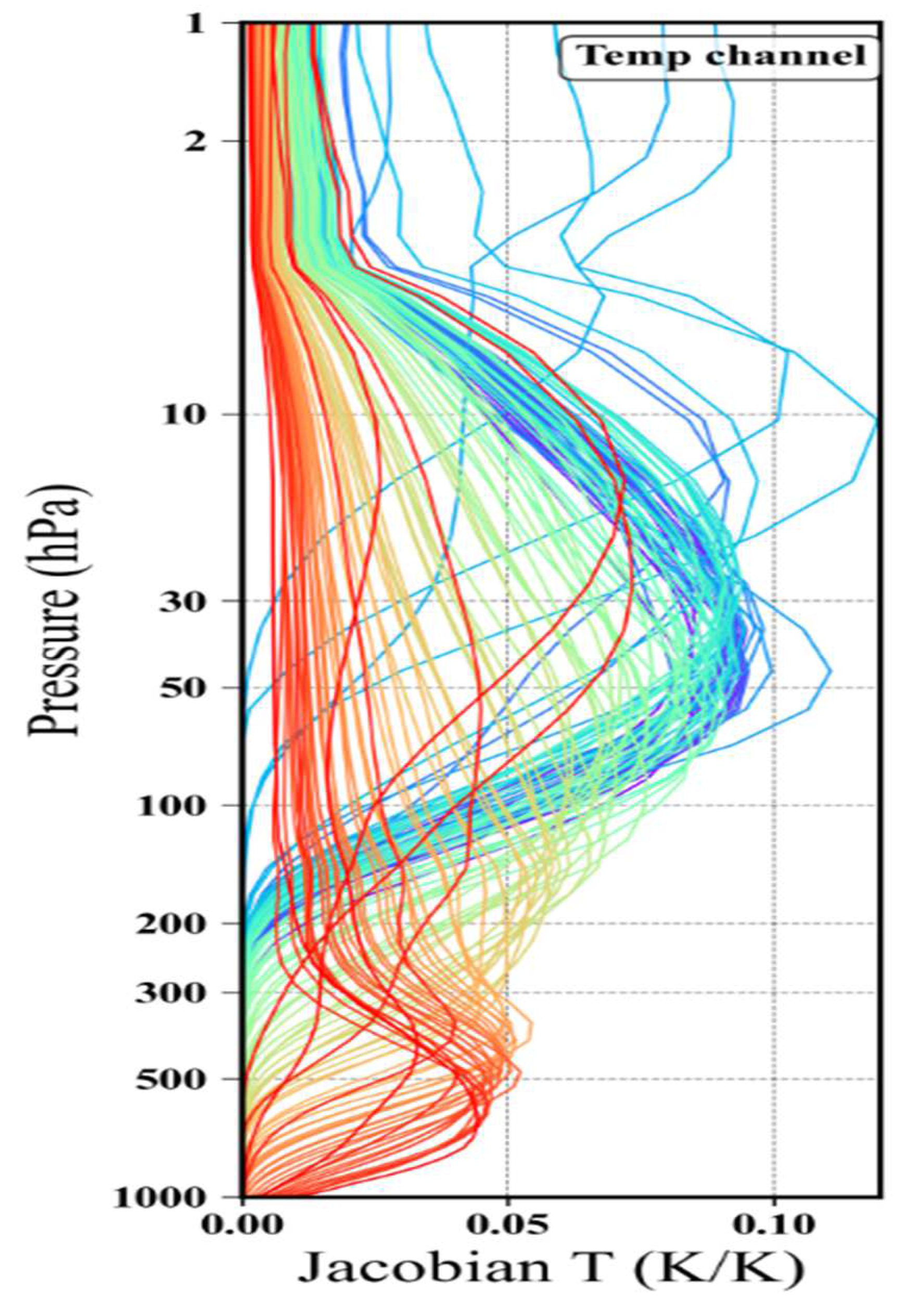
As listed in
Table 2, 56 CO
2 channels of FY-3E HIRAS are selected for assimilation by combining information entropy method and the weighting function peak [
44,
45]. The weighting function of the 56 channels was given in
Figure 1. Observation thinning was performed prior to 4DVAR by selecting the first pixel in 3 × 3 arrays of FOVs [
19] and sampling observations with a 200 km thinning radius to reduce the large satellite datasets.
Table 2.
Experiment schemes.
Table 2.
Experiment schemes.
| Experiments Scheme | Assimilation Data |
|---|
| CTRL | Same as Table 3 |
| FY3EHIRAS | CTRL + 56 IR Channel of FY-3E HIRAS (671.25 cm−1, 671.875 cm−1, 672.5 cm−1, 673.125 cm−1, 673.75 cm−1, 674.375 cm−1, 675 cm−1, 675.625 cm−1, 676.25 cm−1, 676.875 cm−1, 677.5 cm−1, 678.125 cm−1, 678.75 cm−1, 679.375 cm−1, 680 cm−1, 681.25 cm−1, 681.875 cm−1, 682.5 cm−1, 683.125 cm−1, 683.75 cm−1, 684.375 cm−1, 685 cm−1, 685.625 cm−1, 686.25 cm−1, 687.5 cm−1, 688.125 cm−1, 688.75 cm−1, 689.375 cm−1, 690 cm−1, 691.25 cm−1, 692.5 cm−1, 693.125 cm−1, 693.75 cm−1, 694.375 cm−1, 695 cm−1, 695.625 cm−1, 696.25 cm−1, 697.5 cm−1, 698.125 cm−1, 698.75 cm−1, 700 cm−1, 701.25 cm−1, 702.5 cm−1, 703.125 cm−1, 703.75 cm−1, 706.25 cm−1, 707.5 cm−1, 708.125 cm−1, 710 cm−1, 711.25 cm−1, 711.875 cm−1, 713.125 cm−1, 713.75 cm−1, 715 cm−1, 716.25 cm−1, 717.5 cm−1) |
Table 3.
CMA-GFS4.0 observation and variables in the CTRL experiments.
Table 3.
CMA-GFS4.0 observation and variables in the CTRL experiments.
| Platform | Instrument | Variables |
|---|
| Conventional observation | TEMP | Wind, temperature, relative humidity |
| SYNOP | Air pressure |
| SHIP | Air pressure |
| BUOY | wind |
| AIREP | Wind, Temperature |
| NOAA15 | AMSUA | Radiance of 7 MV bands |
| NOAA18 | AMSUA, AMSUB | Radiance of 10 MV bands |
| NOAA19 | AMSUA, AMSUB | Radiance of 11 MV bands |
| NOAA20 | CRIS | Radiance of 80 IR bands |
| NOAA20 | ATMS | Radiance of 12 MV bands |
| Suomi-NPP | ATMS | Radiance of 12 MV bands |
| FY-3C | MWHS | Radiance of 2 MV bands |
| FY-3D | MWTS-2, MWHS-2,
MWRI, HIRAS | Radiance of 6 MV bands,
Radiance of 56 IR bands |
| FY-3E | MWTS-2, MWHS-2, MWRI | Radiance of 12 MV bands |
| FY-4A | GIIRS, AGRI | Radiance of 60 LWIR bands, radiance of 50 LWIR bands, radiance of 2 WV bands |
| FY-2H | S-VISSR | Radiance of 1 WV bands |
| Himawaii-8 | AHI | Radiance of 3 WV bands |
| METOP-A | AMSUA, AMSUB, IASI | Radiance of 8 MV bands, radiance of 47 IR bands |
| METOP-B | AMSUA, AMSUB, IASI | Radiance of 12 MV bands, radiance of 47 IR bands |
| METOP-C | AMSUA, AMSUB, IASI | Radiance of 8 MV bands, radiance of 47 IR bands |
COSMIC,
Metop-A/B/C GRAS, GRACE-A,
TerraSAR-X,
FY-3D GNOS | GNSS RO | Refractivity |
| | GPS-PW | Atmospheric column water vapor content |
FY-2H, FY-2G
GOES-16, GOES-18,
MeteoSat-10, Himawai-9 | AMVs | Wind |
4. Assimilation Experiments and Impact of FY-3E HIRAS on Analysis and Forecast
4.1. Experiments Design
Two sets of experiments during the period from 18 February to 30 March 2023 have been carried out to test the impact of the FY3E HIRAS data on CMA-GFS. A preliminary spin-up run over a period of 10 days was conducted to obtain more statistically reliable predictor coefficients for a bias correction of HIRAS radiance data. These 10 days also allow the control and experiment to deviate and acclimate to the new data. The following analysis focuses on the results from 1 to 30 March 2023 with the data from the 10 days prior dismissed.
The experiment CTRL serves as the control, encompassing routine ground-based observations, radiosonde data, ship and aircraft reports, alongside conventional observations, microwave and infrared data from more than 20 meteorological satellites, GPS occultation data, and cloud-derived wind, etc. These types of data are assimilated into the model due to the assimilation capabilities already present in CMA-GFS 4.0.
Table 3 shows the list of assimilated data.
The FY3EHIRAS experiment evaluates the assimilation impact of 56 additional channels from FY-3E HIRAS beyond what is assimilated in CTRL (as shown in
Table 2).
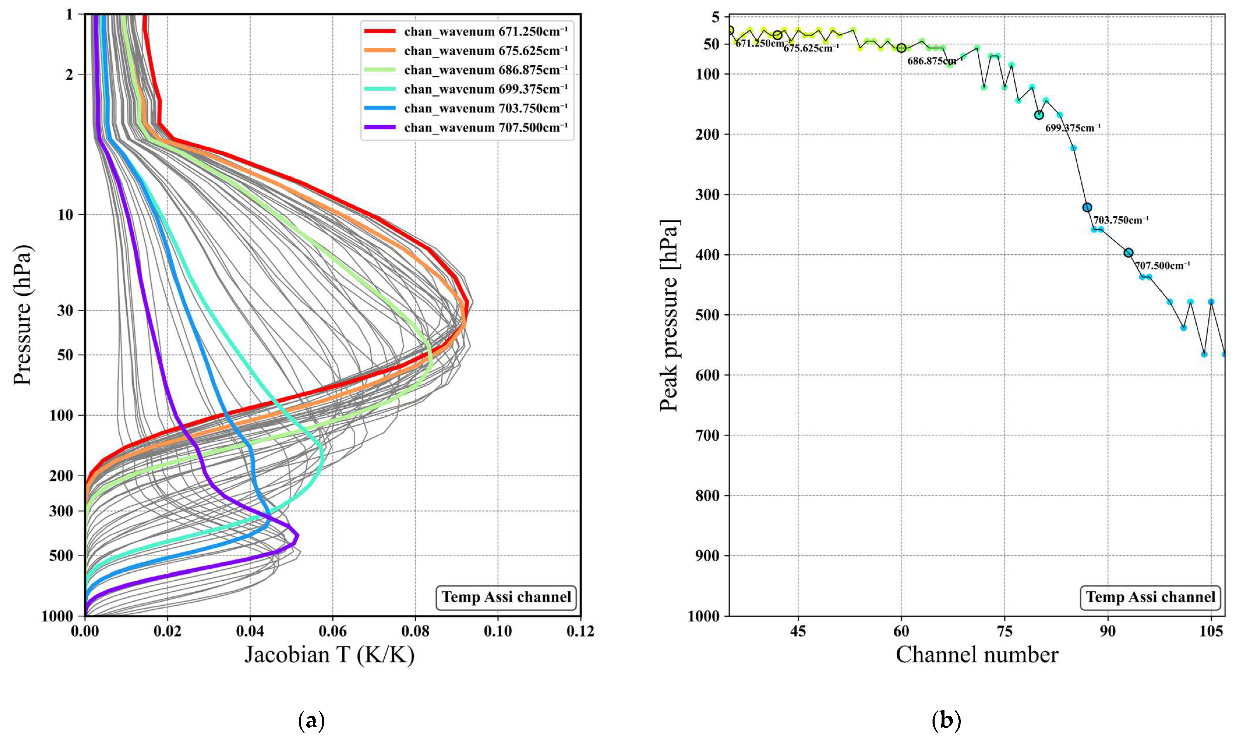
4.2. Analysis Fields Results
After bias correction, cloud detection, and quality control, the FY3E-HIRAS data were assimilated into CMA-GFS. Six channels (Channels 37, 44, 62, 82, 89, and 95) were selected and analyzed, which correspond to about 50 hpa, 70 hpa, 100 hpa, 200 hpa, 320 hpa, and 400 hpa based on the weighting function of each channel. The wave numbers of the six channels are 671.25 cm
−1, 675.625 cm
−1, 686.875 cm
−1, 699.375 cm
−1, 703.75 cm
−1, and 707.5 cm
−1 (as shown in
Figure 2).
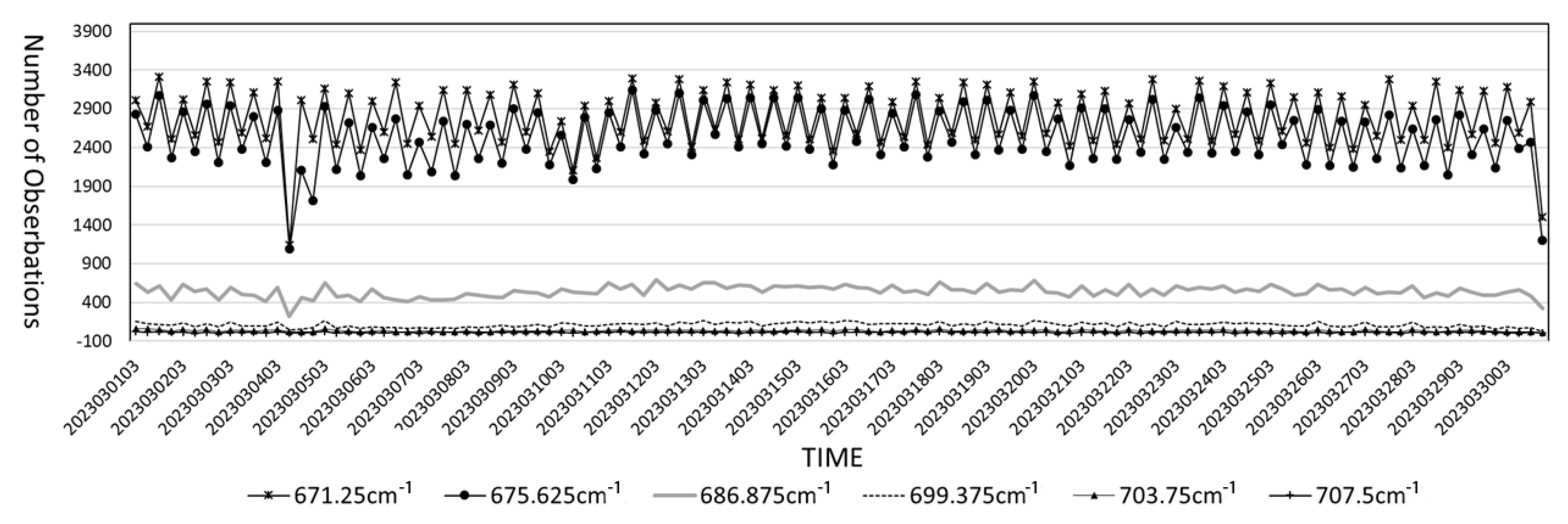
After bias correction, cloud detection, and quality control, the quantity of the FY3E HIRAS data assimilated into CMA-GFS from 1 March to 30 March 2023 is illustrated in
Figure 3. The results demonstrate that, due to the clear-sky channel cloud detection method (McNally and Watts), Channels 671.25 cm
−1 and 675.625 cm
−1 reside above the cloud tops, remaining unaffected by clouds. Consequently, after passing through additional quality controls, nearly 2400~3400 observations can be assimilated into the model every six hours. However, since Channels 686.875 cm
−1, 699.375 cm
−1, 703.75 cm
−1, and 707.5 cm
−1 are below the cloud top, following the cloud detection process, the data assimilated every six hours from these channels fluctuate between 100 and 800 observations. All channels maintain a consistent amount of daily assimilation.
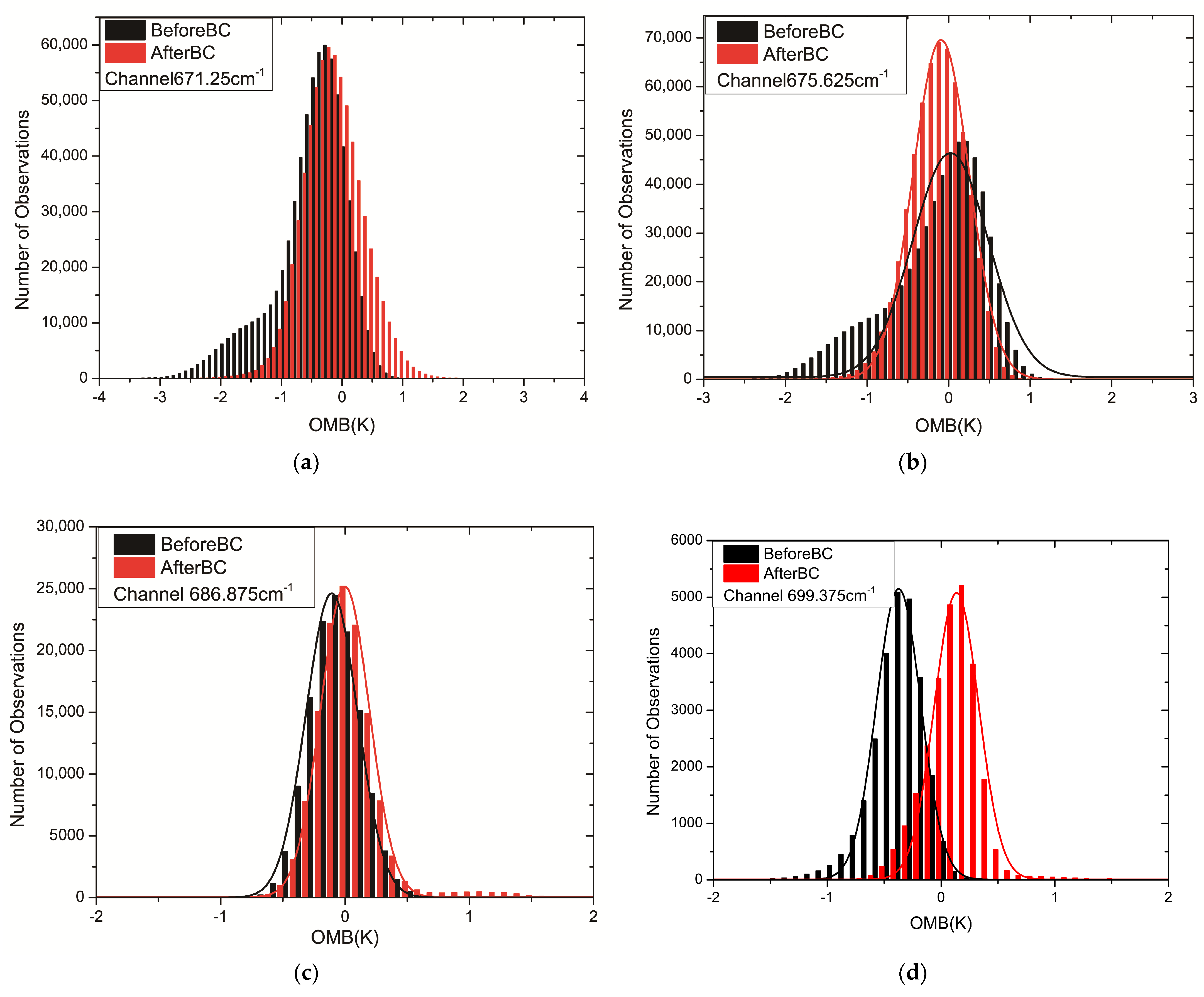
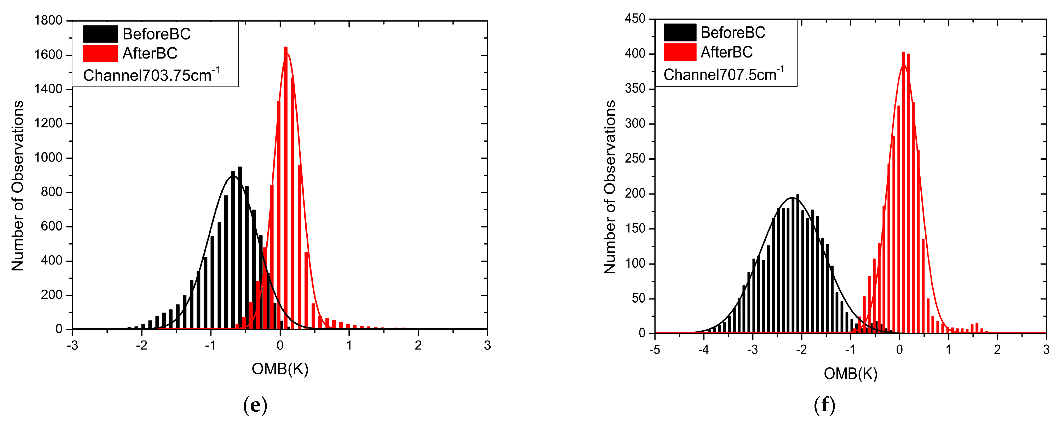
Figure 4 illustrates the probability density functions (PDFs) of the FY-3E HIRAS observation minus background (OMB) for Channels 671.25 cm
−1, 675.625 cm
−1, 686.875 cm
−1, 699.375 cm
−1, 703.75 cm
−1, and 707.5 cm
−1, both before and after bias correction. Initially, without bias correction, distinct channels exhibit varying degrees of deviation, with higher-level channels (Channels 675.625 cm
−1, 686.875 cm
−1, and 699.375 cm
−1) demonstrating deviations approximately within the −1 to 1 K range, while the channels 671.25 cm
−1 and 703.75 cm
−1 display deviations ranging from −2 to 2 K, and channel 707.5 cm
−1 exceeds 2 K. Following bias correction, the PDF distributions exhibit characteristics resembling a normal distribution, with the peaks of the OMB PDFs for several channels hovering around zero. These results signify that the OMB’s probability density function closely resembles a Gaussian distribution, meeting the requirement for variational assimilation.
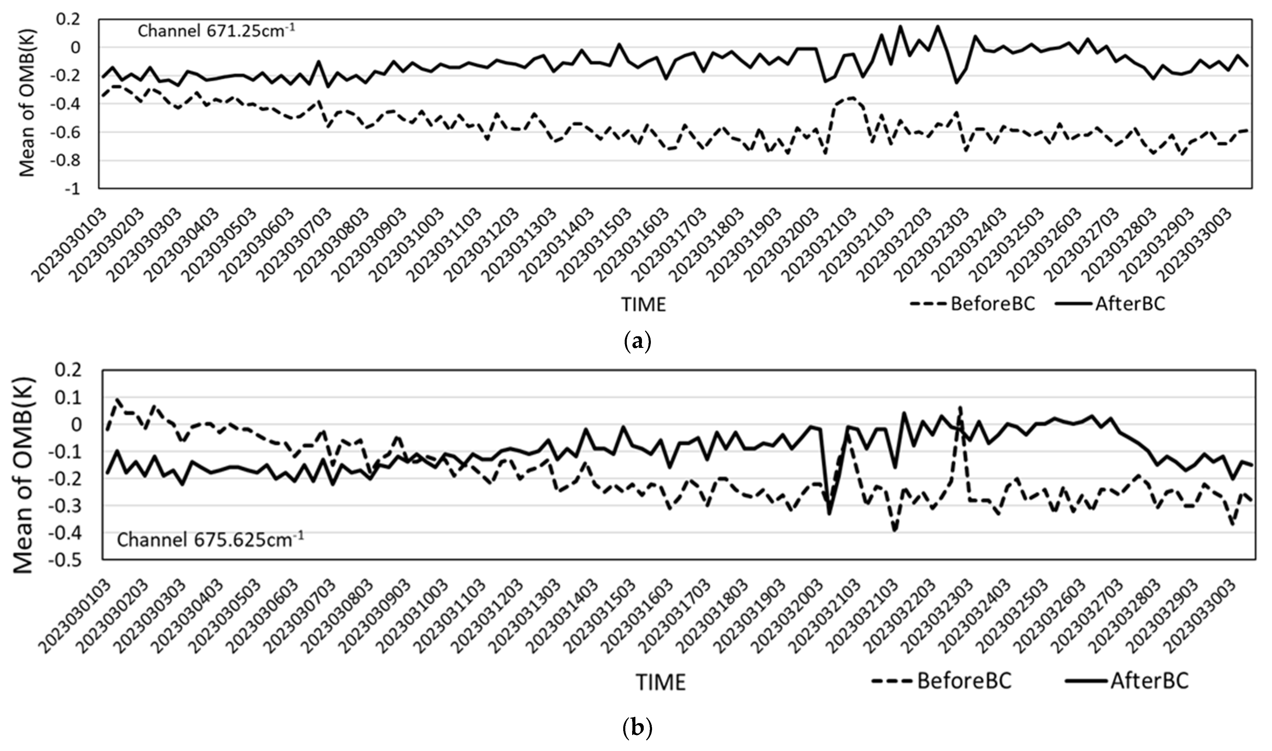
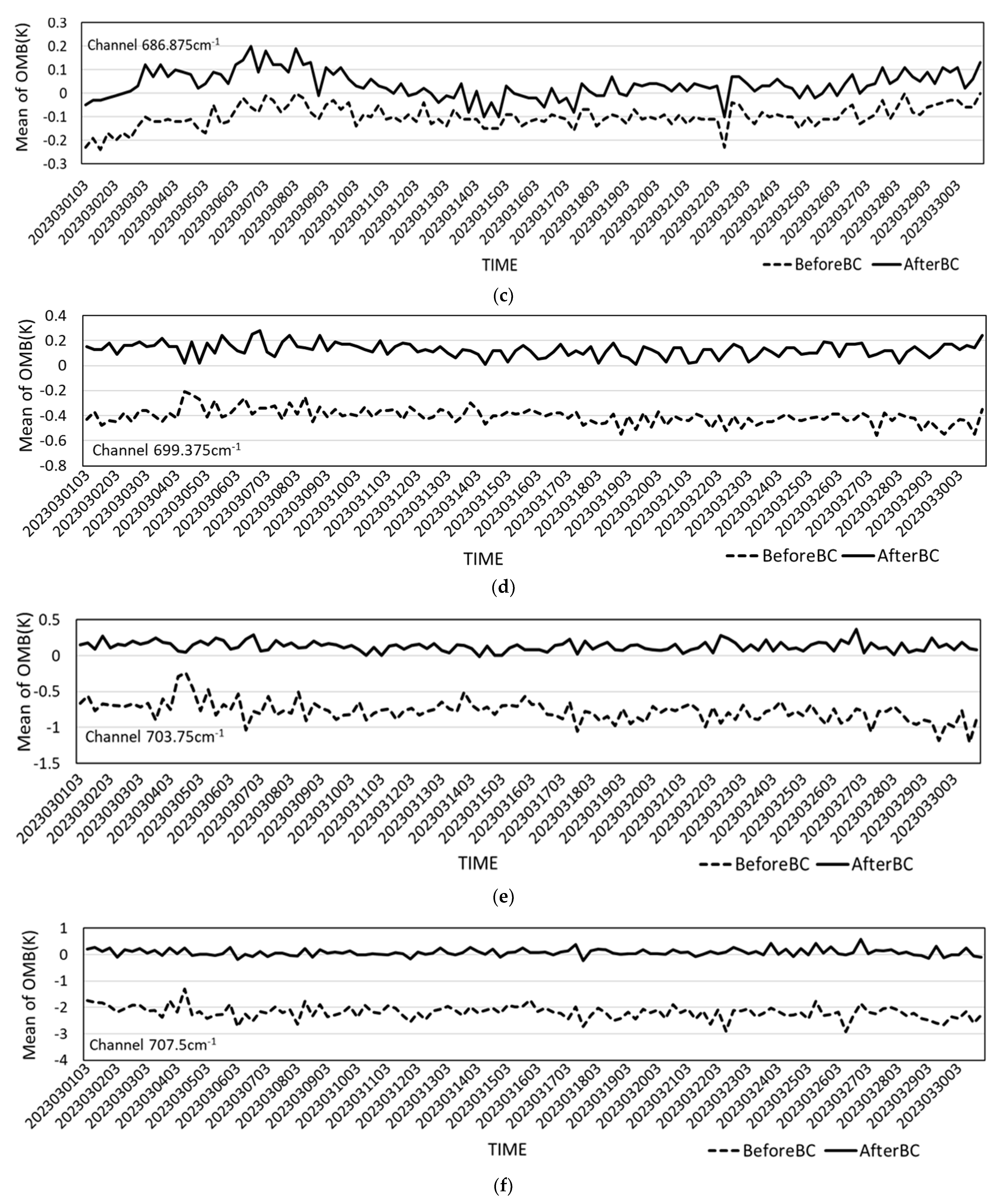
Figure 5 depicts the variation in the mean OMB of the FY-3E HIRAS data assimilated within each 6 h assimilation window for the six aforementioned channels before and after bias correction. Without bias correction, the OMB means of channels 671.25 cm
−1, 675.625 cm
−1, 686.875 cm
−1, and 699.375 cm
−1 are about −0.8~−0.2 K, −0.4~0.1 K, −0.25~0 K, and −0.5~−0.2 K, respectively. Channels 703.75 cm
−1 and 707.5 cm
−1 show higher deviations around −1.2~0.2 K and −2.5~−1.3 K, respectively. The OMBs of Channels 671.25 cm
−1 and 675.625 cm
−1 OMB display some instability, while the other channels remain relatively stable before bias correction. Following bias correction, notable reductions in OMB are observed across all six channels, with bias predominantly hovering around 0 K.
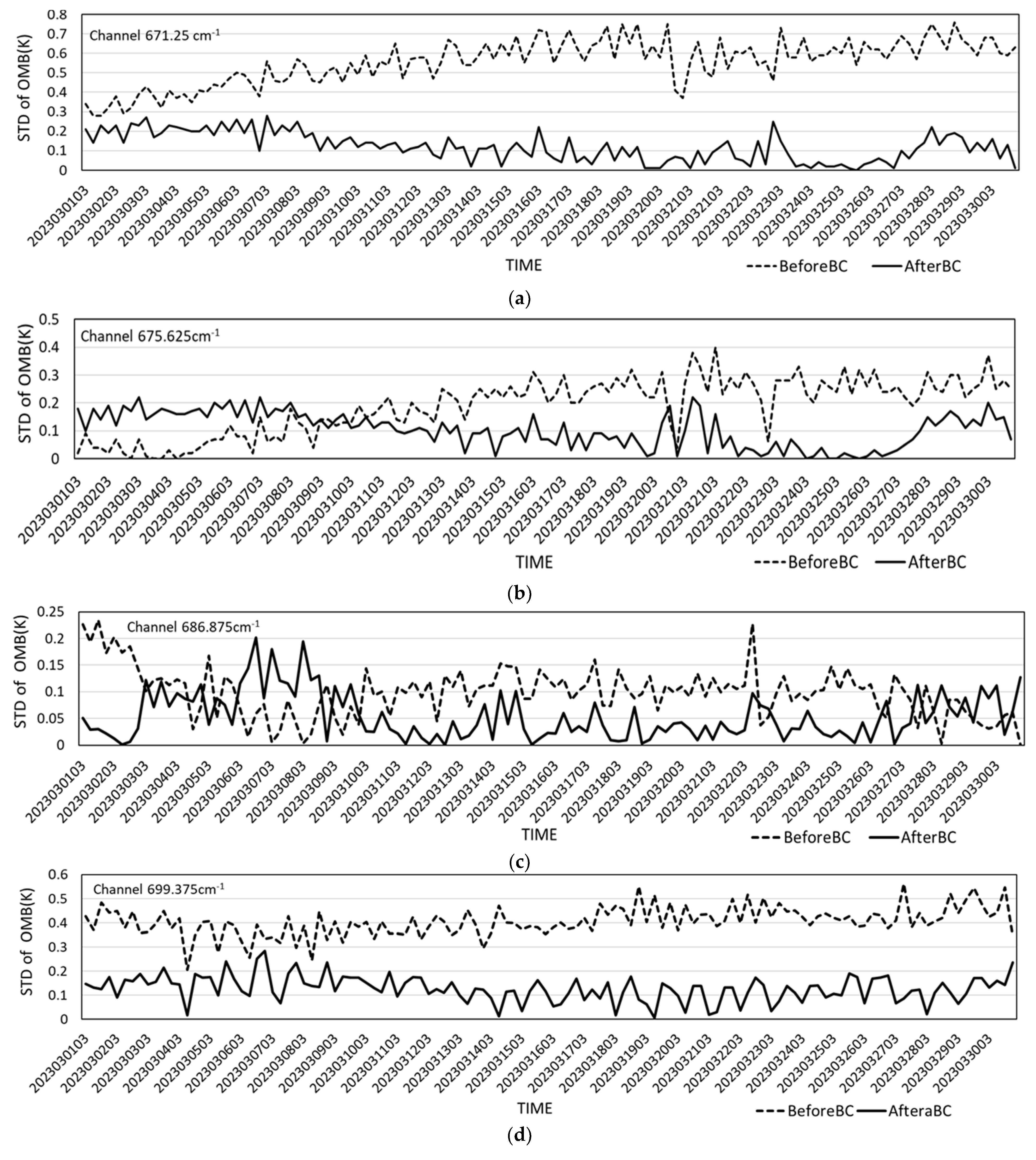
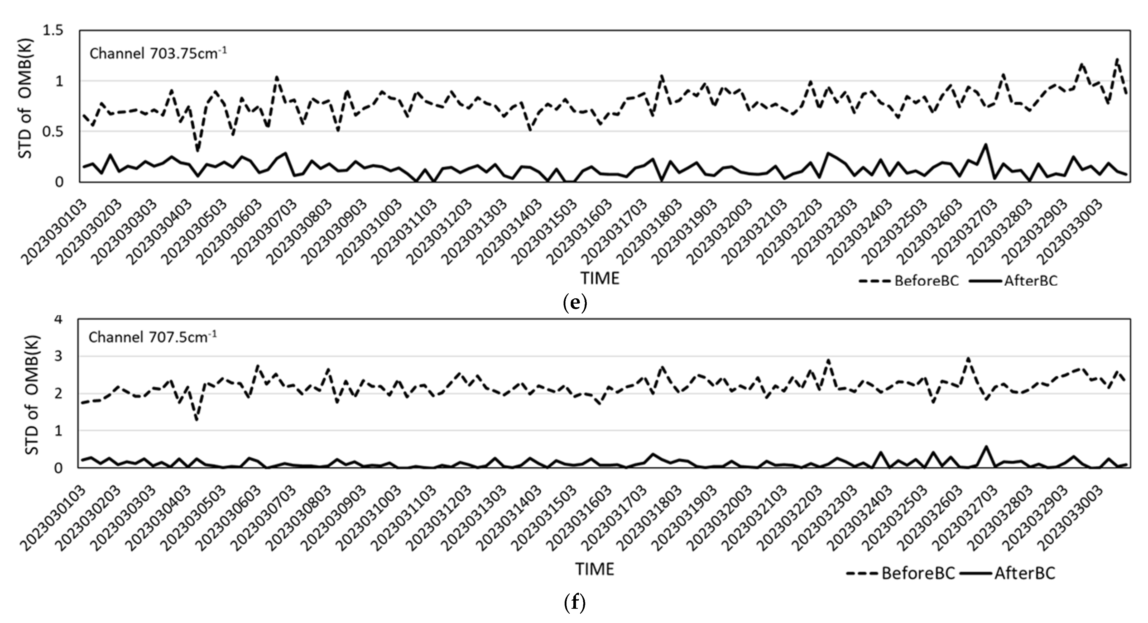
Figure 6 displays the temporal changes in the standard deviation (STDs) of the OMB for the FY-3E HIRAS data assimilated within each 6 h assimilation window for Channels 671.25 cm
−1, 675.625 cm
−1, 686.875 cm
−1, 699.375 cm
−1, 703.75 cm
−1, and 707.5 cm
−1, both before and after bias correction. Before bias correction, Channels 675.625 cm
−1, 686.875 cm
−1, and 699.375 cm
−1 exhibited STDs within the range of 0~0.5, Channel 671.25 cm
−1 displayed an STD between 0.28 and 0.8, while Channels 703.75 cm
−1 and 707.5 cm
−1 showed STDs larger than the other channels. The STDs display some fluctuation over an extended period before bias correction. After bias correction, the STDs for several channels approached zero and demonstrated more stability than that before bias correction during the experiment period. In summary, smaller STD values ensure the effective assimilation of the FY-3E HIRAS data into the CMA-GFS 4DVAR model.
4.3. Influence on the Analysis Fields with FY-3E HIRAS Data Assimilation
To assess the impact of the FY-3E HIRAS radiance data on the CMA-GFS analysis fields, ECMWF operational reanalysis data (ERA5) were utilized as an independent reference to evaluate the influence on key parameters of the model’s initial fields. The root mean square error (RMSE) relative to ERA5 was calculated separately for the FY3EHIRAS and CTRL experiments, and the RMSE reduction rate was plotted for the Southern Hemisphere, Northern Hemisphere, and the tropical region. RMSE serves as a measure to assess the deviation between two fields, indicating the extent of departure of the analysis field of two sets of experiments from that of the ERA5. Larger RMSE values imply a greater deviation of the CMA-GFS analysis field from the ERA5 field.
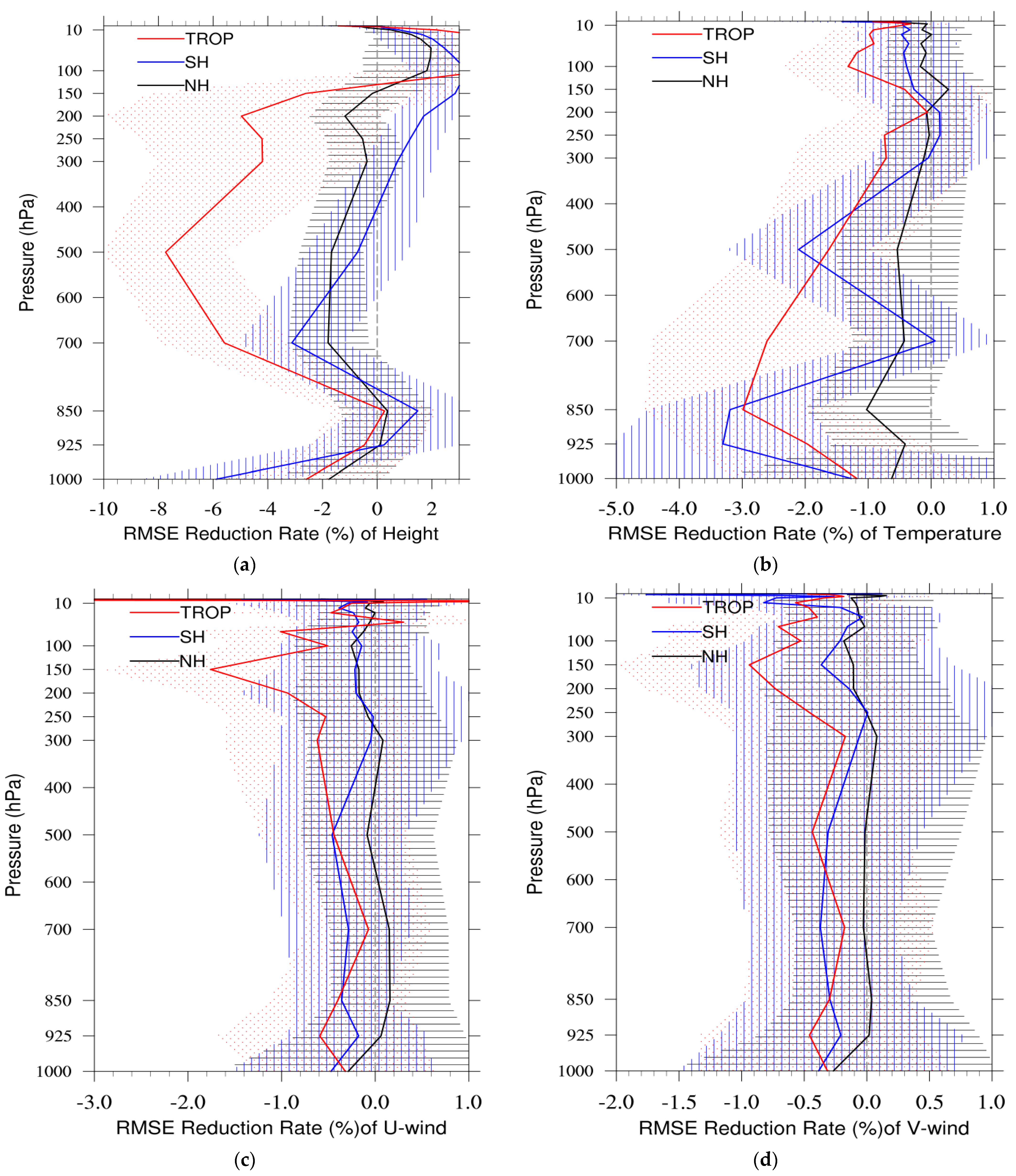
To further analyze the impact of the FY-3E HIRAS data assimilation across different levels of analysis fields, the reduction rate of RMSE in the FY3EHIRAS experiment relative to the CTRL experiment at each analysis time (t) is calculated using Formula (1):
where
is the analysis variable. Averaging the experimental cycle numbers yields the average reduction rate. From the formula, it can be inferred that a negative average reduction rate indicates an improvement in the analysis fields.
The reduction rate of RMSE for the temperature field (
Figure 7b) shows predominantly negative values overall, except for a slight increase observed in the Northern Hemisphere between 300 and 200 hPa and in the Southern Hemisphere between 200 and 150 hPa. Below 850 hPa, there is a notably significant reduction in RMSE in both the Southern Hemisphere and the tropics, with the maximum reaching 3%. A significant reduction region also appears in the Southern Hemisphere at 500 hPa, achieving a reduction rate of 2%. RMSE reductions are observed across other layers, notably in the tropics, followed by the Southern Hemisphere and then the Northern Hemisphere. Overall, assimilating FY-3E HIRAS CO
2 channels data results in an improvement in the temperature field.
The reduction rate of RMSE for the height field (
Figure 7a) indicates an increase at 850 hPa and above 150 hPa, while other layers exhibit a significant decrease. Notably, in the Southern Hemisphere and the tropics, there is a substantial reduction in RMSE for the height field between 850 hPa and 150 hPa, with a prominent decrease of 8% in the tropics at 500 hPa and 6% at 700 hPa. The Southern Hemisphere shows a reduction of 3% at 700 hPa, while the Northern Hemisphere’s reduction is slightly smaller compared to the other two regions, reaching around 2% at 700 hPa. At 200 hPa, there is a reduction of 5% with the tropical region and 2% with Northern Hemisphere. Overall, assimilating FY-3E HIRAS data demonstrates a predominantly positive effect on the analysis of the height field relative to ERA5.
The RMSE for the U-wind and V-wind fields in the Southern Hemisphere and the tropics demonstrates a reduction across all atmospheric layers. The reduction rate for the U-wind field (
Figure 7c) in the Southern Hemisphere reaches approximately 0.4% between 1000 hPa and 500 hPa. While the Northern Hemisphere shows smaller reductions, with a negative value between 600 hPa and 400 hPa and above 250 hPa, and slight increments in other layers, around 0.1% increment between 925 hPa and 700 hPa. Significantly, the reduction rate of RMSE after the assimilation of FY-3E HIRAS in the U-wind field for the tropics is most prominent, with about 0.2% between 850 hPa and 500 hPa and exceeding 0.5% in other layers, even reaching 2% in higher layers. The RMSE reduction rate for the V-wind field (
Figure 7d) follows a similar vertical distribution trend as the U-wind field, but slightly better than the U-wind field in the Northern Hemisphere between 925 hPa and 700 hPa. Overall, the assimilation of FY3E HIRAS data has reduced the analysis errors in both the U and V wind fields.
Based on the comprehensive analysis, assimilating FY-3E HIRAS data has led to some extent of improvement in the initial fields of temperature, wind, and height within CMA-GFS comparing with ERA5 data.
5. Impact on CMA-GFS Forecasts with FY-3E HIRAS Data Assimilation
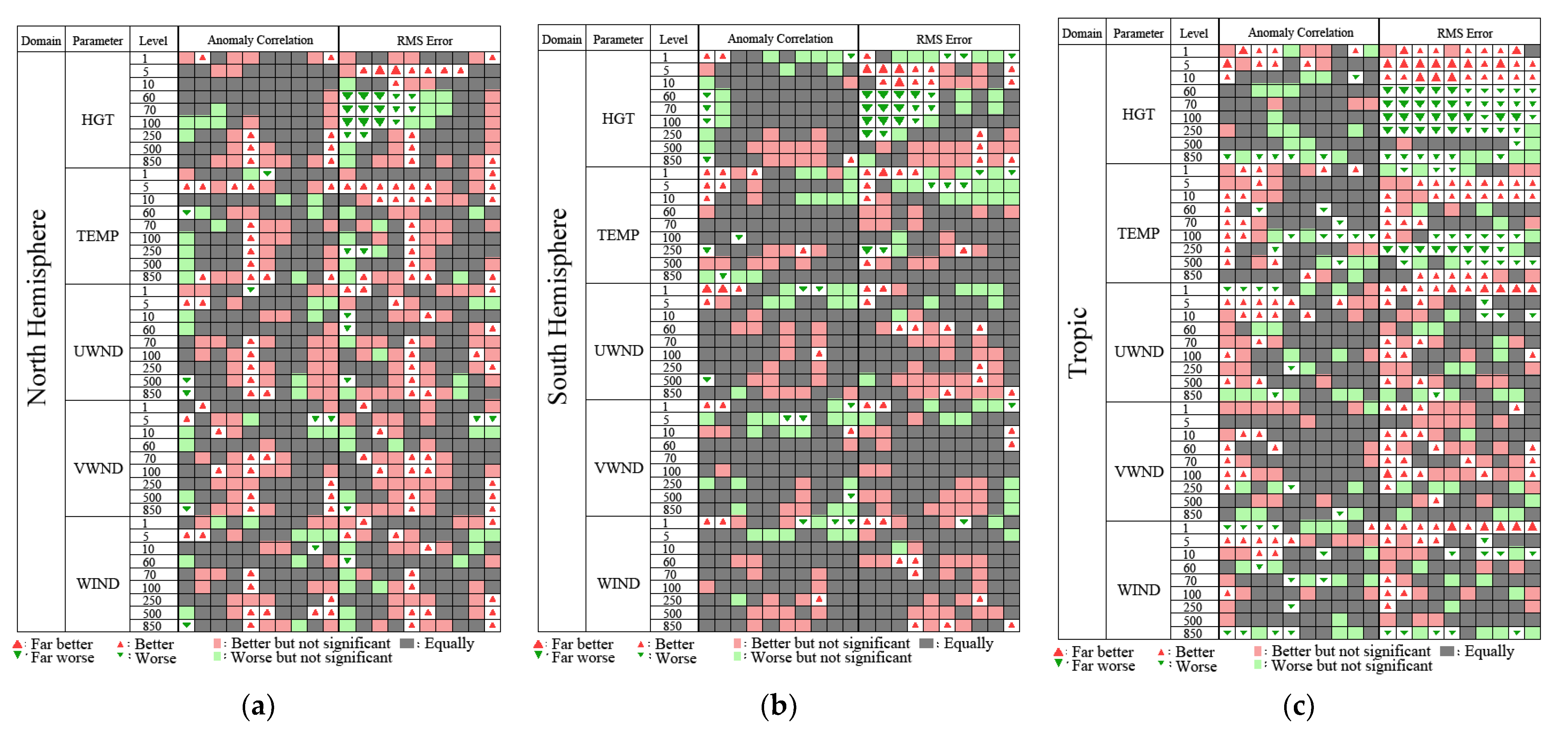
To assess the influence of FY-3E HIRAS data on CMA-GFS forecasts, 240 h forecasts were conducted for FY3EHIRAS and CTRL experiments. These forecast experiments were performed in 12 h cycling runs for a period of one month, from 1 March to 30 March 2023. During this period, forecasts up to a range of 240 h were started at 0000 and 1200 UTC. Initially, the CMA-GFS standard forecast scorecard is employed to highlight the changes in the forecasts for key atmospheric variables between FY3EHIRAS and CTRL experiments at lead times from 12 to 240 h, and is validated against ERA5 data for key atmospheric variables. The scorecard includes seven categories, namely far better, better, better but not significant, equally, far worse, worse, and worse but not significant. This scorecard includes subjective assessments of the selected parameters compared against corresponding verifications for sensitivity tests and control modeling. It functions as a rapid tool for users to comprehend the fundamental model performance, based on the significance tests of statistical variables. For detailed definitions, refer to [
46].
The forecast impact scorecard for FY-3E HIRAS is shown in
Figure 8, where the red color indicates improvement, green color means getting worse, and gray color represents a comparable effect. The size of the triangles indicates the significance of the impact. The scorecard value of worse can be observed with RMS for the height field forecast in the first 5 days for the Northern Hemispheres, Southern Hemispheres, and Tropical region. Temperature and wind fields show a slight improvement or neutral effect overall. The temperature field exhibits a significant improvement in the upper level.
For global forecasts, ACC (anomaly correlation coefficient) and RMSE are commonly employed to measure the forecasting skills of global models. ACC assesses the linear correlation between the forecast and analysis fields, determining the similarity between two spatial variable fields [
47].
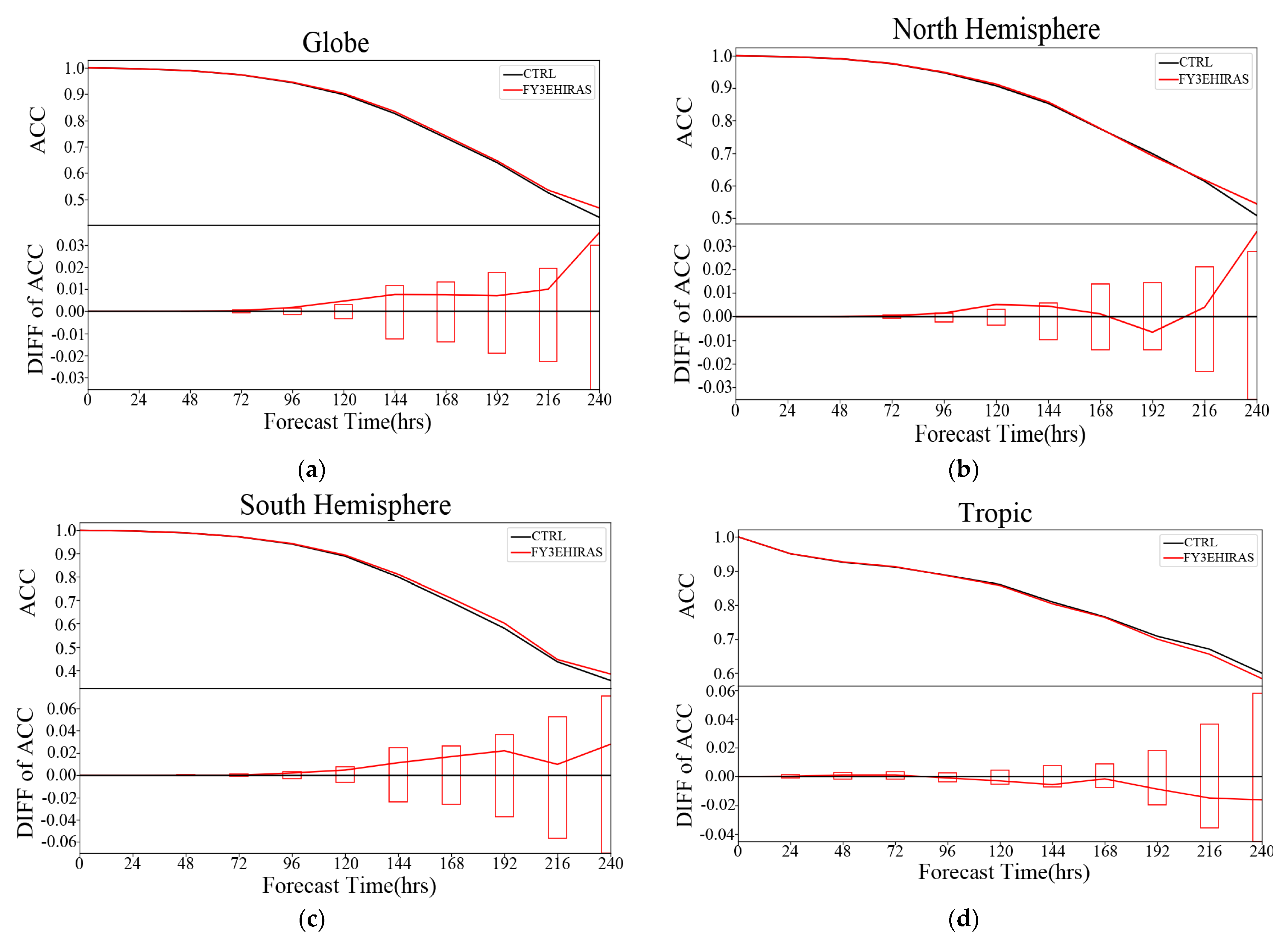
A higher ACC indicates greater similarity between the forecast and analysis fields, signifying the better forecasting performance of the model. According to the World Meteorological Organization (WMO) standards, a forecast for the 500 hPa height field is considered effective when its ACC exceeds 0.6.
Figure 9 presents the distribution of ACC for the 500 hPa geopotential height field for the globe (
Figure 9a), Northern Hemisphere (
Figure 9b), Southern Hemisphere (
Figure 9c), and Tropical Region (
Figure 9d). It is noticeable that for, the global forecasts in both experiments, ACC starts to improve from 72 h onwards with FY-3E HIRAS data assimilation. In the Northern Hemisphere, ACC surpasses CTRL from 72 h, decreases by 192 h, and improves again after 216 h. Conversely, in the Southern Hemisphere, ACC notably exceeds CTRL after 72 h. These results align with the expectation that the Southern Hemisphere would exhibit more pronounced effects compared to the Northern Hemisphere because the Southern Hemisphere has limited conventional observation data due to its oceanic dominance, but observational data in the Northern Hemisphere are more abundant. For the forecast of the tropical region, as shown in
Figure 9d, the ACC of 500 hpa geopotential height was basically the same as the CTRL experiment in the first 96 h, but decreased after 96 h. Therefore, after assimilating the FY-3E HIRAS data, there was no positive effect on the forecast for the tropical region.
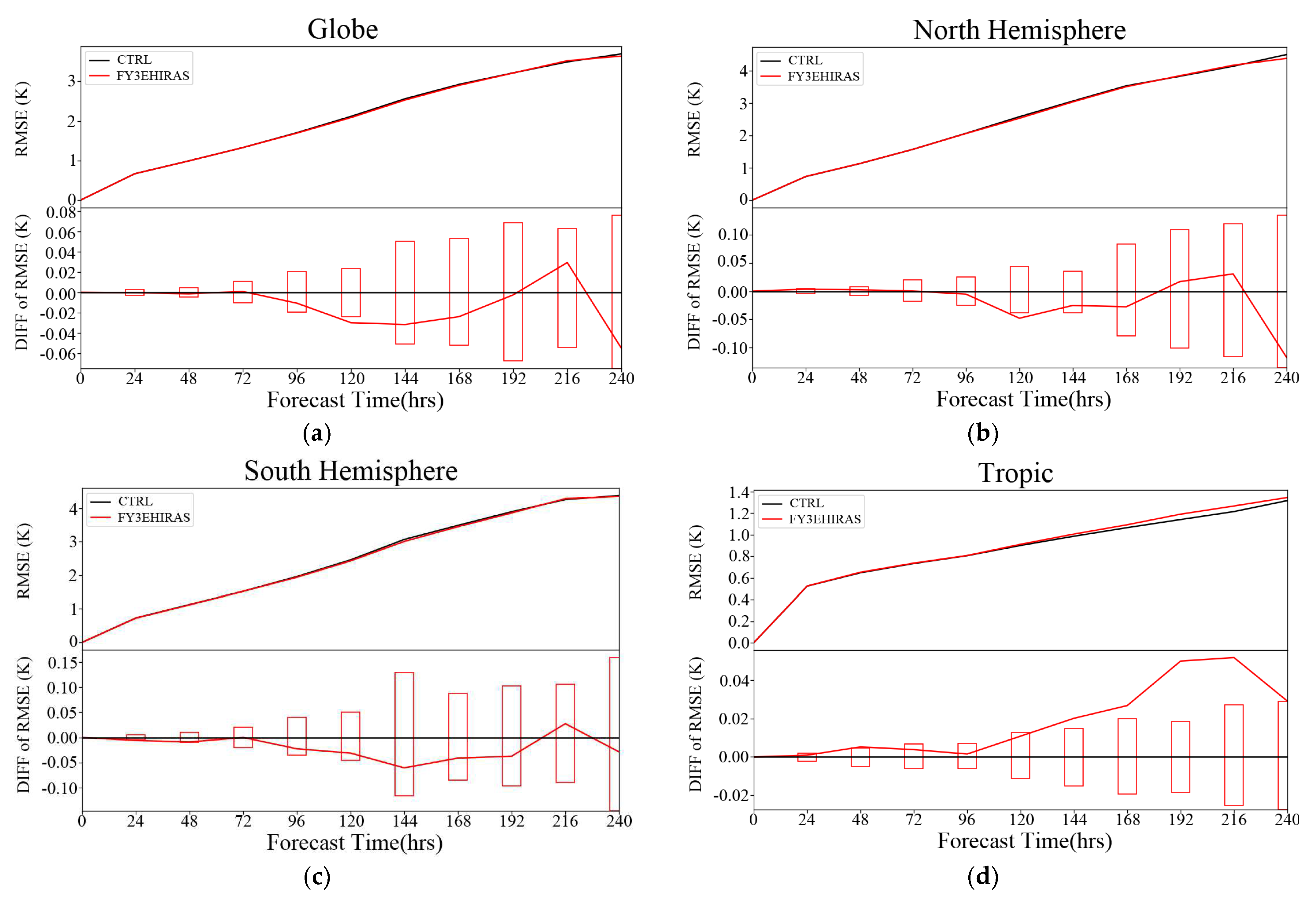
Figure 10 illustrates the variations in RMSE for the forecasted 500 hPa temperature field across the globe (
Figure 10a), Northern Hemisphere (
Figure 10b), Southern Hemisphere (
Figure 10c), and Tropical Region (
Figure 10d). In upper-BOX, the black and red lines represent the RMSE of the T + 12 to T + 240 h 500 hPa temperature forecast relative to ECMWF forecast for CTRL and FY3EHIRAS, respectively. In bottom-BOX, the red line represents the difference in RMSE between the FY3EHIRAS and CTRL forecasts, with negative values indicating a reduction in RMSE.
It is evident that, within the initial 72 h, the temperature forecasts in both experimental sets are fairly comparable. However, following the assimilation of FY-3E HIRAS data, the 72–192 h temperature forecasts for the entire globe exhibit a closer alignment with ECMWF’s forecast. In the Northern Hemisphere, the 96–168 h temperature forecasts align more closely with ECMWF, while in the Southern Hemisphere, the 72–192 h temperature forecasts show improved alignment with ECMWF. Similar analyses for other layers (figures omitted) reveal consistent outcomes in the upper layers, with very little changes in the lower layers. However, for the tropical region, adding FY-3E HIRAS showed a negative effect on the forecasts.
6. Summary and Discussion
This study investigates the impact of assimilating FY-3E HIRAS radiance data on the analysis and forecast of the global NWP model CMA-GFS. A data assimilation algorithm, incorporating data quality control, bias correction, cloud detection, data thinning schemes, and apodization for FY-3E HIRAS, is designed based on the CMA-GFS 4DVAR assimilation system. The DA impact of FY-3E HIRAS data is examined by comparing the experiment of additionally assimilating FY3EHIRAS with the CTRL experiment. With quality control, bias correction, and cloud detection, the OMB‘s PDFs of the FY-3E HIRAS data assimilated into the model exhibit characteristics of a Gaussian distribution, meeting the requirements of variational data assimilation.
A data assimilation framework for FY-3E HIRAS radiance is implemented on the CMA-GFS 4DVar platform. A month-long batch experiment is conducted to assess the impact of assimilating FY-3E HIRAS 56 CO2 channels on analysis and forecast in CMA-GFS 4DVar.
The assimilation of FY-3E HIRAS data significantly reduces the error in the CMA-GFS temperature analysis field compared to the CTRL experiment in the Southern and Northern Hemispheres. In comparison to ERA5 reanalysis data, the RMSE reduction rate for temperature field generally exhibits negative values, except for slight increases between 300 and 200 hPa in the Northern Hemisphere and 200 and 150 hPa in the Southern Hemisphere after assimilating FY-3E HIRAS data. Notably, there is a substantial decrease in RMSE below 850 hPa, with the most significant reductions observed in the Southern Hemisphere and the tropical region, reaching up to 3% and 2% at 850 hPa and 500 hPa, respectively. This suggests a better temperature analysis field compared to the CTRL experiment. Additionally, improvements in the height and wind fields are observed to some extent. Regarding forecasting, the assimilation of FY-3E HIRAS data results in a neutral or slight improvement in the forecast skills in the Southern Hemisphere, Northern Hemisphere, and the tropical region.
CMA-GFS currently assimilates multiple data sources, including data from more than 20 satellites, conventional observations, and cloud derived wind, occultation data and other data. Although the inclusion of FY-3E HIRAS data demonstrates some improvements in the forecast capabilities with the global model, due to the multitude of existing data sources, the impact is not substantially significant. Nevertheless, there is considerable potential to enhance the assimilation effect of FY-3E HIRAS data, particularly through further refinement of the cloud detection algorithm, using more channels, and optimizing sparse radius, etc.
Our results show a more prominent improvement in the analysis field in SH and PBL which indicates that adding the FY-3E dawn–dusk data does help the data-sparse regions more. This further demonstrates the application value of the dawn–dusk orbit satellite data in the NWP model. However, further exploration is needed to evaluate why there is a significant impact with the analysis field on the PBL in the future.
Future research will concentrate on enhancing the design of the optimal data thinning scheme and advancing cloud detection algorithms to address issues related to data inefficiency and insufficient information extraction in the current schemes. This will ultimately elevate the efficacy of FY-3E HIRAS assimilation. In addition, this study has not yet involved the assimilation of water vapor channels. Future research will also conduct evaluation and prediction impact studies on FY-3E HIRAS water vapor channels data to deeply and fully take advantages of dawn–dusk orbit satellite.


