
Multiobjective Evolutionary Superpixel Segmentation for PolSAR Image Classification
by
 , , ,
, , ,
Boce Chu
1,2,
Mengxuan Zhang
3,*,
Kun Ma
3,
Long Liu
4,
Junwei Wan
5,
Jinyong Chen
2,
Jie Chen
1 and
Hongcheng Zeng
1 1
School of Electronics and Information Engineering, Beihang University, Beijing 100191, China
2
54th Research Institute of China Electronics Technology Group Corporation, Shijiazhuang 050081, China
3
Key Laboratory of Intelligent Perception and Image Understanding of Ministry of Education, School of Artificial Intelligence, Xidian University, Xi’an 710071, China
4
School of Engineering, Xidian University, Xi’an 710071, China
5
Beijing Institute of Remote Sensing Information, Beijing 100192, China
*
Author to whom correspondence should be addressed.
Remote Sens. 2024, 16(5), 854; https://doi.org/10.3390/rs16050854
Submission received: 9 January 2024
/
Revised: 24 February 2024
/
Accepted: 27 February 2024
/
Published: 29 February 2024
(This article belongs to the Special Issue Object Detection and Information Extraction Based on Remote Sensing Imagery)
Abstract
:Superpixel segmentation has been widely used in the field of computer vision. The generations of PolSAR superpixels have also been widely studied for their feasibility and high efficiency. The initial numbers of PolSAR superpixels are usually designed manually by experience, which has a significant impact on the final performance of superpixel segmentation and the subsequent interpretation tasks. Additionally, the effective information of PolSAR superpixels is not fully analyzed and utilized in the generation process. Regarding these issues, a multiobjective evolutionary superpixel segmentation for PolSAR image classification is proposed in this study. It contains two layers, an automatic optimization layer and a fine segmentation layer. Fully considering the similarity information within the superpixels and the difference information among the superpixels simultaneously, the automatic optimization layer can determine the suitable number of superpixels automatically by the multiobjective optimization for PolSAR superpixel segmentation. Considering the difficulty of the search for accurate boundaries of complex ground objects in PolSAR images, the fine segmentation layer can further improve the qualities of superpixels by fully using the boundary information of good-quality superpixels in the evolution process for generating PolSAR superpixels. The experiments on different PolSAR image datasets validate that the proposed approach can automatically generate high-quality superpixels without any prior information.
1. Introduction
Synthetic Aperture Radar (SAR) is not sensitive to atmospheric and lighting conditions [1]. Polarimetric SAR (PolSAR) can enhance the performance of SAR in acquiring targets and more specific information on targets, which plays an important role in national defense, military reconnaissance, agricultural monitoring, and many other fields [2,3]. The traditional pixel-based PolSAR image interpretation results may bring a huge amount of computation and contain many misclassification regions resulting from speckle noise. Addressing the above issues, superpixel generation becomes an important step in PolSAR interpretation [4,5]. A superpixel is a set of continuous small regions composed of adjacent pixels with similar characteristics in the image, which can retain the spatial feature information of the original image. The image processing based on superpixels can improve efficiency greatly and reduce the influence of speckle noise in PolSAR images [6,7,8].
The superpixel generation approaches can be divided into two categories, cluster-based methods and graph-based methods. The cluster-based methods group pixels into multiple clusters, and each cluster is a superpixel block. The current mainstream cluster-based methods mainly include simple linear iterative clustering (SLIC) [9], energy-driven sampling (SEEDS) [10], Turbopixel (TP) [11], linear spectral clustering (LSC) [12], mean shift (MS) [13], quick shift (QS) [14], and depth-adaptive superpixel (DAS) [15]. SLIC is a linear iterative clustering method that generates superpixels by assigning pixels to the most relevant seeds within a fixed distance range. SLIC needs to set the number of superpixels in advance and has linear time complexity, where linear time complexity refers to the linear relationship between the execution time occupied by the algorithm and the input image size. SEEDS utilizes the guidance of energy function to find the optimal path on the image. Since only the pixels near the edge of the superpixel are considered, the calculation efficiency is high. TP is a more commonly used morphological method, which uses a geometric flow method to construct a set of regularly distributed seeds. The generated superpixels have good uniformity and compactness while the edge fitting is poor. Although TP has linear complexity, it is much slower than SLIC. LSC can improve the superpixel segmentation performance by using the kernel function to achieve normalized cutting, which retains the global properties of the image. MS is a non-parametric clustering and density estimation method that finds the cluster centers of the data by finding the regions with the highest probability densities in the data distribution. It does not need to set the number of superpixels in advance. However, it is still sensitive to the initialization and the noise, and the computational complexity is high. QS simply moves each pixel to the nearest pixel where the probability density increases. It can generate relatively good boundary compliance for superpixels without the need to specify the number of superpixels in advance. With the depth information of the image, DAS can generate superpixels in real-time by calculating the density of the superpixel cluster and updating the cluster center using a multi-scale method. Graph-based methods include normalized Cut (N-cut) [16], Graph-Based Segmentation (GS) [17], Pseudo-Boolean (PB) [18], and Lazy Random Walk (LRW) [19]. N-cut minimizes the global segmentation error by normalizing the eigenvector of the Laplacian graph matrix, but its operation efficiency is not good enough. GS is an efficient graph-based segmentation algorithm that requires cohesive clustering and minimum spanning tree construction. The superpixels generated by GS have good edge fitting, but the shapes and sizes are irregular. PB transforms the superpixel segmentation into the label assignment problem, which is the binary labeling problem of the Markov random field. The number of superpixels does not affect the speed of PB, which breaks the bottleneck of the traditional algorithms. LRW is derived from the Random Walk algorithm (RW). After initialization, LRW moves seeds continuously through the guidance of energy function to achieve seed thinning.
Although the traditional superpixel generation approaches can achieve excellent performance on optical images, it is not feasible to apply these methods to PolSAR images directly to achieve enough segmentation performance. They do not consider the polarization information in PolSAR images at all. The traditional distance measurements are also not suitable for PolSAR images. Due to the different properties of ground targets, the search for the accurate boundaries of the superpixels becomes more complex and more difficult. Addressing the above issues, many improved superpixel segmentation techniques have been proposed in recent years. Qin et al. [20] improved the initialization and post-processing steps of SLIC to overcome the influence of speckle noise. Ersahin et al. [21] applied a spectral graph partitioning algorithm for PolSAR image superpixel segmentation and classification, which improved the performance of automated analysis through spatial proximity and graph segmentation. Xiang et al. [22] introduced polarization uniformity measurement from adaptive polarization and spatial information to control superpixels’ shapes and compactness. However, these approaches need to determine the number of superpixels manually in advance, which requires the designer’s rich prior knowledge. The number of superpixels has a significant impact on the final segmentation performance and the subsequent tasks. In addition, the objectives of traditional superpixel segmentation algorithms are defined as the weighted sum of different indexes to ensure the superpixel quality. These weights have a significant impact on the final segmentation performance, and are usually set as constants manually in advance. Obviously, it is not easy to determine the universal weights for all situations. Furthermore, most of the existing superpixel segmentation algorithms generate superpixels with uneven distribution and do not make full use of excellent superpixel information in the generation process. To deal with the above issues, this study proposes a multiobjective evolutionary superpixel segmentation (MOES) for PolSAR image classification. The superpixel generation for PolSAR images is defined as a multiobjective optimization without any weights set before, where the similarity information within the superpixels and the different information among the superpixels can be fully considered. The boundary information of excellent superpixels is introduced into the evolutionary operator to generate new superpixels with more accurate boundaries of complex ground targets in PolSAR images. With the optimal solutions obtained by multiobjective optimization for superpixel segmentation, the most suitable number of superpixels can be determined automatically, and high-quality superpixel segmentation can be achieved. MOES consists of two layers, an automatic optimization layer and a fine segmentation layer. The main contributions can be summarized as follows:
- The superpixel generation for PolSAR images is defined as a multiobjective optimization problem. the automatic optimization layer can optimize the similarity within the superpixels and the difference among the superpixels simultaneously. The suitable number of superpixels can be determined for the observed PolSAR image automatically.
- The fine segmentation layer can further improve the segmentation performance by fully using boundary information, where the boundary information of the good-quality superpixels is incorporated into the specific evolutionary operator to generate better superpixel segmentation results. It is helpful to search for the accurate boundaries of complex ground targets.
The rest of this study is organized as follows. The related works of PolSAR superpixel segmentation and multiobjective evolutionary algorithms are introduced first. Then, MOES is described in detail. In Section 4, the studies on MOES and the comparison experiments are analyzed. The conclusion and future work are provided last.
2. Related Works
2.1. Superpixel Segmentation for PolSAR Images
In recent years, a variety of superpixel segmentation techniques for PolSAR images have been proposed by introducing scattering information to ensure segmentation performance. The existing PolSAR superpixel segmentation methods can be divided into five categories: the density-based method [13], the graph-based method [16], the contour evolution method [11], the energy optimization method [23], and the cluster-based method [9]. For the density-based method, Lang et al. [24] proposed a generalized mean shift algorithm for PolSAR images. Through adaptive bandwidth and advanced processing strategies, the segmentation performance could be improved effectively. It is difficult for density-based algorithms to control the number of superpixels. As one of the graph-based approaches, Liu et al. [25] modified the N-cut algorithm by combining modified Wishart distance and edge graphs. Wang et al. [26] realized effective segmentation of homogenous and heterogeneous regions in PolSAR images by integrating different distance measures and introducing an entropy rate method. The graph-based methods are relatively complex and have high computational requirements. For the contour evolution method, Liu et al. [27] used a TP algorithm to segment PolSAR images into several superpixels and residual pixels for final classification. For the energy optimization method, Yang et al. [23] proposed a novel layered energy-driven PolSAR image segmentation method that used the histogram intersection of the coherence matrix and Wishart energy to generate coarse and fine-level superpixels, respectively. The computation of the energy optimization method is relatively high. Compared with other approaches, the cluster-based methods can obtain dense regions with controllable numbers and regular shapes. Most of the cluster-based methods utilize the principles of clustering algorithms and distance measurements based on both polarization and spatial information. Qin et al. [20] proposed a local iterative clustering superpixel generation algorithm that used Wishart distance to calculate the similarity between pixel points and then used the clustering method to generate superpixels. Hou et al. [28] proposed a decomposition feature iterative clustering method that used the decomposition of pixel features and spatial positions to cluster. It introduced a new pixel similarity and reduced the influence of speckle noise. Li et al. [29] proposed a new cross-iterative strategy for PolSAR superpixel segmentation that combined an improved Wishart distance and geodesic distance to generate stable superpixels with a high boundary recall rate (BR). Guo et al. [30] proposed an adaptive fuzzy super-pixel segmentation method that introduced the correlation of polarization scattering information into pixels and adjusted the proportion of undetermined pixels adaptively. Although these superpixel segmentation techniques can achieve good performance for PolSAR images, most of them need to determine the number of superpixels manually in advance. The number of superpixels has a significant impact on the final segmentation performance and even the subsequent tasks. Additionally, the effective information of PolSAR superpixels is not fully mined and utilized in the generation process.
2.2. Multiobjective Evolutionary Algorithm
When it is necessary to weigh the importance of multiple objective functions of an optimization problem, multiobjective optimization [31] is one of the most popular strategies. A multiobjective optimization problem (MOP) is usually converted to a minimization optimization problem, which is expressed mathematically by:
The objective function contains subproblems to be optimized simultaneously. represents a feasible solution of , and represents the dimension of . represents a solution space containing all possible solutions. If and only if the condition formula in Equation (2) is satisfied, it is said that dominates with the writing of . For , if no vector satisfies the condition , is called a Pareto solution [32].
With multiobjective optimization, a set of Pareto solutions is obtained. All Pareto solutions are deconstructed into Pareto sets (PS). Pareto front (PF) is formed by mapping all Pareto solutions to the objective space according to the objective function . It is the solution set of PS in the objective space defined by:
According to the definitions of PS and PF, a MOP is transformed into searching for Pareto solutions that are close to the real PF. Evolutionary algorithms (EA) [33] can solve complex optimization problems by simulating the biological evolution process, which is one of the most popular techniques for MOPs. The EA-based algorithms for MOPs are collectively referred to as multiobjective evolutionary algorithms (MOEAs) [34,35]. MOEAs can be divided into three types according to their evolution strategies [36]. The first type is based on Pareto dominance, and Non-dominated Sorting Genetic Algorithm II (NSGA-II) [37] is one of the most representative algorithms. The second type is based on decomposition, which decomposes the original MOP into multiple single-objective optimization subproblems through the aggregation function [38]. MOEA/D [39] is one of the most classic algorithms. The third type is based on the index-based method. They take the measurement index as the objective function directly, which is suitable for high-dimensional MOPs [40], but they always have high computation complexities.
In recent years, a variety of image-processing techniques via MOEAs have been proposed. Zhang et al. [41] proposed a multiobjective evolutionary fuzzy clustering via MOEA/D for noisy image segmentation, which could preserve image details while removing noise. In Ref. [42], an unsupervised fuzzy clustering based on NSGAII for image segmentation was proposed, where local and nonlocal spatial information derived from observed images were incorporated into the clustering process. Zhong et al. [43] proposed a multiobjective adaptive differential evolution for fuzzy clustering of remote sensing images by optimizing two cluster indexes simultaneously. Hinojosa et al. [44] proposed a multiobjective color threshold segmentation method to weigh the color channels of images, preserve the channel relationship, and reduce the influence of overlap. Tahir et al. [45] proposed a multiobjective optimization based on an improved bee swarm to segment color images by optimizing intra-domain compactness and inter-domain separation simultaneously.
3. Methodology
3.1. Overall Framework
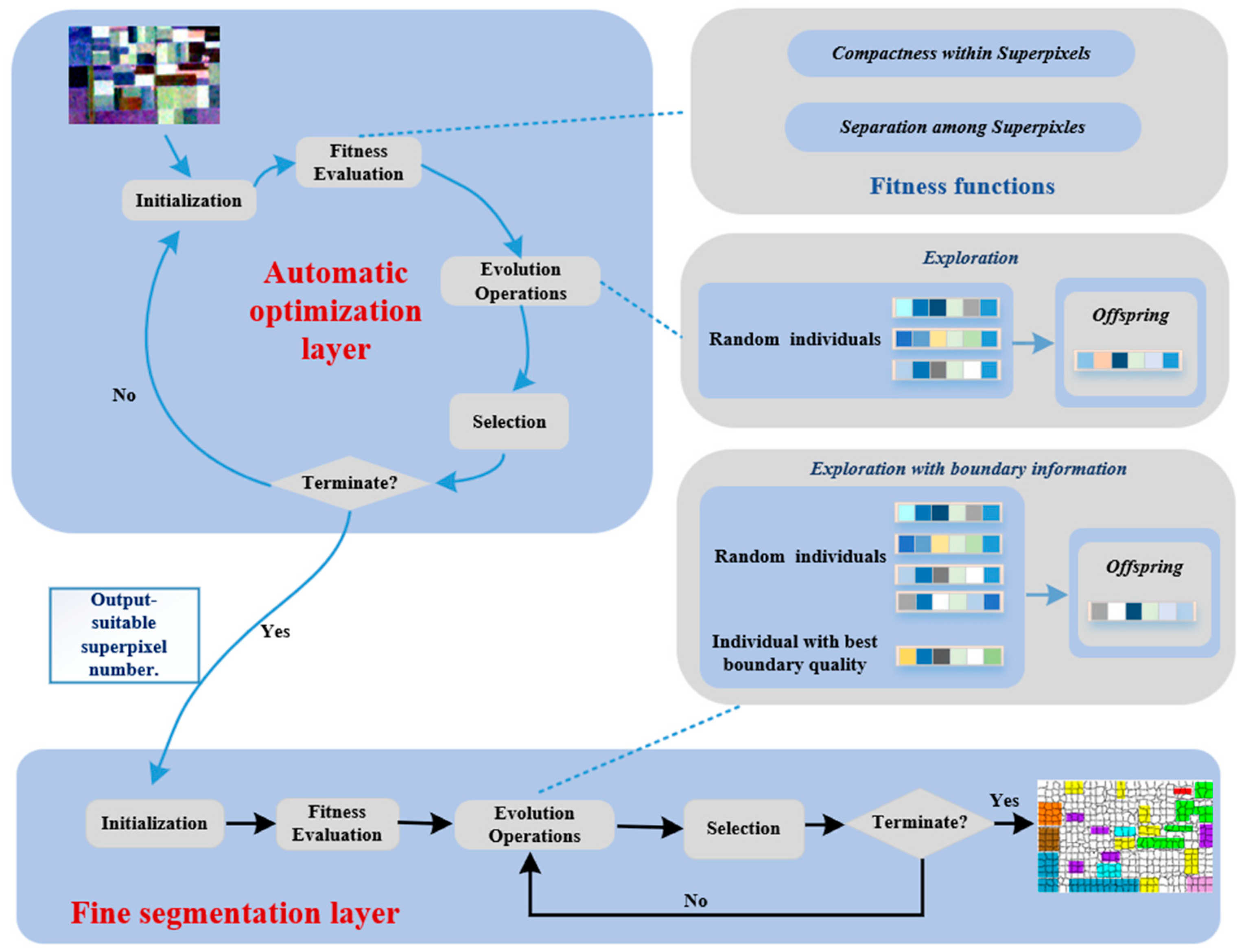
As shown in Figure 1, MOES contains two layers, an automatic optimization layer and a fine segmentation layer. The automatic optimization layer aims to determine the number of superpixels automatically by optimizing the compactness within superpixels and the separation among superpixels simultaneously. On the basis of the output of the automatic optimization layer, the fine segmentation layer pursues high-performance superpixel segmentation by using the boundary information of excellent superpixels in the exploration of evolution.
3.2. Automatic Optimization Layer
As shown in Figure 1, the automatic optimization layer is defined on a multiobjective evolutionary fuzzy clustering for superpixel segmentation. The compactness with superpixels and the separation among superpixels are optimized simultaneously. To determine the superpixel number adaptively, a special individual encoding method is designed, where each superpixel center is controlled by a corresponding activation index.
3.2.1. Fitness Functions
The observed PolSAR image can be represented by , where represents the th element in the pixel set, and represents the total number of pixels in the PolSAR image. The fitness functions can be defined by:
The first objective function represents the sum of weighted distances from the pixels to the superpixel centers, which can maximize the compactness of the superpixels. The second objective function aims to maximize the degrees of separation between the superpixels. represents the maximum number of superpixels. represents a set of superpixel centers, and is the current superpixel number. represents the neighborhood range of pixel . is the initial grid width of each region obtained by dividing the observed PolSAR image into square regions. represents the fuzzy membership degree of the th pixel to the th superpixel center . represents the distance measurements between the pixels and the superpixel centers, which can be calculated by:
In Equation (8), represents the Wishart distance between pixel and the superpixel center . represents the Euclidean spatial distance between pixel and superpixel center . and are the coordinates of the pixel and the superpixel center in the PolSAR image. and are the coordinates of the pixel . and are the coordinates of the superpixel center on the PolSAR image, respectively. is a compact parameter. In Equation (9), and represent the feature vector of pixel and the superpixel center , respectively. shows the trace of the matrix , and represents the determinant of the matrix. In the PolSAR images, each pixel can be represented by a scattering matrix as follows:
where the subscripts and represent the horizontal and vertical polarization, respectively. and represent the energy of the co-polarization. and represent the energy of the cross-polarization. All of them are complexed values. According to the reciprocity theorem, the above equation satisfies the condition of . With the scattering vector , a coherent matrix can be obtained in Equation (12). Then, each pixel can be represented by .
3.2.2. Encoding and Initialization
- (1)
- Individual encoding
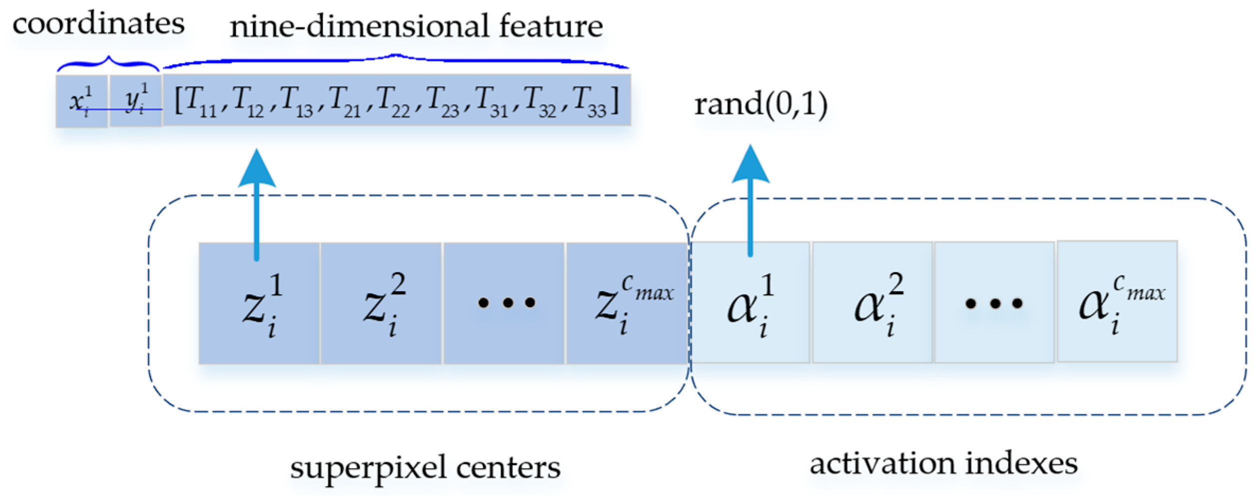
In the automatic optimization layer, each individual in the population is one solution of superpixel segmentation for the observed PolSAR image. Figure 2 shows the individual encoding in the automatic optimization layer. Each individual consists of two parts, the superpixel centers and the activation indexes. The number of superpixel centers is . Each superpixel center is represented by 11 genes, coordinates, and nine-dimensional features. The value range of the activation indexes is . There is a one-to-one correspondence between the superpixel center and the activation index. Only when the activation index is not less than 0.5 is the corresponding superpixel center effective, which is regarded as one candidate superpixel center. Thus, the individuals with the same length in the population have a different number of superpixels.
- (2)
- Population initialization
The population initialization includes the initializations of the activation indexes and the superpixel centers. The activation indexes are initialized randomly within the range of . In the initialization of the superpixel centers, we generate one individual by the centers of square regions of the observed PolSAR image. The superpixel centers of other individuals are initialized by a random pixel within these square regions. Then, all the superpixel centers in each individual are replaced by the pixels with the lowest gradient value in the neighborhood of the current superpixel centers. It is helpful to avoid selecting the pixels in the edges as the superpixel centers.
3.2.3. Evolutionary Operators
- (1)
- Differential evolution strategy
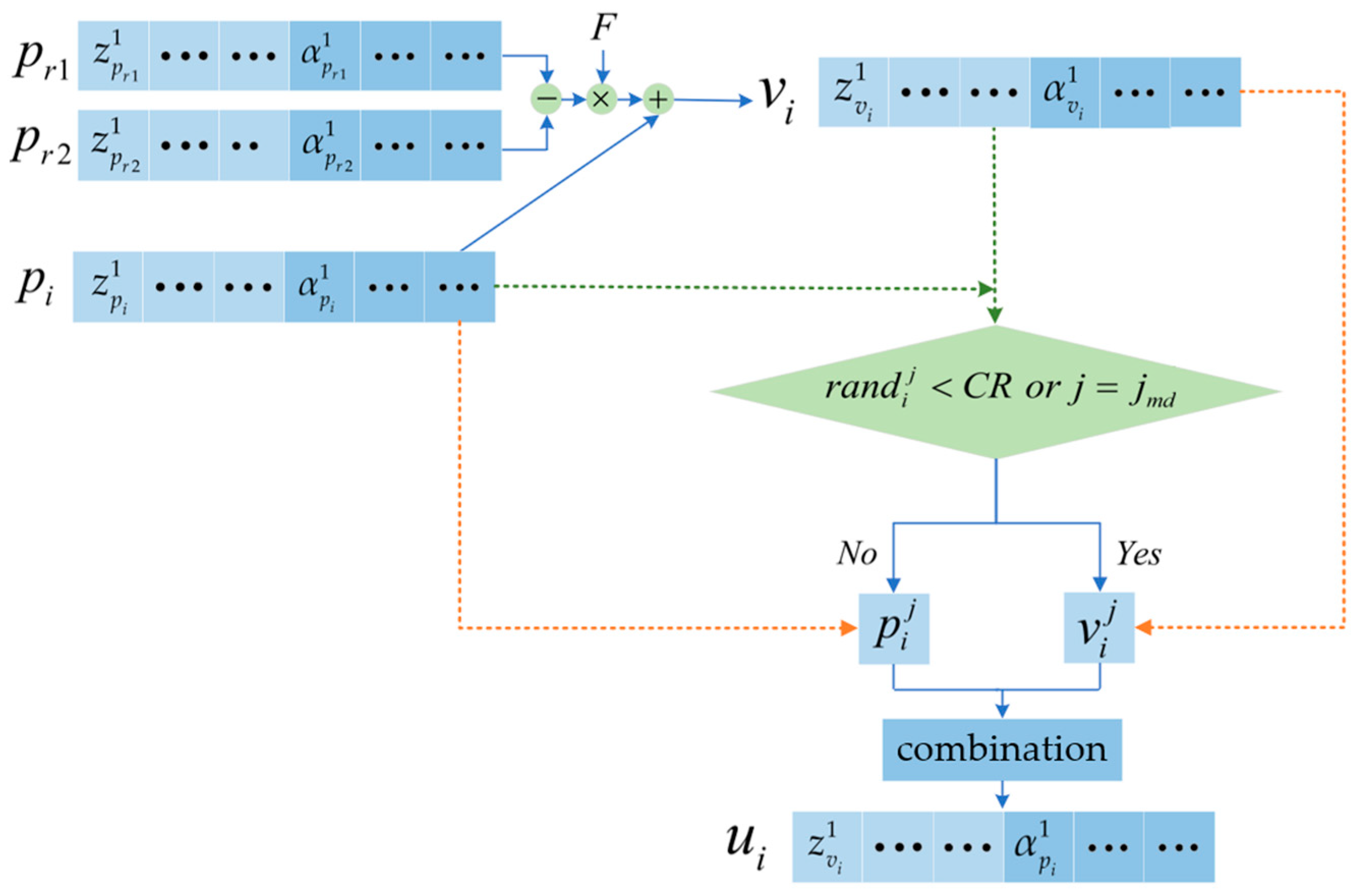
After population initialization, the evolution of the automatic optimization layer starts. The evolutionary operations on the superpixel centers are defined in a differential evolution strategy, as shown in Figure 3. The detailed evolution formulas can be shown as follows:
where represents the th individual in the population. and are two individuals selected randomly from the population. is the mutation coefficient. is the crossover probability. To determine the values of and adaptively, these two parameters can be encoded into individuals, where the values of and are initialized within the range of . Then, these two values can be updated by the evolutionary operators. is the candidate individual generated by three parent individuals in Equation (13). In Equation (14), represents a dimension number selected randomly in advance, which is to ensure the effectiveness of the evolutionary operator. When the random value within is smaller than or the current dimension number equals , the th gene of the new offspring is defined by the th gene of the candidate individual . Then, the corresponding activation index corresponding to the superpixel center also changes by:
where represents the th activation index in the offspring . is a random value between 0 and 1. is a distribution index, which is usually set to 1. If , it means that the superpixel center of the offspring is inherited by the parent individual completely. Then, the corresponding activation index of the offspring is also the same as that of the parent individual .
- (2)
- Individual selection and stop criteria
After the generation of new offspring, the parent individuals and the new offspring are sorted by the non-dominant sorting and the crowding distance in NSGA-II. The better half of all the individuals is selected as the new population. When the generation number of the evolution equals the maximum generation number, the evolution in the automatic optimization layer stops. The individual with the best function is output. With the activation indexes, we can obtain a set of superpixel centers and the exact number of superpixels.
3.3. Fine Segmentation Layer
With the exact number of superpixels, the fine segmentation layer pursues better performance on the basis of the superpixels obtained by the automatic optimization layer. The objective functions in Equations (4)–(7) are still used as the fitness functions in the fine segmentation layer. The encoding strategy and the evolutionary operators are designed to further improve the qualities of superpixels.
3.3.1. Encoding for Fine-Tuning
- (1)
- Individual encoding of fine segmentation layer
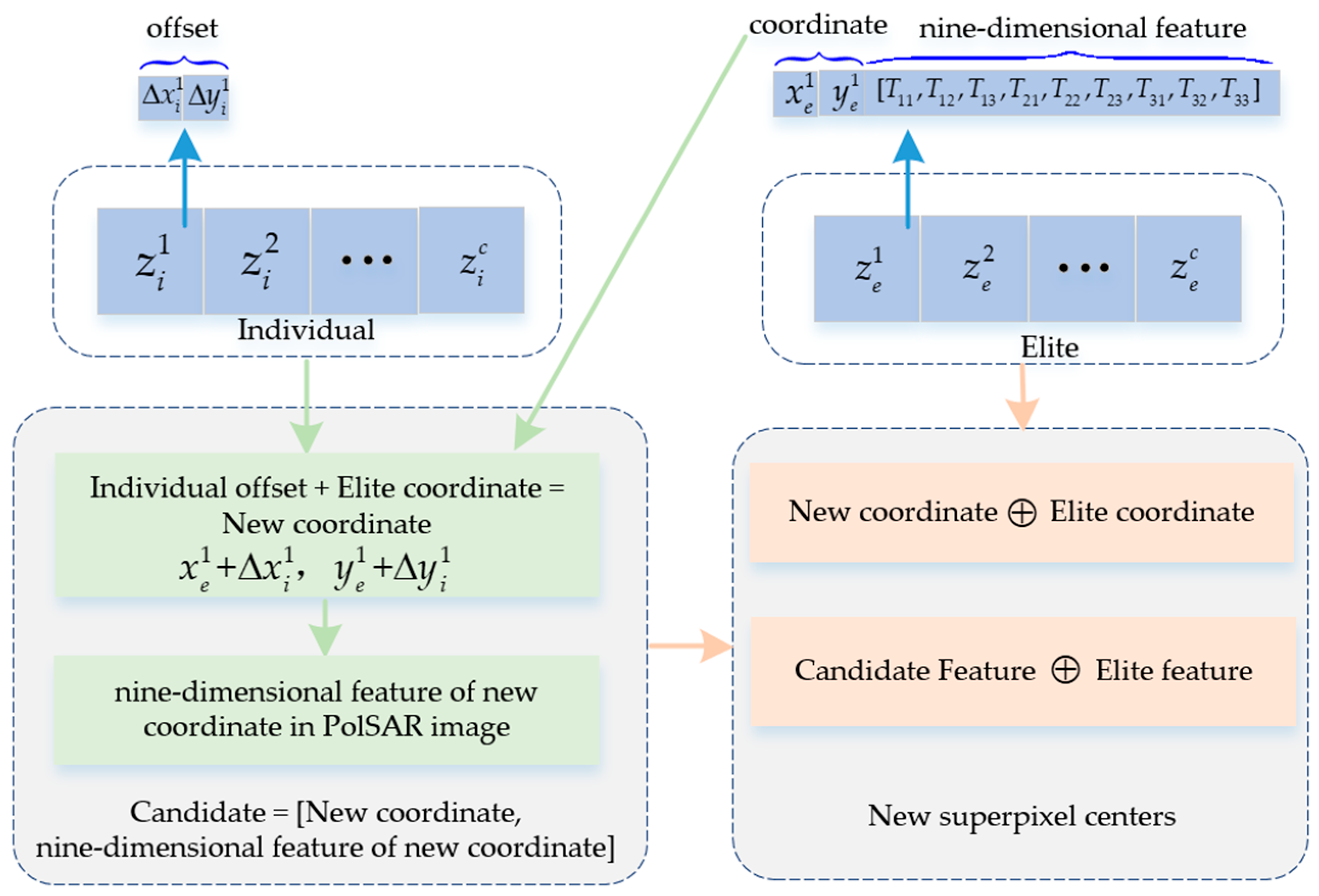
Based on the superpixels obtained by the automatic optimization layer, the search of the fine segmentation layer aims to further improve the qualities of the superpixels. Thus, the encoding strategy is the offset of the coordinates of superpixel centers in the fine segmentation layer. The values of the offset are selected with the range of randomly, where is the grid width of each region obtained by dividing the observed PolSAR image into square regions. As shown in Figure 4, the individual is encoded as a set of coordinates for the superpixel centers, where is the number of superpixels. Let a set of superpixel centers be elite. Combining the offsets of the individual and the coordinates of superpixel centers of the elite, a candidate of superpixel centers can be obtained, which is composed of the new coordinates of superpixel centers and the corresponding features in the PolSAR image. Then, a new set of superpixel centers can be obtained by fine-tuning the elite with the candidate, which can be computed by:
is the th superpixel center by fine-tuning. and are the th superpixel centers of elite and candidate . is the fine-tuning weight, which is set to 0.1.
- (2)
- Population initialization of fine segmentation layer
With the above encoding strategy, we can further perform a search based on the existing superpixels. The initial population is generated randomly in the fine segmentation layer. The initialization of the elite is based on the output individual of the automatic optimization layer. Let the set of the superpixel centers decoded by the output individual of the automatic optimization layer be . The neighbor pixels of the centers of with the lowest gradient values in square regions compose a new set of superpixel centers. We can also obtain a new set of superpixel centers by performing fuzzy c-means (FCM) on , where each pixel may only belong to the superpixel centers in the region around itself. The initial elite is selected as the one with the lowest from the above three sets of superpixel centers. Then, the elite is updated by the individual with the lowest in the evolution of the fine segmentation layer.
3.3.2. Evolutionary Operators of Fine Segmentation Layer
- (1)
- Evolutionary operators with boundary information
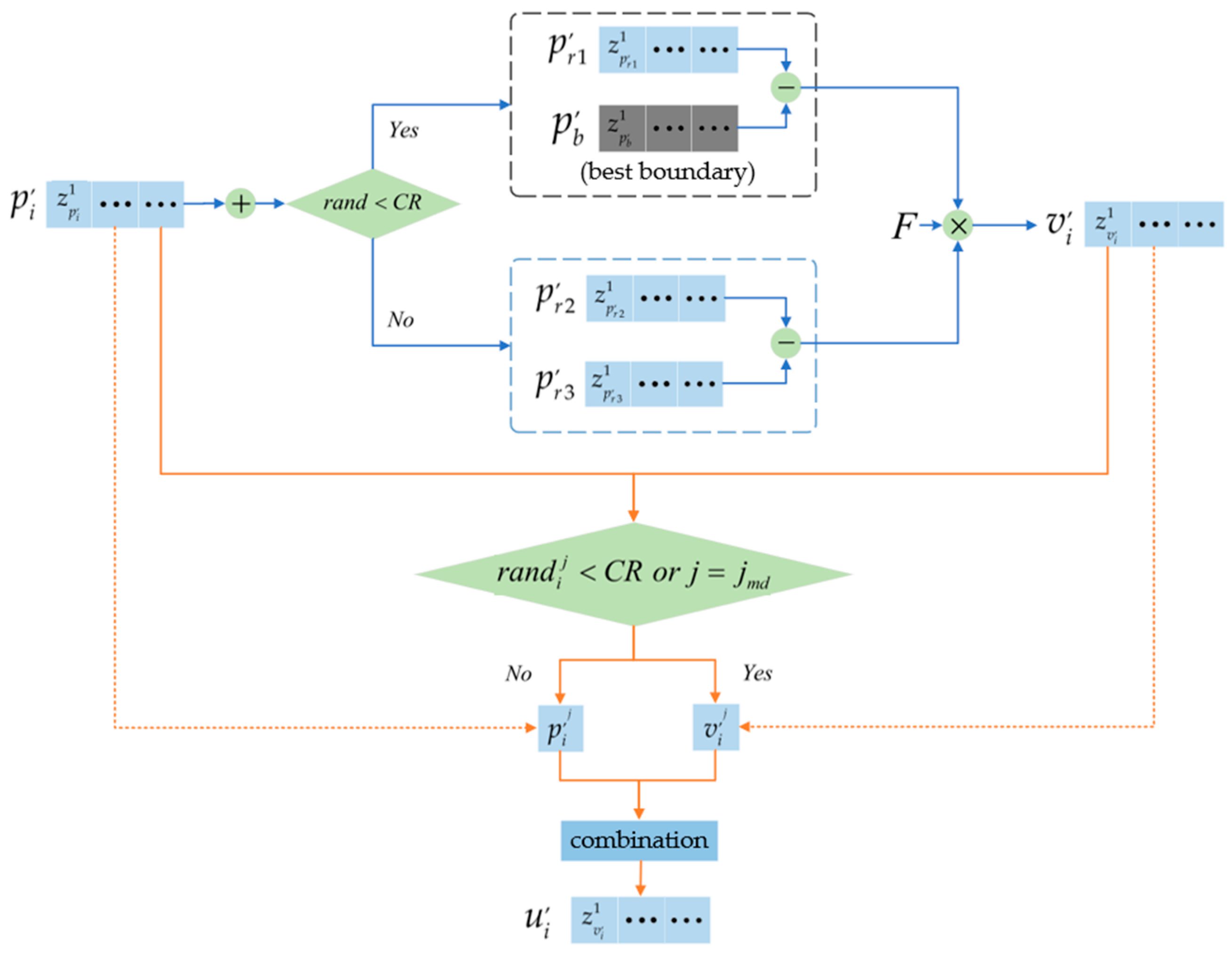
As shown in Figure 5, the evolutionary operator uses the boundary information of superpixels with good qualities in the fine segmentation layer. The detailed evolution formulas are shown as follows:
where represents the th individual in the current population. , , and are three individuals selected randomly from the population, and . and are changed adaptively by the same strategy in the automatic optimization layer.
In Equation (18), the evolutionary operation between the candidate individual and the parent individual to generate the offspring is similar to Equation (14) in the automatic optimization layer. is the individual with the best boundary quality in the population. The boundary quality of each individual can be measured by:
is the gradient value of the th pixel in the observed PolSAR image. represents the real indicator function, where and . indicates the superpixel where the th pixel belongs, and indicates the superpixel where the th neighbor pixel in neighborhood of the th pixel belongs. When the number of the neighbor pixels that belongs to different superpixels is more than two, we set . It indicates that the th pixel may be near or at the boundaries of the superpixels. When the value of is bigger, the boundaries of the superpixels generated by the current individual are closer to the edges of the ground objects in the observed PolSAR images. Thus, we incorporate the individual with the best in the evolutionary operators to improve the boundary quality of the population.
- (2)
- Individual selection and final output
The selection strategy in the fine segmentation layer is the same as the one in the automatic optimization layer. The better individuals are selected from both parent individuals and the new offspring to update the population. When the generation number of the evolution equals the maximum generation number, the evolution stops. The individual with the best function is decoded to obtain the final superpixels.
3.4. Complexity Analysis
In the automatic optimization layer, the population size is , the maximum number of superpixels is , and the total number of pixels in the PolSAR image is . The time complexity of initialization is , and the time complexity of the fitness function calculation is . With the maximum generation number , the time complexity of the automatic optimization layer is . Similarly, the time complexity of the fine segmentation layer is , where is the suitable superpixel number, and and are the population size and the maximum generation number in the fine segmentation layer, respectively. Thus, considering the relationship between the number of pixels and the complexity of the method, the computational complexity of MOES is linear.
4. Experiments Study
4.1. Experiment Settings
4.1.1. PolSAR Datasets
In order to verify the superpixel segmentation performance of MOES, we perform it on three PolSAR datasets, which are Flevoland, Wei River in Xi’an, and San Francisco, respectively.
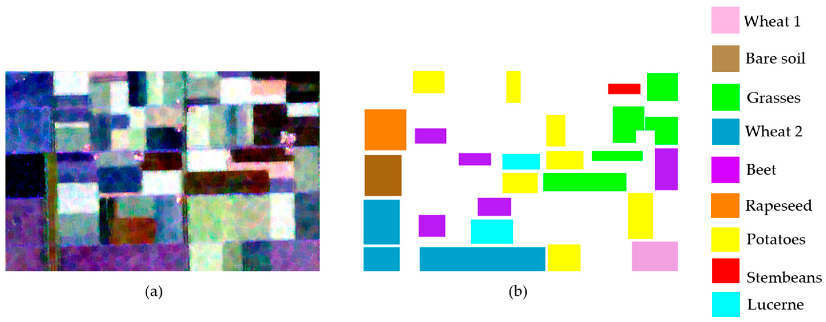
The Flevoland dataset [46] was an L-band multi-view PolSAR image obtained by the AIRSAR airborne platform in 1989, with an image size of 210 × 330 and a resolution of 12 × 6 m. As shown in Figure 6, the scene is Flevoland in the Netherlands, which has recognized ground authenticity to test natural vegetation and land cover. It includes nine crop categories, which are Wheat1, Bare soil, Grasses, Wheat2, Beet, Rapeseed, Potatoes, Stembeans, and Lucerne.
4.1.2. Metrics
In order to better measure the effectiveness of superpixel segmentation, undersegmentation error (UE) and boundary recall (BR) are used as the metrics in this experiment [48]. UE can measure the extent of the areas of the superpixels beyond true ground objects by:
where is the th superpixels, indicates the number of pixels in , and the total number of superpixels is . is the th segment of the ground truth, and the number of segments is . If a superpixel overlaps with more than one segment in ground truth, the value of UE increases. The smaller UE is, the better the quality of the superpixels.
BR represents the degrees of the fits between the boundaries of superpixels and the edges of true ground objects, which can be computed by:
where and are the boundary pixels obtained from the ground truth and the superpixels, respectively. denotes the number of pixels in the boundaries of the ground truth. A large value of BR indicates that the superpixels are not bad quality. In addition, the overall accuracy (OA), average accuracy (AA), and Kappa coefficient are utilized to quantify the classification performance of the superpixels [49].
4.2. Studies on MOES
4.2.1. Parameter Settings
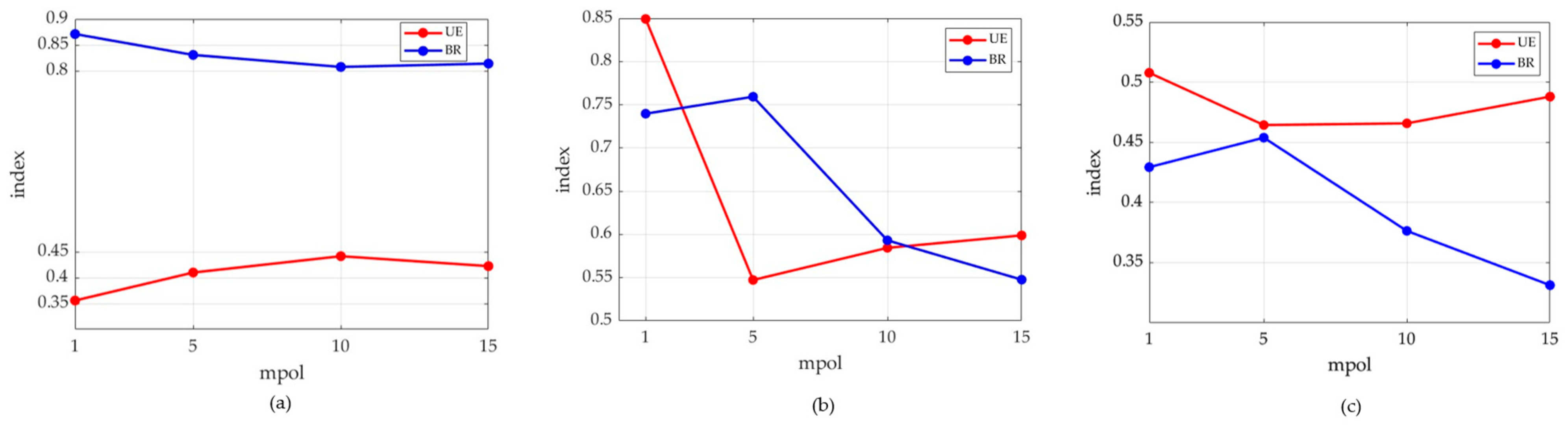
Considering the scales of different scenarios, the values of are set as 800, 1100, and 2000 for the Flevoland dataset, the Wei River in Xi’an dataset, and the San Francisco dataset, respectively. Considering the trade-off between the search ability and computation cost, the population size and the maximum generation number are set as five and ten for both layers in MOES, respectively. Figure 9 shows the sensitivity studies of the parameter in the Wishart distance on different PolSAR datasets. The horizontal coordinate represents the values of , and the vertical coordinate represents the values of UE and BR. The values of are set within the range of , where the interval is five. In Figure 9a, when , the maximum BR and the minimum UE can be obtained on the Flevoland dataset. In Figure 9b,c, MOES performs best in the Wei River in Xi’an dataset and the San Francisco dataset when . It can be seen that the suitable value of changes with different datasets. With the above observations, the values of are set as one and five for the Flevoland dataset and the other two PolSAR datasets, respectively.
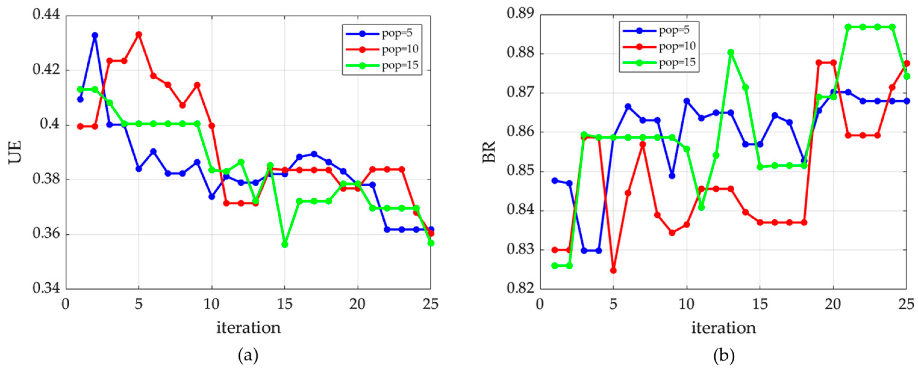
Figure 10 and Figure 11 show the sensitivities of the population sizes and maximum generation numbers in the Flevoland dataset. In Figure 10, the best values of BR and UE obtained by the different values of in the evolution process of the automatic optimization layer are given. We set the population size to 5, 10, and 15, respectively. The maximum generation number is set to 25. The curves of UE and BR are steeper because the automatic optimization layer encodes the superpixel center as individuals directly, which has a relatively significant randomness in the search. With the increase of the iteration number, the UE shows an overall downward trend while BR shows an overall upward trend. It indicates that better solutions appear in the evolution process. Moreover, the curves of UE and BR of the evolution with different population sizes are not significantly different. When the population size and the maximum generation number increase, the computation complexity and the cost time also increase gradually. Considering both the performance and the efficiency, we set the population size and the maximum generation number to five and ten, respectively.
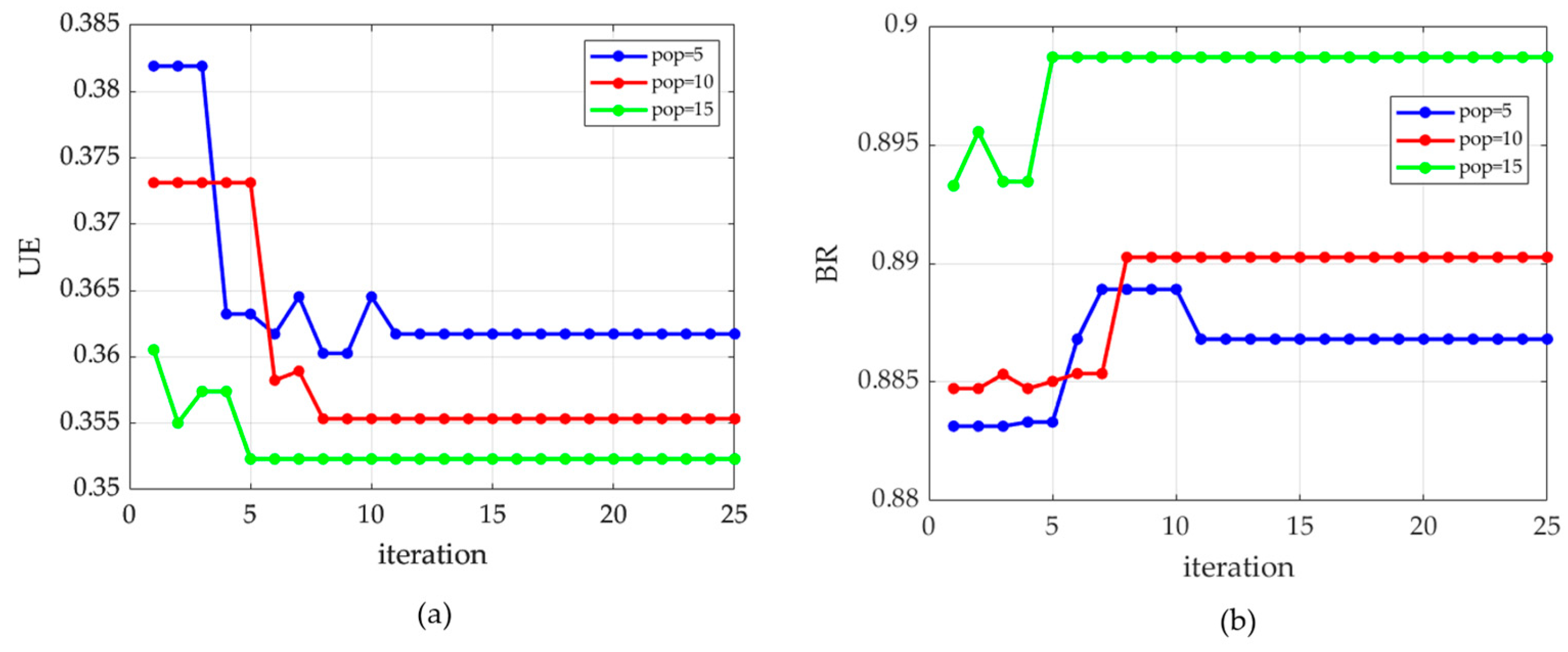
Figure 11 shows the sensitivities of parameters and in the fine segmentation layer. With the increase of the iteration number, the curves of UE present an overall downward trend, while BR presents an overall upward trend. The curves of both UE and BR obtained by three population sizes essentially converge after 10 iterations. The fine segmentation layer is evolved on the basis of the output of the automatic optimization layer, so the convergence speed is faster. When equals 15, UE and BR are the best. Although UE and BR are relatively worse when equals 5, the values of UE and BR are still not bad. In order to ensure the efficiency of MOES, we set the population size and the maximum generation number to five and ten, respectively.
4.2.2. PFs of MOES
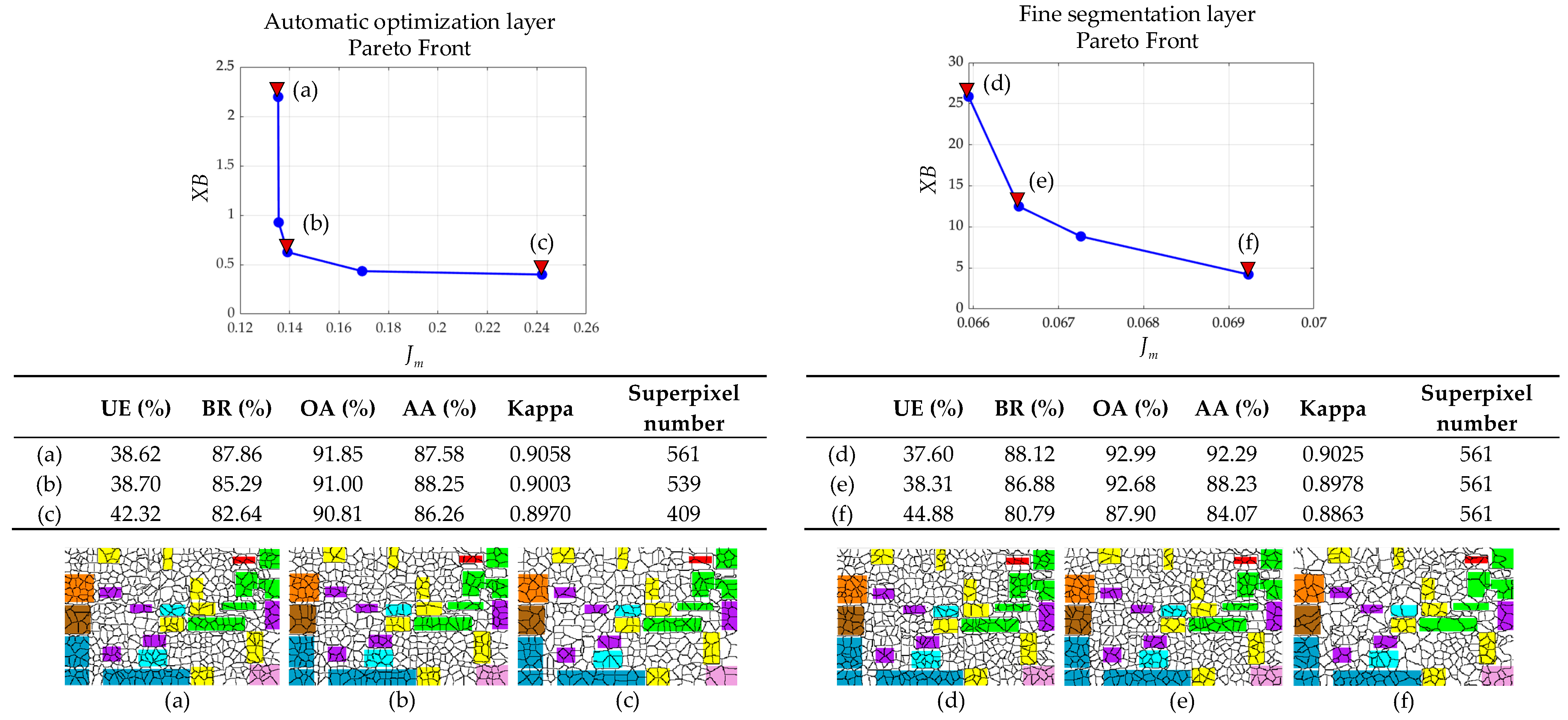
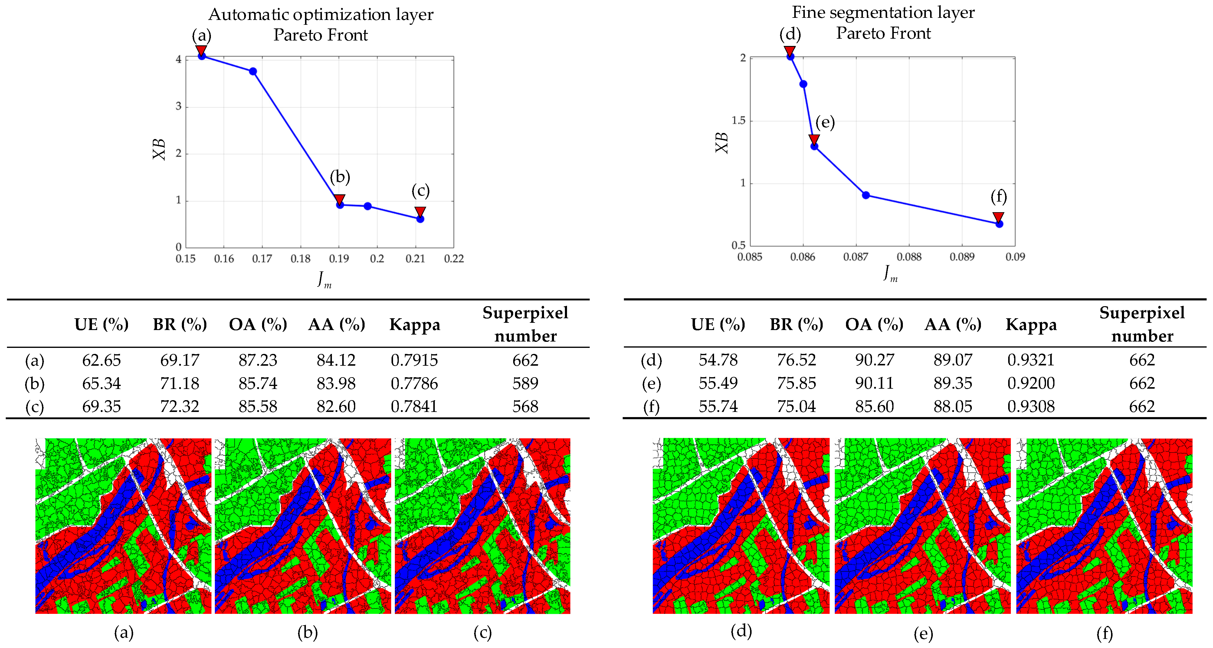
MOES consists of an automatic optimization layer and a fine segmentation layer. Both of these layers feature multiobjective evolution for superpixel segmentation and obtain PFs. In the automatic optimization layer, PF is composed of superpixel segmentations with different superpixel numbers. In the fine segmentation layer, the number of superpixels is fixed, and PF is composed of superpixel segmentations with different performances. Figure 12, Figure 13 and Figure 14 show the PFs obtained by two layers of MOES in three PolSAR datasets.
In Figure 12, the left PF is obtained by the automatic optimization layer in the Flevoland dataset, which is relatively uniform and has good convergence. Additionally, we select three solutions of PF and compare their performances. Obviously, different numbers of superpixels correspond to very different performances. Compared with the other two solutions (b) and (c), solution (a) has the lowest and better performance in both numerical results and visual results. Based on solution (a), the fine segmentation layer obtains the right PF. Compared with solutions (e) and (f), solution (d), with the lowest , achieves better performance in both numerical results and visual results. It validates the effectiveness of selecting the final solution from PF by the lowest value of . Furthermore, it is obvious that the metrics of solutions obtained by the fine segmentation layer are better than the ones obtained by the automatic optimization layer. It indicates that the fine segmentation layer can further improve the qualities of superpixels obtained by the automatic optimization layer.
Figure 13 shows the PFs obtained by MOES in the Wei River in Xi’an dataset. The PF of the automatic optimization layer is not smooth enough. It is a common situation in MOP for practical applications due to the difficulty and complexity of practical problems. Among the three solutions, solution (a), with the lowest , performs best on most of the metrics except for BR. The PF of the fine segmentation layer is uniform and smooth. The solutions make a great improvement in all five metrics on the basis of solution (a), especially solution (d), which has the lowest . Moreover, compared with the visual results obtained by the automatic optimization layer, the superpixels are more regular and uniform in the visual results obtained by the fine segmentation layer.
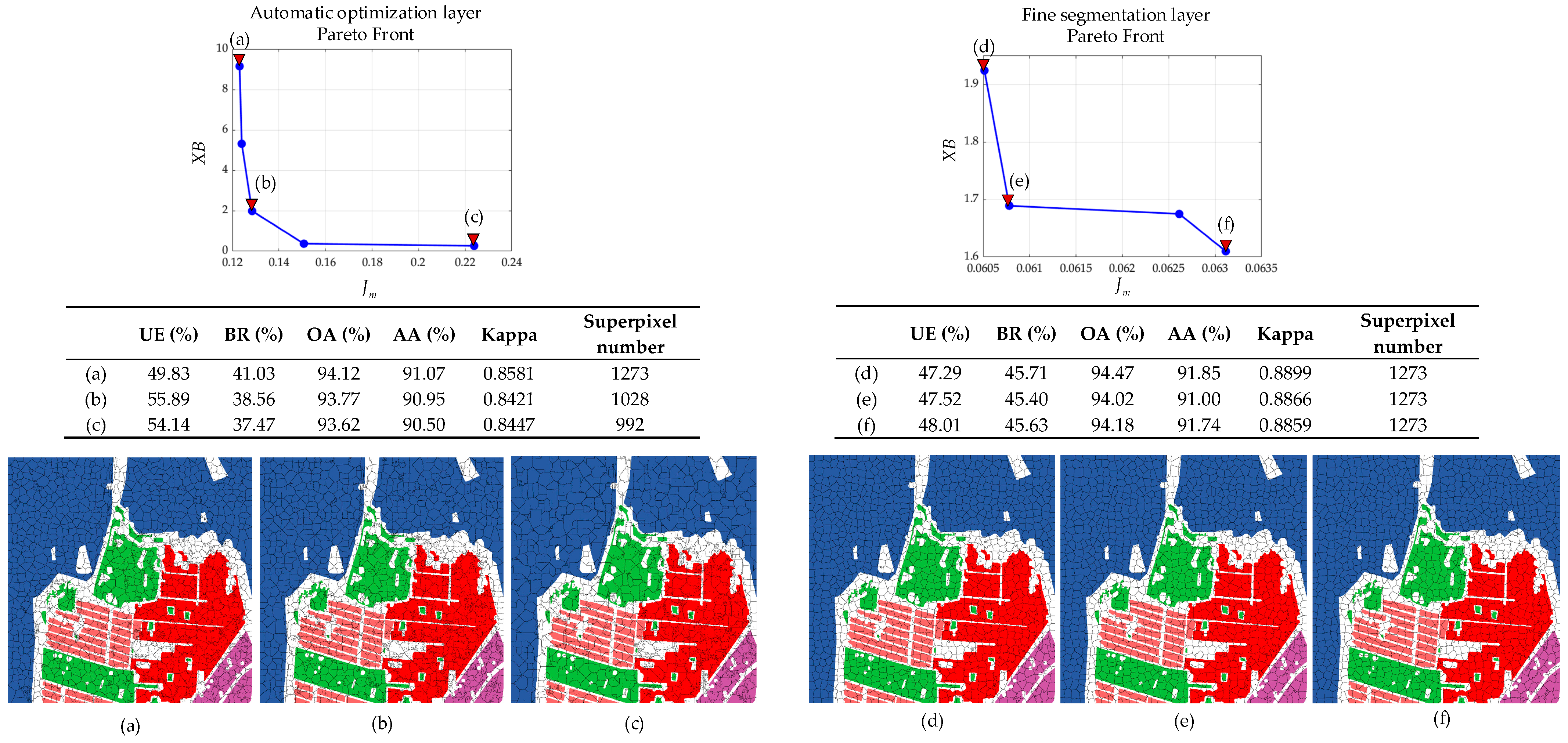
As shown in Figure 14, the PF of the automatic optimization layer in the San Francisco dataset is relatively uniform, where the convergence is good. Among the three solutions, solution (a), with the lowest , has the best performance. Then, the fine segmentation layer obtains more uniform superpixels and better performance, especially solution (d), which has the lowest .
4.2.3. Number of Superpixels in MOES
Unlike the traditional superpixel segmentation techniques, MOES can determine the number of superpixels automatically. Table 1 shows the number of superpixels obtained by MOES over five independent runs in different PolSAR datasets. The number of superpixels in the Flevoland dataset is within the range of 533 to 562. The number of superpixels in the Wei River in Xi’an dataset are within the range of 620 to 668. The maximum and minimum values of the number of superpixels are 1287 and 1217 in the San Francisco dataset, respectively. Obviously, the number of superpixels searched by MOES over different independent runs is stable for each PolSAR dataset.
4.3. Comparison Experiments on PolSAR Datasets
To further study the performance of MOES, we compare it with six popular superpixel segmentation approaches, which are SLIC [9], SEEDS [10], TP [11], QS [14], POL-HLT [50], and HCI [51]. Among them, POL-HLT is a PolSAR superpixel segmentation method with improved SLIC, where an improved initialization and a modified distance metric to Hotelling–Lawley trace distance are introduced. HCI is a PolSAR superpixel segmentation method with modified Wishart distance and geodesic distance for cross-iteration. Due to the randomness of EAs, the mean and standard deviation of numerical results obtained by MOES are reported in the following experiments. Other comparison approaches are performed over five independent runs with five different values of superpixel numbers obtained by MOES, and the best performances are reported as their results. To analyze the relationship between the number of image pixels and the complexity of superpixel segmentation approaches, the computational complexities of all the comparison superpixel algorithms are shown in Table 2.
4.3.1. Comparison Results in Flevoland Dataset
Table 3 and Table 4 give the statistical results of superpixel metrics and classification metrics of all algorithms in the Flevoland dataset. The best metrics in the tables have been bolded. Obviously, MOES has the highest BR and the lowest UE among all the comparison approaches. In Table 4, MOES achieves the best values of AA and Kappa. QS achieves the best OA, but its performance on AA and Kappa is not good enough. The index OA obtained by MOES was 1.73% and 0.09% higher than POL-HLT and HCI, respectively. HCI achieves the best AA, but its OA and Kappa are not good enough. Its UE and BR are also not as good as MOES. MOES performs almost the best in both superpixel segmentation metrics and classification metrics among the comparison approaches in the Flevoland dataset.
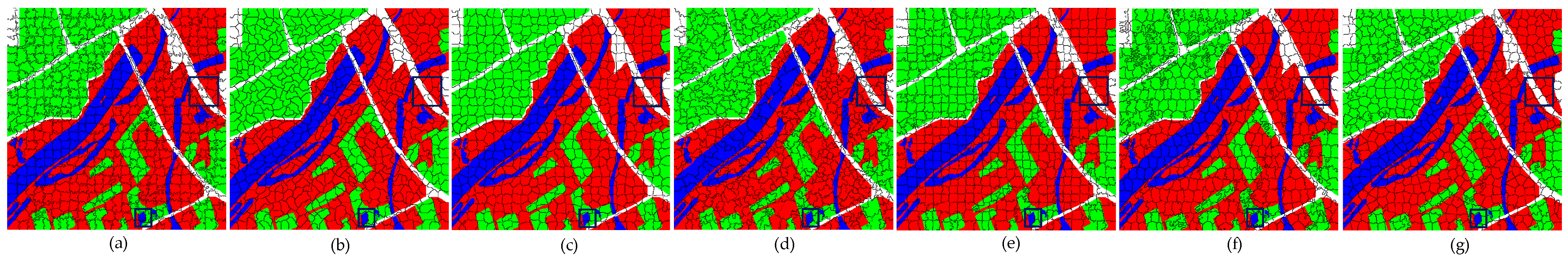
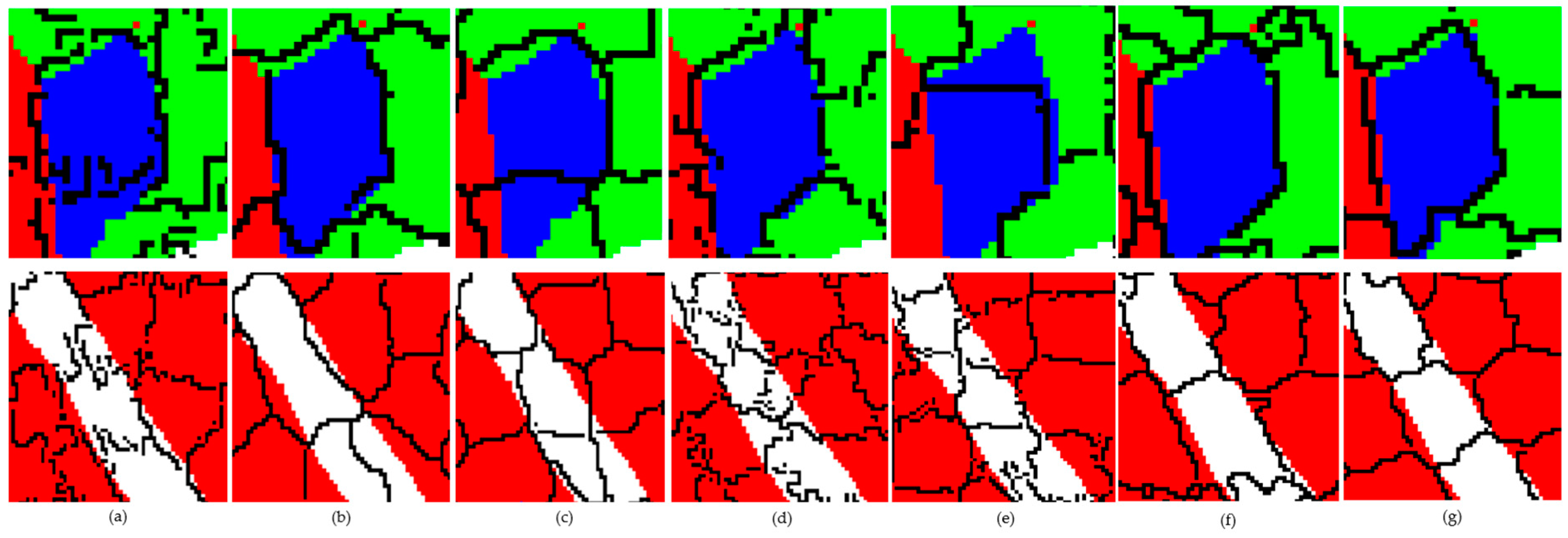
Figure 15 shows the visual results of all algorithms in the Flevoland dataset. In the QS results, the superpixels are very uneven, and the dividing lines are rather tortuous. The match between superpixels and ground objects is not very good. The superpixels generated by SLIC, SEEDS, TP, POL-HLT, and HCI are regular in shape and fit well into each category of ground objects. The dividing lines are also smooth and continuous. Although the shapes of the superpixels generated by MOES are not as regular as those of the previous comparison algorithms, the boundary adhesion is very good, and the dividing line is also very smooth. In order to further observe the qualities of the superpixels, the blue box regions in Figure 11 are enlarged in Figure 16. In the results of SEEDS, TP, and QS, the boundary adhesion is poor, and discontinuity appears. These lead to reduced segmentation performance. The dividing lines obtained by SLIC, POL-HLT, and HCI are relatively smooth, but the boundary adhesion in some regions is still not good enough. In the result of MOES, both the boundary adhesion and the classification performance of MOES are impressive. The dividing lines are also smooth and continuous.
4.3.2. Comparison Results in Wei River in Xi’an Dataset
The statistical results of the superpixel segmentation metrics and classification metrics of all algorithms in the Wei River in Xi’an dataset are shown in Table 5 and Table 6. Both the UE and the BR of MOES are the best. In Table 6, MOES also achieves the best values of OA and Kappa. Although QS has the largest AA, it does not perform well enough in the other two classification metrics, especially Kappa. Furthermore, MOES has the second-best AA. In other words, MOES performs almost the best in both the superpixel segmentation metrics and classification metrics among the comparison approaches in the Wei River in Xi’an dataset.
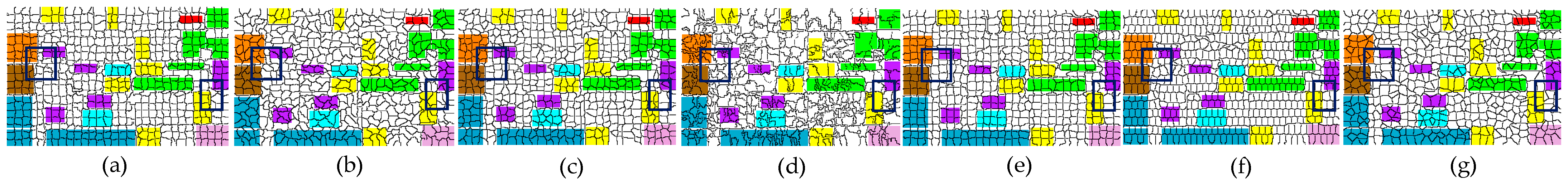
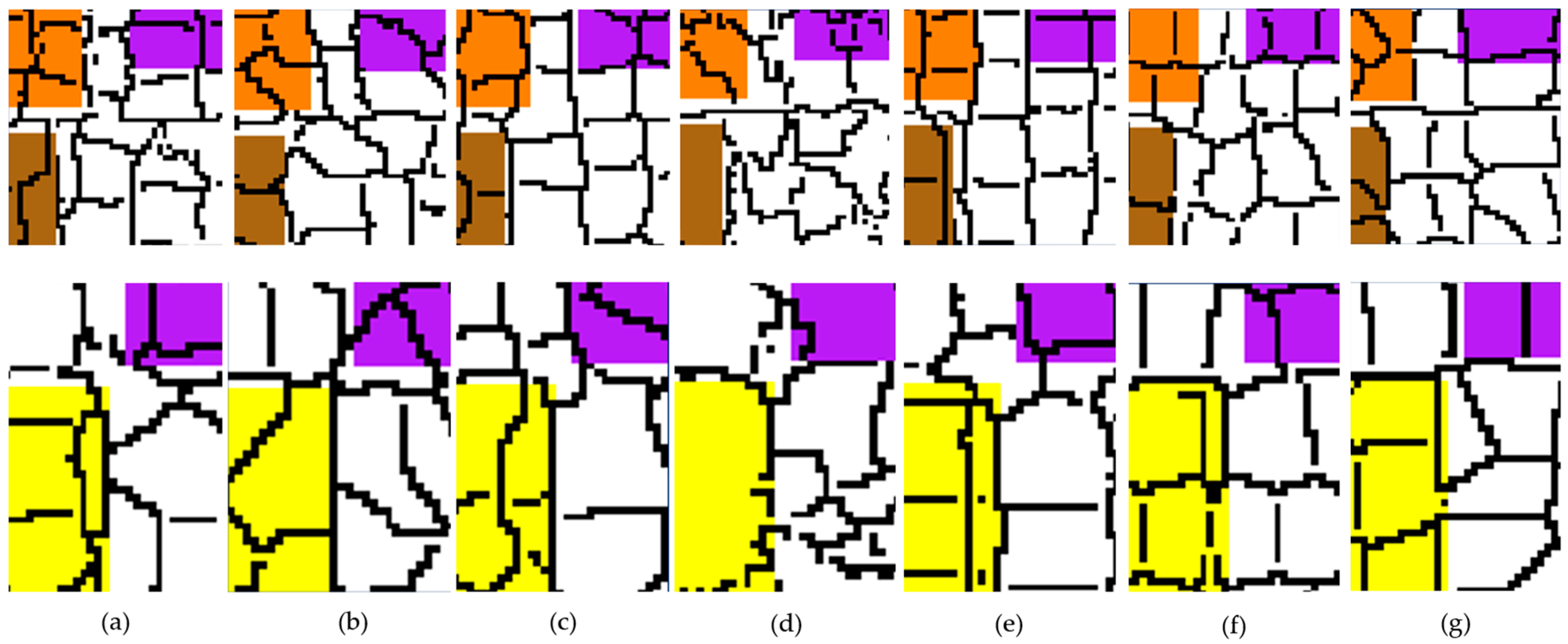
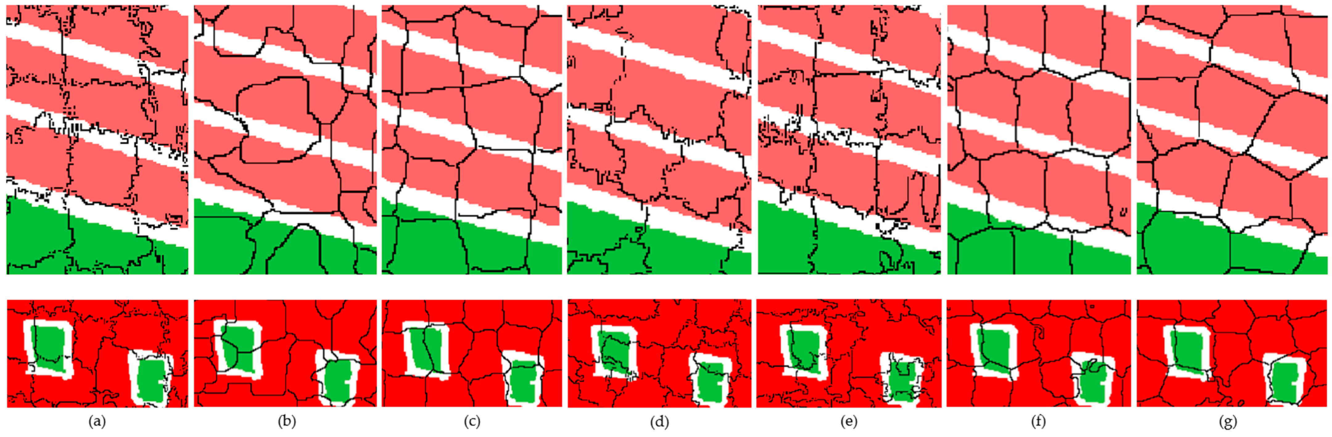
Figure 17 shows the visual superpixel segmentation results of all algorithms in the Wei River in Xi’an dataset. The dividing lines of QS and SLIC are rather tortuous, which results in many discontinuous situations. The generated superpixels of SEEDS and QS are irregular and uneven. The shapes of the superpixels generated by TP and POL-HLT are relatively regular. Their superpixels fit well to each type of ground object, and the dividing lines are also relatively smooth. Although the shapes of superpixels generated by HCI are relatively regular, some small, disconnected regions still exist. The superpixels of MOES are relatively uniform and regular, which fit well with the edges of ground objects. The dividing lines are also relatively smooth. Observing the enlarged regions in Figure 18, the boundary adhesions of SLIC, QS, and POL-HLT are still not good. In the enlarged regions of SEEDS, TP, and HCI, the dividing lines are smooth, and the boundary adhesions are normal. Compared with the above approaches, MOES has better boundary adhesion, more accurate segmentations, and smoother dividing lines. The generated superpixels are also more regular and uniform.
4.3.3. Comparison Results in San Francisco Dataset
As shown in Table 7 and Table 8, the statistical results of superpixel segmentation metrics and classification metrics of all algorithms in the San Francisco dataset are given. MOES has the highest BR, reaching 45.62%, which is 1.42% higher than the second-best comparison algorithm. MOES achieves the second-best UE, which is 0.64% higher than the lowest UE obtained by SLIC. Moreover, the value of BR of MOES is 1.77% higher than the one of SLIC. In Table 8, QS performs the best in OA and AA, while MOES performs the best in Kappa.
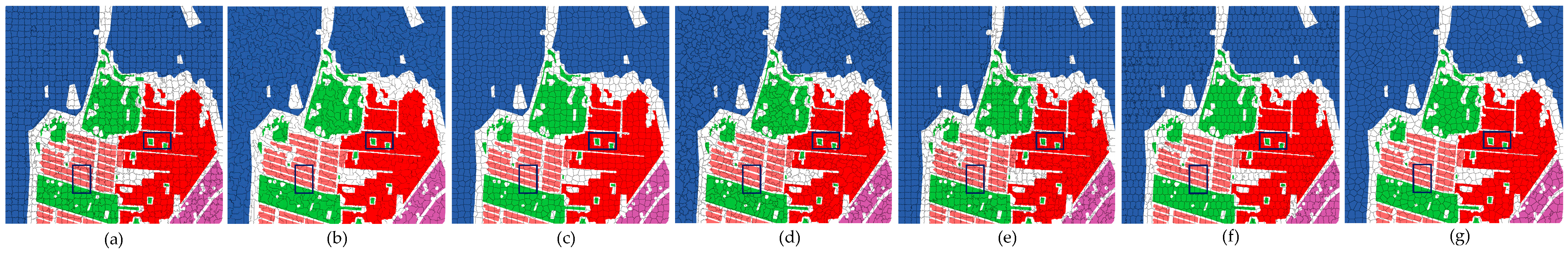
Figure 19 shows the visual superpixel segmentation results of all algorithms in the San Francisco dataset. The division lines of SEEDS and QS are rather tortuous, and the generated superpixels are irregular. Their fittings with the edges of ground objects are not good. The superpixels generated by SLIC, TP, POL-HLT, and HCI are more regular in shape and have smoother dividing lines, but their boundary adhesions are still not good. The superpixels generated by MOES are relatively regular, and the dividing lines are also the smoothest. The boundary adhesion of MOES is similar to those of SLIC, POL-HLT, and HCI. With the observation of the enlarged regions in Figure 20, the dividing lines of SLIC, QS, and POL-HLT are discontinuous. Their boundary adhesions are not good for most ground objects, and the segmentation performances are not good. The boundaries of superpixels of HCI are continuous; its BR index is very low, as seen in Table 7. Although MOES does not fit the edges of the ground objects accurately enough in the boundaries of superpixels, its boundary adhesion is relatively better than the compared algorithms. In addition, the superpixels generated by MOES are relatively uniform, and the dividing lines are relatively smooth.
4.4. Discussion
With the observations of the above experimental results, it can be seen that MOES shows excellent performance on different PolSAR datasets. It can achieve well and balanced performance for different metrics, including the metrics of both superpixel segmentation and classification. The boundaries of superpixels obtained by MOES in the visual results also fit the edges of ground objects relatively well. In the automatic optimization layer of MOES, the number of superpixels can be determined automatically by maximizing the similarities within the superpixels and minimizing the differences among the superpixels simultaneously. It can greatly avoid performance degradation resulting from the manual setting of the unsuitable superpixel number. In the fine segmentation layer of MOES, a fine search is performed for the rough segmentation output by the automatic optimization layer. It makes full use of the boundary information of high-quality superpixels in the evolution to improve the boundary adhesion and segmentation performance. Most of the existing advanced methods are implemented by clustering and adding different mechanisms to improve performances. MOES is also a cluster-based method in essence. However, its unique two-layer optimization structure can not only determine the superpixel number automatically but also further improve the segmentation performance. Moreover, the specific evolutionary operators in MOES can fully search the solution space and generate high-quality individuals.
5. Conclusions
This study proposes a multiobjective evolutionary superpixel segmentation for PolSAR image classification. MOES consists of two layers, an automatic optimization layer and a fine segmentation layer. In the automatic optimization layer, the superpixel segmentation is converted into a multiobjective optimization to take the similarity within superpixels and the difference among superpixels into consideration simultaneously. The number of superpixels can be determined automatically for the observed PolSAR image. In the fine segmentation layer, the segmentation performance can be further improved by the specific evolutionary operators with the boundary information of good-quality superpixels. To validate the performance of MOES, we compare it with several popular superpixel segmentation techniques in different PolSAR datasets. The results show that MOES can determine the suitable number of superpixels automatically and generate high-quality superpixels uniformly for PolSAR images. Although MOES can achieve impressive performance of superpixel segmentation, it is a population-based optimization method and relatively time-consuming. In our future work, we will try to design a specific divide-and-conquer strategy to improve efficiency while maintaining accuracy and extending the applications for large scenes of PolSAR images. Furthermore, MOES can obtain a set of Pareto solutions, but we just select one as our result. Future work will also investigate making full use of the Pareto solutions to further improve the qualities of PolSAR superpixels.
Author Contributions
Conceptualization, M.Z.; Methodology, M.Z.; Software, B.C. and K.M.; Validation, M.Z. and K.M.; Investigation, J.W., J.C. (Jinyong Chen), J.C. (Jie Chen) and H.Z.; Writing—original draft, B.C. and K.M.; Writing—review & editing, M.Z.; Supervision, L.L. All authors have read and agreed to the published version of the manuscript.
Funding
This work was supported in part by the Beijing Institute of Remote Sensing Information under Grant No. MTX20619C226, and in part by the National Natural Science Foundation of China under Grant No. 62176200.
Data Availability Statement
Data are contained within the article.
Conflicts of Interest
The authors declare no conflict of interest.
References
- Ren, S.; Zhou, F. Semi-Supervised Classification for PolSAR Data with Multi-Scale Evolving Weighted Graph Convolutional Network. IEEE J. Sel. Top. Appl. Earth Obs. Remote Sens. 2021, 14, 2911–2927. [Google Scholar] [CrossRef]
- Ganesan, P.G.; Rao, Y. The application of compact polarimetric decomposition algorithms to L-band PolSAR data in agricul-tural areas. Int. J. Remote Sens. 2018, 39, 8337–8360. [Google Scholar]
- Paek, S.W.; Balasubramanian, S.; Kim, S.; Weck, O. Small-Satellite Synthetic Aperture Radar for Continuous Global Biospheric Monitoring: A Review. Remote Sens. 2020, 12, 2546. [Google Scholar] [CrossRef]
- Tan, W.; Sun, B.; Xiao, C.; Huang, P.; Xu, W.; Yang, W. A Novel Unsupervised Classification Method for Sandy Land Using Fully Polarimetric SAR Data. Remote Sens. 2021, 13, 355. [Google Scholar] [CrossRef]
- Li, M.; Zou, H.; Dong, Z.; Wei, J.; Qin, X. Unsupervised classification of PolSAR image based on tensor product graph diffusion. In Proceedings of the 2021 CIE International Conference on Radar, Haikou, China, 15–19 December 2021; pp. 2505–2508. [Google Scholar]
- Liu, B.; Zhang, Z.; Liu, X.; Yu, W. Representation and Spatially Adaptive Segmentation for PolSAR Images Based on Wedgelet Analysis. IEEE Trans. Geosci. Remote Sens. 2015, 53, 4797–4809. [Google Scholar] [CrossRef]
- Liu, Y.; Yu, M.; Li, B.; He, Y. Intrinsic Manifold SLIC: A Simple and Efficient Method for Computing Content-Sensitive Su-perpixels. IEEE Trans. Pattern Anal. Mach. Intell. 2018, 40, 653–666. [Google Scholar] [CrossRef] [PubMed]
- Gong, Y.; Zhou, Y. Differential evolutionary superpixel segmentation. IEEE Trans. Image Process. 2018, 27, 1390–1404. [Google Scholar] [CrossRef] [PubMed]
- Liu, Y.; Yu, C.; Yu, M.; He, Y. Manifold slic: A fast method to compute content-sensitive superpixels. In Proceedings of the 2016 IEEE Conference on Computer Vision and Pattern Recognition, CVPR, Las Vegas, NV, USA, 27–30 June 2016; pp. 651–659. [Google Scholar]
- Bergh, M.; Boix, X.; Gool, L. Seeds: Superpixels extracted via energy-driven sampling. In Proceedings of the 12th European Conference on Computer Vision, ECCV, Florence, Italy, 7–13 October 2012; pp. 298–314. [Google Scholar]
- Levinshtein, A.; Stere, A.; Kutulakos, K.N.; Fleet, D.J.; Dickinson, S.J.; Siddiqi, K. Turbopixels: Fast superpixels using geometric flows. IEEE Trans. Pattern Anal. Mach. Intell. 2009, 31, 2290–2297. [Google Scholar] [CrossRef] [PubMed]
- Li, Z.; Chen, J. Superpixel segmentation using linear spectral clustering. In Proceedings of the 2015 IEEE Conference on Computer Vision and Pattern Recognition, CVPR, Boston, MA, USA, 7–12 June 2015; pp. 1356–1363. [Google Scholar]
- Comaniciu, D.; Meer, P. Mean shift: A robust approach toward feature space analysis. IEEE Trans. Pattern Anal. Mach. Intell. 2002, 24, 603–619. [Google Scholar] [CrossRef]
- Vedaldi, A.; Soatto, S. Quick shift and kernel methods for mode seeking. In Proceedings of the 10th European Conference on Computer Vision (ECCV), Marseille, France, 12–18 October 2008; pp. 705–718. [Google Scholar]
- Weikersdorfer, D.; Gossow, D.; Beetz, M. Depth-adaptive superpixels. In Proceedings of the 21th International Conference on Pattern Recognition, ICPR, Tsukuba, Japan, 11–15 November 2012; pp. 2087–2090. [Google Scholar]
- Shi, J.; Malik, J. Normalized cuts and image segmentation. IEEE Trans. Pattern Anal. Mach. Intell. 2000, 22, 888–905. [Google Scholar]
- Felzenszwalb, P.F.; Huttenlocher, D.P. Efficient graph-based image segmentation. Int. J. Comput. Vis. 2004, 59, 167–181. [Google Scholar] [CrossRef]
- Tang, D.; Fu, H.; Cao, X. Topology preserved regular superpixel. In Proceedings of the 2012 IEEE International Conference on Multimedia and Expo, Melbourne, VIC, Australian, 9–13 July 2012; pp. 765–768. [Google Scholar]
- Shen, j.; Du, Y.; Wang, W.; Li, X. Lazy random walks for superpixel segmentation. IEEE Trans. Image Process. 2014, 23, 1451–1462. [Google Scholar] [CrossRef] [PubMed]
- Qin, F.; Guo, J.; Lang, F. Superpixel Segmentation for Polarimetric SAR Imagery Using Local Iterative Clustering. IEEE Geosci. Remote Sens. Lett. 2015, 12, 13–17. [Google Scholar]
- Ersahin, K.; Cumming, I.G.; Ward, R.K. Segmentation and Classification of Polarimetric SAR Data Using Spectral Graph Partitioning. IEEE Trans. Geosci. Remote Sens. 2010, 48, 164–174. [Google Scholar] [CrossRef]
- Xiang, D.; Ban, Y.; Wang, W.; Su, Y. Adaptive Superpixel Generation for Polarimetric SAR Images with Local Iterative Clus-tering and SIRV Model. IEEE Trans. Geosci. Remote Sens. 2017, 55, 3115–3131. [Google Scholar] [CrossRef]
- Yang, S.; Yaun, X. Superpixel generation for polarimetric SAR using hierarchical energy maximization. Comput. Geosci. 2020, 135, 104395. [Google Scholar] [CrossRef]
- Lang, F.; Yang, J.; Yan, S.; Qin, F. Superpixel segmentation of polarimetric synthetic aperture radar (sar) images based on generalized mean shift. Remote Sens. 2018, 10, 1592. [Google Scholar] [CrossRef]
- Liu, B.; Hu, H.; Wang, H. Superpixel-based classification with an adaptive number of classes for polarimetric SAR images. IEEE Trans. Geosci. Remote Sens. 2012, 51, 907–924. [Google Scholar] [CrossRef]
- Wang, W.; Xiang, D.; Ban, Y. Superpixel segmentation of polarimetric SAR images based on integrated distance measure and entropy rate method. IEEE J. Sel. Top. Appl. Earth Obs. Remote Sens. 2017, 10, 4045–4058. [Google Scholar] [CrossRef]
- Liu, H.; Yang, S.; Gou, S. Fast classification for large polarimetric SAR data based on refined spatial-anchor graph. IEEE Geosci. Remote Sens. Lett. 2017, 14, 1589–1593. [Google Scholar] [CrossRef]
- Hou, B.; Yang, C.; Ren, B.; Jiao, L. Decomposition-Feature-Iterative-Clustering-Based Superpixel Segmentation for PolSAR Image Classification. IEEE Geosci. Remote Sens. Lett. 2018, 15, 1239–1243. [Google Scholar] [CrossRef]
- Li, M.; Zou, H.; Qin, X.; Dong, Z.; Wei, J. Superpixel Segmentation for PolSAR Images Based on Cross Iteration. In Proceedings of the 2021 IEEE International Geoscience and Remote Sensing Symposium (IGARSS), Brussels, Belgium, 11–16 July 2021; pp. 4739–4742. [Google Scholar]
- Guo, Y.; Jiao, L.; Qu, R.; Sun, Z.; Wang, S. Adaptive Fuzzy Learning Superpixel Representation for PolSAR Image Classification. IEEE Trans. Geosci. Remote Sens. 2022, 60, 5217818. [Google Scholar] [CrossRef]
- Wang, Z.; Zhang, Q.; Zhou, A.; Gong, M.; Jiao, L. Adaptive Replacement Strategies for MOEA/D. IEEE Trans. Cybern. 2016, 46, 474–486. [Google Scholar] [CrossRef]
- Wang, Q.; Guidolin, M.; Savic, D.; Kapelan, Z. Two-Objective Design of Benchmark Problems of a Water Distribution System via MOEAs: Towards the Best-Known Approximation of the True Pareto Front. J. Water Resour. Plan. Manag. 2014, 141, 04014060. [Google Scholar] [CrossRef]
- Nada, M.A. Evolutionary Algorithm Definition. Am. J. Eng. Appl. Sci. 2009, 2, 789–795. [Google Scholar]
- Wang, J.; Peng, H.; Shi, P. An optimal image watermarking approach based on a multiobjective genetic algorithm. Inf. Sci. 2011, 181, 5501–5514. [Google Scholar] [CrossRef]
- Sen, S.; Tang, G.; Nehorai, A. Multiobjective Optimization of OFDM Radar Waveform for Target Detection. IEEE Trans. Signal Process. 2011, 59, 639–652. [Google Scholar] [CrossRef]
- Wagner, T.; Beume, N.; Naujoks, B. Pareto-, aggregation-, and indicator-based methods in many-objective optimization. In Proceedings of the 4th International Conference on Evolutionary Multi-Criterion Optimization (EMO), Matsushima, Japan, 5–8 March 2007; pp. 742–756. [Google Scholar]
- Deb, K.; Pratap, A.; Agarwal, S.; Meyarivan, T. A fast and elitist multiobjective genetic algorithm: NSGA-II. IEEE Trans. Evol. Comput. 2002, 6, 182–197. [Google Scholar] [CrossRef]
- Ishibuchi, H.; Sakane, Y.; Tsukamoto, N.; Nojima, Y. Simultaneous use of different scalarizing functions in MOEA/D. In Proceedings of the 12th annual Conference on Genetic and Evolutionary Computation, Portland, OR, USA, 7–11 July 2010; pp. 519–526. [Google Scholar]
- Zhang, Q.; Li, H. MOEA/D: A multiobjective evolutionary algorithm based on decomposition. IEEE Trans. Evol. Comput. 2007, 11, 712–731. [Google Scholar] [CrossRef]
- Naujoks, B.; Beume, N.; Emmerich, M. Multiobjective optimisation using S-metric selection: Application to three-dimensional solution spaces. In Proceedings of the 2005 IEEE Congress on Evolutionary Computation, Edinburgh, UK, 2–5 September 2005; pp. 1282–1289. [Google Scholar]
- Zhang, M.; Jiao, L.; Ma, W.; Ma, J.; Gong, M. Multiobjective evolutionary fuzzy clustering for image segmentation with MOEA/D. Appl. Soft Comput. 2016, 48, 621–637. [Google Scholar] [CrossRef]
- Zhang, M.; Jiao, L.; Shang, R.; Zhang, X.; Li, L. Unsupervised EA-Based Fuzzy Clustering for Image Segmentation. IEEE Access 2020, 8, 8627–8647. [Google Scholar] [CrossRef]
- Zhong, Y.; Zhang, S.; Zhang, L. Automatic Fuzzy Clustering Based on Adaptive Multiobjective Differential Evolution for Remote Sensing Imagery. IEEE J. Sel. Top. Appl. Earth Obs. Remote Sens. 2013, 6, 2290–2301. [Google Scholar] [CrossRef]
- Hinojosa, S.; Oliva, D.; Pajares, G. Reducing overlapped pixels: A multiobjective color thresholding approach. Soft Comput. 2020, 24, 6787–6807. [Google Scholar] [CrossRef]
- Sağ, T.; Çunkaş, M. Color image segmentation based on multiobjective artificial bee colony optimization. Appl. Soft Comput. 2015, 34, 389–401. [Google Scholar] [CrossRef]
- Ren, B.; Hou, B.; Zhao, J.; Jiao, L. Sparse Subspace Clustering-Based Feature Extraction for PolSAR Imagery Classification. Remote Sens. 2018, 10, 391. [Google Scholar] [CrossRef]
- Chen, Y.; Jiao, L.; Li, Y.; Zhao, J. Multilayer projective dictionary pair learning and sparse autoencoder for PolSAR image classification. IEEE Trans. Geosci. Remote Sens. 2017, 55, 6683–6694. [Google Scholar] [CrossRef]
- Guo, Y.; Jiao, L.; Wang, S.; Wang, S.; Liu, F.; Hua, W. Fuzzy superpixels for polarimetric SAR images classification. IEEE Trans. Fuzzy Syst. 2018, 26, 2846–2860. [Google Scholar] [CrossRef]
- Cohen, J. A coefficient of agreement for nominal scales. Educ. Psychol. Meas. 1960, 20, 37–46. [Google Scholar] [CrossRef]
- Yin, J.; Wang, T.; Du, Y.; Liu, X.; Zhou, L.; Yang, J. SLIC Superpixel Segmentation for Polarimetric SAR Images. IEEE Trans. Geosci. Remote Sens. 2021, 60, 5201317. [Google Scholar] [CrossRef]
- Li, M.; Zou, H.; Qin, X. Efficient Superpixel Generation for Polarimetric SAR Images with Cross-Iteration and Hexagonal Initialization. Remote Sens. 2022, 14, 2914. [Google Scholar] [CrossRef]
Figure 1.
Overall framework of MOES.

Figure 2.
Individual encoding.

Figure 3.
Differential evolution strategy.

Figure 4.
Individual encoding and production of new superpixel centers.

Figure 5.
Evolutionary operator with boundary information.

Figure 6.
Flevoland dataset. (a) Flevoland image (PauliRGB); (b) ground truth.

Figure 7.
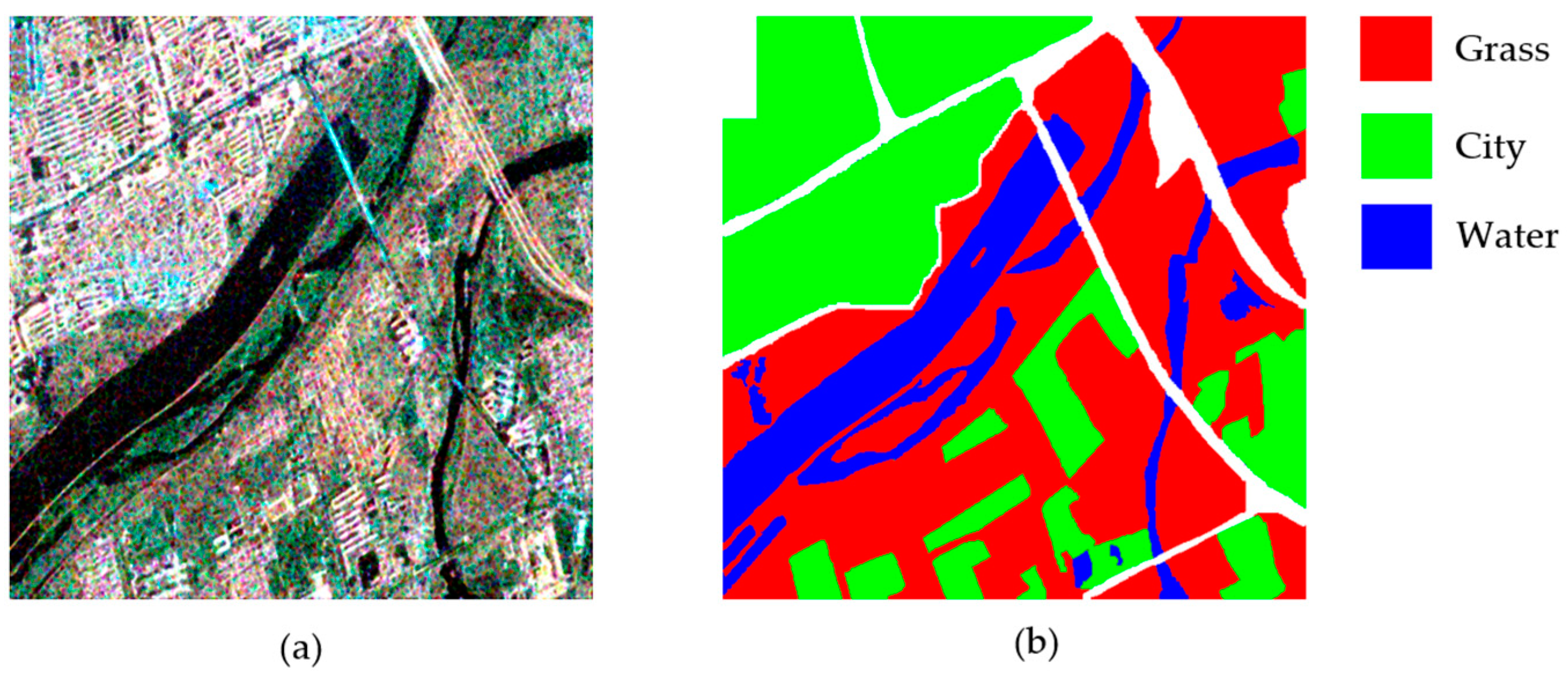
Wei River in Xi’an dataset. (a) Wei River in Xi’an image (PauliRGB); (b) ground truth.

Figure 8.
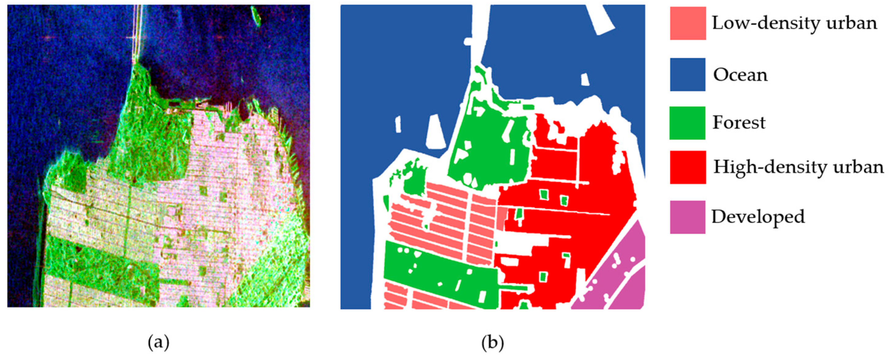
San Francisco dataset. (a) San Francisco image (PauliRGB); (b) ground truth.

Figure 9.
Sensitivity of parameter on different PolSAR datasets. (a) Flevoland dataset; (b) Wei River in Xi’an dataset; (c) San Francisco dataset.
Figure 9.
Sensitivity of parameter on different PolSAR datasets. (a) Flevoland dataset; (b) Wei River in Xi’an dataset; (c) San Francisco dataset.

Figure 10.
Sensitivities of parameters and in automatic optimization layer in Flevoland dataset. (a) UE; (b) BR.
Figure 10.
Sensitivities of parameters and in automatic optimization layer in Flevoland dataset. (a) UE; (b) BR.

Figure 11.
Sensitivities of parameters and in fine segmentation layer in Flevoland dataset. (a) UE; (b) BR.
Figure 11.
Sensitivities of parameters and in fine segmentation layer in Flevoland dataset. (a) UE; (b) BR.

Figure 12.
PFs of two layers of MOES in Flevoland dataset.

Figure 13.
PFs of two layers of MOES in Wei River in Xi’an dataset.

Figure 14.
PFs of two layers of MOES in San Francisco dataset.

Figure 15.
Visual superpixel segmentation results in Flevoland dataset. (a) SLIC; (b) SEEDS; (c) TP; (d) QS; (e) POL-HLT; (f) HCI; (g) MOES.
Figure 15.
Visual superpixel segmentation results in Flevoland dataset. (a) SLIC; (b) SEEDS; (c) TP; (d) QS; (e) POL-HLT; (f) HCI; (g) MOES.

Figure 16.
The enlarged images of the selected regions in visual results in Flevoland dataset. (a) SLIC; (b) SEEDS; (c) TP; (d) QS; (e) POL-HLT; (f) HCI; (g) MOES.
Figure 16.
The enlarged images of the selected regions in visual results in Flevoland dataset. (a) SLIC; (b) SEEDS; (c) TP; (d) QS; (e) POL-HLT; (f) HCI; (g) MOES.

Figure 17.
Visual superpixel segmentation results in Wei River in Xi’an dataset. (a) SLIC; (b) SEEDS; (c) TP; (d) QS; (e) POL-HLT; (f) HCI; (g) MOES.
Figure 17.
Visual superpixel segmentation results in Wei River in Xi’an dataset. (a) SLIC; (b) SEEDS; (c) TP; (d) QS; (e) POL-HLT; (f) HCI; (g) MOES.

Figure 18.
The enlarged images of the selected regions in visual results in Wei River in Xi’an dataset. (a) SLIC; (b) SEEDS; (c) TP; (d) QS; (e) POL-HLT; (f) HCI; (g) MOES.
Figure 18.
The enlarged images of the selected regions in visual results in Wei River in Xi’an dataset. (a) SLIC; (b) SEEDS; (c) TP; (d) QS; (e) POL-HLT; (f) HCI; (g) MOES.

Figure 19.
Visual superpixel segmentation results in San Francisco dataset. (a) SLIC; (b) SEEDS; (c) TP; (d) QS; (e) POL-HLT; (f) HCI; (g) MOES.
Figure 19.
Visual superpixel segmentation results in San Francisco dataset. (a) SLIC; (b) SEEDS; (c) TP; (d) QS; (e) POL-HLT; (f) HCI; (g) MOES.

Figure 20.
The enlarged images of the selected regions in visual results in San Francisco dataset. (a) SLIC; (b) SEEDS; (c) TP; (d) QS; (e) POL-HLT; (f) HCI; (g) MOES.
Figure 20.
The enlarged images of the selected regions in visual results in San Francisco dataset. (a) SLIC; (b) SEEDS; (c) TP; (d) QS; (e) POL-HLT; (f) HCI; (g) MOES.


Table 1.
The numbers of superpixels obtained by running MOES five times in three datasets.
| Independent Run | Flevoland | Wei River in Xi’an | San Francisco |
|---|---|---|---|
| 1 | 533 | 642 | 1271 |
| 2 | 554 | 659 | 1253 |
| 3 | 544 | 620 | 1273 |
| 4 | 561 | 662 | 1217 |
| 5 | 562 | 668 | 1287 |
Table 2.
Computational complexity of superpixel segmentation algorithms.
| SLIC | SEEDS | TP | QS | POL-HLT | HCI | MOES |
|---|---|---|---|---|---|---|
Table 3.
Statistical results of superpixel metrics of all algorithms in Flevoland dataset.
| Index | SLIC | SEEDS | TP | QS | POL-HLT | HCI | MOES |
|---|---|---|---|---|---|---|---|
| UE (%) | 39.26 | 40.88 | 36.85 | 42.83 | 37.86 | 37.02 | 36.72 ± 0.81 |
| BR (%) | 86.81 | 88.10 | 86.18 | 83.62 | 87.13 | 88.45 | 89.04 ± 0.99 |
Table 4.
Statistical results of classification metrics of all algorithms in Flevoland dataset.
| Index | SLIC | SEEDS | TP | QS | POL-HLT | HCI | MOES |
|---|---|---|---|---|---|---|---|
| OA (%) | 93.72 | 93.05 | 92.98 | 94.66 | 91.25 | 92.89 | 92.98 ± 0.57 |
| AA (%) | 90.87 | 91.14 | 91.95 | 89.05 | 92.09 | 93.13 | 92.49 ± 0.17 |
| Kappa | 0.9063 | 0.9015 | 0.9025 | 0.8831 | 0.8960 | 0.9069 | 0.9258 ± 0.03 |
Table 5.
Statistical results of superpixel metrics of all algorithms in Wei River in Xi’an dataset.
| Index | SLIC | SEEDS | TP | QS | POL-HLT | HCI | MOES |
|---|---|---|---|---|---|---|---|
| UE (%) | 58.53 | 55.59 | 55.05 | 62.86 | 59.01 | 57.68 | 55.04 ± 0.87 |
| BR (%) | 74.94 | 66.37 | 64.46 | 75.68 | 64.19 | 73.57 | 76.95 ± 0.65 |
Table 6.
Statistical results of classification metrics of all algorithms in Wei River in Xi’an dataset.
Table 6.
Statistical results of classification metrics of all algorithms in Wei River in Xi’an dataset.
| Index | SLIC | SEEDS | TP | QS | POL-HLT | HCI | MOES |
|---|---|---|---|---|---|---|---|
| OA (%) | 89.75 | 88.85 | 89.99 | 89.71 | 88.02 | 89.03 | 90.30 ± 0.10 |
| AA (%) | 89.04 | 87.94 | 89.28 | 89.66 | 87.15 | 87.94 | 89.37 ± 0.21 |
| Kappa | 0.8311 | 0.8288 | 0.8309 | 0.8224 | 0.8096 | 0.8194 | 0.8941 ± 0.02 |
Table 7.
Statistical results of superpixel metrics of all algorithms in San Francisc dataset.
| Index | SLIC | SEEDS | TP | QS | POL-HLT | HCI | MOES |
|---|---|---|---|---|---|---|---|
| UE (%) | 47.10 | 49.28 | 47.74 | 51.91 | 48.19 | 47.22 | 47.74 ± 0.86 |
| BR (%) | 43.85 | 37.21 | 32.62 | 42.10 | 44.20 | 35.56 | 45.62 ± 0.92 |
Table 8.
Statistical results of classification metrics of all algorithms in San Francisco dataset.
| Index | SLIC | SEEDS | TP | QS | POL-HLT | HCI | MOES |
|---|---|---|---|---|---|---|---|
| OA (%) | 94.84 | 94.92 | 94.46 | 95.76 | 94.31 | 94.84 | 94.56 ± 0.07 |
| AA (%) | 92.62 | 92.72 | 92.03 | 94.02 | 91.64 | 92.21 | 91.91 ± 0.17 |
| Kappa | 0.8622 | 0.8680 | 0.8591 | 0.8548 | 0.8573 | 0.8598 | 0.8718 ± 0.01 |
Disclaimer/Publisher’s Note: The statements, opinions and data contained in all publications are solely those of the individual author(s) and contributor(s) and not of MDPI and/or the editor(s). MDPI and/or the editor(s) disclaim responsibility for any injury to people or property resulting from any ideas, methods, instructions or products referred to in the content. |
© 2024 by the authors. Licensee MDPI, Basel, Switzerland. This article is an open access article distributed under the terms and conditions of the Creative Commons Attribution (CC BY) license (https://creativecommons.org/licenses/by/4.0/).
Share and Cite
MDPI and ACS Style
Chu, B.; Zhang, M.; Ma, K.; Liu, L.; Wan, J.; Chen, J.; Chen, J.; Zeng, H. Multiobjective Evolutionary Superpixel Segmentation for PolSAR Image Classification. Remote Sens. 2024, 16, 854. https://doi.org/10.3390/rs16050854
AMA Style
Chu B, Zhang M, Ma K, Liu L, Wan J, Chen J, Chen J, Zeng H. Multiobjective Evolutionary Superpixel Segmentation for PolSAR Image Classification. Remote Sensing. 2024; 16(5):854. https://doi.org/10.3390/rs16050854
Chicago/Turabian StyleChu, Boce, Mengxuan Zhang, Kun Ma, Long Liu, Junwei Wan, Jinyong Chen, Jie Chen, and Hongcheng Zeng. 2024. "Multiobjective Evolutionary Superpixel Segmentation for PolSAR Image Classification" Remote Sensing 16, no. 5: 854. https://doi.org/10.3390/rs16050854
Note that from the first issue of 2016, this journal uses article numbers instead of page numbers. See further details here.