Article

Optimizing the Deployment of Ground Tracking Stations for Low Earth Orbit Satellite Constellations Based on Evolutionary Algorithms

1
SNARS Laboratory, School of Instrumentation and Optoelectronic Engineering, Beihang University, Beijing 100191, China
2
Pakistan Space and Upper Atmosphere Research Commission (SUPARCO), SUPARCO Rd, P.O. Box 8402, Karachi 75270, Pakistan
3
Institute of Remote Sensing Satellite, China Academy of Space Technology, Beijing 100094, China
*
Author to whom correspondence should be addressed.
Remote Sens. 2024, 16(5), 810; https://doi.org/10.3390/rs16050810
Submission received: 25 December 2023 / Revised: 18 February 2024 / Accepted: 21 February 2024 / Published: 26 February 2024

Abstract

:
Low Earth orbit (LEO) satellite constellations have emerged as an effective alternative for the provision of high-accuracy positioning, navigation and timing (PNT) solutions which are based on high-precision orbit and clock information. Determining an orbit with high precision is dependent on the number and distribution of ground tracking stations. Therefore, it is important to investigate methodologies that can ensure the adequate observing coverage of LEO navigation constellations. In this study, an evolutionary algorithm is applied to optimize the number and deployment of ground stations for tracking LEO constellations. According to the distribution area, two schemes of study are analyzed: (a) global deployment—the ground stations are deployed throughout the globe; (b) regional deployment—a selected region is used for deployment. For global deployment, the optimization objectives are focused on the ground station and observing rate for k-heavy observing coverage (HC), while the sole objective for the regional deployment scheme is the satellite position dilution of precision (SPDOP). It is shown that a deployment of 95 ground stations is optimal for achieving 3-HC with an observing rate of 97.37% and 4-HC with an observing rate of 92.01%. For regional distribution, 15, 20 and 25 ground stations are used for three optimal configurations of SPDOP at 2.058, 1.399 and 1.330, respectively. The results are significantly enhanced using intersatellite links for SPDOP evaluation, from 2.058, 1.399 and 1.330 to 0.439, 0.422 and 0.409, with 15, 20 and 25 ground stations, respectively.

1. Introduction

Low Earth orbit (LEO) is currently a research hotspot and represents one of the important directions for the future development of satellite navigation due to its advantages in efficiently improving the performance of global navigation satellite systems (GNSSs). The original Iridium constellation (Iridium) used for communication was built in 1998 and consisted of 66 satellites. The system has since been upgraded and is now named the next-generation Iridium constellation (Iridium NEXT) [1]. In addition to communication, the constellation also provides positioning and timing services (satellite time and location) and has been demonstrated to have a stronger landing signal and the capability to perform more challenging tasks [2].
Many previous studies have focused on designing LEO satellite constellations as part of an enhanced augmentation system for GNSSs [3,4,5,6,7,8,9] with improved positioning performance, while others have analyzed the capabilities of LEO constellations as standalone systems for positioning, navigation and timing (PNT) solutions [7,10,11,12].
The analyses in the above studies, including LEO-PNT and LEO-augmented GNSSs, are based on the supposition of precise orbit determination, which can only be assured through the thorough analysis of ground segments. Subsequently, the optimal distribution of ground stations (GSs) plays a vital role in utilizing LEO constellations as a reliable support for navigation. More than 71% of Earth’s area is covered by oceans, making it difficult to determine the optimal configuration for distributing and deploying GSs for tracking LEO satellites.
In their work, Dvorkin and Karutin [13] analyzed the quadruple coverage of the GLONASS constellation by ground stations (i.e., where at least four stations are visible to each satellite at any given time). The authors concluded that with the uniform distribution of 21 ground stations, the GLONASS constellation can achieve quadruple coverage, and a good distribution of GSs improves the accuracy of the orbit determination and the satellite clock estimation. In the study of Li et al. [14], 25 ground stations were used with a triangular irregular network (TIN) formation to achieve an enhancement in the clock accuracy of global positioning system (GPS) satellites. The authors concluded that augmenting the number of ground stations does not necessarily improve accuracy. Therefore, the optimal number together with optimal deployment must be ensured. Zhang et al. [15] used the grid control method, which is based on the globe’s division into a grid, to obtain the optimal distribution of global stations. The authors discussed the impact of geometric distribution on precise orbit determination. However, obtaining an optimal distribution of ground stations for constellation monitoring remains difficult due to the non-uniformity in the geographic coordinate grid (latitude and longitude) divisions of the Earth.
The geometric dilution of precision (GDOP) is one widely used metric that is applied in the optimization of ground station (GS) deployment. In their study, Shah Sadman and Hossam-E-Haider [16] considered other factors in addition to the GDOP, namely signal availability level, number of visible satellites, scintillation fade depth, ionospheric delay and rainfall attenuation, to select ground station locations to develop a local satellite-based augmentation system (SBAS). Based on grid control probabilities, a method of configuring global station tracking networks was proposed by Yang et al. [17] to achieve an optimal configuration with a minimum GDOP. The objectives of the optimal configuration were the rapid orbit of GNSSs and satellite clock estimation. Zhang et al. [18] studied how ground tracking station deployment structure impacted the accuracy of the orbit determination of the BeiDou Navigation Satellite System (BDS) constellation. Two scenarios of distribution were analyzed to study their effect on the accuracy of the real-time orbit determination of the BDS. The analyses were based on the satellite position dilution of precision (SPDOP) values as an indicator of precise orbit determination, and their reliability was demonstrated through evaluating the contribution of ground stations to track medium Earth orbit (MEO) and inclined geosynchronous orbit (IGSO) satellites of the BDS constellation.
Zhang et al. [19] optimized GS deployment to track the MEO constellation of BDS-3. An algorithm was developed to optimize the GS number and deployment for BDS-3 orbit determination using the minimization of the dynamic parameters dilution of precision (DPDOP) as a criterion. The optimization was based on 10 ground stations located in China with additional optimal GS deployment. It was shown that when utilizing intersatellite links (ISLs) in one-way ranging only, the same accuracy was obtained as for the dynamic parameters but with fewer ground stations. Using the ISLs, the mean number of GSs was reduced from 55 to 47. Zhang et al. [20] analyzed the impact of using ISL observations with GSs on the orbit determination of BDS satellites, where only 10 regional GSs distributed in mainland China were used. It was concluded that the ISL ranging observations significantly improved the orbit determination accuracy of the BDS-3 satellite, as the radial component was improved from 48.0 cm to 4.1 cm.
Heavy observing coverage (HC) is a metric commonly used for achieving observation coverage through multiple GSs. By definition, and according to Liu et al. [21], a heavy observing coverage of k-order of GSs for monitoring or tracking satellite constellations represents the case where there is full-time observation of each satellite by at least k GSs at any time. In other words, if at any time, each satellite of a constellation is visible to at least k GSs, these GSs reach k-heavy observing coverage (k-HC). For k-heavy observing coverage, the observing rate of each satellite is 100%, while for k + 1 heavy, the coverage could be less than 100%, and the observing rate is defined as the time observed by k GSs divided by the full observation duration. In the study of Liu et al. [21], an analytical method based on a quadruple coverage metric was used to optimize ground monitoring station deployment for tracking BDS MEO satellites. It was shown that quadruple coverage could be achieved using 18 GSs uniformly distributed across the globe. Genetic algorithm methods are widely used for the optimization problem in engineering; for example, Kopacz et al. [22] used this method to solve the problem of GS placements for a mega LEO constellation to enable global continuous coverage communication.
Evidently, the optimized number and deployment of GSs for tracking LEO satellites should be taken into consideration for a full LEO PNT system. The difficulties in the deployment of GSs basically arise from geographic factors such as the non-uniformity of the Earth. In addition to the complexity of solving the problem related to the mathematical formulation itself, 71% of the Earth cannot be used, since it is covered by oceans and seas. Nevertheless, the importance of GS deployment has become great in the navigation field as all performance services depend on the reliability of GSs.

2. Problem Definition

GS deployment is a multivariable problem that is challenging due to the complex relation between variables and objectives. In this section, the variable structure and objectives are defined for the optimization of GS deployment.
GS deployment optimization has been achieved for the monitoring and tracking of the Walker star constellation. The pattern of the Walker constellation is commonly expressed as i: T/P/F. The parameters i, T, P and F refer to the orbit inclination angle, the total number of satellites, the number of planes and the relative spacing between satellites of two adjacent planes. The relative angular shift between satellites is equal to F× (360/T) degrees. The total number of satellites T is evenly distributed among P planes, where T/P satellites are orbiting in each orbit plane.
The constellation used in this study is defined as 87.3°: 210/15/6, where the orbit inclination is 87.3°, and a total of 210 satellites are uniformly distributed on 15 planes, with relative spacing between satellites in 6 adjacent planes at an altitude of 1176.6 km. The LEO configuration is shown in Figure 1.
SPDOP [23] is considered as a good indicator of the accuracy of satellite orbit determination [24,25]. Therefore, to evaluate the performance of GS deployment, this study aims to achieve optimal deployment based on the SPDOP indicator.
Two schemes of deployments are analyzed. In the first scheme, the GSs could be deployed on any land on Earth (including Antarctica and islands). In the second scheme, the GSs are deployed only in a particular region.
In order to achieve an optimal distribution of SPDOP with the global deployment of GSs, heavy observing coverage [21] with a full observing rate is considered as an objective. For the regional deployment scheme, the objective is obtaining the minimum value of mean SPDOP (of visible satellites). Moreover, establishing the total number of GSs used for global deployment is considered as another objective, while the number of GSs is fixed for the regional deployment scheme.

2.1. Variable Structure Optimization

In the problem of GS deployment optimization according to the objectives of number and placement (coordinates of GSs), the variables are the geographic coordinates of GSs and their total number. Therefore, the variable structure (referred to as a chromosome in evolutionary algorithms) could be formed as a vector of 2 n G S + 1 components, where n G S denotes the number of GSs used. Figure 2 shows the variable (chromosome) structure used in this optimization problem.
The coordinates of each GS are considered as variables in this optimization problem, which means the number of decision variables changes for each individual in a population. Each population has a different number of decision variables corresponding to the number of considered stations. Each variable vector X k can be expressed as
X k = n G S k , λ 1 k , φ 1 k , , λ n G S k , φ n G S k ,
where n G S is the number of GSs, λ i and φ i are the longitude and latitude of the i t h ground station, respectively.

2.2. Objective Functions

In this optimization problem, two objectives are considered. The first is the number of GSs, which should be minimized, while the second objective is the maximization observing rate to reach k-heavy coverage. The objective function can be defined as
C 1 = min k X k 1 = min k ( n G S k ) C 2 = max k _ H e a v y _ C o v e r a g e ( R o b s ) ,
where R o b s is the observing rate, which can be expressed as
R o b s = min j A l l _ s a t e l l i t e s Δ t n v i s i b l e _ G S j > = k H e a v y _ C o v e r a g e Δ t o b s e r v a t i o n ,
where n v i s i b l e _ G S j refers to the number of GSs that are visible to satellite j , k H e a v y _ C o v e r a g e denotes the minimum number of GSs that are visible to each satellite at any epoch (in this study, this minimum should be three), Δ t is the duration of time where satellite j is visible by at least k H e a v y _ C o v e r a g e GSs and Δ t o b s e r v a t i o n is the whole time duration of observation.
In this study, k-HC is set to 3 in order to reach a coverage multiplicity of at least three GSs. Therefore, the parameter k H e a v y _ C o v e r a g e is fixed throughout the entire study.
As multi-objective optimization processes tend to minimize the values of the objectives, matching the fitness function to the minimization objective is required. For the observing rate objective, the non-observing rate is defined, which represents the length of time that each satellite is not visible to k GSs during each epoch, and it is defined as the complementary rate to the observing rate as follows:
R N o n o b s = 1 R o b s .
Therefore, the new objective function is expressed as
C 1 = min k X k 1 = min k ( n G S k ) C ˜ 2 = min k _ H e a v y _ C o v e r a g e ( R N o n o b s ) .

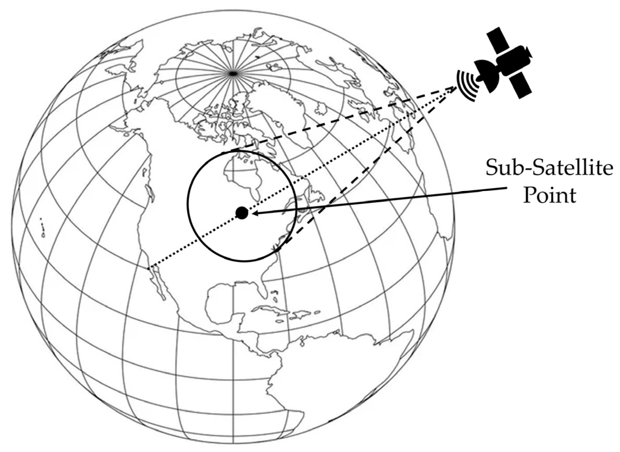
2.3. Calculation of the Satellite Position Dilution of Precision

The pseudo-range observation equation and the carrier phase observation equation for a single GNSS tracking station can be expressed as [26,27,28]
P r , j s = ρ i + c ( t r t s ) + T r s + I r , j s + ε r , j s ϕ r , j s = ρ i + c ( t r t s ) + λ j s N r , j s + T r s I r , j s + ξ r , j s ,
where ρ i is the geometric distance between satellite s and ground station r, t r and t s denote the clock delay of the station (receiver) and the visible satellite, respectively. T r s and I r , j s denote the tropospheric and ionospheric delays, respectively, while N r , j s is the integer phase ambiguity, c is the light celerity, and ε r , j s , ξ r , j s denote the pseudo-range and phase noises, respectively.
In observation Equation (6), the geometric distance between the i t h satellite ( X i , Y i , Z i ) and the ground station ( x , y , z ) is the Euclidean distance between them, which is expressed as
ρ i = ( X i x ) 2 + ( Y i y ) 2 + ( Z i z ) 2 .
After linearization, it can be expressed as
d ρ i = ( X i x ) d X i + ( Y i y ) d Y i + ( Z i z ) d Z i ( X i x ) 2 + ( Y i y ) 2 + ( Z i z ) 2 .
Similar to the DOP calculation, the coefficient matrix A of the observation equation for satellite i can be expressed as [18,25,26,29]
A = c x 1 i c y 1 i c z 1 i c x 2 i c y 2 i c z 3 i c x m i c y m i c z m i ,
where c x k i , c y k i , c z k i is the direction cosine from the ith satellite to the kth ground station for the total number of ground stations (m) that are visible to satellite i at a certain epoch.
Therefore, the cofactor matrix Q of observation matrix A can be expressed as
Q = ( A T A ) 1 = q 11 q 12 q 13 q 21 q 22 q 23 q 31 q 32 q 33 .
Finally, similar to the PDOP, the satellite position dilution of precision (SPDOP) value of satellite i at a certain epoch can be expressed as [18,29]
S P D O P = q 11 + q 22 + q 33 .

2.4. Intersatellite Links for SPDOP

ISLs are considered crucial for enhancing the accuracy of orbit determination and satellite clock estimation [30]. This is improved using a combination of GS observations and ISLs, which eventually enhance the precision of navigation without supplementary GS network augmentation [31,32,33]. In this study, ISLs are used to improve SPDOP, which is a criterion of the precision of orbit determination [18,29]. The specific observation model, when only the satellite position parameters are considered, is the geometric range between satellite i and satellite j , which can be expressed as
ρ i j = ( X i X j ) 2 + ( Y i Y j ) 2 + ( Z i Z j ) 2 ,
where ( X i , Y i , Z i ) and ( X j , Y j , Z j ) are the three-dimensional coordinates of satellite i and satellite j, respectively.
Using Equations (7) and (12), the coefficient matrix A I S L of the observation equation for satellite i with GSs observations and ISLs can be expressed as [29]
A I S L = c x 1 i c y 1 i c z 1 i c x 2 i c y 2 i c z 3 i c x m i c y m i c z m i c x ˜ 1 i c y ˜ 1 i c z ˜ 1 i c x ˜ n i c y ˜ n i c z ˜ n i ,
where c x k i , c y k i , c z k i is the direction cosine from the satellite i to the k t h ground station ( k = [ 1 , , m ] ), m is the total number of GSs that are visible to satellite i at a certain epoch, c x ˜ l i , c y ˜ l i , c z ˜ l i is the direction cosine from satellite i to satellite l ( l = [ 1 , , n ] ), and n is the total number of satellites that are visible along with the i t h satellite at a certain epoch. Therefore, the cofactor matrix Q I S L of the observation matrix A I S L can be expressed as
Q I S L = A I S L T A I S L 1 = q ˜ 11 q ˜ 12 q ˜ 13 q ˜ 21 q ˜ 22 q ˜ 23 q ˜ 31 q ˜ 32 q ˜ 33 .
Therefore, SPDOP with GS and ISL observations can be expressed as [18,29]:
S P D O P I S L = q ˜ 11 + q ˜ 22 + q ˜ 33 .

3. Methodology

Ground station deployment optimization (i.e., with respect to number and placement) is conducted based on an evolutionary algorithm. In this section, two cases of GS deployment are shown: global deployment optimization and regional deployment optimization. In each case, the objective and methodology are defined.

3.1. Objective and Methodology for Global Deployment

As satellite position is considered only for the observation model, at least 3 GSs should be visible to each satellite at any time. Therefore, it is necessary to achieve 3-HC. The objective is to maximize the observing rate and minimize the number of GSs. Another criterion is added as a sub-objective (third objective), which is the maximization of the distance between the two nearest GSs to avoid having a high density of GSs in the same area. Therefore, the objective fitness function becomes
C 1 = min k X k 1 = min k ( n G S k ) C ˜ 2 = min k _ H e a v y _ C o v e r a g e R N o n o b s c 3 = min 1 / min ( d i ) .
The coastline of the whole world, including continental land masses and ocean islands, in addition to Antarctica, was obtained from shapefiles (*.shp) from the National Oceanic and Atmospheric Administration (NOAA)’s [34] Global Self-consistent, Hierarchical, High-resolution Geography (GSHHG) database.
The method used for GS deployment in this study is based on the integration of three evolutionary algorithms, i.e., non-dominated sorting genetic algorithm-III (NSGA-III), strength Pareto evolutionary algorithm-II (SPEA-II) and multi-objective particle swarm optimization (MOPSO). A flow chart of this method and its detailed steps is shown in Figure A1 in Appendix A. Figure 3 shows the flow chart of the GS deployment optimization for global distribution.
The method used for GS deployment based on evolutionary algorithms is outlined below (Algorithm 1).
Algorithm 1. Optimal deployment method for global distribution of GSs
Step 0:Initialize the parameters: evolutionary algorithm parameters, number of populations N and maximum iteration (It).
Step 1:For a given k-heavy coverage of k = 3, generate N random integer values (according to the size of population), each in the interval n GS m i n ,   , n GS m a x .
Step 2:For each random integer m, generate m random coordinates, and check whether each set corresponds to land.
Step 3:For each population, evaluate the following objectives: the number of GSs and the observing rate according to the k-heavy coverage, in addition to the evaluation of the distance between the two nearest GSs in the population.
Step 4:Sort the population according to a non-dominated solution.
Step 5:Apply the main loop of the evolutionary algorithm (Appendix A) with all operations of crossover, mutation and selection.
Step 6:For each individual P in the population, check whether the value of the number of GSs (XP(1) refers to the variable of the number of GSs used as expressed in Equation (1) or whether it is changed (due to crossover and mutation operators) relative to the total number of GSs (|GS|). If the number of GSs (nGS) in a population has changed due to the crossover and mutation operations, generate a new deployment of GSs according to the new nGS (the same as for the generation of the initial populations).
Step 7:Due to crossover, mutation operations could change the variables; check the coordinates of GSs to see whether they correspond to land.
Step 8:Find the nearest land, and move the GSs here.
Step 9:Evaluate each individual population through the objective function.
Step 10:Check the number of iterations, and if iteration It <= Itmax (maximum iteration), go to Step 4; else, end of optimization.
In order to perform the optimization process of GS global deployment, the range of variables (i.e., the number of GSs and geographic coordinates) of each case is defined, as presented in Table 1.
The limits for the number of GSs are set according to the heavy observing coverage. In order to reach triple HC for ideal distribution (when oceans and seas are ignored), no less than 60 GSs are used. In addition, 150 is set as the upper limit for the number of GSs used based on several tests. Therefore, the lower and upper limits are fixed to 60 to 150, respectively.
For the longitude range, the limits are set for the whole range (from 180°W to 180°E), while the latitude limits are set from 85°S to 85°N due to the fact that the geographic grids (latitude, longitude) converge in the polar zones, and coverage can be ensured using only a few GSs (compared to the equatorial and near-equatorial zones).
The parameters of the hybrid method used in this optimization problem are shown in Table 2. It should be noted that the number of populations used is 300, and the number of generations is set to 30.
Based on the available guidelines of evolutionary algorithm handling, the parameters of the hybrid method of evolutionary algorithms are set. The mutation rate for NSGA-III should be no more than 0.1 and no less than 0.01, while the crossover and mutation rates are set to 0.8 and 0.2, respectively, in order to ensure the diversity of solutions (high crossover compared to mutation rate). A high value for the mutation rate means population instability, while a low value tends to decelerate evolution. For the MOPSO parameters, the recommended mutation rate is 0.1 if the population size is less than 500. The damping and inflation rates are set to 0.5 to avoid population dispersion and instability. Global and personal learning are set to 2 and 1, respectively, to ensure fast convergence of the algorithm, because low values could result in a premature solution. SPEA-II is a very stable algorithm according to the given solution, and the crossover and mutation parameters are both set to 0.5, while the archive number is set to one-third of the population (the maximum number of populations in the archive).

3.2. Objectives and Methodology for Regional Deployment

In the regional scheme of GS deployment, there is no way to reach any k-HC, which makes it difficult to determine an optimal configuration based only on the optimal SPDOP value.
Therefore, the number of GSs is fixed for algorithm simplification. In the case where the number of GSs is a variable for the optimization problem, the objective (SPDOP) of visible satellites in the regional area tends to be enhanced in proportion to the increase in the number of GSs. Moreover, there is an obvious concentration of GSs as long as SPDOP is evaluated only for visible satellites.
The number of GSs for global deployment is considered as a decision variable in order to obtain the minimum number needed to reach three-heavy observing coverage. Fixing the number of GSs in global deployment means an excessive number of scenarios need to be studied. For each fixed number of GSs, the optimal deployment must be found to reach the highest observing rate. Therefore, it is suitable to use the number of GSs as a decision variable for global deployment, unlike for regional cases, even though the algorithm complexity increases.
For the purpose of simplifying the optimization problem, the number of GSs is fixed for differing scenarios. The variables of this problem are the coordinates of the GSs.
X = [ λ 1 , φ 1 , , λ n G S , φ n G S ] ,
where λ i and φ i are the longitude and latitude of the ith ground station, respectively, and i = [ 1 , 2 , , n G S ] , where n G S is the number of GSs used for optimal deployment.
There is a single objective of optimization in these cases (only the mean SPDOP value). In addition, a sub-objective is added to ensure the good dispersion of GSs throughout the regional area to obtain a maximum number of observed satellites each time. This objective function is the maximization of the distance between the two nearest GSs (as the global distribution scheme). Therefore, the objective functions are expressed as
C = m e a n t O b s e r v a t i o m e a n P l a t , l o n g ( S P D O P S V i s i b l e _ S a t t , P c ˜ = min 1 / min d i ,
where t is the observing epoch (epoch of 1 min within 24 h of observation), P denotes the satellite’s position, S denotes all the visible satellites at epoch t, and d i is the distance between each station and the nearest GS in the same deployment (individual in the population).
The flow chart of the optimization method for GS regional deployment with the objective of SPDOP value minimization is shown in Figure 4. The principal step of the method used to determine the optimal deployment of GSs for local distribution is presented below (Algorithm 2).
Algorithm 2. Optimal deployment method for local distribution of GSs.
Step 0:Initialize the parameters of the algorithm and population size of N individuals.
Step 1:Define the number m of GSs that are used for optimal deployment.
Step 2:For each population, generate m random GSs in the selected regional area.
Step 3:Evaluate the objective function of each population (mean SPDOP) of visible satellites in addition to the sub-objective of the distance between the nearest GSs in the same population.
Step 4:Sort the population according to the ranking of min mean (SPDOP) and distance between GSs.
Step 5:Apply the main loop of evolutionary algorithms (Appendix A) with all operations of selection, crossover and mutation of individuals (or GSs).
Step 6:After each crossover and mutation operation, check whether the GS is in a regional area.
Step 7:If any ground station is outside the regional area, move it to the nearest regional land.
Step 8:Evaluate the objective function of each population (mean SPDOP) of visible satellites in addition to the sub-objective of the distance between the nearest GSs in the same population.
Step 9:Sort the population based on the ranking of the min mean (SPDOP) and the distance between GSs.
Step 10:Check the number of iterations (generation), and if it does not reach the max iterations go to Step 5; else, end the algorithm.
Both algorithms (i.e., for global or regional deployment) are similar when the number of GSs is fixed. When the number of GSs is considered as a decision variable, the number of variables of the optimization problem is no longer fixed and instead depends on the number of GSs used in each population. For each iteration, the number of variables changes from an individual solution to another due to the crossover and mutation operators of the evolutionary algorithm. These changes must be checked at each iteration in order to fit the value of the number of GSs used to the number of coordinates generated. If the number of GSs is considered as a variable in the regional deployment problem, the first algorithm (of global deployment) could be used.
Both algorithms are similar when the number of GSs used is fixed a priori. If not, the number of variables is also not fixed and, therefore, the main operators of the evolutionary algorithm become difficult to handle.

4. Results

Based on the methodology described in Section 3 and using the two versions of the algorithm, the results obtained for optimal GS deployment in the two schemes (global and regional) are shown and discussed in this section.

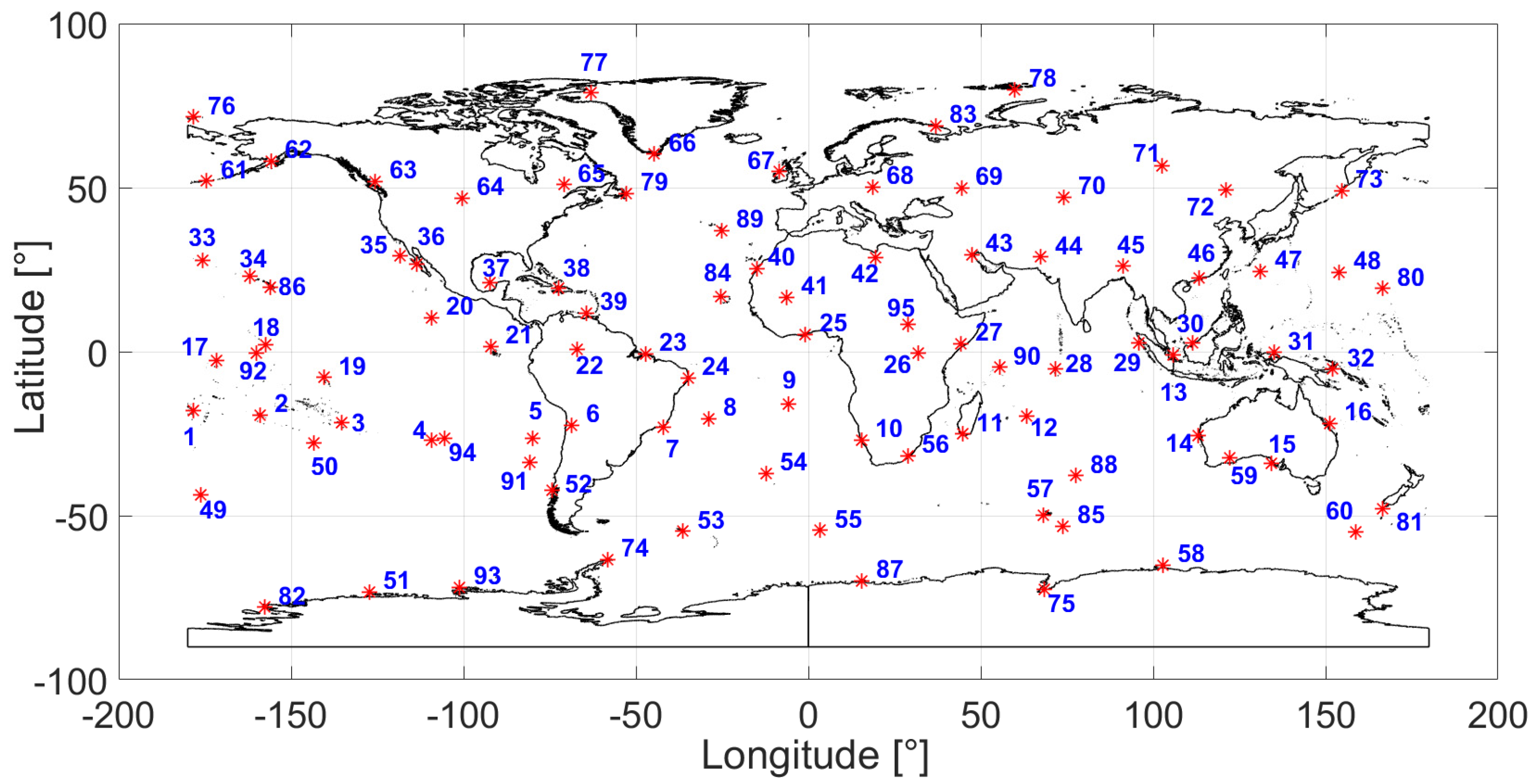
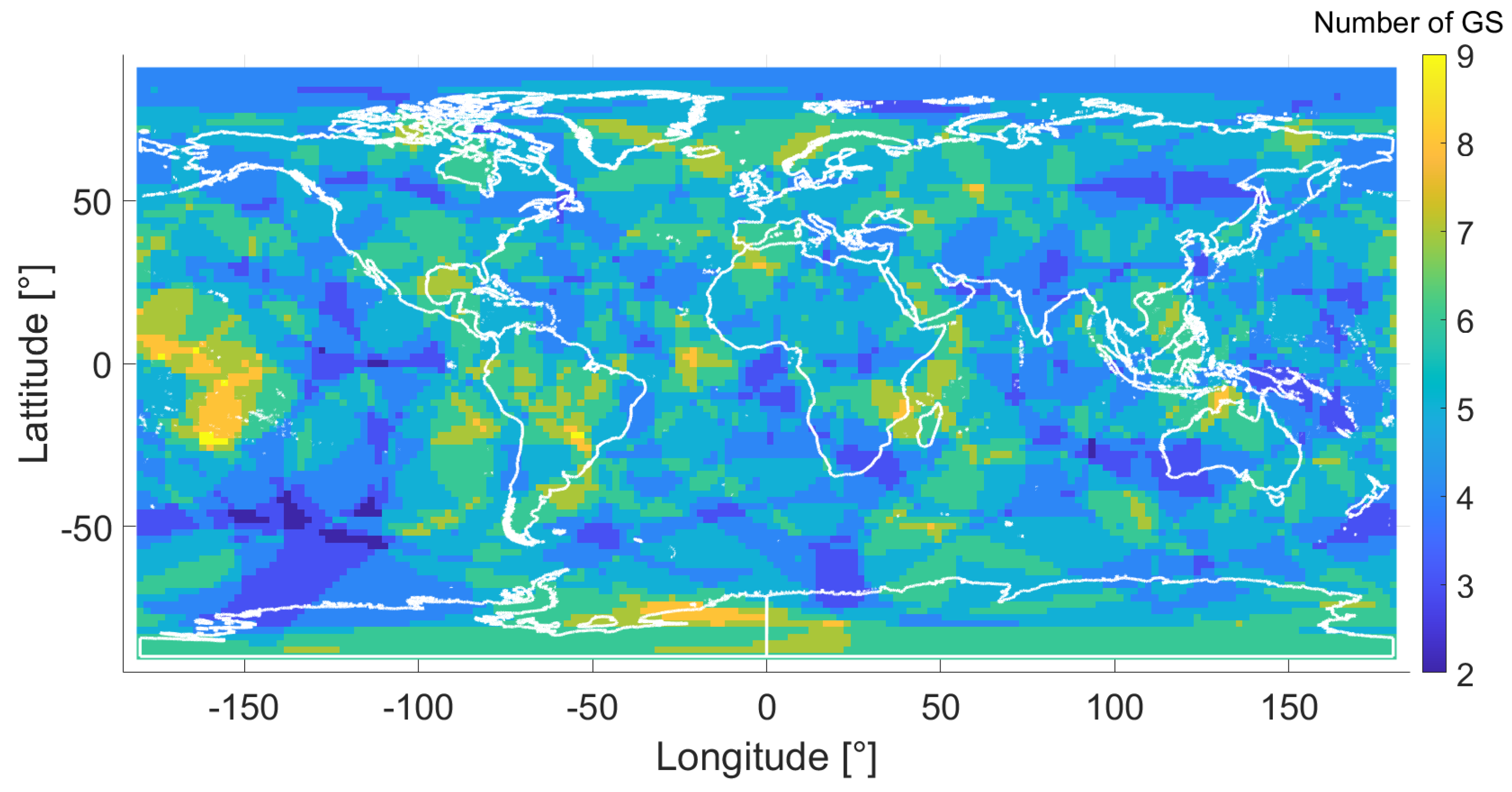
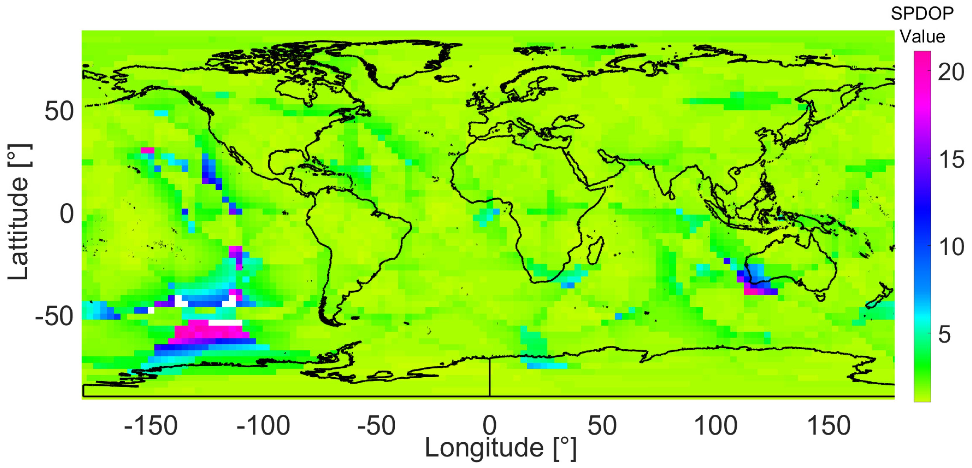
4.1. Global Deployment Optimization

Using the optimization of GSs (number and placement) with the method detailed in the previous section and shown in Figure 3, the solutions of three-heavy observing coverage to track the LEO constellation used in this study are shown in Figure 5.
The three best deployments with the highest 3-HC observing rates use 95, 138 and 148 GSs with observing rates of 97.37%, 97.97% and 97.98%, respectively. In view of the observing rates of each configuration, which are fairly close to each other, and according to the number of GSs used, the first configuration of 95 GSs is the best choice with a 97.37% observing rate, as shown in Figure 5.
The deployment of the optimal configuration of 95 GSs and a 97.37% observing coverage is shown in Figure 6.
In order to determine the performance of the GS deployment, a grid of 3° × 3° of the LEO flight area is created (the flight area of the LEO satellite is the 3D space that a satellite of a constellation could occupy at any epoch). The LEO flight area is formed as { l a t , l o n g , A l t } , where A l t is the orbit height, which is fixed for all the satellites ( A l t = 1176.6 km), and { l a t , l o n g } is the geographic coordinates. For each grid, the number of visible GSs per satellite corresponding to the grid position was checked.
The sub-satellite position is the point at which a line between the satellite and the center of the Earth intersects the Earth’s surface, and the location of this point is expressed in terms of latitude and longitude, as illustrated in Figure 7.
With the grid of the flight area of the LEO satellite (sub-satellite position), Figure 8 shows the observing coverage multiplicity, which is the number of GSs visible to the corresponding flight area position (latitude, longitude).
In the global deployment of 3-HC, the minimum number of GSs visible to each satellite each time over 5 degrees of elevation is two, and the maximum number of GSs is nine. Only in a few positions (2.63%), however, does the minimum number of GSs correspond to two. Otherwise, the minimum GSs visible per satellite is about 97.37%.
  • SPDOP Distribution
In order to determine the SPDOP distribution for this deployment, the flight area of the LEO satellites is used. The SPDOP value is calculated for each 3 × 3 grid and the altitude corresponding to the LEO orbit height { l a t , l o n g , A l t } . The distribution plot is projected as the sub-satellite position. The SPDOP distribution for 3-HC optimal distribution is shown in Figure 9.
The SPDOP value of the 3-HC deployment shows an even distribution compared to the 2-HC deployment, with a mean value of 1.86 and maximum value of 21.8. For some satellite positions, SPDOP is not determined because the number of GSs is less than three (the areas indicated in white), but this represents only 2.63% of the whole area. SPDOP is less than two for more than 82% of the satellite positions and is more than five for only 2.82%. In addition, the dispersion value is low where the standard deviation of SPDOP is equal to 1.045. Therefore, the SPDOP value shows uniform distribution for all satellite point positions, which means there is a uniform distribution of orbit determination for all LEO satellites in the constellation.
For global deployment, with 3-HC for the LEO constellation, SPDOP shows a good distribution with a mean value of 1.86. Therefore, it improves the accuracy of the orbit determination with 3-HC GS deployment for the LEO constellation. If only the satellite position in the observation model is considered for orbit determination, 3-HC may be suitable for achieving high precision.

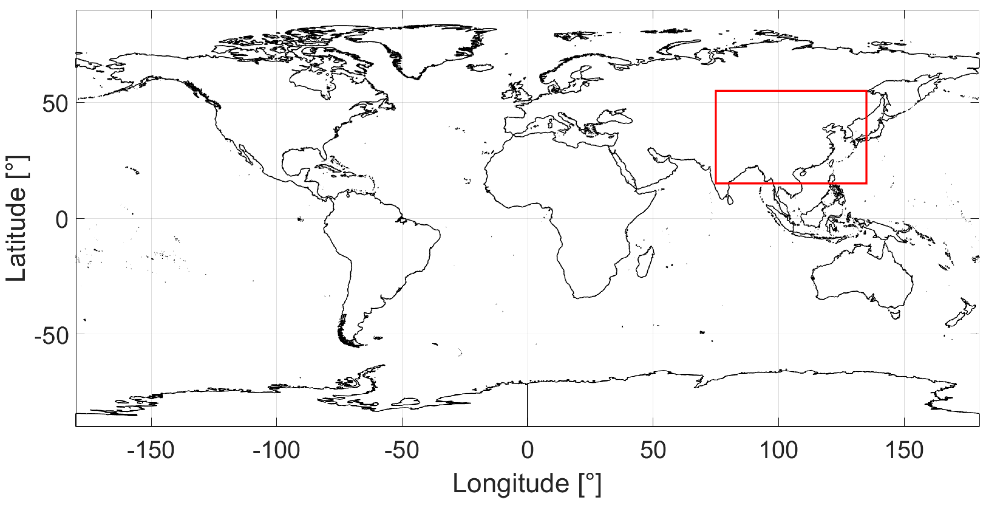
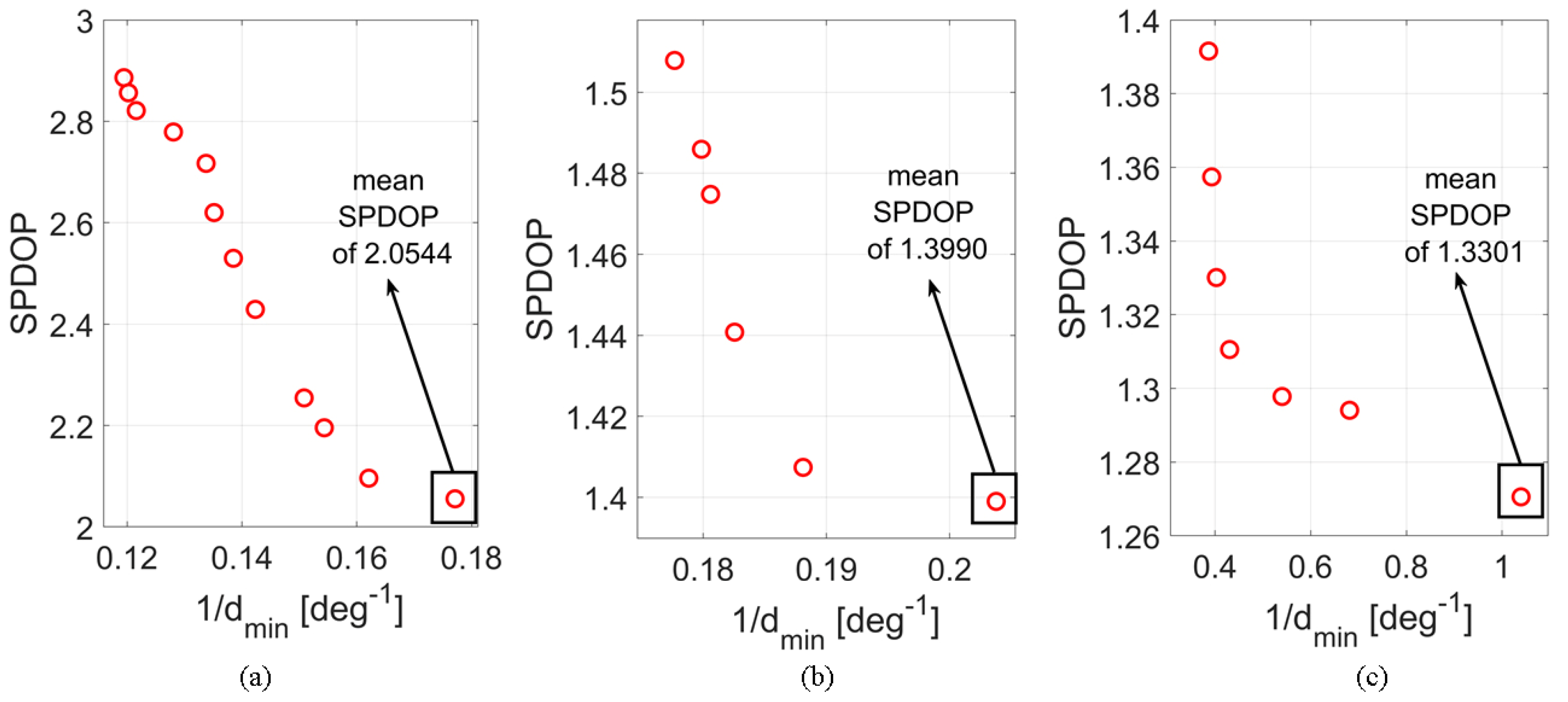
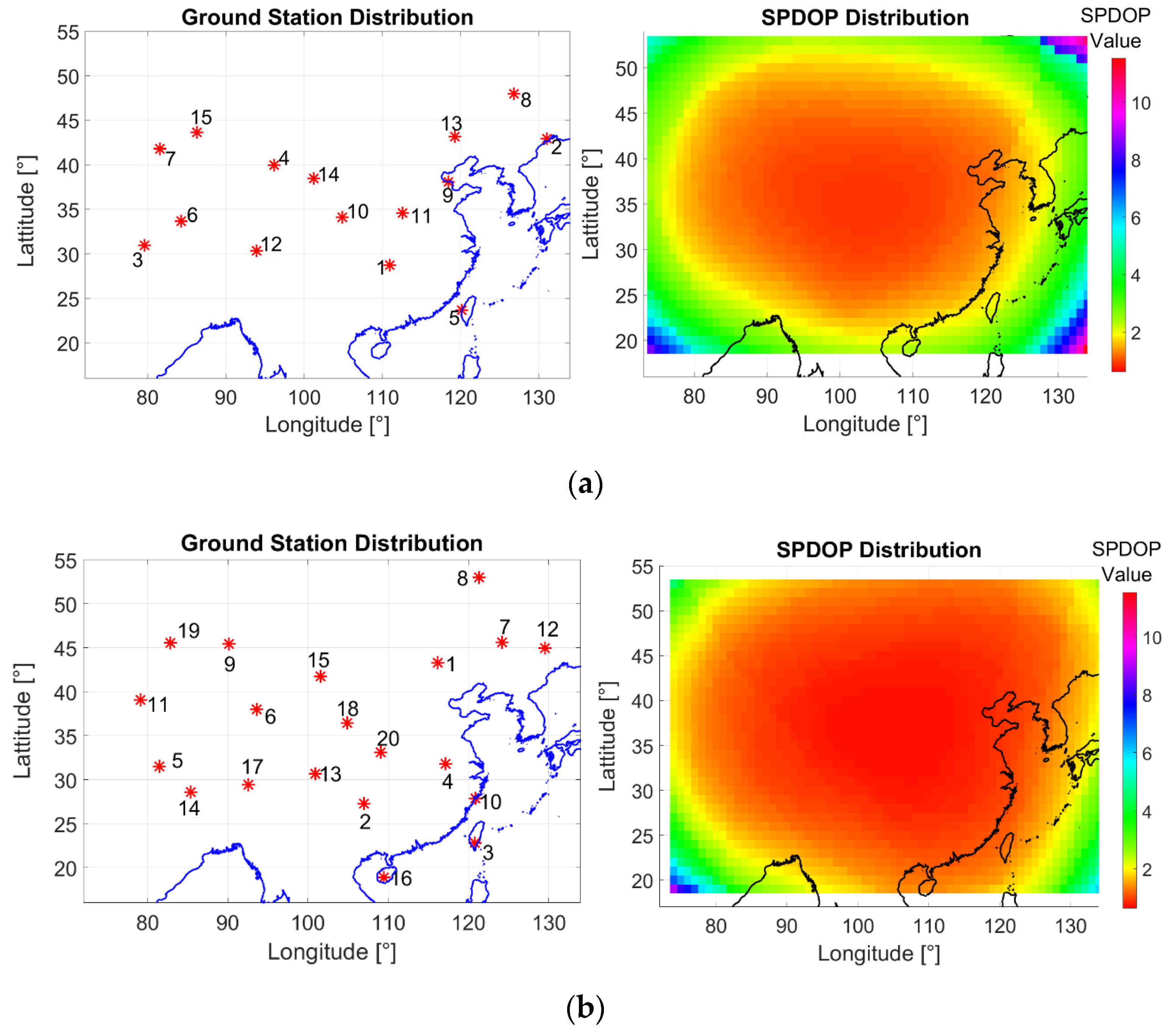
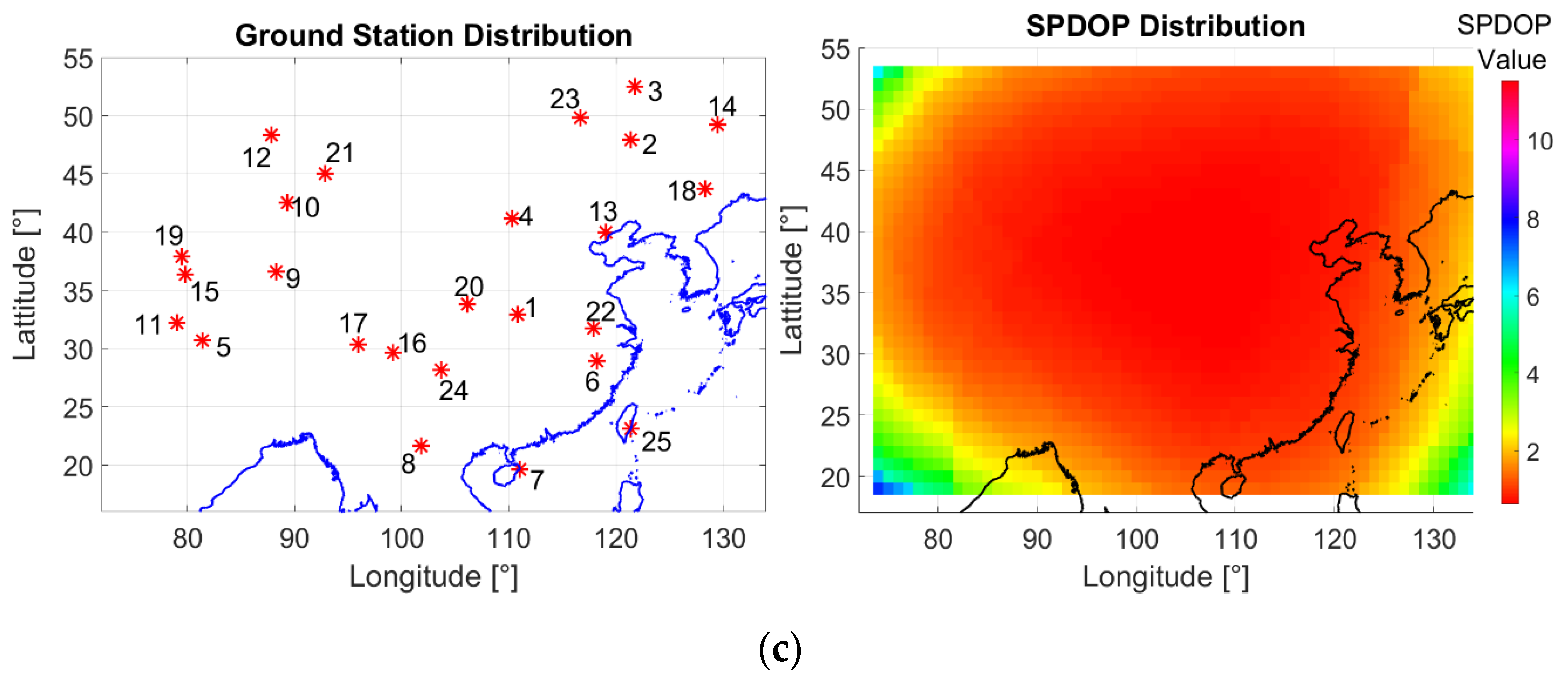
4.2. Regional Deployment Optimization

In the case of the regional distribution of GSs, the criterion for optimal deployment is the SPDOP. The SPDOP is an indicator used to evaluate the dilution of precision of satellite positions relative to GSs [23].
Using the method detailed for the three scenarios studied according to the number of GSs used, the optimization of regional deployment is performed. Remember that the objective of optimization is the minimization of the SPDOP, which is calculated only with the GSs.
The regional area used for the local deployment of GSs is shown in Figure 10, where it is delimited by a red rectangle. The regional area selected for GS deployment in the second scheme is Pacific East Asia. Table 3 shows the coordinates of this area.
The optimization process is performed using the method of regional deployment shown in Figure 4. The evolutionary algorithm parameters used in this optimization problem are shown in Table 2. The number of populations used is 150, and the number of generations (iterations) is set to 30.
According to the number of GSs used, three cases are simulated for the optimization of the regional distribution of GSs, as shown in Table 4, where the number of GSs is fixed at 15, 20 and 25.
Using the optimization method detailed in the previous sub-section, the optimization results of the two objectives (i.e., the SPDOP and the sub-objective of the maximization of the minimum distance between the two nearest GSs) are shown in Figure 11.
The solution shows, for each scenario (i.e., 15, 20 and 25 GSs), a Pareto front of the two objectives: the SPDOP and 1/dmin (refers to the inverse of the minimum distance between the two nearest GSs in the same deployment).
As the optimization is a two-objective problem with one objective and one sub-objective, the choice of the best solution is set according to the first objective (the minimum mean SPDOP). As the SPDOP is considered dominant in this optimization problem, only the solution with the minimum mean SPDOP value is considered as the final solution. Therefore, the optimal solutions for 15, 20 and 25 GSs present mean SPDOPs of 2.0544, 1.339 and 1.3301, respectively (See Figure 11). The optimal solutions correspond to minimum distances between the two nearest GSs in each deployment of 5.65°, 4.91° and 2.48°, respectively.
The optimal deployment of GSs for each scenario (15, 20 and 25 GSs) and the distribution of the SPDOP of the sub-satellite position for regional GS distribution are shown in Figure 12.
The increase in the number of GSs enhances the SPDOP value, which increases the precision of orbit determination. For the optimal deployment of 15 GSs, the mean SPDOP value is 2.0544. Using 20 GSs with optimal deployment, the mean SPDOP value is 1.3990. In the case of 25 GSs, the SPDOP is enhanced to a mean value of 1.3301. The performance results of the deployment for each scenario are shown in Table 5.
It is shown that the increase in the number of GSs in the same deployment creates a concentration of GSs in same area and even increases the SPDOP value.
The mean value of SPDOP decreases (enhancement in SPDOP distribution value) when the number of GSs increases. The SPDOP can reach 11.53 for the optimal deployment of 15 GSs, while the maximum value of the SPDOP is less than 7.6 for the deployment of 25 GSs. In the work of Zhang et al. [18], the mean SPDOP was determined for selected MEO BDS-2 satellites (C11, C12, C14) using two schemes with 30 GSs regionally and globally distributed. Table 6 shows the results of the mean SPDOP values and the corresponding standard deviations.
Compared to the SPDOP values of the MEO satellites, the mean SPDOP of the LEO constellation is better with global or regional GS distribution. In scheme 2, the SPDOP is around 208 with high dispersion (Std of 189.43), where 30 GSs are selected with global distribution, while it is around 1.86 with low dispersion (Std of 1.06) for LEO satellites. Therefore, precise orbit determination should be better for LEO satellites than MEO satellites.
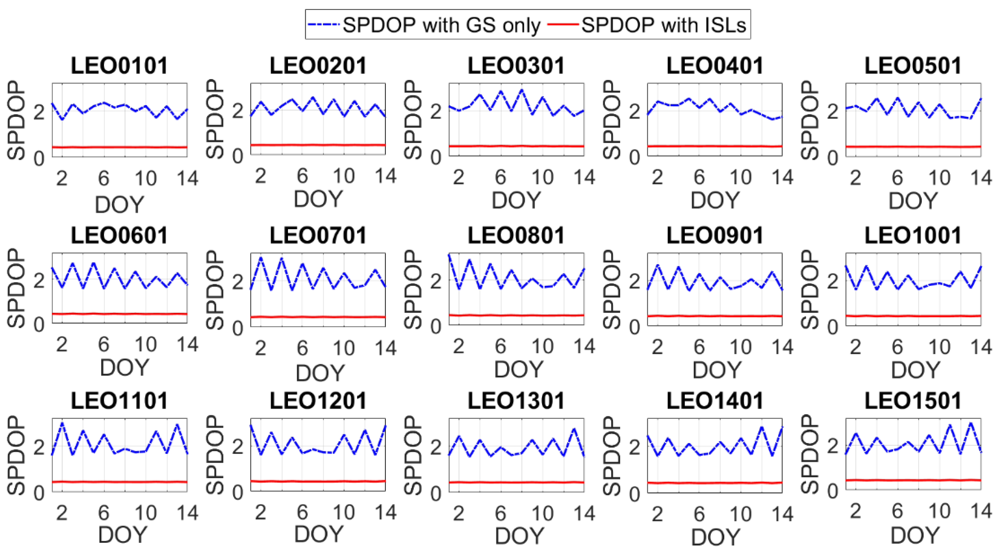
  • SPDOP with Ground Stations and Intersatellite Links
ISLs are used to enhance the accuracy of a satellite’s orbit. In this study, ISLs are evaluated for LEO SPDOP enhancements. LEO constellations are composed of a huge number of satellites compared to MEO (GNSS) constellations, which means the number of ISLs at each time is greater; therefore, the SPDOP value will be enhanced.
To evaluate the SPDOP of LEO satellites and due to the large number of satellites (210), the first satellite in each plane is selected (for example, LEO0301 denotes the first satellite (01) in the third (03) plane), in order to evaluate the SPDOP for 14 days of observation (DOY 1 to DOY 14 of the year of 2023). Figure 13 shows the SPDOP value of 15 LEO satellites with only GSs versus the SPDOP with GSs and ISLs (case of optimal 15 GSs). It should be noted that there is no weighting of observations; so, all the measurements are considered with equal weight.
SPDOP is improved using ISLs with visible GSs. It should be noted that the data visualization (of the mean SPDOP with 20 GSs and 25 GSs with ISLs) is not straightforward due to the similarity. For this reason, only the case of 15 GSs is shown. For the 15 LEO satellites considered in this evaluation of 14 days of observation, the mean SPDOP improved from 2.058 to 0.439, from 1.403 to 0.422, and from 1.33 to 0.409 for 15, 20 and 25 GSs, respectively. Using ISLs, SPDOP is enhanced and tends to reduce the dispersion between the three deployment scenarios of 15, 20 and 25 GSs.
The results of the SPDOP—mean, maximum and minimum values—for each deployment with 14 days of observation are shown in Table 7. The SPDOP value is dependent on the number of ISLs in each epoch. The LEO constellation, with a large number of ISLs, has an advantage in enhancing the precision of orbit determination when SPDOP is enhanced due to the large number of ISLs observed at each epoch.
As is shown in Table 8, the number of ISLs at each epoch (1 min) is at least 37, while it can reach a maximum of 69. In 14 days of observation, the average number of ISLs observed at each epoch (1 min) is around 51.43 for each LEO satellite.

5. Discussion

5.1. Global Deployment Optimization

In many areas of the 3-HC deployment (see Figure 8), the coverage multiplicity is equal to nine, which means nine GSs are visible to the satellite at the same time, when it is positioned in the corresponding area. The concentration of GSs in these areas is due to moving the GSs which were not on land, particularly those in oceans. The positions of the GSs are optimized according to the maximum coverage. However, where they are not applicable due to being in oceans and seas, the GSs must be moved to the nearest land. As seen in Figure 6, there is an obvious concentration of GSs in the Pacific region, the part of the Earth most occupied by seas. This concentration creates a high level of coverage multiplicity compared to other regions. Table 9 shows the observing rate of 3-HC deployment with simple, double, triple and quadruple coverage. In the optimal deployment of 3-HC, the best obtained observing rate is 97.37%, which means that all satellites at any epoch are visible by at least two GSs, while 97.37% of the observing duration (24 h) means each satellite is visible by at least three GSs.
For this deployment, quadruple-heavy observing coverage (4-HC) was achieved 92.01% of the time. Hence, within 92.01% of the observing duration, each satellite is visible by at least four GSs. With threefold coverage of GSs for each satellite at each epoch, the SPDOP value could be determined if only the satellite position was considered for the observation equation.

5.2. Regional Deployment Optimization

In view of the fact that precise orbit information is required for LEO constellation navigation, the global deployment of GSs offers a good opportunity for highly accurate orbit determination. When LEO satellites are visible to at least three GSs at a given time, the period without GS network observation tends toward 0. Therefore, at each epoch time, all satellite orbits can be determined with high precision.
In regional deployment and according to the LEO satellite’s revisit time (around 2 h), the period of GS coverage is around 10 min. In addition, the average observed period of each satellite increases in proportion to the width of the regional area. However, the previous results for global GS deployment suggest that even if all land is considered for deployment, having a high level of heavy observing coverage is limited by the available land on Earth. As more than 71% of the globe is oceans and seas, further study and analysis are required to determine the possibility of deployment in Antarctica and isolated island areas. This study is based on the supposition that any part of Earth—whether land, ocean or island—can be considered for GS deployment. Hence, the scenario of the regional distribution of GSs persists as a solution in cases where global distribution fails due to different causes.
The SPDOP value of LEO satellites was evaluated based on a comparison between LEO, MEO, IGSO and GEO satellites. Selected satellites of the BDS constellation were evaluated using SPDOP values in the work of Zhang et al. [29]. Table 10 shows the mean SPDOP value for GSs only and for GSs and ISLs (in one-way ranging). The selected satellites in the mentioned study were in the GEO, IGSO and MEO constellations. It should be noted that the values in the table are the mean value and mean Std of SPDOP, according to Zhang et al. [29].
It can be seen that SPDOP presents a low value for the LEO satellite compared to other satellites. The mean SPDOP value of the LEO is no more than 2.06 with 15 regionally distributed GSs (without ISLs in one-way ranging), while it exceeds 185, 354 and 475 for the MEO, IGSO and GEO satellites, respectively. In addition to excellent SPDOP distribution, the dispersion values of these satellites are obvious compared to LEO due to the large change in geometry. The strong impact of ISLs (used in one-way ranging) is obvious in their enhancement of SPDOP values.
In the observation based on ISLs and GSs, the mean SPDOP is improved from 475.72 to 12.00, from 354.27 to 2.12, and from 185.10 to 148.65 for the GEO, IGSO and MEO satellites, respectively (according to [29]). For LEO satellites, and using ISLs in addition to GSs in observation, the SPDOP value improves significantly, reaching 0.44 due to the large number of ISL observations available in each epoch time.
Compared to MEO and high Earth orbit (GEO and IGSO), the LEO satellite constellation presents an excellent SPDOP, which indicates a high precision of orbit determination.

6. Conclusions

In this study, two schemes of GS deployment for the tracking of LEO constellations are presented, namely global deployment and regional deployment.
Firstly, for global deployment, GS number and placement are optimized based on evolutionary algorithms. For triple-heavy observing coverage (3-HC), the optimization process includes two objectives (i.e., the observing rate and the number of GSs used for deployment) in addition to another sub-objective (the minimum distance between the two nearest GSs) in order to avoid the concentration of GSs in the same place. Subsequently, 95 ground stations formed the optimal deployment to reach 3-HC. The 95 GSs for 3-HC reached a 97.63% observing rate and 92.01% was obtained for quadruple coverage. The distribution of SPDOP, when only the GSs are considered, is discussed.
Secondly, for regional deployment and using three scenarios according to the number of GSs used, SPDOP decreases with the increasing number of GSs. A regional area in East Asia is chosen as the local area for deployment under three scenarios with 15, 20 and 25 ground stations used. The optimal SPDOP values are 2.05, 1.40 and 1.33, respectively. The results were enhanced with ISLs, where the SPDOP mean value was reduced from 2.06 to 0.44 for 15 GSs, from 1.40 to 0.42 for 20 GSs, and from 1.33 to 0.41 for 25 GSs.
The complexity of GS deployment for LEO satellite constellations is due to the majority of the globe being occupied by oceans and seas. The choice of the best method to determine the optimal deployment in addressing this problem is not clear. As seen from the results obtained in this study, evolutionary algorithms present a suitable solution. These algorithms can be applied to solve real problems in the field of navigation with LEO satellites. In terms of future work, it is recommended that the developed algorithm be reused for other scenarios such as 4-heavy observing coverage or for regional deployment in other regions, even without a fixed number of GSs.
Furthermore, the hybrid method of the evolutionary algorithms used presents the advantage of fast convergence compared to other evolutionary algorithms such as NSGA, MOSPO and SPEA, when each is used in isolation. Each evolutionary algorithm (such as NSGA, MOSPO, etc.) could be used instead of the hybrid method, but convergence may take too long. The hybrid method is used due to its fast convergence, as many tests have confirmed.

Author Contributions

Conceptualization, M.K. and F.W.; methodology, M.K.; software, M.K. and A.O.; validation, A.T. and X.S.; investigation, M.K., F.W. and A.O.; writing—original draft preparation, M.K.; writing—review and editing, F.W. and A.T.; visualization, A.O.; supervision, F.W.; funding acquisition, F.W. All authors have read and agreed to the published version of the manuscript.

Funding

This research received no external funding. The APC was funded by Beihang University.

Data Availability Statement

Data are contained within the article.

Acknowledgments

We are very grateful for the contributions and comments of peer reviewers.

Conflicts of Interest

The authors declare no conflicts of interest.

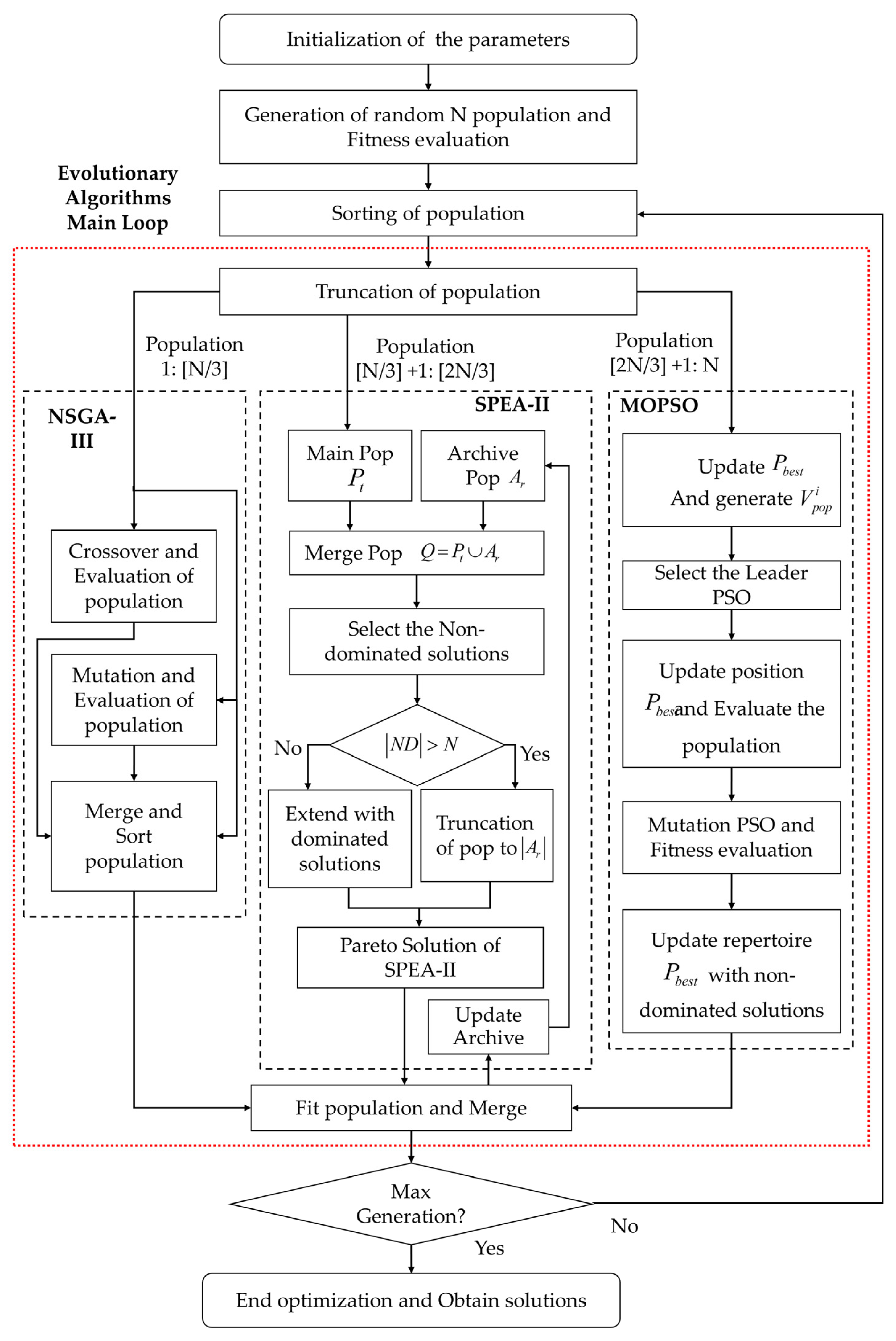
Appendix A. Hybrid Method with Integration of Non-Dominated Sorting Genetic Algorithm-III (NSGA-III), Strength Pareto Evolutionary Algorithm-II (SPEA-II), and Multi-Objective Particle Swarm Optimization (MOPSO)

Figure A1 shows the flow chart for the hybrid method of the evolutionary algorithms (HMEAs) used for ground station deployment. It should be noted that for this method based on NSGA-III [35], SPEA-II [36] and MOPSO [37], the codes are available online in the public file exchange of MathWorks.
A 2: Overall procedure of the hybrid method of evolutionary algorithms (HMEAs).
The overall procedure is outlined as follows:
Algorithm A1. Overall procedure of the hybrid method of evolutionary algorithms (HMEAs).
Step 0Initialize the parameters of each algorithm NSGA-III, SPEA-II and MOPSO.
Step 1Generate a random population of N individuals, and evaluate the fitness.
Step 2Sort the population according to the ranking based on non-dominated solutions.
Step 3Truncate the population into three sub-populations of [N/3] individuals for each.
Step 4Fit each sub-population to the individual structure of the used algorithm, because the initialization used the NSGA-III individual structure.
Submit each sub-population for processing to each algorithm: the first with NSGA-III, the second with SPEA-II and the last with MOPSO.
Step 5After each sub-population is processed in the corresponding population, fit to the NSGA-III individual structure and merge all sub-populations of [N/3] to the whole solution of N individuals.
Step 6Update the new archive with the truncation of the merged population after sorting according to the raw fitness of SPEA-II.
Step 7Check the number of generations it; if it > MaxIt? end optimization;
else, it = it + 1, and go to Step 2.
Figure A1. Flow chart of the hybrid method of evolutionary algorithms.
Remotesensing 16 00810 g0a1
In the NGSA-III process:
  • Apply the operator of the crossover to a random number of crossover individuals N C r o s s o v e r , which is calculated by the probability of crossover P C r o s s o v e r of the NSGA-III parameter as N C r o s s o v e r = 0.5 * [ 2 P C r o s s o v e r . N p o p / 3 ] .
  • Apply the operator of the mutation to a random number of mutated individuals N M u t a t e s , which is calculated by the probability of mutation P M u t a t i o n of the NSGA-III parameters as N M u t a t i o n s = [ P M u t a t i o n . N p o p / 3 ] .
  • Merge the main population and individuals that have undergone crossover and mutation to select the next new population by sorting based on ND solutions.
In the SPEA-II process:
  • Merge the main population and archive population, and after fitness evaluation, select the ND solutions based on the strength and raw operator.
  • According to the number of individuals in ND solutions, extend the ND solutions by the dominant solution if the number of ND solutions is less than the archive size, or truncate the ND solutions if the size exceeds the archive size.
  • The new population is the solution improved by SPEA-II, while the new archive is updated after merging all sub-populations.
In the MOPSO process:
  • Update the best population and generate the velocity for each particle (individual), and the repertory is updated according to the non-dominated sorting solution of the sub-population.
  • For each individual, select a leader from the repertory, and that particle should move toward its leader.
  • Update the particle velocity after the selection of a leader; therefore, update the position and evaluate the individuals in the population.
  • Apply the mutation according to the number of mutates for the MOPSO mutation parameter and evaluate the mutated individuals.
After the sorting and selection of the ND solution, the repertory will be updated with the ND solution, considered as the improved solution by MOPSO.

References

  1. Joerger, M.; Gratton, L.; Pervan, B.; Cohen, C.E. Analysis of Iridium-augmented GPS for floating carrier phase positioning. Navigation 2010, 57, 137–160. [Google Scholar] [CrossRef]
  2. Tan, Z.; Qin, H.; Cong, L.; Zhao, C. New method for positioning using IRIDIUM satellite signals of opportunity. IEEE Access 2019, 7, 83412–83423. [Google Scholar] [CrossRef]
  3. Ke, M.; Lv, J.; Chang, J.; Dai, W.; Tong, K.; Zhu, M. Integrating GPS and LEO to accelerate convergence time of precise point positioning. In Proceedings of the 2015 International Conference on Wireless Communications & Signal Processing (WCSP), Nanjing, China, 15–17 October 2015; pp. 1–5. [Google Scholar]
  4. Li, X.; Ma, F.; Li, X.; Lv, H.; Bian, L.; Jiang, Z.; Zhang, X. LEO constellation-augmented multi-GNSS for rapid PPP convergence. J. Geod. 2019, 93, 749–764. [Google Scholar] [CrossRef]
  5. Ge, H.; Li, B.; Nie, L.; Ge, M.; Schuh, H. LEO constellation optimization for LEO enhanced global navigation satellite system (LeGNSS). Adv. Space Res. 2020, 66, 520–532. [Google Scholar] [CrossRef]
  6. Li, M.; Xu, T.; Guan, M.; Gao, F.; Jiang, N. LEO-constellation-augmented multi-GNSS real-time PPP for rapid re-convergence in harsh environments. GPS Solut. 2021, 26, 29. [Google Scholar] [CrossRef]
  7. Nie, X.; Li, M.; Ma, F.; Wang, L.; Zhang, X. LEO Constellation Design Based on Dual Objective Optimization and Study on PPP Performance. In China Satellite Navigation Conference (CSNC 2021) 2021 Proceedings; Yang, C., Xie, J., Eds.; Lecture Notes in Electrical Engineering; Springer: Singapore, 2021; Volume 773, pp. 197–207. [Google Scholar]
  8. Zhang, Y.; Li, Z.; Li, R.; Wang, Z.; Yuan, H.; Song, J. Orbital design of LEO navigation constellations and assessment of their augmentation to BDS. Adv. Space Res. 2020, 66, 1911–1923. [Google Scholar] [CrossRef]
  9. Han, Y.; Wang, L.; Fu, W.; Zhou, H.; Li, T.; Xu, B.; Chen, R. LEO navigation augmentation constellation design with the multi-objective optimization approaches. Chin. J. Aeronaut. 2021, 34, 265–278. [Google Scholar] [CrossRef]
  10. Yang, M.; Dong, X.; Hu, M. Design and simulation for hybrid LEO communication and navigation constellation. In Proceedings of the 2016 IEEE Chinese Guidance, Navigation and Control Conference (CGNCC), Nanjing, China, 12–14 August 2016; pp. 1665–1669. [Google Scholar]
  11. He, X.; Hugentobler, U. Design of Mega-Constellations of LEO Satellites for Positioning. In China Satellite Navigation Conference (CSNC 2018) 2018 Proceedings; Sun, J., Yang, C., Guo, S., Eds.; Lecture Notes in Electrical Engineering; Springer: Singapore, 2018; Volume 497, pp. 663–673. [Google Scholar]
  12. Guan, M.; Xu, T.; Gao, F.; Nie, W.; Yang, H. Optimal walker constellation design of LEO-based global navigation and augmentation system. Remote Sens. 2020, 12, 1845. [Google Scholar] [CrossRef]
  13. Dvorkin, V.; Karutin, S. Optimization of the global network of tracking stations to provide GLONASS users with precision navigation and timing service. Gyroscopy Navig. 2013, 4, 181–187. [Google Scholar] [CrossRef]
  14. Li, H.; Li, Y.; Dai, T.; Wang, L.; Wang, J. Real-time GPS satellite clock offset determination based on the TIN global station-selecting method. J. Geomat. Sci. Technol. 2017, 34, 441–444. [Google Scholar]
  15. Zhang, R.; Yang, Y.; Zhang, Q.; Huang, G.; Wang, L.; Qu, W.; Zhao, H. Optimal Estimation of Dynamic Parameters of BDS Orbit for Optimal Selection of Tracking Stations. J. Geod. Geodyn. 2016, 36, 216–220. [Google Scholar] [CrossRef]
  16. Shah Sadman, A.A.M.; Hossam-E-Haider, M. Study of GNSS Parameters and Environmental Factors over Bangladesh Intended for Selecting Ideal Ground Station Location for SBAS. In Proceedings of the 2021 2nd Global Conference for Advancement in Technology (GCAT), Bangalore, India, 1–3 October 2021; pp. 1–6. [Google Scholar]
  17. Yang, X.; Wang, Q.; Xue, S. Random optimization algorithm on GNSS monitoring stations selection for ultra-rapid orbit determination and real-time satellite clock offset estimation. Math. Probl. Eng. 2019, 2019, 7579185. [Google Scholar] [CrossRef]
  18. Zhang, R.; Zhang, Q.; Huang, G.; Wang, L.; Qu, W. Impact of tracking station distribution structure on BeiDou satellite orbit determination. Adv. Space Res. 2015, 56, 2177–2187. [Google Scholar] [CrossRef]
  19. Zhang, R.; Tu, R.; Zhang, P.; Fan, L.; Han, J.; Wang, S.; Hong, J.; Lu, X. Optimization of ground tracking stations for BDS-3 satellite orbit determination. Adv. Space Res. 2021, 68, 4069–4087. [Google Scholar] [CrossRef]
  20. Zhang, R.; Tu, R.; Zhang, P.; Fan, L.; Han, J.; Lu, X. Orbit determination of BDS-3 satellite based on regional ground tracking station and inter-satellite link observations. Adv. Space Res. 2021, 67, 4011–4024. [Google Scholar] [CrossRef]
  21. Liu, X.; Ge, Y.; Zhao, C.; Li, B.; Zhou, R. A Study on Global Monitoring Station Optimization Deployment Method Based on Navigation Satellite Quadruple Observing Coverage. In Proceedings of the 2021 International Conference on Communications, Information System and Computer Engineering (CISCE), Beijing, China, 14–16 May 2021; pp. 394–399. [Google Scholar]
  22. Kopacz, J.; Roney, J.; Herschitz, R. Optimized ground station placement for a mega constellation using a genetic algorithm. In Proceedings of the 33rd Annual AIAA/USU Conference on Small Satellites, Logan, UT, USA, 3–8 August 2019; p. SSC19-WP11-05. [Google Scholar]
  23. Carlton-Wippern, K.C. Satellite Position Dilution of Precision (SPDOP). In Proceedings of the 1997 AAS/AIAA Astrodynamics Specialist Conference, Sun Valley, ID, USA, 4–7 August 1997; pp. 133–146. [Google Scholar]
  24. Montenbruck, O.; Steigenberger, P.; Prange, L.; Deng, Z.; Zhao, Q.; Perosanz, F.; Romero, I.; Noll, C.; Stürze, A.; Weber, G.; et al. The Multi-GNSS Experiment (MGEX) of the International GNSS Service (IGS)—Achievements, prospects and challenges. Adv. Space Res. 2017, 59, 1671–1697. [Google Scholar] [CrossRef]
  25. Ge, H.; Li, B.; Ge, M.; Shen, Y.; Schuh, H. Improving BeiDou precise orbit determination using observations of onboard MEO satellite receivers. J. Geod. 2017, 91, 1447–1460. [Google Scholar] [CrossRef]
  26. Wu, F.; Kubo, N.; Yasuda, A. Performance Evaluation of GPS Augmentation Using Quasi-Zenith Satellite System. IEEE Trans. Aerosp. Electron. Syst. 2004, 40, 1249–1261. [Google Scholar] [CrossRef]
  27. Ge, M.; Gendt, G.; Rothacher, M.; Shi, C.; Liu, J. Resolution of GPS carrier-phase ambiguities in precise point positioning (PPP) with daily observations. J. Geod. 2008, 82, 389–399. [Google Scholar] [CrossRef]
  28. Kouba, J.; Héroux, P. Precise point positioning using IGS orbit and clock products. GPS Solut. 2001, 5, 12–28. [Google Scholar] [CrossRef]
  29. Zhang, R.; Tu, R.; Fan, L.; Zhang, P.; Liu, J.; Han, J.; Lu, X. Contribution analysis of inter-satellite ranging observation to BDS-2 satellite orbit determination based on regional tracking stations. Acta Astronaut. 2019, 164, 297–310. [Google Scholar] [CrossRef]
  30. Kur, T.; Liwosz, T.; Kalarus, M. The application of inter-satellite links connectivity schemes in various satellite navigation systems for orbit and clock corrections determination: Simulation study. Acta Geod. Geophys. 2021, 56, 1–28. [Google Scholar] [CrossRef]
  31. Yang, Y.; Yang, Y.; Hu, X.; Chen, J.; Guo, R.; Tang, C.; Zhou, S.; Zhao, L.; Xu, J. Inter-satellite link enhanced orbit determination for BeiDou-3. J. Navig. 2020, 73, 115–130. [Google Scholar] [CrossRef]
  32. Xie, X.; Geng, T.; Zhao, Q.; Cai, H.; Zhang, F.; Wang, X.; Meng, Y. Precise orbit determination for BDS-3 satellites using satellite-ground and inter-satellite link observations. GPS Solut. 2019, 23, 40. [Google Scholar] [CrossRef]
  33. He, X.; Hugentobler, U.; Schlicht, A.; Nie, Y.; Duan, B. Precise orbit determination for a large LEO constellation with inter-satellite links and the measurements from different ground networks: A simulation study. Satell. Navig. 2022, 3, 22. [Google Scholar] [CrossRef]
  34. NOAA. National Oceanic and Atmospheric Administration. Available online: www.ngdc.noaa.gov (accessed on 10 August 2023).
  35. Heris, M.K. NSGA-III: Non-dominated Sorting Genetic Algorithm, the Third Version—MATLAB Implementation. Yarpiz. 2016. Available online: https://yarpiz.com/456/ypea126-nsga3 (accessed on 15 April 2023).
  36. Mostapha, K.H. Strength Pareto Evolutionary Algorithm 2 (SPEA2). Available online: https://www.mathworks.com/matlabcentral/fileexchange/52871-strength-pareto-evolutionary-algorithm-2-spea2 (accessed on 20 September 2023).
  37. Víctor, M.-C. Multi-Objective Particle Swarm Optimization (MOPSO). Available online: https://www.mathworks.com/matlabcentral/fileexchange/62074-multi-objective-particle-swarm-optimization-mopso (accessed on 11 August 2023).
Figure 1. LEO satellite constellation of Walker star pattern 87.3°: 210/15/6.
Remotesensing 16 00810 g001
Figure 2. Variable (chromosome) structure.
Remotesensing 16 00810 g002
Figure 3. Flow chart of the optimization method for the global deployment of GSs.
Remotesensing 16 00810 g003
Figure 4. Flow chart of the optimization method for GS regional deployment.
Remotesensing 16 00810 g004
Figure 5. Solution of objective optimization for 3-heavy observing coverage deployment. The parameter nGS refers to the number of GSs used in deployment, while Robs refers to the observing rate to reach 3-HC for this deployment.
Remotesensing 16 00810 g005
Figure 6. GSs distribution for tracking the LEO constellation with 3-HC.
Remotesensing 16 00810 g006
Figure 7. Sub-satellite position point.
Remotesensing 16 00810 g007
Figure 8. Observing coverage multiplicity of GSs for 3-HC.
Remotesensing 16 00810 g008
Figure 9. Satellite position dilution of precision distribution (SPDOP) of 3-HC deployment.
Remotesensing 16 00810 g009
Figure 10. Location of the selected area for regional GS deployment.
Remotesensing 16 00810 g010
Figure 11. Pareto front solution of regional GS deployment optimization: (a) 15 GSs, (b) 20 GSs and (c) 25 GSs. The term 1/dmin refers to the inverse of the minimum distance (expressed in degree units) between the two nearest GSs in the same deployment.
Remotesensing 16 00810 g011
Figure 12. GS distribution and SPDOP of the sub-satellite position for the LEO satellite constellation: (a) 15 GSs, (b) 20 GSs and (c) 25 GSs.
Remotesensing 16 00810 g012aRemotesensing 16 00810 g012b
Figure 13. The mean SPDOP of 15 LEO satellites with optimal deployment for 14 days of observation of 15 GSs with ISLs.
Remotesensing 16 00810 g013
Table 1. Range of variables for the optimization of GS deployment.
VariablesMin Number
of GSs ( n GS min )
Max Number
of GSs ( n GS max )
Longitudes
[°]
Latitudes
[°]
Value60150180W~180E85S~85N
Table 2. Algorithm parameters of the hybrid method for GS deployment optimization.
AlgorithmParameterValue
Non-dominated sorting genetic algorithm-III
(NSGA-III)
Crossover probability0.8
Mutation probability0.2
Mutation rate0.05
Multi-objective particle swarm optimization
(MOPSO)
Inertia weight0.4
Damping rate0.5
Inflation rate0.5
Mutation rate0.1
Personal learning1
Global learning2
Strength Pareto evolutionary algorithm-II
(SPEA-II)
Crossover probability0.5
Mutation probability0.5
Number archive to population ratio1/3
Table 3. Geographic limits of the selected area.
CoordinatesLongitude [°]Latitude [°]
Value75E~135E17N~55N
Table 4. Number of GSs used for regional deployment.
Scenario Case123
Number of GSs used152025
Table 5. SPDOP statistics for optimal deployment.
Scenario Mean SPDOPMax SPDOPStd of SPDOP
15 GSs2.054411.52660.7973
20 GSs1.39909.00000.4701
25 GSs1.33017.56960.4687
Table 6. Statistics of SPDOP of MEO satellites [18].
SchemeMean SPDOPStd SPDOPObservation
Scheme 1207.97189.4330 GSs (focus on Eastern hemisphere)
Scheme 2149.43126.1730 GSs (globally distributed)
Table 7. SPDOP statistics for 14 days of observation.
DeploymentParametersMean SPDOPMax SPDOPMin SPDOP
15 GSsGSs only2.0583.1431.516
GSs and ISLs0.4390.4530.435
20 GSsGSs only1.4032.0631.077
GSs and ISLs0.4220.4370.409
25 GSsGSs only1.3301.9451.011
GSs and ISLs0.4090.4250.396
Table 8. Number of intersatellite links (ISLs) for each epoch for 14 days of observation.
ParametersMaxMinMeanStd
Value643751.438.68
Table 9. Observation rate for the GS deployment of 3-heavy observing coverage (HC).
ParameterSingle-Heavy Observing Coverage 1-HCDouble-Heavy Observing Coverage 2-HCTriple-Heavy Observing Coverage 3-HCQuadruple-Heavy Observing Coverage 4-HC
Value100%100%97.37%92.01%
Table 10. SPDOP value comparison without and with ISLs.
Satellite’s OrbitGEOIGSOMEOLEO
Mean SPDOP with GSs only475.72354.27185.102.06
Std of SPDOP2.57136.27148.650.79
Mean SPDOP with GSs + ISLs12.002.122.670.44
Std of SPDOP0.750.911.340.09
Reference[29]/
Disclaimer/Publisher’s Note: The statements, opinions and data contained in all publications are solely those of the individual author(s) and contributor(s) and not of MDPI and/or the editor(s). MDPI and/or the editor(s) disclaim responsibility for any injury to people or property resulting from any ideas, methods, instructions or products referred to in the content.

