Long-Term and Decadal Sea-Level Trends of the Baltic Sea Using Along-Track Satellite Altimetry

Abstract

One of the main effects of climate change is rising sea levels, which presents challenges due to its geographically heterogenous nature. Often, contradictory results arise from examining different sources of measurement and time spans. This study addresses these issues by analysing both long-term (1995–2022) and decadal (2000–2009 and 2010–2019) sea-level trends in the Baltic Sea. Two independent sources of data, which consist of 13 tide gauge (TG) stations and multi-mission along-track satellite altimetry (SA), are utilized to calculate sea-level trends using the ordinary least-squares method. Given that the Baltic Sea is influenced by geographically varying vertical land motion (VLM), both relative sea level (RSL) and absolute sea level (ASL) trends were examined for the long-term assessment. The results for the long-term ASL show estimates for TG and SA to be 3.3 mm/yr and 3.9 mm/yr, respectively, indicating agreement between sources. Additionally, the comparison of long-term RSL ranges from −2 to 4.5 mm/yr, while ASL varies between 2 and 5.4 mm/yr, as expected due to the VLM. Spatial variation in long-term ASL trends is observed, with higher rates in the northern and eastern regions. Decadal sea-level trends show higher rates, particularly the decade 2000–2009. Comparison with other available sea-level datasets (gridded models) yields comparable results. Therefore, this study evaluates the ability of SA as a reliable source for determining reginal sea-level trends in comparison with TG data.

1. Introduction

Sea-level variation stands as a crucial benchmark for assessing global climate change, with approximately 410 million individuals residing in areas lower than 2 m above sea level. Thus, there exists a looming risk of sea-level rise [1] and, as a consequence, accurate and reliable methods are required for determining these changes. One of the main reasons behind these sea-level changes is that, starting from the mid-1960s, the oceans absorbed more heat and expanded, leading to a noticeable acceleration in the rate of the sea-level rise [2]. This consistent ongoing global warming has been a primary driver behind the persistent rise in global sea levels [3,4,5]. Since the 1990s, the satellite altimetry (SA) technique [6] has enabled observations of the absolute sea level (ASL), i.e., relative to the Earth’s centre of mass (CM). However, it is important to note that relative sea level (RSL) observations primarily rely on data series from land-bound tide gauges (TGs), which may be susceptible to uncertainties due to vertical land motion (VLM) and instrumental limitations (e.g., [7]). Both measurement techniques have unveiled a significant acceleration in the Earth’s average sea-level rise over recent decades, primarily attributed to the increasingly rapid loss of ice in Greenland and Antarctica [2,8,9].

Therefore, the accurate detection of contemporary changes and trends in sea levels is essential for preparing coastal communities and forecasting future sea-level projections [10]. While many researchers have investigated the trends of sea levels, the precise scale of these trends remains enshrouded in uncertainty. Most of the research conducted has focused on global mean sea level (GMSL) changes (e.g., [11,12,13,14,15]). The estimated GMSL trend varies between 2 and 4 mm/yr, thus depending on the data source and the time span of the datasets considered (e.g., [16,17,18,19,20,21,22,23]). Although these studies attribute sea-level changes as a response to global-scale climate variability, they are limited in providing regional insights.

Estimating regional sea-level changes seems more practical, but also, within a smaller domain, it may be challenging to decipher the noise compared to that of GMSL. This complexity arises from the fact that oceanic variability is typically larger on regional scales due to redistribution effects like wind. In addition, coastal regions are also more sensitive and more susceptible to errors that are frequently neglected when calculating the global average [24]. However, during the last decade, considering the advances in the more accurate estimation of sea levels, focus has shifted to regional sea-level trend assessments (e.g., [25,26,27,28,29,30]). Also, the currently achievable accuracy and stability in estimating sea-level changes at the regional scale enable the analysis and attribution of sea-level changes as a response to climate variability more precisely.

SA is one of the most widely used sources to study ASL and has been extensively used to understand sea-level variabilities. The SA working principle is to transmit short pulses of microwave radiation, which interact with the sea surface and return to the altimeter. From the two-way travel time of the pulses, the range between the satellite and the sea surface can be estimated. SA thus provides highly accurate spatiotemporal ASL measurements with respect to an earth-fixed geocentric coordinate system. Since October 1992, with the advent of the TOPEX/Poseidon mission, SA has provided repeated precise measurements of sea levels and continuously improved the observing system and associated data record over most of the world’s oceans. Multiple SA missions have collected sea-level data with unprecedented coverage, resolution, accuracy, and stability. Hence, SA-derived sea-level estimates have become a needed reference for scientists, stakeholders, and decision-makers [5,15,28,31,32]. The question now arises on the ability of SA to be used independently, especially in complex coastal areas.

However, there are certain challenges in using SA data to retrieve spatiotemporal distribution of sea level data over coastal areas, closer than about 30 km to the land. In coastal zones, the quality of the range measurements is degraded because the radar pulses are reflected partly from land and partly from the sea. It is also more difficult to compute accurate range corrections, since the tidal patterns are more complex to model [33]. Therefore, SA observations closer than ~30 km to the coast are only seldom used in sea-level trend studies. Also, the majority of sea-level trend investigations use monthly gridded SA data based on regular grids with a spatial resolution of 6–25 km.

Furthermore, many studies use the sea-level anomaly (SLA, which is a deviation of the sea level from the mean sea surface) for studying the sea-level changes at the regional scale. MSS is not an equipotential surface due to semi-persistent external forces that affect the mean sea-level variability in a spatiotemporal domain [34]. In addition, MSS models possess uncertainties due to averaging conventions. SA-based MSS models also may contain error-modelling deficiencies, e.g., dynamic atmospheric correction (DAC), especially at sub-polar latitudes. In addition, temporal interpolation of SA data for the MSS determination is vague considering the SA revisiting cycle (varies from 10–35 days). An alternative to SLA is dynamic topography (DT), which is the separation of sea surface height (SSH), and a geoid model (a static equipotential of earth’s surface). Accurate DT is the most reliable source to represent sea level dynamics which plays an important role in understanding the oceans and sea level changes. Utilizing the SA-determined DT enables representing both mean and time-varying dynamics of the ocean so that sub-mesoscale dynamics can potentially be captured [33,35,36,37].

Therefore, this study uses SA-determined instantaneous DT to represent more reliable sea level changes at a regional scale. Both TG and SA observations are employed for investigating various aspects of sea level trends (e.g., [38]). TG stations provide sea level records that are referred to geoid-based chart datums. These can serve for the validation of SA data. Nevertheless, TG stations are predominantly located nearshore, and their measurements are relative to land-bounded benchmarks. Consequently, to acquire ASL from the TG observation within vertical land motion (VLM) regions it is necessary to correct the TG records, i.e., ASL = RSL + VLM.

Accordingly, the developed regional sea trend estimation methodology is tested in the Baltic Sea region, which is affected by the post-glacial rebound. The Baltic Sea is surrounded by nine countries with a high density of marine traffic and coastal activities where more than 84 million people live in the Baltic catchment area [39]. Therefore, predicting future sea level changes, forecasting ocean phenomena, and responding to marine disasters are needed to conduct research on sea level trends in the Baltic Sea. A realistic analysis of sea level trends and their uncertainty over the Baltic Sea region is very topical and highly important, which could help to make a reliable prediction of the long-term trend in sea level over this region. Previous studies have shown the Baltic Sea RSL trend between 1–3 mm/yr [40,41,42,43,44,45,46] and ASL rates between 3–6 mm/yr [29,44,45,46,47]. Thus, there is a wide range of variation amongst studies for different time spans and locations are utilized. Quantifying sea level trend uncertainties is also required to judge the reliability of sea level observations and prevent misinterpretations of artifacts arising from the limitations of the sea level observing systems [10].

The sea level trend estimate uncertainties may occur due to possible systematic effects such as inconsistencies in the international reference frame (ITRF) realizations, which can reach ±0.1 mm/yr for GMSL trend estimation [48]. The VLM correction uncertainty also can exceed 0.05 mm/yr [13]. In addition, the SA data may contain geophysical (tropospheric and ionospheric) correction errors. These sea level trend uncertainties are directly correlated with the length of the time series, and they increase considerably when the uncertainties of VLM, the reference frame, and geoid changes are not considered [13]. In this study, these effects are considered which are explained in detail in relevant sections below.

The time span examined for this study is from 1995 to 2022 and the study region is the section of the Baltic Sea where the best quality SA data (with lower land contamination and sea-ice concentration) is available (mainly over Baltic Proper area). The SA-derived sea level trend estimates are verified by using a larger amount of TG stations, as compared to previous studies (e.g., [41,43,44,45,49]). The aim of this study is to: (i) to develop a method for estimating the regional decadal and long-term (almost 3 decades) sea level linear trends from instantaneous SA measurements, (ii) compare the corresponding regional ASL and RSL trends, (iii) inter-comparison of various SA derived trend estimates from different approaches/datasets that consists of (a) investigating whether the distance to coast affects the SA trend estimation, (b) comparison of trend estimates of different SA mission orbit constellations, and (c) comparisons between the various existing gridded and averaged SA data-product (3 models) trends vs. instantaneous SA data (this study) derived sea level trend.

The main challenge with the Baltic Sea level trend estimation is the seasonal and annual dynamic variations of sea level, which exhibit behaviour distinct to the open oceans. In adjacent years the annual mean level of the Baltic Sea could often change by more than 2 dm (cf. Figure A1), which complicates the trend estimations, especially over short-term periods. The research also aims to determine whether SA can serve as a viable substitute for TG observations in estimating regional trends, especially for the areas with poor TG networks or TGs with long data gaps. Also, by comparing the SA-derived ASL trend estimates with the RSL trend by TG, the VLM rates can be validated or developed over other regions. In this study, the DT values have been used both for TG and SA data which is a more realistic than the SLA used representation of sea level variability [33,50,51]. Another novelty of the paper is using instantaneous along-track SA data rather than gridded products which could lead to a more realistic regional sea level trend estimate especially in areas closer to the coast.

This paper is organized such that the developed methodology is described in Section 2, whereas the specifics of the study area and utilized datasets are described in Section 3 and Section 4, respectively. Section 5 presents the results in following order (i) long-term ASL and RSL trends (ii) decadal ASL over the past two decades, i.e., from 2000 to 2009 and from 2010 to 2019, and (iii) inter-comparison of SA-derived long-term ASL trend. The results are discussed in Section 6, whereas Section 7 concludes this paper.

2. Methodology

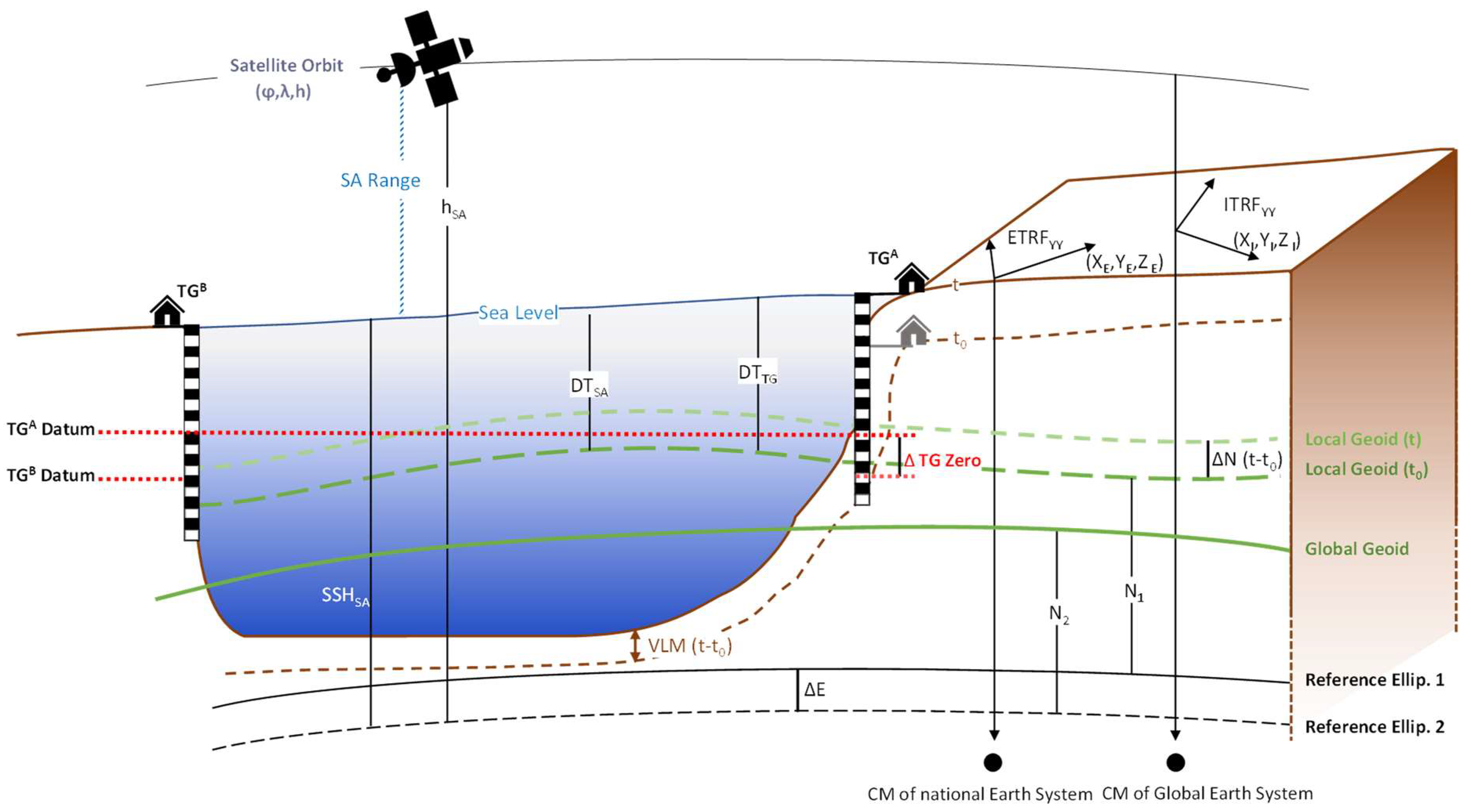
Conventions of the used DT data need to be considered in the development of the sea-level trend estimation methodology from the TG and SA observations. Modern TGs contain observation sensors, which automatically record the height of the coastal water level with high precision and temporal resolution (e.g., hourly). Contrastingly, the quality of historical TG records could be quite heterogeneous, due to the usage of mechanical mareographs or visual staff readings (e.g., twice a day). The TG zeros usually coincide with (or can be converted to) the zero of the vertical datum, which nowadays is often a geoid-based one [52]. Also, TG data could refer to different charts or national vertical data. Since the land-bound TG observations yield the RSL, which is the movement of the sea relative to land, to obtain ASL, the VLM effect needs to be removed from the TG observations (Figure 1). The SA-derived SSH is computed by subtracting the distance between the satellite altitude (determined in a global geocentric coordinate system) and the instantaneous sea surface. The SA data, therefore, are not VLM-affected, thus reflecting the true sea-level rise. Also, SA data are referenced to ITRF (e.g., realizations of 2008, 2014, etc.), while the regional/national geoid model could refer to another coordinate system, e.g., the ETRF (European Terrestrial Reference Frame). Hence, the aforementioned differences are necessary to be accounted for to achieve consistency in comparisons that contain SA and TG data.

To obtain the ASL-associated ${DT}_{TG}\left({\phi }_{TG},{\lambda }_{TG},t_i\right)$ at the location of the TG $({\phi }_{TG},{\lambda }_{TG})$, the TG observations $\left({DT}_{obs}\right)$ need to account for the VLM and geoid change (ΔN) corrections:

$${DT}_{TG}\left({\phi }_{TG},{\lambda }_{TG},t_i\right)={DT}_{obs}\left({\phi }_{TG},{\lambda }_{TG},t_i\right)+VLM\left({\phi }_{TG},{\lambda }_{TG}\right). (t_i-t_0)+\Delta N\left({\phi }_{TG},{\lambda }_{TG}\right). (t_i-t_0)$$

(1)

where the selected reference time epoch is denoted by $t_0$ and the TG observation time instant by $t_i$. The VLM value (denoted by $VLM\left({\phi }_{TG},{\lambda }_{TG}\right)$) and geoid changes (denoted by $\Delta N\left({\phi }_{TG},{\lambda }_{TG}\right)$) can be obtained from an appropriate VLM model. To obtain the TG-derived sea level, ${DT}_{TG@SA cycle}$, for the SA overfly instant, $t_{cycle}$, the ${DT}_{TG}$ data need to be selected within a predefined time window, w (before and after $t_{cycle}$). The matching TG data to the time instant, $t_{cycle}$, is estimated by the following linear (timewise) interpolation:

$${DT}_{TG@SA cycle}\left({\phi }_{TG},{\lambda }_{TG},t_{cycle}\right)=interp\left({DT}_{TG}\left({\phi }_{TG},{\lambda }_{TG},t_{cycle}\pm w\right)\right)$$

(2)

The instantaneous SA-derived along-track DT data point ${DT}_{SA}\left(\phi ,\lambda ,t_{cycle}\right)$ at an arbitrary location $\left(\phi ,\lambda \right),$ determine by subtracting the geoidal height ($N$) from the $SSH$ using the following expression:

$${DT}_{SA}\left(\phi ,\lambda ,t_{cycle}\right)=SSH\left(\phi ,\lambda ,t_{cycle}\right)-\Delta \mathrm{E}\left(\phi \right)-N\left(\phi ,\lambda \right)$$

(3)

where $SSH\left(\phi ,\lambda ,t_{cycle}\right)$ is the SA-derived instantaneous SSH data point by

$$SSH\left(\phi ,\lambda ,t_{cycle}\right)=h_{SA}-(R+\Delta R)$$

(4)

where $\Delta R$ are the necessary geophysical corrections that need to be applied to the SA range, $R$. Certainly, the outliers of the SA data must first be identified and removed from further computations using a certain method (e.g., see Section 4.1 for further details). Since initial datasets of different SA missions may refer to different reference ellipsoids, then ellipsoidal correction ($\Delta \mathrm{E}\left(\phi \right)$) for each SA data point is required. This ellipsoidal correction (associated with reference ellipsoid parameters) refers all participating SA measurements to the same reference ellipsoid [33].

For making the SA-derived DT comparable with ${DT}_{TG@SA cycle},$ a certain amount of the ${DT}_{SA}$ data points close the TG station for each SA mission and at each pass/cycle need to be spatially averaged to yield the following:

$${DT}_{SA@TG}\left({\phi }_{TG},{\lambda }_{TG},t_{cycle}\right)=\frac{1}{m}{\sum }_{j=1}^m{DT}_{SA}\left({\phi }_j,{\lambda }_j,t_{cycle}\right)$$

(5)

where $m$ is the number of j-th data points within the SA track segment up to a certain radius from each TG station. The resulting ${DT}_{TG}$, ${DT}_{TG@SA cycle},$ and ${DT}_{SA@TG}$ time series will be used for estimating the sea-level trends for each dataset. The most common method to estimate the sea-level trend is the ordinary least-squares (OLS) estimator [53,54,55,56]. The main advantages of using the OLS estimator for climate variables are that (i) it is consistent with previous estimators of sea-level trends and that (ii) the OLS estimate does not depend on the estimated variance–covariance matrix. This also means that the uncertainty estimates only depend on the variance–covariance matrix construction [13]. Hence, the linear regression model can be fitted to both SA and TG data to estimate the sea-level trend from each dataset. A linear model is defined as an equation that is linear in its coefficients:

$$Y\left(X\right)=\beta X+ϵ$$

(6)

where the model is denoted by Y(X), X is a suitable datum and $\beta$ is an unknown coefficient that can be estimated through OLS solution, and $ϵ$ is an unknown error (residual noise). The least-squares estimator of $\beta$ (denoted by $\widehat{\beta }$) can be derived as follows:

$$\widehat{\beta }~{\left(X^{t}X\right)}^{-1}{X}^{t}Y$$

(7)

In most cases, $\widehat{\beta }$ follows a normal distribution ($N\left(\mu ,{\sigma }^2\right)),$ where $\mu$ is the sample mean and ${\sigma }^2$ is the sample variance. The trend estimate uncertainty can be found by using the coefficient confidence. The coefficient confidence intervals (CIs) provide a measure of precision for regression coefficient estimates. A 100(1 − α)% CI gives the range that the corresponding regression coefficient will be within 100(1 − α)% confidence, meaning that 100(1 − α)% of the intervals resulting from repeated experimentation will contain the true value of the coefficient. The 100(1 − α)% CIs for regression coefficients are as follow [57]:

$$\widehat{\beta }\pm t_{\left(1-\alpha /2, n-p\right)}SE\left(\widehat{\beta }\right)$$

(8)

where $SE\left(\widehat{\beta }\right)$ is the standard error of the $\widehat{\beta }$ coefficient estimate (minimum error gives the best solution), $t_{\left(1-\alpha /2, n-p\right)}$ is the 100(1 − α/2) percentile of t-distribution with n–p degrees of freedom, n is the number of observations, and p is the number of regression coefficients (e.g., for 95% confidence, α = 0.05). In our case, a linear regression is fitted to the DT time series (for both SA- and TG-derived ones) to determine the sea-level trend estimates (the line slope $\beta$ shows the trend). The estimated $\beta$ now represents the sea-level trend (in mm/yr unit) (where $Y\left(X\right)=DT$ and $X=t$ in Equations (6) and (7)) and the corresponding uncertainties are obtainable using Equation (8).

Finally, the estimated (e.g., from SA data) and observed (e.g., from TG data) trends are statistically evaluated by using the root mean square error (RMSE):

$$RMSE=\sqrt{\frac{1}{n}{\sum }_{t=1}^n{({\beta }_t^o-{\beta }_t^e)}^2}$$

(9)

where $n$ is the total number of estimated trends during the study period; ${\beta }^e$ and ${\beta }^o$ are estimated (e.g., by SA) and observed (e.g., by TG) trend values at time $t$ (at different time windows), respectively.

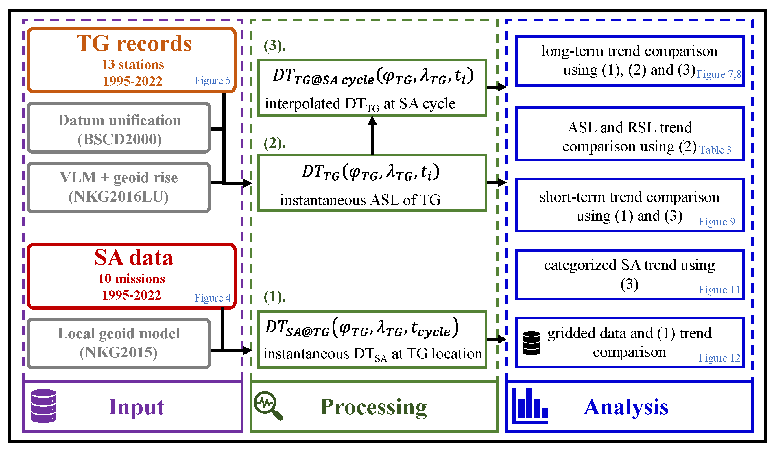
Note that the OLS-determined linear trend has its limitations, such as sensitivity to outliers, yielding extreme values and outliers which can skew the regression line and influence the estimated trend. Also, OLS assumes a linear relationship between the variables, which might not always represent the true nature of the sea level, especially over too-short periods. Hence, in this study, various non-linear methods, including the enveloping method [58] and sliding trend analysis [59,60] were additionally tested. These alternative approaches provided similar trend estimates to the OLS results. Therefore, for the sake of the conciseness of this paper, only the OLS-based linear trend estimation results will be explained and discussed. Figure 2 shows the flowchart of the applied methodology and data processing steps.

3. Study Area

The Baltic Sea is a semi-enclosed microtidal sea with geographical limits of 53°N–66°N and 10°E–30°E and roughly a 54 m mean depth, with a 393,000 km² total surface area. The sea is linked to the open ocean solely through narrow Danish Straits [61] (cf. Section 4.2). The sea-level dynamics of the Baltic Sea are affected by several meteorological and oceanographical components, including the variation in temperature, salinity, precipitation, and evaporation (in a decadal time frame), as well as extreme sea levels (in a short-time frame) as a result of storm surges due to the interaction of strong winds, waves, and pressure [62]. It features a dual stratification, marked by a seasonal thermocline in the summer and a persistent, robust halocline throughout the year. The halocline, at approximately 60–80 m, divides the brackish surface water with a salinity of about 7 psu from the deeper water, with 12 psu salinity. The surface salinities vary from 32 psu in the Kattegat to 1–2 psu in the northern parts [63]. Sequential (year to year) annual average sea-level variations in this region could exceed ±8 cm, whereas the maximum difference within the entire study period (1995–2022) could reach 25 cm, as presented in Figure A1. This large annual mean variation in sea level is challenging for short-term (decadal) sea-level trend estimations. The ASL of the Baltic Sea is also influenced by (i) expansion in the world ocean sea level (due to thermal seawater expansion and the melting of glaciers), which also propagates into the semi-enclosed Baltic Sea; (ii) low salinity, which causes an additional steric component, elevating the ASL specifically in the innermost parts of the sea, where the lowest densities occur; and (iii) local atmospheric forces, including wind and air pressure [33].

Over the past 50 years, previous studies have noted that the Baltic ASL increase is larger than the GMSL [63,64]. Also, the ongoing viscoelastic response of the Earth to the last deglaciation contributes to the sea-level variation in the Baltic Sea together with other effects such as North Atlantic and GMSL changes, wind, and waves affecting erosion and sediment transport [64]. Also, the spatial variations in the Baltic Sea level rates are mainly due to the (i) occasions of massive water entrance from the North Sea, (ii) intensified westerly winds, (iii) the poleward shift of low-pressure systems, and (iv) other minor contributions derived from local changes in baroclinicity, causing a basin-internal redistribution of water [64].

The changes in sea-level extremes depend on many variables, including storm surges [65], coastal upwellings [66], and wave-breaking processes [67], which can cause a devastating impact on small islands and their inhabitants. Hence, the cumulative effect of sea-level rises could lead to serious consequences over the Baltic Sea regions, where numerous archipelagos and small islands exist. Recent studies exploring future climate scenarios show an anticipated rise (around 6 mm/yr) in Baltic Sea levels (e.g., [29,30]). In contrast to the current study, many of these research works utilize gridded SA data or SLA for determining sea-level trends.

4. Datasets

This study determines RSL and ASL trends by using both TG (13 stations) and SA (10 missions) time series over the Baltic Sea for the period of 1995–2022. The beginning of the time series, 1995, considers the availability of reliable SA datasets.

4.1. Satellite Altimetry

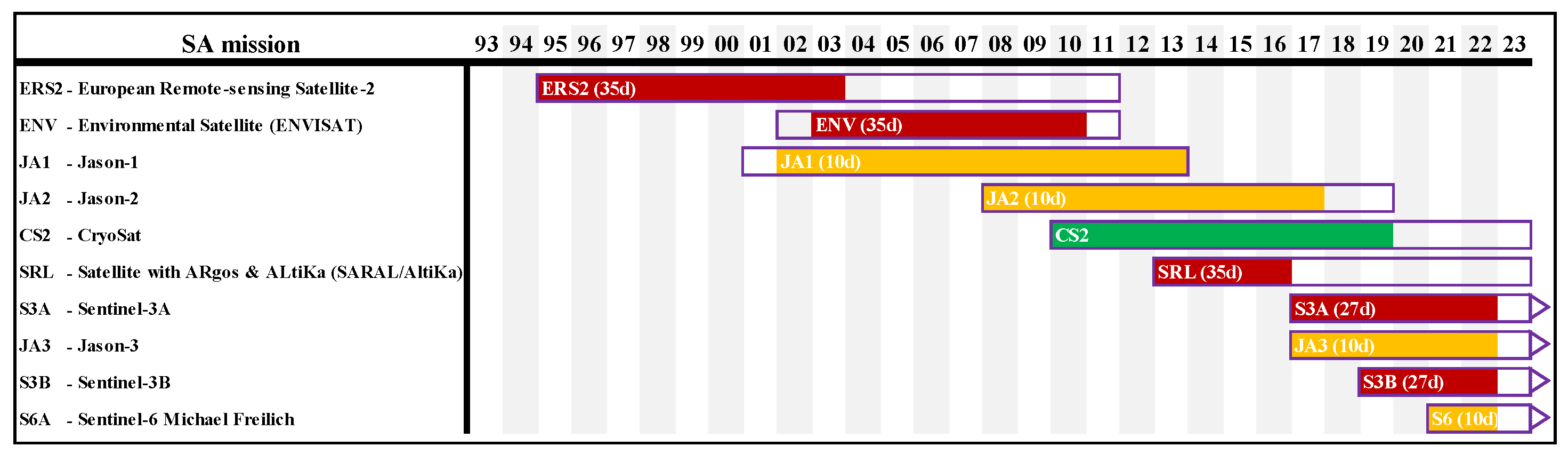
In this study, ten available SA missions’ data (Figure 3), including European Remote-Sensing Satellite-2 (ERS2), Envisat (ENV), Jason-1 (JA1), Jason-2 (JA2), Cryosat-2 (CS2), SARAL/AltiKa (SRL), Sentinel-3A (S3A), Jason-3 (JA3), Sentinel-3B (S3B), and Sentinel-6A Michael Freilich Jason-CS (S6A), are examined to determine the instantaneous ${DT}_{SA}$. These SA missions have different temporal coverage and resolution; see Figure 3 and

Table 1. Characteristics of the used SA missions (ordered by their launch dates) and related data spans.

ID	SA	Altitude [km]	Inclination [°]	Cycle [Days]	Data Frequency [Hz]	Data Period (Baltic + SEAL)		Data Period (Standard Data)
1	ERS2	785	98.5	35	20	16 May 1995	01 Jul 2003	-	-
2	ENV	800	98.5	35	18	18 Jun 2002	18 Oct 2010	-	-
3	JA1	1324	66	10	20	15 Jan 2002	20 Jun 2013	-	-
4	JA2	1324	66	10	20	12 Jul 2008	17 May 2017	-	-
5	CS2	717	92	w/o exact revisit cycle	20	19 Jul 2010	04 May 2019	-	-
6	SRL	800	98.5	35	40	14 Mar 2013	04 Jul 2016	-	-
7	S3A	814	98.6	27	20	04 Jan 2017	13 Jun 2019	13 Jun 2019	31 Dec 2022
8	JA3	1336	66	10	20	17 Feb 2016	31 May 2019	31 May 2019	31 Dec 2022
9	S3B	814	98.6	27	20	01 Nov 2018	19 May 2019	19 May 2019	31 Dec 2022
10	S6A	1336	66	10	20	-	-	1 Apr 2022	31 Dec 2022

. The highest-frequency SA data were used, i.e., distributed at a 20 Hz rate for most of the missions, except for 40 Hz for SARAL, and 18 Hz for Envisat.

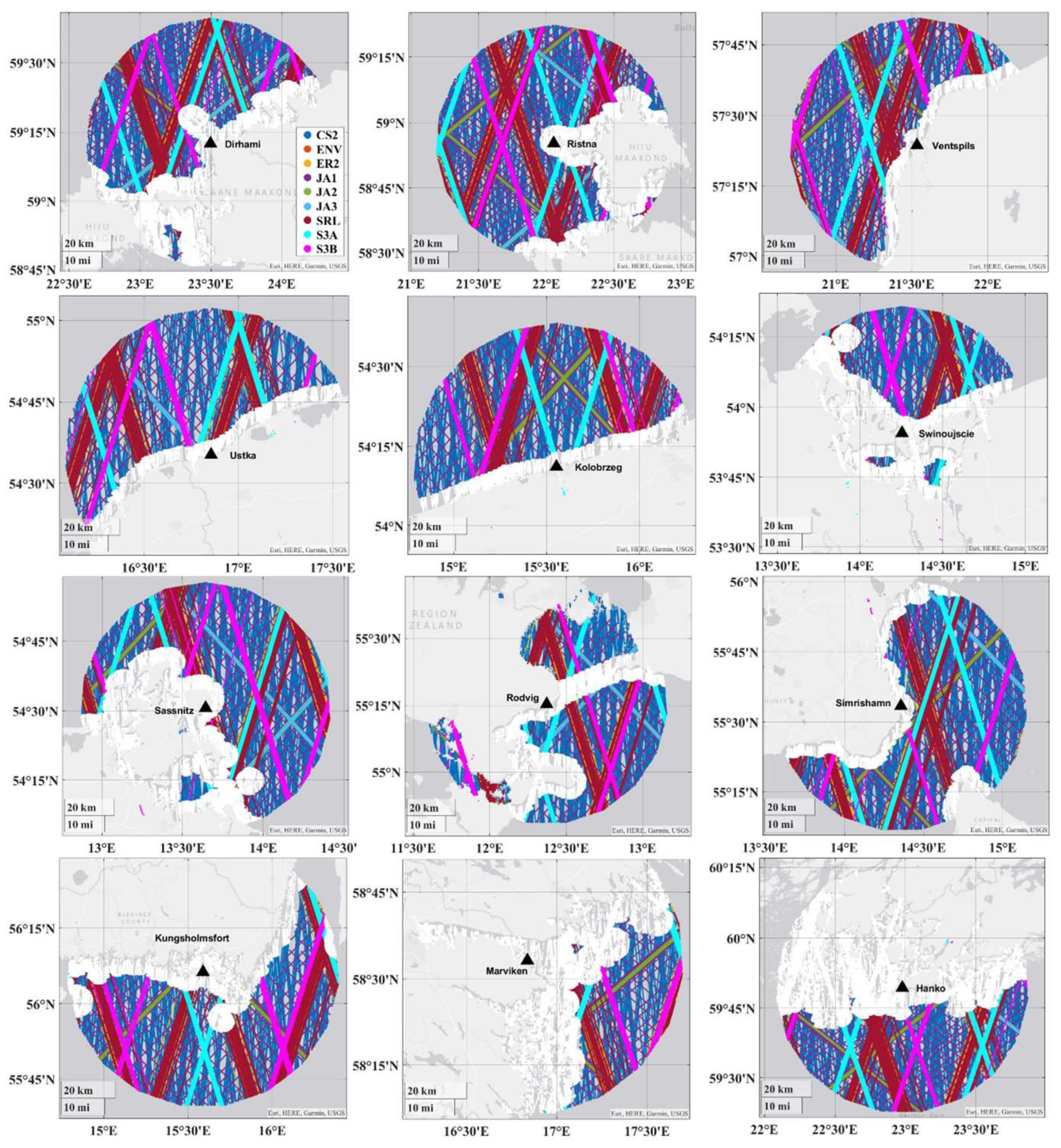
Compared to the open ocean, the SA data quality is degraded near the shoreline due to land contamination, seasonal sea ice conditions, and, possibly, erroneous corrections (e.g., wet tropospheric correction). Therefore, from the trend estimates of this study, the SA data points closer than 5 km to the shoreline were removed. Also, an iterative data screening approach [33] was applied to remove the outliers from the remaining SA data. Firstly, the gross errors ($\left|{DT}_{SA@TG}\right|>1.5 \mathrm{m}$) were removed from the SA datasets, followed by using median absolute deviation (MAD) for outlier detection. Figure 4 demonstrates the spatial distribution of the selected TG stations, which are mostly around the open parts of the sea (Baltic Proper) where more SA tracks can be acquired at these locations and has the smallest effect on ice coverage is apparent during the winter seasons (cf. [33]). High-quality SA along-track data were extracted up to 50 km from each TG station (see Figure 4). Equation (5) was then applied to obtain the averaged SA-derived DT estimates, whereas the number of SA data (m) varied from 1 to 326. In Figure 4, the selection of SA data at the location of the TG stations near the coast is illustrated, where the data points within 5–50 km from the shoreline of each SA mission are represented by different colours.

The European Space Agency’s Baltic + Sea Level (ESA Baltic + SEAL) Project dataset is an enhanced sea-level product that is specifically developed for the Baltic Sea [68]. However, this dataset contains the data only up to 2019; hence, in the present study, the “standard” EUMETSAT data were used to extend the trend estimation period from 2019 up to 31 December 2022. The Baltic + SEAL retracked data are available on request from http://balticseal.eu/outputs (accessed on 23 March 2021), whereas the standard data originated from the European Organization for the Exploitation of Meteorological Satellites (EUMETSAT), which can be downloaded from the EUMETSAT Earth Observation Portal at https://eoportal.eumetsat.int/ (accessed in 23 March 2023). The consistency of sea-level data from these two sources during the tandem phase of both datasets has been examined prior to our study. It should be noted that the former dataset includes a homogeneous estimate of multi-mission ASL, which has shown better results (as compared to the TG observations), rather than standard products [33]. Also, the necessary corrections (denoted by $\Delta R$) applied to all SA data consistently:

$$\Delta R=(\mathrm{w}\mathrm{e}\mathrm{t} \mathrm{t}\mathrm{r}\mathrm{o}\mathrm{p}\mathrm{o}\mathrm{s}\mathrm{p}\mathrm{h}\mathrm{e}\mathrm{r}\mathrm{i}\mathrm{c}+\mathrm{d}\mathrm{r}\mathrm{y} \mathrm{t}\mathrm{r}\mathrm{o}\mathrm{p}\mathrm{o}\mathrm{s}\mathrm{p}\mathrm{h}\mathrm{e}\mathrm{r}\mathrm{i}\mathrm{c}+\mathrm{i}\mathrm{o}\mathrm{n}\mathrm{o}\mathrm{s}\mathrm{p}\mathrm{h}\mathrm{e}\mathrm{r}\mathrm{i}\mathrm{c}+\mathrm{s}\mathrm{e}\mathrm{a} \mathrm{s}\mathrm{t}\mathrm{a}\mathrm{t}\mathrm{e} \mathrm{b}\mathrm{i}\mathrm{a}\mathrm{s}+\mathrm{s}\mathrm{o}\mathrm{l}\mathrm{i}\mathrm{d} \mathrm{E}\mathrm{a}\mathrm{r}\mathrm{t}\mathrm{h} \mathrm{t}\mathrm{i}\mathrm{d}\mathrm{e}+\mathrm{p}\mathrm{o}\mathrm{l}\mathrm{e} \mathrm{t}\mathrm{i}\mathrm{d}\mathrm{e}+\mathrm{r}\mathrm{a}\mathrm{d}\mathrm{i}\mathrm{a}\mathrm{l} \mathrm{o}\mathrm{r}\mathrm{b}\mathrm{i}\mathrm{t} \mathrm{e}\mathrm{r}\mathrm{r}\mathrm{o}\mathrm{r}+\mathrm{i}\mathrm{n}\mathrm{v}\mathrm{e}\mathrm{r}\mathrm{s}\mathrm{e} \mathrm{b}\mathrm{a}\mathrm{r}\mathrm{o}\mathrm{m}\mathrm{e}\mathrm{t}\mathrm{r}\mathrm{i}\mathrm{c} \mathrm{h}\mathrm{e}\mathrm{i}\mathrm{g}\mathrm{h}\mathrm{t}+\mathrm{D}\mathrm{A}\mathrm{C})-\mathrm{D}\mathrm{A}\mathrm{C}$$

(10)

Note that the dynamic atmospheric correction (DAC) on the right-hand side of Equation (10) denotes the removal of the DAC from the used SA datasets. Also, the ocean tide corrections are not included in the instantaneous SA data, considering that the TG data were extracted at the exact time instants of SA cycles. This makes the SA-derived DT compatible with TG records, which inherently contain the atmospheric pressure and the Baltic micro-tide contribution to the sea level. To achieve a consistent SA dataset, all the corrections were processed and applied uniformly, even though certain corrections may use different models (e.g., the wet tropospheric correction model varies depending on the Baltic + SEAL mission data). It was determined that the impact due to differences between these models is negligible for the SA-derived trend estimation.

The quality of SA data over the Baltic Sea is affected by two main features that limit the use of SA [33]: (i) the presence of sea ice and the proximity of the coast. For example, the northern part of the sea (62.1°N–65.8°N) is covered 110–190 days of the year by sea ice during the winter–spring seasons [69]. (ii) Also, the Baltic Sea contains the largest archipelagos in the world, with 30,500 islands and a 23 m average water depth only near Finnish coast [70]. Hence, this study focuses on the study area region (around the Baltic Proper), where these undesirable effects have the minimum impact on the SA sea-level trend estimates. The SA data need to account for other adjustments, including the permanent tide system [71] and the terrestrial reference frame unification. The ITRF transformation was carried out using the method explained by [72] in which the SA terrestrial reference frame is transferred from ITRF₂₀₀₈ or ITRF₂₀₁₄ to ETRF_YYYY, which is an ETRF realization of the year “YYYY” (e.g., 1995) related to the time epoch (YYYY) of the observations [33]. This includes marginal intra-plate velocity deformations and the transformation between ITRF and ETRF.

4.2. Tide Gauge Data

TG records provide an exclusive and comprehensive knowledge of sea-level changes and variations. However, they are land-bound, which means that the TG data reflect the RSL. Thus, to obtain the ASL, they need to correct for the VLM effect. In this study, the TG-derived ASL is compared with the SA-derived ASL trend estimates. The Baltic Sea has one of the world’s densest observational tide gauge networks with remarkably long-term and high-quality local sea-level records [73]. Within the study area, 13 TG stations were selected that match the time span (1995–2022) of available SA data. Most TG stations provide hourly data for the entire study period, whereas a couple of used stations had only a few daily readings within the first decade of the study period. Some of the TG stations have longer data gaps due to the malfunctioning or change of the sensors; for more details, see

Table 2. Overview of the used TG data for the study period from 1 January 1995 to 31 December 2022. Significant (>18%) data gaps are highlighted in bold font.

ID	Station	Latitude [°]	Longitude [°]	Country	VLM [mm/yr]	$\mathbf{\Delta }\mathit{N}$ [mm/yr]	No. Hourly Data (i)	Missing Hourly Data [%]
1	Dirhami	59.21	23.50	Estonia	3.09	0.4	117,833	51.99 1
2	Ristna	58.92	22.06	Estonia	3.46	0.4	244,427	0.42
3	Ventspils	57.40	21.53	Latvia	1.56	0.3	200,199	18.41
4	Ustka	54.59	16.85	Poland	0.13	0.1	175,622	28.45
5	Kolobrzeg	54.19	15.55	Poland	−0.06	0.1	170,399	30.58
6	Swinoujscie	53.91	14.25	Poland	−0.18	0.1	175,157	28.64
7	Sassnitz	54.51	13.64	Germany	0.09	0.1	237,694	2.58
8	Rodvig	55.25	12.37	Denmark	0.62	0.2	226,479	7.73
9	Simrishamn	55.56	14.36	Sweden	0.89	0.2	234,745	0.00
10	Kungsholmsfort	56.11	15.59	Sweden	1.36	0.2	245,439	0.00
11	Marviken/Arkö 2	58.55	16.84	Sweden 3	4.46	0.4	245,448	0.00
12	Hanko	59.82	22.98	Finland	4.16	0.4	245,448	0.00
13	Pori	61.59	21.46	Finland	7.44	0.7	244,728	0.29

¹ Dirhami TG station includes visually recorded historical data twice a day up to 2010; consequently, the overall number of missing hourly data is the highest for this TG station. Hence, up to 2010, the maximum time span between the TG reading and the SA flyover instant could reach up to 6 h. From 2011 onward, the hourly observations from a pressure sensor are available. ² The tide gauge Marviken was operational up to 10 January 2019; hence, another station close (~10 km) to this TG is used for the remaining time period: Arkö station, with a latitude of 58.4843° and a longitude of 16.9607°. ³ All Swedish stations have manual data recording up to 2004, cf. Table A1.

and

Table A1. History of measurement devices for each TG station.

ID	Station	Measurement Device History	Data Provider
1	Dirhami	01.01.1995–30.04.2009: manual observations, twice a day at 06 and 18 UTC. 21.09.2010–present: high-precision-level sensor PAA-36XW/H from Keller AG.	www.keskkonnaagentuur.ee
2	Ristna	01.01.1995–24.09.2010: mareograph. 22.09.2010–present: high-precision-level sensor PAA-36XW/H from Keller AG.
3	Ventspils	23.02.1996–25.08.2004: HMS—1820 sensor from MARIMATECH 26.08.2004–13.09.2011: OTT ODS sensor from OTT HydroMet. 14.09.2011–present: OTT PLS sensor from OTT HydroMet
4	Ustka	1995–2015.12.1: Limnigraph LPU-10 from Zootechnics 2005.09.01–2023.07.05: Float Telemetry from Sutron 2023.07.06–present: Pressure sensor DST 22 from Seba	www.imgw.pl
5	Kolobrzeg	1995–2009.06.01: Limnigraph LPU 10 Zootechnics 2009.01.07–2012.04.30: Limnimeter ORPHEUS from OTT 2004.05.19–2023.08.23: Float Telemetry Xlite 9210 from Sutron 2023.08.24–present: HD-01 from Envag
6	Swinoujscie	1995–2015.12.2: Limnigraph LPU-10 from Zootechnics 2006.02.08–2019.06.26: Float Telemetry from Sutron 2019.06.27–2023.09.24: OTT PLS device (subpress) from OTT 2023.05.09–present: Pressure sensor DST 22 from Seba
7	Sassnitz	1970–1996: STEREMAT-Recording Stage indicator (Model 195109) 01.06.1996–2013: angle encoder from Rittmeyer and beginning of water level remote transmission. 20.10.2013–present: Ott-Hydromet pressure sensor (Model 194772) as redundant system.	www.bsh.de
8	Rodvig	1995–February 2015: Data collected by Farvandsvæsenet institute and not enough details of the instruments are available. February 2015–October 2021: CBS–Compact Bubbler Sensor by OTT October 2021–present: Radar measurement Time-of-Flight Micropilot FMR52 from Endress	www.dmi.dk
9	Simrishamn	1995–07.08.2004: Float measurement collection, data manual dialling of the station (telepegel). 07.08.2004–15.05.2018: Shaft encoder AD150A 2018.05.15–Present: Radar Vega puls61	www.videscentrs.lvgmc.lv
10	Kungsholmsfort	1995–08.07.2004: Float measurement collection, data manual dialling of the station (telepegel). 28.11.2002–12.11.2018: Shaft encoder AD150A. 12.11.2018–Present: Radar Vega puls61.
11	Marviken/Arkö	1995–07.08.2004: Float measurement collection, data manual dialling of the station (telepegel). 03.05.2004–01.10.2019: Shaft encoder AD150A (station closed). 29.08.2017–Present: Radar Vega Puls 61 (from 01.10.2019, Arkö data are used).

and Figure 5b.

The selected TG stations are operated by the national tide gauge authorities. The TG readings refer to the corresponding national realization of the EVRS2000 (European Vertical Reference System 2000) vertical datum (e.g., [74]), the zero level of which is the Normaal Amsterdams Peil (NAP). In addition, the TG zero level was transformed into the mean permanent tide system. The locations of TG stations are shown in Figure 5, where the VLM effect is illustrated in the background and the geoid rise ($\Delta N$) is also shown with red isolines; for more details, see Section 4.4.

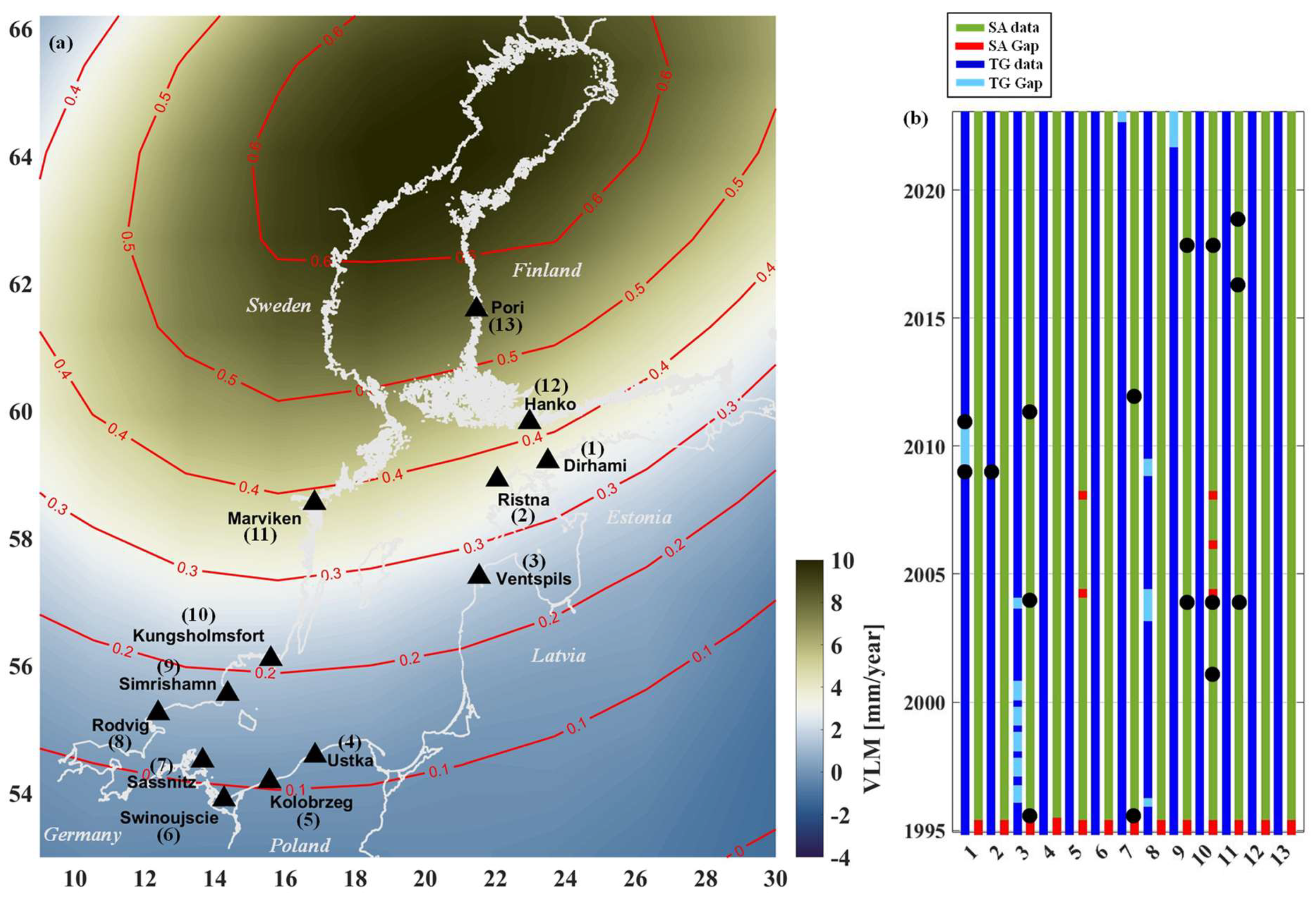
Figure 5. TG stations used in this study: (a) VLM rate [mm/year] over the Baltic Sea region according to the NKG2016LU model [75]. The geoid changes (rise over the Baltic Sea) [mm/yr] are also shown with red isolines. The numbered triangles denote the location of TG stations used in this study. (b) TG (blue) and SA (green) monthly data availability during the study period at each TG station (TG monthly averaged data are used for illustration). Gaps of data are illustrated in different colours (TG data gaps in light blue and SA data gaps in red). The black dots represent the TG sensor installation events (full details in Table A1).

Figure 5. TG stations used in this study: (a) VLM rate [mm/year] over the Baltic Sea region according to the NKG2016LU model [75]. The geoid changes (rise over the Baltic Sea) [mm/yr] are also shown with red isolines. The numbered triangles denote the location of TG stations used in this study. (b) TG (blue) and SA (green) monthly data availability during the study period at each TG station (TG monthly averaged data are used for illustration). Gaps of data are illustrated in different colours (TG data gaps in light blue and SA data gaps in red). The black dots represent the TG sensor installation events (full details in Table A1).

All the available TG hourly data were used for the ASL and RSL trend estimates as the ground truth. Note that the SA-derived ${DT}_{SA@TG}\left({\phi }_{TG},{\lambda }_{TG},t_{cycle}\right)$ is also compared with ${DT}_{TG@SA cycle}$ in order to examine whether the SA data random and diverse temporal sampling is sufficient for deriving the SA-based ASL trend estimates. Therefore, to obtain ${DT}_{TG@SA cycle}$ using Equation (2), the ${DT}_{TG}$ readings only within 2 h before and after the $t_{cycle}$ time window (resulting in a total duration of 5 h for w) are included in the temporal interpolation (TG records beyond this specified time window are excluded). Consequently, if there is a gap in the TG record within the time window, w, the resulting ${DT}_{TG@SA cycle}$ remain as a NaN value. In other words, in ${DT}_{TG@SA cycle}$- and ${DT}_{SA@TG}$-based sea-level trend estimates, different DT values may participate; such discrepancies are addressed later, in Section 5.3.2. It is important to note that there might be a gap in the TG precisely at $t_{cycle}$. However, employing ${DT}_{TG@SA cycle}$ allows us to effectively represent the DT derived from TG, considering the relatively low fluctuations in DT within the w time frame.

Note that, during the study period, four TG stations had significant data gaps (cf. Table 2) which may negatively affect the TG-derived sea-level trend estimates. For instance, for the Dirhami (#1) station, sea-level data were visually captured twice a day up to end of 2009; for the entire year 2010, there were no data record at all, whereas the hourly TG data records started from 2011. The monthly averaged TG data enable the detection of longer data gaps in the TG and SA time series; see Figure 5b, which may be different from the instantaneous data gap (mentioned in Table 1). In this study, the longest data gap (Dirhami) reaches up to one year.

4.3. Geoid Model

The regional NKG2015 quasi-geoid model [76] was used to retrieve ${DT}_{SA}$ from SA-derived SSH data, as explained in Section 2. It is referred to as the Geodetic Reference System 1980 (GRS80) ellipsoid and covers the area from 53° to 73°N and from 0° to 34°E, with a grid spacing of 0.01° × 0.02°. NKG2015 has a good agreement with GNSS/levelling control points, with a standard deviation (STD) of 3.0 cm [76]. Various studies have estimated the NKG2015 geoid error that could reach up to 15 cm over certain marine areas. Such deficient geoid modelling areas were associated with the poor coverage of marine gravity data. Contrastingly, the global geoid models that are customarily used by the satellite altimetry community are less accurate and with a poorer spatial resolution (typically 0.1° × 0.1°, e.g., EGM2008). It should be noted that the geoid model deficiencies do not affect the trend estimation studies; however, a precise geoid is needed for the examination of oceanographic processes (e.g., [50,51]). Although, the geoid model may also be constrained by some problematic areas, which were investigated by [33,51]. These areas are avoided in this study.

4.4. Vertical Land Motion and Geoid Rise Models

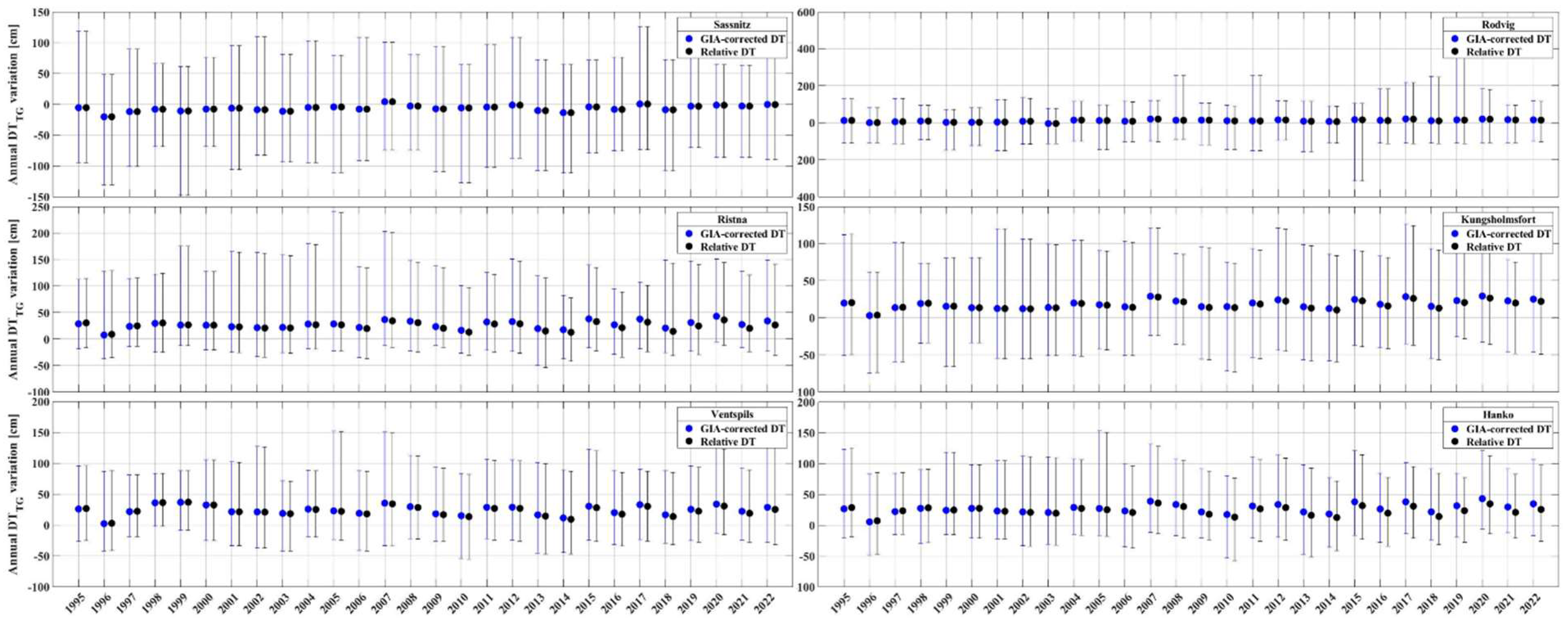
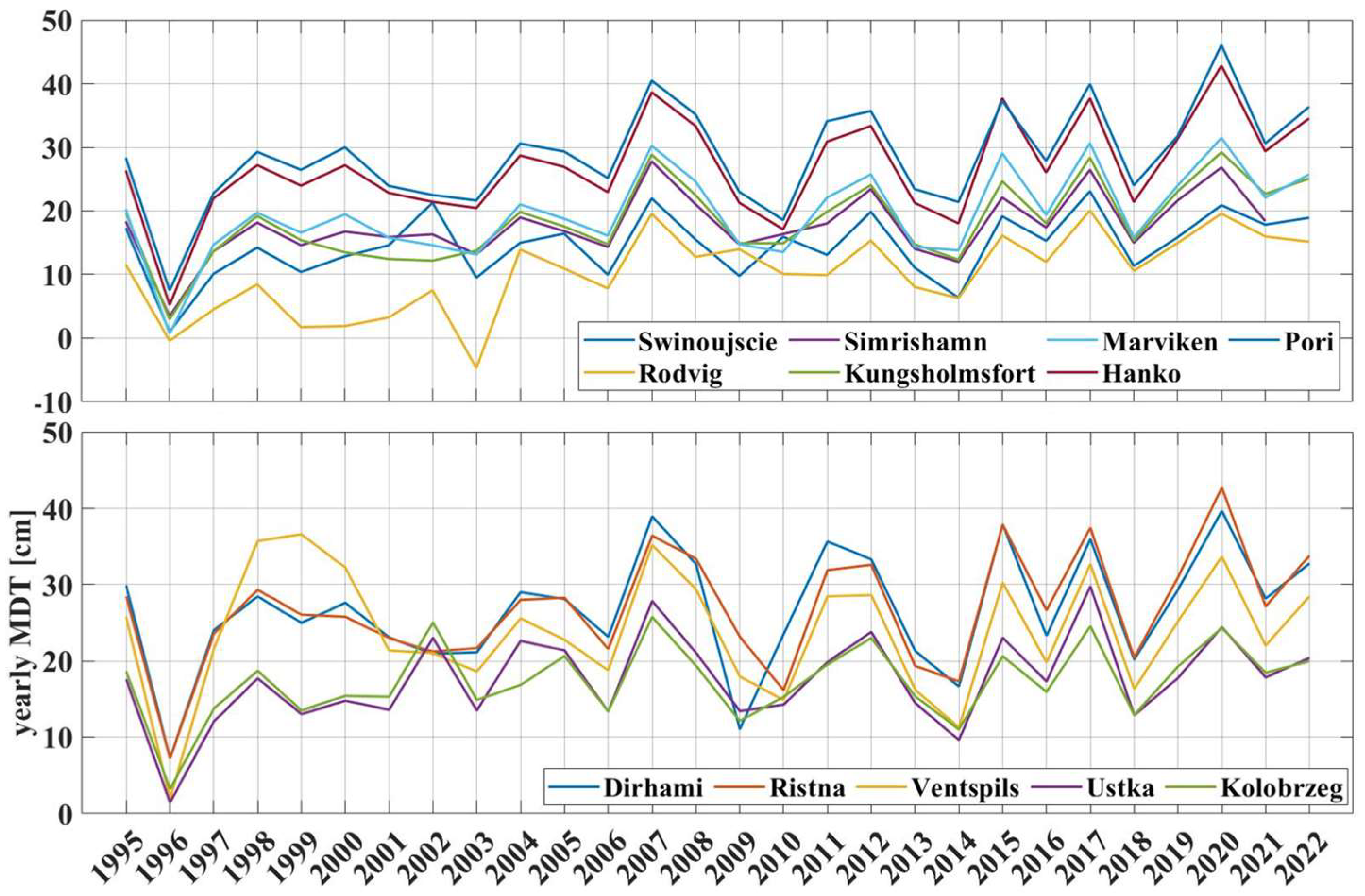
In order to obtain the ASL trend values from the TG-derived RSL, the VLM needs to be considered. VLM may occur due to glacial isostatic adjustment (GIA), tectonic motion, and anthropogenic effects. Over the Baltic Sea region, VLM is dominated by GIA, caused by ice shield melting after the last deglaciation over the Fennoscandia. Slow crustal recovery from the pressure of the ice sheet that covered the area during the last glacial period causes post-glacial land uplift up to around 10 mm/yr in the north part of the sea (centre of the former ice sheet) and decreases to nearly zero at the edges of the former ice sheet (south). The southern part of the Baltic Sea therefore experiences a land subsidence as a compensating effect. This causes the RSL to increase in the north and decrease in the south part of the Baltic Sea, as can be seen from TG records (cf. Figure 5 and Figure 6). In recent decades, an acceleration has been seen in the long-term sea-level trends since the 1960s [77], consistent with the global signal [2]. On the other hand, SA and GPS (Global Positioning System) provide independent measurements of sea-level change and VLM, with respect to a global geocentric coordinate system. To assess the separate effects of sea-level change and land uplift, accurate information on land uplift is essential in the Baltic Sea region, as the VLM value varies throughout the region. In this study, the land uplift effect is removed from TG observations using the NKG2016LU model to convert the TG readings (${DT}_{obs}$) to the actual DT (${DT}_{TG}$), i.e., relative to the Earth’s centre of mass. This model includes the latest GIA land uplift model for the Baltic Sea region, developed by the Nordic Commission of Geodesy (NKG, www.nordicgeodeticcommission.com (accessed on 26 August 2021), and it covers an area from 49° to 75°N and 0° to 50°E [75]. The VLM correction reference time epoch (i.e., $t_0=2000.0$) is applied to the TG observation time record (i.e., $t_i$) by adding it to the TG readings using Equation (1). Also, the geoid change ($\Delta N$) is primarily due to GIA, which causes a rise in the geoid in the Baltic Sea (cf. Figure 4). The $\Delta N$ rate is approximately 10–15% of the VLM rate in the Baltic Sea [34]. Figure 6 shows annual DT variations of TG observations (hourly data) before (black) and after (blue) VLM correction for six selected TG stations.

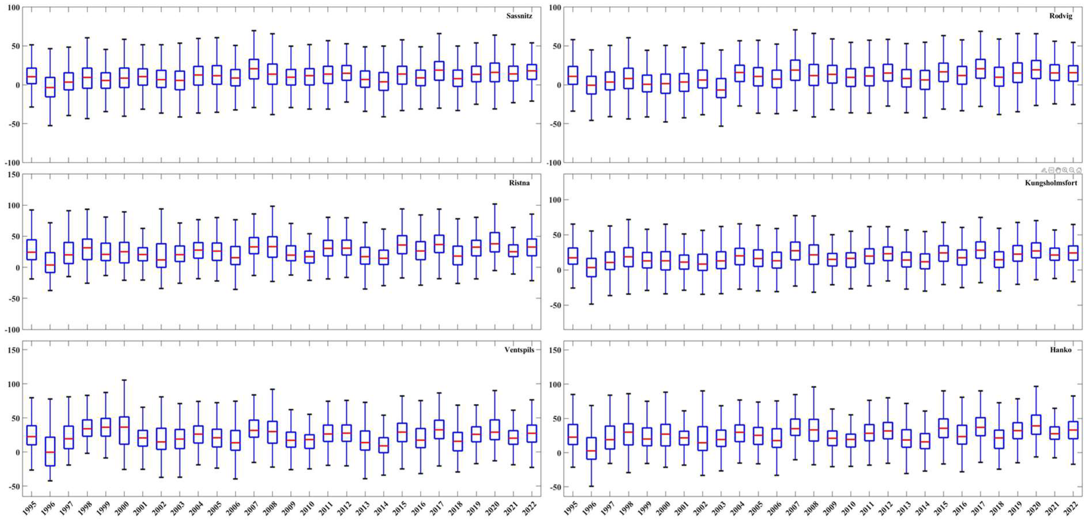
In this study, both RSL and ASL are considered for trend estimation, as illustrated in Figure 6 (RSL in black and ASL in blue dots) to illustrate the VLM effect. This figure shows the annual DT variation of six selected TGs (one for each country), for example, before (black) and after GIA correction (blue). Accordingly, a significant deviation of ASL and RSL can be observed over intense land uplift areas (e.g., the Pori and Hanko stations), as was expected. The dots show the average DT of each year, and the bars represent the maximum and minimum DTs, whereas the STD of the annual MDT value varies within 5 to 8 cm. Additionally, the annual fluctuation in MDT, calculated as the difference between the maximum and minimum MDT values for each year, ranges from 20 to 30 cm during the period from 1995 to 2022 across all stations. These significant fluctuations in annual MDT could result in a notably high degree of variability in estimated sea-level trends, particularly when using short-term time-series data. Also, Figure A2 represents the median values and the 25th and 75th percentiles of the annual DT variations for six stations (the same as in Figure 6).

4.5. Model Data

To validate our ASL trend estimation method, we conduct an additional examination using standard products that have been used in earlier studies. Hence, in addition to instantaneous along-track SA and TG data, three monthly gridded model data were employed to estimate the trends which are discussed in Section 5.4.3. These datasets are as follows:

• Global SA gridded SLA (https://doi.org/10.48670/moi-00148 (accessed on 9 October 2023)) computed with respect to a twenty-year 1993–2012 mean from the Copernicus Marine Data Store (www.data.marine.copernicus.eu (accessed on 9 October 2023)): This SLA (denoted as global gridded SLA in Section 5.4.3) is estimated by Optimal Interpolation, merging the Level-3 along-track measurement from the different available SA data. This product is processed by the DUACS (Data Unification and Altimeter Combination System) multi-mission altimeter data processing system.
• The Baltic Sea Physical Reanalysis product (https://doi.org/10.48670/moi-00013 (accessed on 15 May 2023), which provides a reanalysis of the physical conditions of the whole Baltic Sea area: The product (denoted by Baltic Sea Nemo, gridded in Section 5.4.3) is produced by using the ice–ocean model system Nemo. The data are available at the native model resolution (1-nautical-mile horizontal resolution, 56 vertical layers).
• Baltic + SEAL gridded SA data over the Baltic Sea region: This product provides SSH after the multi-mission cross-calibration and outlier detection [29]. In this product, the SA observations are interpolated on an unstructured triangular grid (i.e., geodesic polyhedron) with a spatial resolution of 6–7 km.

It is important to consider that these models may have challenges related to vertical data incoherency (e.g., [33,50,51]). However, it needs to be emphasized that despite potential discrepancies in the vertical data, these issues are not anticipated to significantly impact the outcomes of sea-level trend estimations.

5. Results

This section presents the estimated sea-level trends for locations within the Baltic Sea region. Given the variations in data sources and time spans considered, four main aspects are examined: (i) long-term (1995–2022) relative sea level (RSL) and absolute sea level (ASL) trends are calculated using only hourly TG data at each station (Section 5.1), (ii) a comparison of long-term ASL estimates by both TG and along-track SA (Section 5.2), (iii) a comparison of decadal ASL trend estimates by TG and SA (Section 5.3), (iv) and inter-comparisons of the estimated SA-based trend (Section 5.4), which includes an examination of ASL sea-level trend calculations using different distances from the coast (Section 5.4.1), an examination of ASL calculated using different SA missions (Section 5.4.2), and a comparison of ASL trend estimates using other available sea-level datasets (Section 5.4.3).

5.1. ASL and RSL Trends by Hourly TG Observations

The long-term (1995–2022, 28 years) RSL and ASL trends were calculated using hourly data of ${DT}_{obs}$ and ${DT}_{TG}$ (VLM-corrected) based on Equation (6) (Section 2). The achieved RSL and ASL rates and their uncertainty from TG observations for the period 1995 to 2022 are listed in

Table 3. TG hourly data based on RSL and ASL estimates, their formal OLS-based uncertainties, and mean dynamic topography (MDT) of hourly TG observation [cm] for each station (during 1995–2022).

ID	Station	MDT [cm]	ASL Trend [mm/yr]	RSL Trend 1 [mm/yr]	ASL–RSL Difference [mm/yr]
1	Dirhami	29.03	3.58 ± 0.024	0.49	3.09
2	Ristna	26.87	4.56 ± 0.012	1.11	3.45
3	Ventspils	23.73	2.12 ± 0.014	0.56	1.56
4	Ustka	18.46	2.36± 0.014	2.22	0.14
5	Kolobrzeg	18.10	2.06 ± 0.014	2.12	−0.06
6	Swinoujscie	15.29	2.66 ± 0.014	2.84	−0.18
7	Sassnitz	10.66	3.22 ± 0.010	3.13	0.09
8	Rodvig	10.55	5.13 ± 0.011	4.51	0.62
9	Simrishamn	17.60	3.55 ± 0.010	2.66	0.89
10	Kungsholmsfort	18.34	4.81 ± 0.009	3.45	1.36
11	Marviken	19.57	4.90 ± 0.009	0.44	4.46
12	Hanko	26.79	5.37 ± 0.011	1.21	4.16
13	Pori	28.67	5.41 ± 0.011	−2.02	7.43

¹ Note that the RSL trend uncertainties are the same as for the corresponding ASL.

and Figure A3.

In general, the RSL varies within the magnitude of −2 to 4.5 mm/yr, while the ASL rate spans from 2 to 5.4 mm/yr. Another notable characteristic is the spatial variance among the stations, mainly due to the VLM effect (cf. Figure A3 and Table 2). It is evident that the largest differences between RSL and ASL are observed at the northern stations, which tend to experience large VLM effects, for example, at stations Dirhami (0.49 vs. 3.58 mm/yr), Ristna (1.11 vs. 4.56 mm/yr), Marviken (0.44 vs. 4.9 mm/yr), Hanko (1.21 vs. 5.37 mm/yr), and Pori (−2.02 vs. 5.41 mm/yr). Note the opposite trend sign for the (northernmost) Pori TG station, where the land uplift exceeds the sea-level rise. Note that the differences between the ASL and RSL rates (cf. Table 3, last column) are almost equal to the VLM at these locations (cf. Table 2, sixth column). This validates the reliability of our trend estimation methodology.

Previous studies have also observed a decreasing RSL trend toward the north, whereas the ASL trend increased toward the south [29,45,46,78]. Note that, in various studies, the trend estimates may differ due to the adoption of the time period examined, the source of measurement, the method of computation, and the exact locations of measurement. For instance, within the same region, [78] estimated an RSL within the approximate range of −8 to 1 mm/yr. In the study by [45], a similar range of RSL trends was calculated using a TG and hydrodynamic model (HDM) for the period 1915 to 2014. The ASL trends varied from 1 to 6 mm/yr, a range similar to what was observed by [29] using gridded monthly SA and TG data. These results indicate that, despite the differences in time frames and the sources of sea-level data (such as TG, HDM, SA), the long-term sea-level trends calculated across these studies generally align. These studies also verify the importance of accounting for the VLM in sea-level trend studies. This prompts the question as to whether any major difference truly occurs between utilizing TG and SA data sources for sea-level trend estimations, and whether computing sea-level trends over shorter periods, like decades, yields comparable values. These questions are examined in the following sections.

5.2. Long-Term ASL Trend

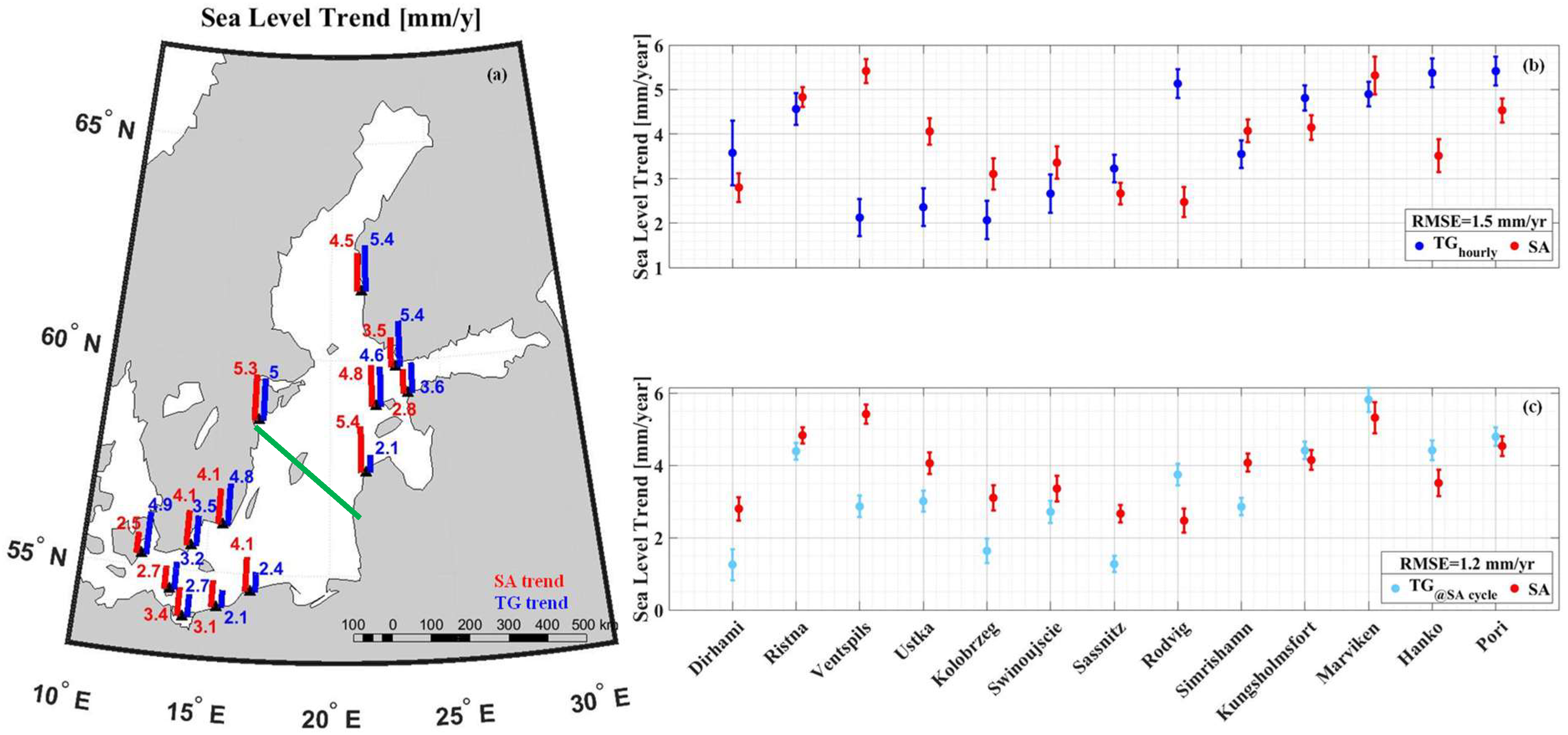
The long-term (1995 to 2022) ASL trend results using both SA and TG are illustrated in Figure 7. The ASL trends are calculated using (i) hourly TG observations (dark blue); (ii) TG-derived ${DT}_{TG@SA cycle}$ (light blue); and (iii) SA instantaneous data (red). The RMSE of the paired estimates for all stations are computed by Equation (10), where ${\beta }^o$ is either ${trend(DT}_{TG})$ (Figure 7b) or ${trend(DT}_{TG@SA cycle})$ (Figure 7c), whereas ${\beta }^e={trend(DT}_{SA})$.

The comparison of the TG and SA sea-level trends also reveals a spatial variability among the stations (Figure 7 and Figure 8). In the north-eastern study area, certain stations (such as Pori, Hanko, Ristna, and Marviken) exhibit higher sea-level trend values (observed in both SA and TG) ranging around 4 to 5 mm/yr. Previous studies have also noted larger ASL trends in the north-eastern Baltic Sea region (e.g., [29,45,46,63]). This was suggested to be attributed to fluctuations in air pressure [79,80] and intensified westerly winds that push the water masses toward the north-east [29,63]. Additionally, a poleward shift in low-air-pressure systems was observed, contributing to local sea-level increases via the inverted barometer effect. Moreover, an increased influx of freshwater from the northern Baltic Sea has been suggested as a factor leading to the rise in the mean sea level over the northern and western Baltic Sea sections [63]. However, within the south-western section, the trend values mostly varied between 2 and 4 mm/yr. Notably, stations Rodvig (#8) and Kungsholmsfort (#10) revealed large TG-derived trend values of nearly 5 mm/yr (Figure 7).

At most stations, the sea-level trends of ${DT}_{SA@TG}$ and ${DT}_{TG}$ data (Figure 7b) vary from 2.1 to 5.4 mm/yr. A closer examination of individual stations in Figure 7b reveals that 9 stations (out of 13) agreed within ±1 mm/yr. The most notable differences appear to occur at stations Ventspils (#3, with a difference of 3.3 mm/yr), Ustka (#4, difference of 1.7 mm/yr), Rodvig (#8, with a difference of 2.6 mm/yr), and Hanko (#12, with a difference of 1.9 mm/yr) (cf. Figure 7b). Similarly, the ${DT}_{SA@TG}$ and ${DT}_{TG@SA cycle}$ trends (Figure 7c) vary overall from 1.3 to 5.8 mm/yr. The differences in the ${DT}_{SA@TG}$ and ${DT}_{TG@SA cycle}$ trends in Figure 7c indicate that out of the 13 stations assessed, only the trends of six stations remain within a ±1 mm/yr tolerance. Broadening the allowable differences to ±1.5 mm/yr, however, revealed that 11 out of 13 stations are in agreement. The largest differences were determined at the TG stations Rodvig (#8) and Kolobrzeg (#5), with 2.5 mm/yr and 1.5 mm/yr, respectively.

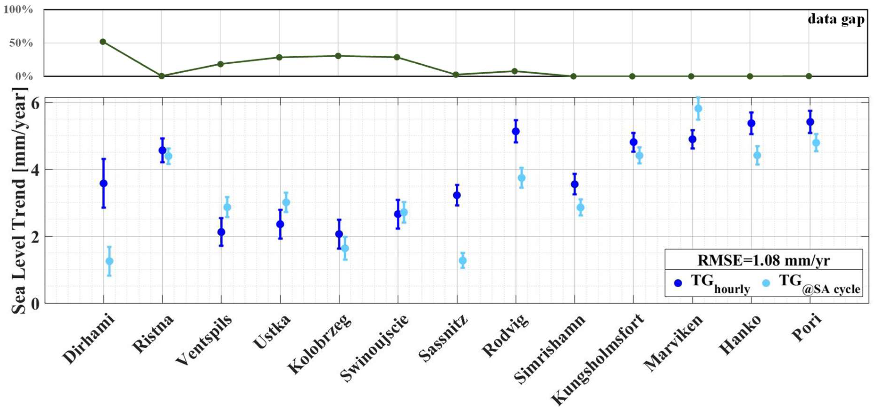
Further examination suggests that large differences within the range of 1–1.5 mm/yr may indicate issues with the SA or TG data for these specific stations. For instance, trend estimates are potentially affected by extensive data gaps (cf. Table 2, Figure 8) in stations such as Dirhami (#1), Ventspils (#3), Ustka (#4), Kolobrzeg (#5), and Swinoujscie (#6). Moreover, upon examining individual stations, it became evident that the ${DT}_{SA@TG}$ and ${DT}_{TG}$ pairs tended to yield more reliable results, showing agreement within a difference of ±1 mm/yr. Figure 7a,b show that the ${DT}_{SA@TG}$ and ${DT}_{TG@SA cycle}$ pairs display slightly improved agreement, with an RMSE of 1.2 mm/yr, compared to that of the ${DT}_{TG}$ and ${DT}_{SA@TG}$ pairs, which yield an RMSE of 1.5 mm/yr. Also, the overall average ASL trend of the 13 stations is 3.9 mm/yr using favourably hourly TG data, whereas utilizing instantaneous (but time-wise irregular) SA data yields a trend estimate of 4.8 mm/y in the Baltic Sea. This experiment demonstrates that the temporal frequency of the instantaneous SA data could be sufficient for sea-level trend estimates, yielding an agreement of ±1 mm/yr with the hourly TG data series (cf. Figure 8).

Figure 7b,c suggest that SA data stand out as a dependable method to accurately determine ASL trends in proximity to the coast, with an accuracy of 1 to 1.5 mm/yr. This is of particular significance given the challenges associated with obtaining precise sea-level estimates in these coastal areas, especially within the unique characteristics of the Baltic Sea [33]. Moreover, it highlights the constraints of TG data for estimating RSL trends, especially for stations with missing data. While, historically, TG data records have been extensively utilized for sea-level trend determinations, the presence of data gaps and outliers can lead to distorted trend estimates, particularly on a regional scale. Therefore, SA data emerge as a reliable resource for determining sea-level trends on a regional scale, particularly over such areas where the quality or presence of TG stations may be insufficient.

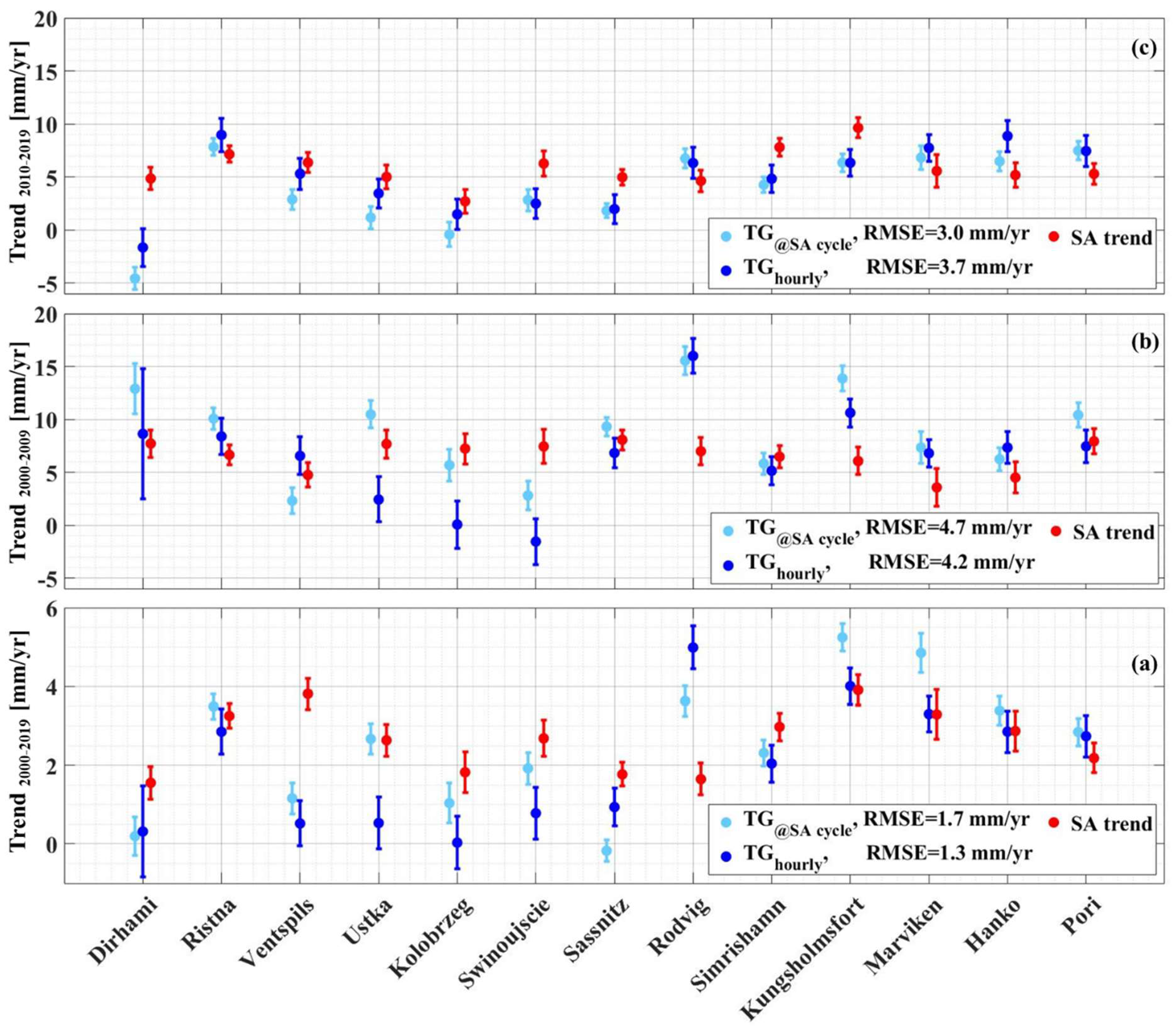
5.3. Decadal Regional ASL Trend

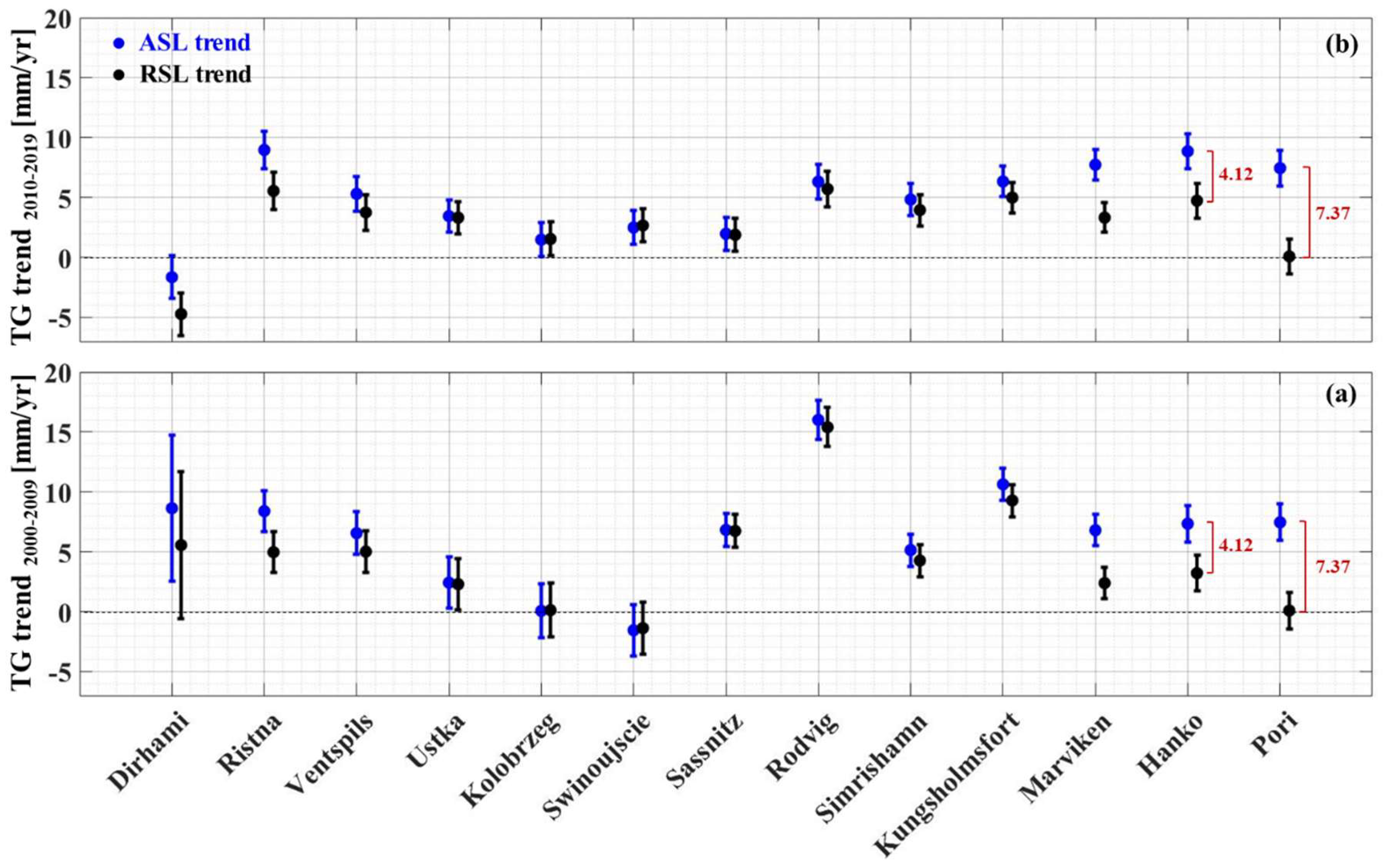
The decadal SA-derived ASL trend was examined and compared with TG for two distinct periods—1 January 2000 to 31 December 2009 and 1 January 2010 to 31 December 2019—using the OLS-estimated linear trend (Equations (6) and (7)). The outcomes are presented in Figure 9, employing various DT calculations such as instantaneous SA data (${DT}_{SA@TG}$), hourly TG data (${DT}_{TG}$), and TG data at the time of the SA cycle (${DT}_{TG@SA cycle}$). While all three methods yielded slightly different results (as detailed in Section 5.3.2), several main characteristics remained consistent across all approaches. These are described below in terms of (i) a comparison with the long-term trends (1995–2022) and (ii) a comparison between the different decades.

5.3.1. Comparison between Long-Term and Decadal Trends

By comparing the decadal (2000–2009 and 2010–2019) trends with the long-term trend, two major observations emerged: Firstly, both decades revealed a spatial variation in sea-level trend among the stations. The northern stations (stations #1, #2, #3, #11, and #13) exhibited higher rates compared to the southern (#4, #5, #6, and #7) and western stations (#8, #9, and #10) (Figure 9). A similar spatial trend pattern was also observed with the long-term trends (Figure 7). The increased rates in the northern stations were attributed to air pressure fluctuations and intensified westerly winds that push the water masses to the north-east [29,63]. Additionally, for both examined decadal periods, the trend rates notably exceeded the long-term trend rates. For instance, the SA-derived values ranged from 2.7 to 9.6 mm/yr for the decadal trend compared to 2.5 to 5.4 mm/yr for the long-term trend (Figure 7 and Figure 8). This implies a substantial increase (almost doubled) for the decadal period trends in comparison to the long-term trend (1995–2022) at several stations (e.g., Dirhami (#1), Kolobrzeg (#5), Swinoujscie (#6)), and even almost tripled (e.g., Sassnitz (#7)). Also, for each decade, there was a variety of differences amongst the stations.

5.3.2. Decadal Trend from SA and TG

Certainly, while the decadal sea-level trends appear to be higher than the long-term values, a closer examination also reveals a wide variation in the calculated decadal trend values from the two sources of TG and SA data. For instance, the decadal trend rates derived from SA (${DT}_{SA@TG}$) for both periods (2000–2009 and 2010–2019) ranged from 2.7 to 9.6 mm/yr. However, the TG-based trends, utilizing both ${DT}_{TG@SA cycle}$ and ${DT}_{TG}$, showed a broader range of −4.6 to 16 mm/yr. The TG data exhibited notably extreme higher and lower values, notably evident at specific stations. For instance, the Dirhami (#1) station displayed an ASL rate of 12.9 mm/yr for 2000–2009 and −1.7 mm/yr for 2010–2019. During 2000–2009, Swinoujscie (#6) and Rodvig (#8) showed an ASL rate of −1.5 mm/yr and 16 mm/yr, respectively. Similarly, Kungsholmsfort (#10) indicated an ASL rate of 10.6 mm/yr during 2000–2009, whereas Kolobrzeg (#5) showed an ASL of −0.4 mm/yr during 2010–2019. Notably, a majority of these extreme TG-based trend values were observed during the decade 2000–2009, suggesting potential issues with the reliability of the TG data.

Investigating the TG data for the period 2000–2009 (detailed in

Table 4. Number of SA and TG datasets at the time of SA cycle (${DT}_{TG@SA cycle}$) at each TG station during different time periods. Diff = the difference between them; the missing data percentage is in brackets.

ID	1995–2022			January 2000–December 2009			January 2010–December 2019			January 2000–December 2019
	SA	TG	Diff (%)	SA	TG	Diff (%)	SA	TG	Diff (%)	SA	TG	Diff (%)
1	2954	2094	860 (29%)	962	373	589 (61%)	1498	1391	107 (7%)	2460	1764	696 (28%)
2	3600	3578	22 (1%)	1286	1283	3 (0%)	1721	1705	16 (1%)	3007	2988	19 (1%)
3	3229	3010	219 (7%)	1059	996	63 (6%)	1572	1566	6 (0%)	2631	2562	69 (3%)
4	2781	2780	1 (0%)	956	956	0 (0%)	1390	1389	1 (0%)	2346	2345	1 (0%)
5	1843	1786	57 (3%)	482	438	44 (9%)	987	974	13 (1%)	1469	1412	57 (4%)
6	2854	2853	1 (0%)	1004	1004	0 (0%)	1505	1505	0 (0%)	2509	2509	0 (0%)
7	3211	3141	70 (2%)	1129	1129	0 (0%)	1633	1622	11 (1%)	2762	2751	11 (0%)
8	3272	2995	277 (8%)	1206	960	246 (20%)	1598	1583	15 (1%)	2804	2543	261 (9%)
9	2806	2714	92 (3%)	989	989	0 (0%)	1319	1319	0 (0%)	2308	2308	0 (0%)
10	2582	2581	1 (0%)	653	653	0 (0%)	1401	1401	0 (0%)	2054	2054	0 (0%)
11	2812	2811	1 (0%)	873	873	0 (0%)	1542	1542	0 (0%)	2415	2415	0 (0%)
12	3717	3716	1 (0%)	1349	1349	0 (0%)	1857	1857	0 (0%)	3206	3206	0 (0%)
13	3225	3206	19 (1%)	1118	1118	0 (0%)	1628	1615	13 (1%)	2746	2733	13 (0%)

) revealed notable data gaps at specific TG stations. Particularly, some of them were limited to sea-level readings only twice a day (cf. Table A1). For instance, Dirhami (#1) experienced a missing data rate of 61%, Ventspils (#3) 6%, Kolobrzeg (#5) 9%, and Rodvig (#8) 20%. These gaps potentially influenced the calculated trend estimates at these TG stations. Insufficient data availability at these stations potentially impacted the comprehensive assessment of sea-level trends for the respective periods under study. However, stations Swinoujscie (#6, ASL rate of −1.5 mm/yr during 2000–2009) and Kungsholmsfort (#10, ASL rate of 10.6 mm/yr during 2000–2009) displayed extreme sea-level trends during 2000–2009, yet major TG data gaps were not identified at these stations. This suggests that other underlying issues might be affecting the data quality at these specific stations.

TG data have traditionally served as a common method to calculate sea-level trend estimates. However, their reliability can become questionable due to inherent issues, like data gaps, often stemming from resolution limitations and missing data. As can be seen from the results mentioned above, there seems to be a correlation between TG data gaps and the resulting calculated trends. The outcomes of

Table 5. The estimated ASL trend from SA data (${DT}_{SA@TG}$), hourly TG data (${DT}_{TG}$), and TG data at the time of SA cycle (${DT}_{TG@SA cycle}$) over different decades and during the whole study period. Units: mm/yr.

ID	${\mathit{D}\mathit{T}}_{\mathit{S}\mathit{A}@\mathit{T}\mathit{G}}$		${\mathit{D}\mathit{T}}_{\mathit{T}\mathit{G}}$		${\mathit{D}\mathit{T}}_{\mathit{T}\mathit{G}@\mathit{S}\mathit{A}\mathit{c}\mathit{y}\mathit{c}\mathit{l}\mathit{e}}$		${\mathit{D}\mathit{T}}_{\mathit{S}\mathit{A}@\mathit{T}\mathit{G}}$	${\mathit{D}\mathit{T}}_{\mathit{T}\mathit{G}}$	${\mathit{D}\mathit{T}}_{\mathit{T}\mathit{G}@\mathit{S}\mathit{A}\mathit{c}\mathit{y}\mathit{c}\mathit{l}\mathit{e}}$
	January 2000–December 2009	January 2010–December 2019	January 2000–December 2009	January 2010–December 2019	January 2000–December 2009	January 2010–December 2019	1995–2022	1995–2022	1995–2022
1	7.7 ± 0.04	4.9 ± 0.04	8.6 ± 0.20	−1.7 ± 0.06	12.9 ± 0.08	−4.6 ± 0.03	2.8 ± 0.01	3.6 ± 0.02	1.3 ± 0.01
2	6.7 ± 0.03	7.1 ± 0.03	8.4 ± 0.06	9.0 ± 0.05	10.1 ± 0.03	7.8 ± 0.03	4.8 ± 0.01	4.6 ± 0.01	4.4 ± 0.01
3	4.8 ± 0.04	6.4 ± 0.03	6.6 ± 0.06	5.3 ± 0.05	2.3 ± 0.04	2.9 ± 0.03	5.4 ± 0.01	2.1 ± 0.01	2.9 ± 0.01
4	7.7 ± 0.04	5.0 ± 0.04	2.4 ± 0.07	3.4 ± 0.05	10.5 ± 0.04	1.2 ± 0.04	4.1 ± 0.01	2.4 ± 0.01	3.0 ± 0.01
5	7.2 ± 0.05	2.7 ± 0.04	0.1 ± 0.07	1.5 ± 0.05	5.7 ± 0.05	−0.4 ± 0.04	3.1 ± 0.01	2.1 ± 0.01	1.6 ± 0.01
6	7.4 ± 0.05	6.3 ± 0.04	−1.5 ± 0.07	2.5 ± 0.05	2.8 ± 0.05	2.8 ± 0.03	3.4 ± 0.01	2.7 ± 0.01	2.7 ± 0.01
7	8.1 ± 0.03	5.0 ± 0.02	6.8 ± 0.05	2.0 ± 0.05	9.3 ± 0.03	1.8 ± 0.02	2.7 ± 0.01	3.2 ± 0.01	1.3 ± 0.01
8	7.0 ± 0.04	4.6 ± 0.03	16.0 ± 0.05	6.3 ± 0.05	15.6 ± 0.04	6.7 ± 0.03	2.5 ± 0.01	5.1 ± 0.01	3.7 ± 0.01
9	6.5 ± 0.04	7.8 ± 0.03	5.1 ± 0.04	4.8 ± 0.04	5.8 ± 0.03	4.3 ± 0.03	4.1 ± 0.01	3.5 ± 0.01	2.9 ± 0.01
10	6.1 ± 0.04	9.6 ± 0.03	10.6 ± 0.04	6.3 ± 0.04	13.9 ± 0.04	6.4 ± 0.03	4.1 ± 0.01	4.8 ± 0.01	4.4 ± 0.01
11	3.6 ± 0.06	5.6 ± 0.05	6.8 ± 0.04	7.7 ± 0.04	7.3 ± 0.05	6.8 ± 0.04	5.3 ± 0.01	4.9 ± 0.01	5.8 ± 0.01
12	4.5 ± 0.05	5.2 ± 0.04	7.3 ± 0.05	8.9 ± 0.05	6.2 ± 0.04	6.5 ± 0.03	3.5 ± 0.01	5.4 ± 0.01	4.4 ± 0.01
13	7.9 ± 0.04	5.3 ± 0.03	7.5 ± 0.05	7.5 ± 0.05	10.4 ± 0.04	7.5 ± 0.03	4.5 ± 0.01	5.4 ± 0.01	4.8 ± 0.01
Mean							3.87	3.83	3.23

indicate that despite SA data potentially representing only a single value at a specific time of the month (depending on the SA cycle), they are still able to capture a realistic trend comparable to the TG data. For instance, during the period of 2000–2009, the average ASL rate ranged around 2.7 mm/yr for TG data and 3.9 mm/yr for SA data. Similarly, for the period of 2010–2019, these rates were 8.1 and 7.6 mm/yr, respectively. As highlighted in Section 5.2, there appears to be an approximately 1 to 1.5 mm/yr difference between the source and method utilized for calculating sea-level results.

Another major observation, confirmed by both TG and SA, is that seven out of the thirteen examined stations showed a difference in their decadal trends (2000–2009 vs. 2010–2019) exceeding 1 mm/yr. Specifically, higher values were indicated during the 2000–2009 period at Dirhami (#1), Ustka, (#4), Kolobrzeg (#5), Sassnitz (#7), Rodvig (#8), Kungsholmsfort (#10), and Pori (#13). These stations are dispersed across the Baltic Proper, and there is no obvious geographic correlation. The RMSE value was also found to be larger for 2000–2009, ranging from 4.2 to 4.7 mm/yr, while for 2010–2019, the RMSE was 3.0 to 3.7 mm/yr (Figure 9). This discrepancy might indicate some phenomena or problems during this decade that may have impacted these stations. Furthermore, there were stations where the sea-level trend experienced a large change between the decades (i.e., <1 mm/yr). This occurred in five out of the thirteen stations. These stations were at Ristna (#2), Ventspils (#3), Swinoujscie (#6), Simrishamn (#9), and Hanko (#12).

It is important to note that during the period 2000–2009, stations Dirhami (#1), Ventspils (#3), Ustka (#4), Kolobrzeg (#5), and Swinoujscie (#6) experienced the most significant data gaps, totalling 945 h of missing data for all stations during this period, compared to the period 2010–2019, which had a total of 182 h of missing data. However, it is notable that other stations with minimal data gaps (i.e., <10%) also exhibited higher decadal rates for 2000–2009, such as Sassnitz (#7), Rodvig (#8), Kungsholmsfort (#10), and Pori (#13). This suggests that while data gaps might have influenced the results of 2000–2009, they might not be the only reason for potential phenomena or issues affecting these stations during that decade. Further examination is needed to better understand these patterns.

5.4. Inter-Comparisons of SA-Based ASL Trends

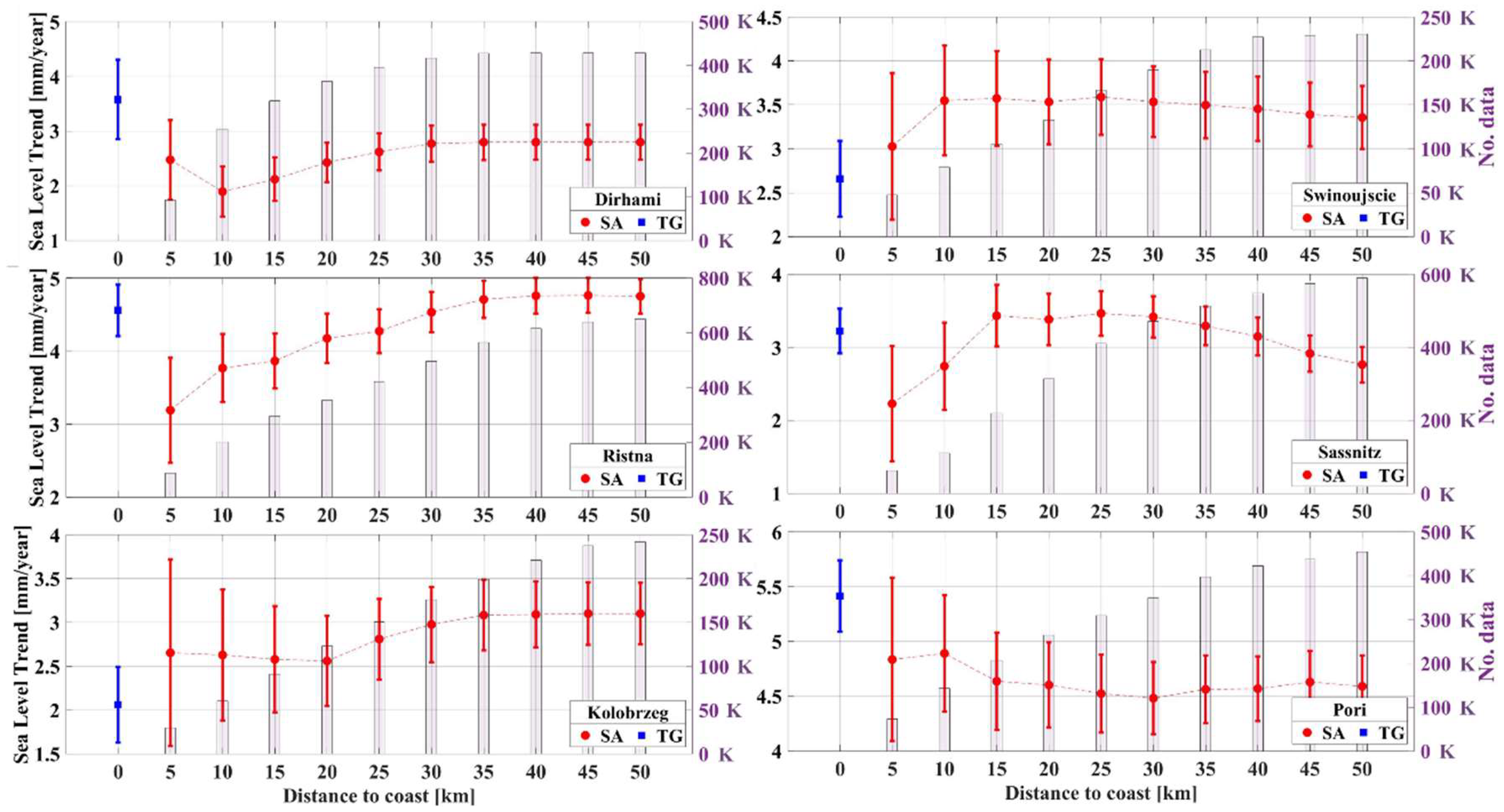
5.4.1. SA Data Optimality Regarding the Distance to TG

The utilization of along-track SA data provides an opportunity to investigate how sea-level trend estimates change regarding the distance from the coastline. Figure 10 and

Table 6. Absolute difference [mm/yr] between TG-derived and SA-derived trends at different distances (Dist) from the coast. The values are highlighted based on colour (i.e., the smallest absolute difference is in green and the largest is in red). The corresponding RMSE and arithmetic average (MEAN) of differences are computed at the bottom of the table [mm/yr].

	Dist [km]	5	10	15	20	25	30	35	40	45	50
TG
1		1.1	1.7	1.4	1.1	0.9	0.8	0.8	0.8	0.8	0.8
2		1.4	0.9	0.8	0.5	0.4	0.1	0.1	0.1	0.1	0.1
3		2.9	3.3	3.1	3.2	3.4	3.4	3.5	3.5	3.5	3.4
4		1.7	1.7	1.8	1.7	1.6	1.6	1.6	1.6	1.6	1.7
5		0.6	0.6	0.5	0.5	0.7	0.9	1.0	1.0	1.0	1.0
6		0.4	0.9	0.9	0.9	0.9	0.9	0.8	0.8	0.7	0.7
7		1.0	0.5	0.2	0.2	0.2	0.2	0.1	0.1	0.3	0.5
8		2.8	2.9	2.7	2.6	2.6	2.5	2.5	2.5	2.5	2.5
9		0.2	0.1	0.2	0.4	0.5	0.5	0.6	0.5	0.5	0.5
10		1.1	1.1	1.0	0.6	0.3	0.2	0.3	0.6	0.7	0.7
11		0.5	1.1	0.7	0.5	0.4	0.4	0.4	0.4	0.3	0.3
12		1.8	2.1	2.1	2.1	2.0	1.9	1.9	1.9	1.9	1.9
13		0.6	0.5	0.8	0.8	0.9	0.9	0.9	0.8	0.8	0.8
RMSE		1.49	1.63	1.53	1.47	1.48	1.46	1.48	1.48	1.48	1.47
MEAN		0.28	0.16	0.11	0.03	−0.06	−0.12	−0.13	−0.09	−0.08	−0.06

present the SA-derived sea-level trend results, which range from 5 to 50 km away from the coast. In Figure 10, the data within each distance range are averaged, such as averaging the SA data from 5 to 20 km away from the TG station to determine the SA sea-level trend within that distance. Additionally, the TG-derived trend is depicted for comparison, providing insight into the expected sea level at the coast. This comparison aims to illustrate the variability in sea-level trends away from the TG station and potentially explore scenarios where the TG might not consistently offer the optimal location for determining precise sea-level trend estimates, depending on the specific purpose.

Figure 10 illustrates the variability in sea level among stations and distances, highlighting that the dynamics observed at a TG station may not consistently represent the broader coastal area. For instance, at stations like Dirhami (#1) and Pori (#13), the TG trends are higher compared to the SA measurements, whereas at stations like Kolobrzeg (#5), they are lower. These variations may be attributed to persistent marine dynamics influencing coastal areas, such as surface waves causing wave set-up and set-down [81]. However, further investigation is required to fully understand and address these discrepancies in future studies. Meanwhile, Table 6 presents station-specific statistics, revealing only slight variations in RMSE across different distances (ranging from 1.47 to 1.63). Consequently, almost any distance within 50 km appears to be suitable. Notably, the largest RMSEs of 1.63 and 1.53 mm/yr are observed within the 10–15 km ranges from the coast. This discrepancy could be attributed to the specific coastal processes occurring within this distance range.

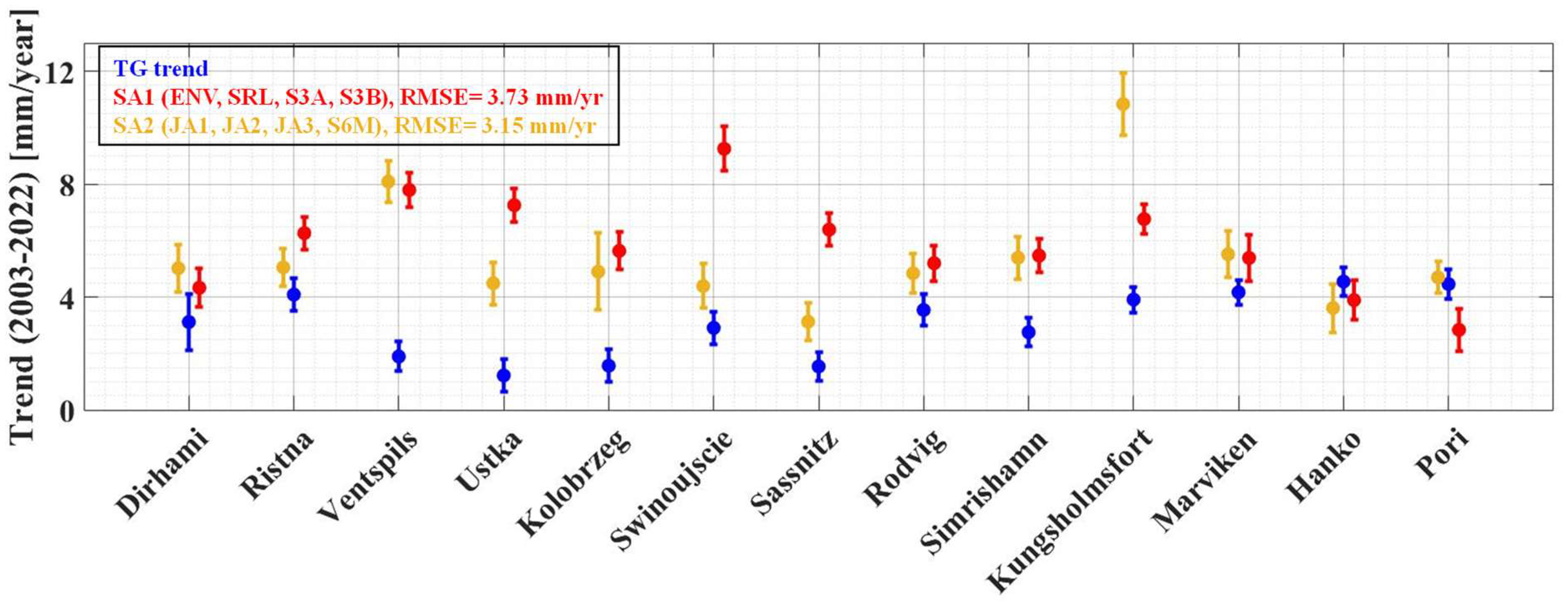
5.4.2. Sea-Level Trends of Different SA Orbit Inclination Categories

As mentioned earlier, the sea-level trend can be estimated by merging multi-mission SA data over different time frames. However, some studies have shown that various SA missions could lead to different data quality depending on their constellation across different regions, which could also affect the subsequent trend estimation. For instance, over sub-arctic areas, low-inclination SA mission orbits (e.g., the Jason series) are able to provide better data than high-inclination orbit missions (e.g., Envisat, Sentinel series, etc.) that align more closely with ground-truth observations [33], although the high-inclination SA missions have better coverage and larger quantities of data [82]. Therefore, in this study, the SA missions were divided into two distinct groups based on their constellation: high-inclination (SA1) and low-inclination (SA2) orbit satellites (cf. Figure 3). This division aimed to investigate whether these distinctions could impact the SA-derived sea-level trend. The sea-level trend of each orbit category was estimated for the period of 2003–2022 (when the overlapped satellite mission data existed) and compared with the ground truth, the hourly TG-derived trend for the same time period (number of measurements is not normalized). These results are illustrated in Figure 11.

The results of the comparison of each SA group with the TG data are represented in

Table 7. Sea-level trend [mm/yr] from TG observation and different orbit inclination categories of SA missions (high- and low-inclination orbit) during 2003–2022 at different stations. Better agreements with the ground truth are denoted in bold font.

ID	Station	TG	SA1	SA2
1	Dirhami	3.12 ± 0.33	4.33 ± 0.23	5.02 ± 0.28
2	Ristna	4.09 ± 0.19	6.26 ± 0.19	5.05 ± 0.22
3	Ventspils	1.89 ± 0.18	7.79 ± 0.20	8.09 ± 0.24
4	Ustka	1.22 ± 0.19	7.25 ± 0.20	4.49 ± 0.25
5	Kolobrzeg	1.57 ± 0.19	5.63 ± 0.22	4.90 ± 0.45
6	Swinoujscie	2.91 ± 0.19	9.25 ± 0.26	4.39 ± 0.26
7	Sassnitz	1.54 ± 0.17	6.39 ± 0.19	3.12 ± 0.22
8	Rodvig	3.54 ± 0.19	5.20 ± 0.21	4.84 ± 0.24
9	Simrishamn	2.75 ± 0.17	5.47 ± 0.20	5.39 ± 0.25
10	Kungsholmsfort	3.91 ± 0.15	6.76 ± 0.18	10.83 ± 0.36
11	Marviken	4.17 ± 0.15	5.39 ± 0.27	5.51 ± 0.28
12	Hanko	4.55 ± 0.17	3.89 ± 0.23	3.61 ± 0.29
13	Pori	4.46 ± 0.18	2.84 ± 0.25	4.70 ± 0.19

(the best match with ground truth is highlighted in bold font). In general, the SA2 group (low inclination) with an RMSE of 3.15 mm/yr had a better match with the TG-derived trend compared to the SA1 group, which has an RMSE of 3.73 mm/yr. Over the 13 stations, the average discrepancy of the SA2 group is 2.5 mm/yr, with a maximum discrepancy of 6.9 mm/yr at Kungsholmsfort (#10), while the average discrepancy between the SA1 group and TG trends is 3.2 mm/yr, with the maximum discrepancy of 6.3 mm/yr at Swinoujscie (#6). However, for some stations, both SA groups have large discrepancies, including Ventspils (#3) and Ustka (#4), which could be due to the TG estimation problems, as is also shown in Figure 7b,c.

5.4.3. Gridded vs. Instantaneous SA-Derived ASL Trends

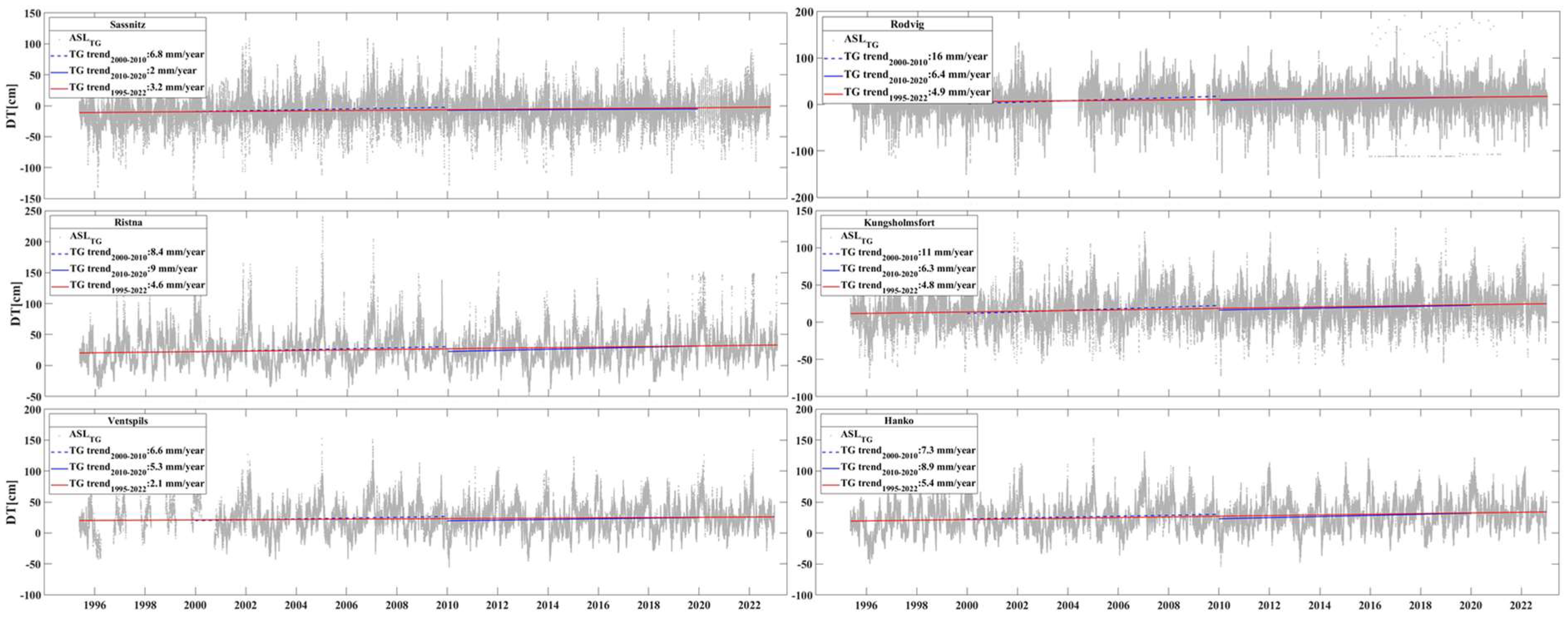
Gridded SA data are frequently utilized for sea-level trend estimations ([29,45,46,83]; etc.). Gridded data are quite convenient, as they average data from various missions, bridging temporal gaps between them and allowing for mutual usage with other data products. This study has focused on using along-track data for sea-level trend estimates. The results have shown that, for the long-term sea-level trends, the SA-based estimates perform reasonably well when compared with hourly TG-derived trends, yielding RMSEs that vary between 1.2 and 1.5 mm/yr. Recall that the long-term (1995–2022) TG sea-level trends varied from 2.1 to 5.4 mm/yr and the along-track SA was 2.5 to 5.3 mm/yr (see Section 5.1 and Table 6). These results are more or less comparable with other studies that have also shown long-term trend estimates of 3.4 mm/yr [45] and 3 mm/yr [29].

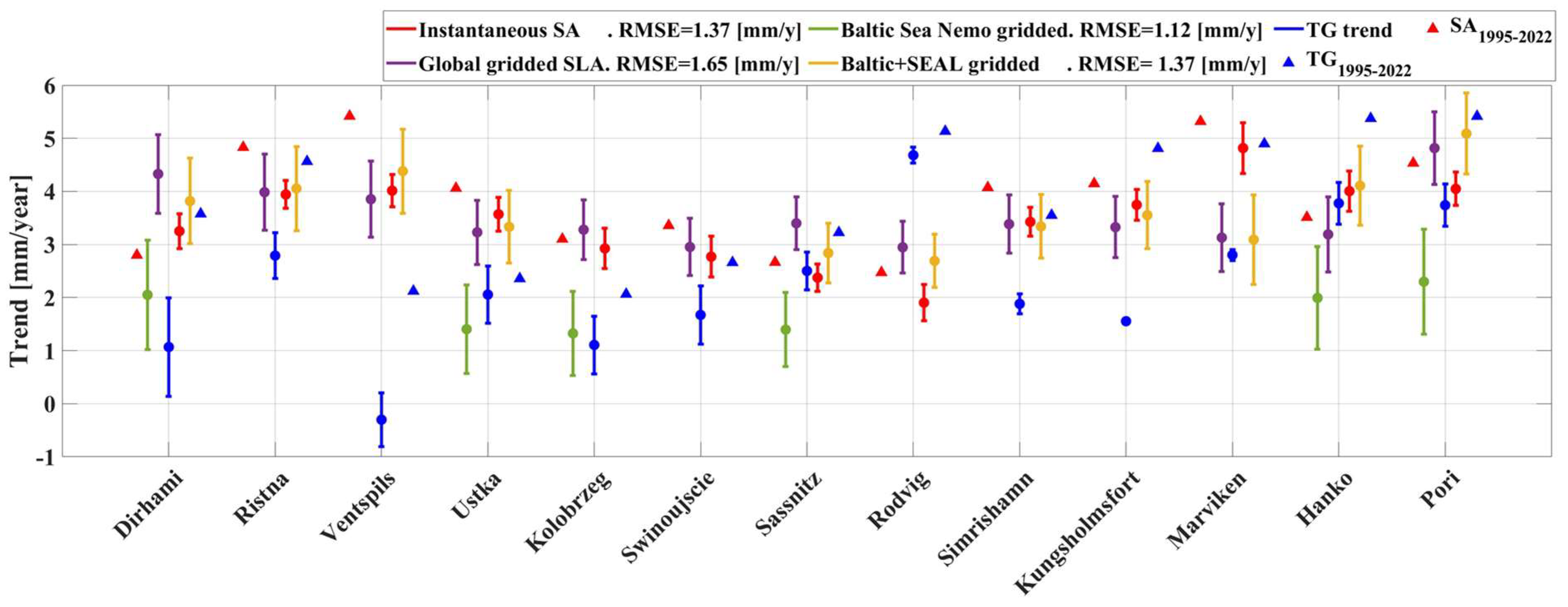
In practice, gridded SA data employ averaging methods and various techniques in processing, which could potentially result in the misinterpretation of sea-level trends. This effect might be more pronounced in coastal areas, impacting their approach and analysis. Moreover, it is also shown in Section 5.4.2 that different SA missions may give different results, whereas this can vary spatially. Regional sea-level trend estimation using SA is more challenging compared to the utilization of SA products for global-scale studies. It is expected that the Baltic Sea area, which has numerous archipelagos, small islands, and rocks within ~10 km of the mainland, may contaminate the radar signal, making less opportunities for SA beams to interact with the open water and leading to errors [29,33,82]. The question now remains as to whether utilizing the SA along-track instantaneous data for sea-level trend research is advantageous over other gridded products. Consequently, this study performs a comparison of sea-level trends from instantaneous along-track SA data with that of three available gridded datasets within this region. These three gridded datasets consist of (i) a global SA gridded sea-level anomaly, (ii) hydrodynamic model gridded products obtained from Nemo (Baltic Sea Physical Reanalysis), and (iii) Baltic + SEAL gridded SA data over the Baltic Sea region obtained from the Baltic + SEAL dataset. More detailed information on these data sources can be found in Section 4.5.

This examination amongst the different sea-level products is performed from 1995 to 2019 (the upper limit is due to the availability of the Baltic + SEAL project data for along-track and gridded data being available only up to June 2019, cf. Table 2). The result of this comparison is shown in Figure 12. The results of the inter-comparison show that most of the gridded products agreed well with the instantaneous SA-derived trend calculations in the present study. In Figure 12, the long-term (28 years) trend variations (the results of Figure 7 and Table 5) from TGs (${DT}_{TG}$) and SA (${DT}_{SA@TG}$) are also illustrated (triangle marker) for comparison. The largest TG trend differences appear to occur with the Baltic+SEAL gridded data, with a difference of 4.7 mm/yr at the Ventspils (#3) station, as well as with the global gridded SLA for Dirhami (#1) of 3.3 mm/yr. The TG data at Ventspils (#3) and Rodvig (#8) also showed somewhat larger differences compared to the other products. Possible reasons are discussed in Section 5.3.

Figure 12 shows that, in general, the instantaneous SA-derived ASL trend results match those of the gridded datasets. Note that the gridded SA data of the Copernicus dataset could not come close enough to the coastline to estimate the sea-level trend for seven TG stations. Hence, the RMSE is compared only for the six available stations. Although the instantaneous SA and gridded data from Baltic + SEAL have the same RMSE, the gridded data also could not come close to the two TG stations’ (Kolobrzeg and Swinoujscie) estimate. This emphasizes the advantage of using the instantaneous SA-derived DT rather than gridded and SLA data for realistic sea-level trend calculations.

Table 8. Sea-level trend estimates [mm/yr] during 1995–2019 using hourly TG observations, instantaneous SA-derived DT, and three gridded data products (incl. global gridded SLA, Baltic Sea Nemo gridded data, and Baltic + SEAL gridded data). The best performances compared to TG observations are in bold font. The ASL trend of TG and SA during 1995–2022 (from Figure 7 and Table 6) is also mentioned. The shape in parenthesis corresponds to the shapes in Figure 12.

ID	TG (●) 1995–2019	SA (●) 1995–2019	Global SLA (●) 1995–2019	Nemo (●) 1995–2019	SEAL (●) 1995–2019	TG (▲) 1995–2022	SA (▲) 1995–2022
1	1.07 ± 0.31	3.25 ± 0.11	4.33 ± 0.0	2.05 ± 0.0	3.82 ± 0.03	3.6 ± 0.02	2.8 ± 0.01
2	2.79 ± 0.14	3.94 ± 0.09	3.98 ± 0.0	NaN	4.05 ± 0.03	4.6 ± 0.01	4.8 ± 0.01
3	−0.3 ± 0.17	4.01 ± 0.10	3.85 ± 0.0	NaN	4.38 ± 0.03	2.1 ± 0.01	5.4 ± 0.01
4	2.06 ± 0.18	3.57 ± 0.11	3.23 ± 0.0	1.40 ± 0.0	3.33 ± 0.02	2.4 ± 0.01	4.1 ± 0.01
5	1.11 ± 0.18	2.92 ± 0.13	3.28 ± 0.0	1.33 ± 0.0	NaN	2.1 ± 0.01	3.1 ± 0.01
6	1.67 ± 0.18	2.77 ± 0.13	2.95 ± 0.0	NaN	NaN	2.7 ± 0.01	3.4 ± 0.01
7	2.50 ± 0.12	2.37 ± 0.09	3.40 ± 0.0	1.40 ± 0.0	2.84 ± 0.02	3.2 ± 0.01	2.7 ± 0.01
8	4.68 ± 0.05	1.90 ± 0.11	2.95 ± 0.0	NaN	2.69 ± 0.02	5.1 ± 0.01	2.5 ± 0.01
9	1.88 ± 0.06	3.43 ± 0.09	3.38 ± 0.0	NaN	3.34 ± 0.02	3.5 ± 0.01	4.1 ± 0.01
10	1.55 ± 0.01	3.75 ± 0.10	3.33 ± 0.0	NaN	3.55 ± 0.02	4.8 ± 0.01	4.1 ± 0.01
11	2.80 ± 0.03	4.82 ± 0.16	3.13 ± 0.0	1.85 ± 0.0	3.09 ± 0.03	4.9 ± 0.01	5.3 ± 0.01
12	3.78 ± 0.13	4.00 ± 0.13	3.19 ± 0.0	1.99 ± 0.0	4.11 ± 0.02	5.4 ± 0.01	3.5 ± 0.01
13	3.74 ± 0.13	4.05 ± 0.10	4.82 ± 0.0	2.30 ± 0.0	5.09 ± 0.03	5.4 ± 0.01	4.5 ± 0.01
RMSE between TG (blue circle and triangle) and SA (red circle and triangle) pairs						1.78	0.64

also includes the long-term trend (28 years) estimations of both SA and TG (the results from Figure 7 and Table 5). From this table, the instantaneous SA-derived trend has a better match with TG (bold fonts) for five stations (Ristna, Swinoujscie, Sassnitz, Hanko, and Pori) as compared to other datasets. These results show that the instantaneous along-track data are comparable to those of the gridded SA products, in which SA appears to work better for regional trend estimation over this area at several TG stations. This could be due to averaging the instantaneous DT within 50 km rather than taking one observation (of TG) for trend computation. In Table 8, the RMSE values are calculated between the pair (${DT}_{TG}$ and ${DT}_{SA@TG}$) of long-term (28 years) and 1995–2019 (24 years) trends of 1.78 mm/yr (blue circles and blue triangles) and 0.64 mm/yr (red circle and red triangles), respectively. In Figure 12, the RMSE between ${DT}_{TG}$ (blue circles) and other datasets over the same period (1995–2019) is also mentioned (stations with any NaN value are excluded). The RMSE between the ${DT}_{TG}$ trend (blue circles) and the ${DT}_{SA@TG}$ trend (red circles) is 1.37 mm/yr. The RMSE between ${DT}_{TG}$ and the Baltic+SEAL gridded data (yellow circles) is 1.37 mm/yr, that of the Nemo gridded data (green circles) is 1.12, and for the global gridded SLA data (purple circles), this is 1.65 mm/yr. The RMSE values also approve the reliability of SA data for trend estimations, which has an insignificant effect on the 4-year difference in the time series.

6. Discussion

In this study, an analysis was conducted on sea-level trends covering a long-term period (28 years, from 1995 to 2022) as well as decadal scales (2000–2009 and 2010–2020) with the focus mainly on the Baltic Proper within the Baltic Sea region. The dataset utilized included information from 13 TG stations along with multi-mission along-track SA. Below is a summary of the key findings.

To begin, on average, the long-term ASL trend calculated for the entire Baltic across the period 1995–2022 revealed consistent results: on average, 3.83 (cf. Table 5) mm/yr for TG hourly data, 3.87 mm/yr for instantaneous SA data, and 3.32 mm/yr for TG at the time of the SA pass (as indicated in Table 5). Notably, all three calculation methods demonstrated relatively similar outcomes. These findings align with prior studies over the same study area: [45] reported trend estimates of 3.4 mm/yr, [29] indicated 3 mm/yr, and [46] achieved comparable results for different time periods using SA, TG, and hydrodynamic models. When compared to the global mean sea level (GMSL) trends obtained from TG and SA data, which exhibited rates ranging from 3.2 mm/yr over the period 1993–2015 to 3.6 mm/yr over the period 2006–2015 [5], the long-term sea-level trend calculated for the Baltic Sea appeared consistent. Importantly, this trend seemed unaffected by the considered time span or the specific data source examined.

This study also explored the long-term RSL and ASL derived from TG hourly data spanning 1995–2022. The findings indicate the significance of accounting for VLM in accurately quantifying trend rates (Section 5.1). For instance, in this analysis, the RSL trends ranged from −2 to 4.5 mm/yr, while the ASL trends varied between 2 and 5.4 mm/yr. Notably, given the spatial variability of VLM rates, the most substantial disparities between the RSL and ASL were observed in locations significantly affected by pronounced VLM. Consequently, in the northern and eastern regions of the Baltic Sea, a distinct pattern emerged, where the ASL displayed an increasing trend from south to north, while the RSL exhibited a decreasing trend from north to south, as evidenced, for instance, at the Pori station (#13). This discrepancy highlights the impact of VLM on sea-level measurements in these specific areas. Moreover, the ASL trend derived from satellite altimetry (SA) data can be effectively compared to the RSL trend derived from TG data. This comparison serves the purpose of either refining or validating the models designed to account for VLM.

The analysis revealed a spatial variation in sea-level trends within the Baltic Sea region, indicating larger values (ranging from 4 to 5 mm/yr) in the north-eastern section compared to stations situated in the south-west (between 2 and 4 mm/yr). Previous studies, such as by [63], suggested that this discrepancy could be attributed to an escalation in the frequency and intensity of westerly winds. Additionally, an increase in cyclones occurring above 52°N has exposed the Baltic Sea to more vigorous westerly storms, potentially contributing to these observed trends. Supporting these findings, a recent report by [84] noted a general pattern of rising water temperatures, a reduced ice extent, and an overall uptick in annual mean precipitation across the northern region. Specifically, in the northern Baltic Sea and the Gulf of Finland, there is a statistical association between larger river runoff and warmer air temperatures coupled with increased precipitation. Conversely, in more southerly regions, a decline in annual runoff corresponds with rising air temperatures. These observations collectively support the notion of varied influences impacting sea-level trends across different sections of the Baltic Sea.

The long-term trends consistently highlight larger rates in the northern section, aligning with findings from earlier studies. Interestingly, these results reveal an anomaly in certain south-western stations, specifically at Rodvig (#8) and Kungsholmsfort (#10), where higher-than-normal trends of approximately 5.1 mm/yr and 4.8 mm/yr, respectively, were calculated using TG hourly data. These rates notably exceed the trends observed at other south-western stations, which typically range within 2 to 4 mm/yr. These unexpected findings require further investigations for a deeper understanding of the main drivers behind this. Understanding the main drivers behind these discrepancies is crucial for a comprehensive and accurate interpretation of sea-level trends in these specific south-western stations.

Examining sea-level trend values at decadal scales revealed notable circumstances. During the period from 2000–2009, a majority of stations (9 out of 13) exhibited an increase in sea-level trends compared to the subsequent decade, 2010–2019. While some stations might have been affected by data gaps during this period (Table 4), others remained unaffected. The larger trends observed could potentially be attributed to increased westerly winds, augmented precipitation, and fluctuations in air pressure, as suggested in studies such as by Reißmann et al. (2009) and Gräwe et al. (2019). Further exploration of the possible reasons for these decadal variations may be necessary. Also, it should be noted that the calculated decadal trends diverge significantly from the long-term trend (1995–2022), showcasing variations that nearly triple in some stations. Furthermore, each decade displayed its unique pattern of variation, as outlined in Table 5. These results demonstrate that the interpretation of decadal trends can be more complex, with many more variations existing for several different reasons.

In this study, the inter-comparison of multi-SA missions with different orbit constellations showed that low-inclination satellites appear to give slightly better results for the trend estimation across the studied sites in the Baltic Sea for the period of nineteen years of overlapped data (2003–2022). Also, the superiority of instantaneous SA-derived DT for the sea-level trend estimates, rather than gridded SLA datasets, is illustrated in Figure 12. Although the gridded data product results are comparable to TG and along-track SA data, they may suffer from issues of replicating data close to the coast, and this made the trend estimation unavailable for some stations. So, in conclusion, the along-track data are better for representing the coastal sea-level trends. By comparing the results of Figure 12 and Table 8, which include the trend value during 1995–2022 (triangles) and 1995–2019 (circles), the trend derived from averaging instantaneous SA appears to have better performance than TG observations (lower RMSE value between these years). This could be due to averaging the SA-derived DT within the specific radius (50 km) of the TG station. The TG-derived trend is more sensitive to the time-series length, and changing the time window of TG data could affect the trend estimations in larger values. This was also shown by comparing the ${DT}_{TG@SA cycle}$ and ${DT}_{SA@TG}$ trends over a decadal time frame.

Also, TGs are located at the coast, so they may also be influenced by other processes, such as wave set-up and set-down [81], which may not always be captured by the SA. This may suggest that TG may not be the ideal dataset to represent sea-level variation, especially with trend estimates. However, the ability to precisely compare the variability in sea level between TG and along-track SA at various distances from the coast provides a valuable insight into ocean dynamics. It also highlights that in areas without the presence of TGs, along-track SA can offer an alternative that may yield even more accurate results. As a result, the utilization of the high-resolution geoid for SA to determine DT, coupled with geoid-referenced TG data, enabled a realistic quantification of these differences. Future research could further examine the comparison of TG and along-track SA in coastal areas and the possible identification of coastal processes.

7. Conclusions

This examination of coastal sea-level trends, calculated using tide gauges (TGs) and multi-mission along-track satellite altimetry (SA) for the period 1995–2022, showed that the average absolute sea-level trend for TG and along-track SA varies between 3.32 and 3.86 mm/yr. This agrees with previous regional Baltic Sea studies, with average values of 3 mm/yr, and that of the global mean sea level (GMSL) rate from TG and SA observations, which showed rates of 3.2 mm/yr over the period 1993–2015 to 3.6 mm/yr over the period 2006–2015. A spatial distribution of larger sea-level trends was observed in the northern and eastern areas of the Baltic Sea, and this may be due to increased days of intense westerly winds, lower air pressure, and increased sea temperature. Decadal sea-level trends showed quite a variation in rates, and a possible increase may have occurred in the decade 2000–2009. This study demonstrates that along-track instantaneous SA data can be reasonably utilized for sea-level trend estimates, and that they give a very good alternative for areas where TGs may not be present and for areas that may be influenced by gaps in TG data.

References

- Hooijer, A.; Vernimmen, R. Global LiDAR land elevation data reveal greatest sea-level rise vulnerability in the tropics. Nat. Commun. 2021, 12, 3592. [Google Scholar] [CrossRef]
- Dangendorf, S.; Hay, C.; Calafat, F.M.; Marcos, M.; Piecuch, C.G.; Berk, K.; Jensen, J. Persistent acceleration in global sea-level rise since the 1960s. Nat. Clim. Change 2019, 9, 705–710. [Google Scholar] [CrossRef]
- Church, J.A.; White, N.J. Sea-level rise from the late 19th to the early 21st century. Surv. Geophys. 2011, 32, 585–602. [Google Scholar] [CrossRef]
- Church, J.A.; White, N.J.; Konikow, L.F.; Domingues, C.M.; Cogley, J.G.; Rignot, E.; Gregory, J.M.; van den Broeke, M.R.; Monaghan, A.J.; Velicogna, I. Revisiting the Earth’s sea-level and energy budgets from 1961 to 2008. Geophys. Res. Lett. 2011, 38, 4066. [Google Scholar] [CrossRef]
- Oppenheimer, M.; Glavovic, B.; Hinkel, J.; Van de Wal, R.; Magnan, A.K.; Abd-Elgawad, A.; Cai, R.; Cifuentes-Jara, M.; Deconto, R.M.; Ghosh, T.; et al. Sea Level Rise and Implications for Low Lying Islands, Coasts and Communities. In The Ocean and Cryosphere in a Changing Climate; Cambridge University Press: Cambridge, UK, 2019. [Google Scholar] [CrossRef]
- Abdalla, S.; Kolahchi, A.A.; Ablain, M.; Adusumilli, S.; Bhowmick, S.A.; Alou-Font, E.; Amarouche, L.; Andersen, O.B.; Antich, H.; Aouf, L.; et al. Altimetry for the future: Building on 25 years of progress. Adv. Space Res. 2021, 68, 319–363. [Google Scholar] [CrossRef]
- Pytharouli, S.; Chaikalis, S.; Stiros, S.C. Uncertainty and bias in electronic tide-gauge records: Evidence from collocated sensors. Measurement 2018, 125, 496–508. [Google Scholar] [CrossRef]
- Slangen, A.B.; Church, J.A.; Agosta, C.; Fettweis, X.; Marzeion, B.; Richter, K. Anthropogenic forcing dominates global mean sea-level rise since 1970. Nat. Clim. Change 2016, 6, 701–705. [Google Scholar] [CrossRef]
- Marzeion, B.; Cogley, J.G.; Richter, K.; Parkes, D. Attribution of global glacier mass loss to anthropogenic and natural causes. Science 2014, 345, 919–921. [Google Scholar] [CrossRef] [PubMed]
- Prandi, P.; Meyssignac, B.; Ablain, M.; Spada, G.; Ribes, A.; Benveniste, J. Local Sea level trends, accelerations, and uncertainties over 1993–2019. Sci. Data 2021, 8, 1. [Google Scholar] [CrossRef] [PubMed]
- Ablain, M.; Cazenave, A.; Valladeau, G.; Guinehut, S. A new assessment of the error budget of global mean sea level rate estimated by satellite altimetry over 1993–2008. Ocean. Sci. 2009, 5, 193–201. [Google Scholar] [CrossRef]
- Ablain, M.; Cazenave, A.; Larnicol, G.; Balmaseda, M.; Cipollini, P.; Faugère, Y.; Fernandes, M.J.; Henry, O.; Johannessen, J.A.; Knudsen, P.; et al. Improved sea level record over the satellite altimetry era (1993–2010) from the Climate Change Initiative project. Ocean Sci. 2015, 11, 67–82. [Google Scholar] [CrossRef]
- Ablain, M.; Meyssignac, B.; Zawadzki, L.; Jugier, R.; Ribes, A.; Spada, G.; Benveniste, J.; Cazenave, A.; Picot, N. Uncertainty in satellite estimates of global mean sea-level changes, trend and acceleration. Earth Syst. Sci. Data 2019, 11, 1189–1202. [Google Scholar] [CrossRef]
- Watson, C.S.; White, N.J.; Church, J.A.; King, M.A.; Burgette, R.J.; Legresy, B. Unabated global mean sea-level rise over the satellite altimeter era. Nat. Clim. Change 2015, 5, 565–568. [Google Scholar] [CrossRef]
- Guérou, A.; Meyssignac, B.; Prandi, P.; Ablain, M.; Ribes, A.; Bignalet-Cazalet, F. Current observed global mean sea level rise and acceleration estimated from satellite altimetry and the associated measurement uncertainty. Ocean Sci. 2023, 19, 431–451. [Google Scholar] [CrossRef]
- Wöppelmann, G.; Letetrel, C.; Santamaria, A.; Bouin, M.N.; Collilieux, X.; Altamimi, Z.; Williams, S.D.P.; Miguez, B.M. Rates of sea-level change over the past century in a geocentric reference frame. Geophys. Res. Lett. 2009, 36, L12607. [Google Scholar] [CrossRef]
- Jevrejeva, S.; Moore, J.C.; Grinsted, A.; Woodworth, P.L. Recent global sea level acceleration started over 200 years ago? Geophys. Res. Lett. 2008, 35. [Google Scholar] [CrossRef]
- Cazenave, A.; Dieng, H.B.; Meyssignac, B.; Von Schuckmann, K.; Decharme, B.; Berthier, E. The rate of sea-level rise. Nat. Clim. Change 2014, 4, 358–361. [Google Scholar] [CrossRef]
- Ablain, M.; Legeais, J.F.; Prandi, P.; Marcos, M.; Fenoglio-Marc, L.; Dieng, H.B.; Benveniste, J.; Cazenave, A. Satellite Altimetry-based Sea Level at Global and Regional Scales. In Integrative Study of the Mean Sea Level and Its Components; Springer International Publishing: Cham, Switzerland, 2017; pp. 9–33. [Google Scholar] [CrossRef]
- Chen, X.; Zhang, X.; Church, J.A.; Watson, C.S.; King, M.A.; Monselesan, D.; Legresy, B.; Harig, C. The increasing rate of global mean sea-level rise during 1993–2014. Nat. Clim Change 2017, 7, 492–495. [Google Scholar] [CrossRef]
- Hay, C.C.; Morrow, E.; Kopp, R.E.; Mitrovica, J.X. Probabilistic reanalysis of twentieth-century sea-level rise. Nature 2015, 517, 481–484. [Google Scholar] [CrossRef] [PubMed]
- Legeais, J.F.; Ablain, M.; Zawadzki, L.; Zuo, H.; Johannessen, J.A.; Scharffenberg, M.G.; Fenoglio-Marc, L.; Fernandes, M.J.; Andersen, O.B.; Rudenko, S.; et al. An improved and homogeneous altimeter sea level record from the ESA Climate Change Initiative. Earth Syst. Sci. Data 2018, 10, 281–301. [Google Scholar] [CrossRef]
- Rateb, A.; Scanlon, B.R. Demystifying the Dynamics of Global and Regional Sea Level Trends from 1993 to 2021. EarthArXiv 2023, X5K38R. [Google Scholar] [CrossRef]
- Simpson, M.J.; Nilsen, J.E.Ø.; Ravndal, O.R.; Breili, K.; Sande, H.; Kierulf, H.P.; Steffen, H.; Jansen, E.; Carson, M.; Vestøl, O. Sea Level Change for Norway: Past and Present Observations and Projections to 2100. Norwegian Centre for Climate Services Report. no. 1/2015. Available online: https://www.researchgate.net/profile/Jan-Even-Nilsen/publication/281626674_Sea_Level_Change_for_Norway_Past_and_Present_Observations_and_Projections_to_2100/links/55f0774708ae199d47c212f6/Sea-Level-Change-for-Norway-Past-and-Present-Observations-and-Projections-to-2100.pdf (accessed on 20 December 2022).
- Slangen, A.B.A.; Carson, M.; Katsman, C.A.; Van de Wal, R.S.W.; Köhl, A.; Vermeersen, L.L.A.; Stammer, D. Projecting twenty-first century regional sea-level changes. Clim. Change 2014, 124, 317–332. [Google Scholar] [CrossRef]
- Kopp, R.E.; Horton, R.M.; Little, C.M.; Mitrovica, J.X.; Oppenheimer, M.; Rasmussen, D.J.; Strauss, B.H.; Tebaldi, C. Probabilistic 21st and 22nd century sea-level projections at a global network of tide-gauge sites. Earth’s Future 2014, 2, 383–406. [Google Scholar] [CrossRef]
- Grinsted, A.; Jevrejeva, S.; Riva, R.E.; Dahl-Jensen, D. Sea level rise projections for northern Europe under RCP8. 5. Clim. Res. 2015, 64, 15–23. [Google Scholar] [CrossRef]
- Fox-Kemper, B.; Hewitt, H.T.; Xiao, C.; Adalgeirsdóttir, G.; Drijfhout, S.S.; Edwards, T.L.; Golledge, N.R.; Hemer, M.; Kopp, R.E.; Krinner, G.; et al. Ocean, Cryosphere and Sea Level Change. In Climate Change 2021: The Physical Science Basis. Contribution of Working Group I to the Sixth Assessment Report of the Intergovernmental Panel on Climate Change; Masson-Delmotte, V., Zhai, P., Anna, P., Conners, S.L., Péan, C., Berger, S., Caud, N., Chen, Y., Goldfarb, L., Gomis, M.I., et al., Eds.; Cambridge University Press: Cambridge, UK; New York, NY, USA, 2021; pp. 1211–1362. Available online: https://www.ipcc.ch/report/ar6/wg1/downloads/report/IPCC_AR6_WGI_Chapter09.pdf (accessed on 20 December 2022).
- Passaro, M.; Müller, F.L.; Oelsmann, J.; Rautiainen, L.; Dettmering, D.; Hart-Davis, M.G.; Abulaitijiang, A.; Andersen, O.B.; Høyer, J.L.; Madsen, K.S.; et al. Absolute Baltic Sea level trends in the satellite altimetry era: A revisit. Front. Mar. Sci. 2021, 8, 647607. [Google Scholar] [CrossRef]
- Pellikka, H.; Johansson, M.M.; Nordman, M.; Ruosteenoja, K. Probabilistic projections and past trends of sea level rise in Finland. Nat. Hazards Earth Syst. Sci. Discuss. 2022, 2022, 1613–1630. [Google Scholar] [CrossRef]
- IPCC; Pörtner, H.O.; Roberts, D.C.; Masson-Delmotte, V.; Zhai, P.; Tignor, M.; Poloczanska, E.; Weyer, N.M. The Ocean and Cryosphere in a Changing Climate. In IPCC Special Report on the Ocean and Cryosphere in a Changing Climate; Cambridge University Press: Cambridge, UK, 2019; p. 1155. [Google Scholar] [CrossRef]
- IPCC Working Group III: Climate Change 2022 Mitigation of Climate Change. Available online: https://report.ipcc.ch/ar6/wg3/IPCC_AR6_WGIII_Full_Report.pdf (accessed on 20 December 2022).
- Mostafavi, M.; Delpeche-Ellmann, N.; Ellmann, A.; Jahanmard, V. Determination of Accurate Dynamic Topography for the Baltic Sea Using Satellite Altimetry and a Marine Geoid Model. Remote Sens. 2023, 15, 2189. [Google Scholar] [CrossRef]
- Varbla, S.; Ågren, J.; Ellmann, A.; Poutanen, M. Treatment of tide gauge time series and marine GNSS measurements for vertical land motion with relevance to the implementation of the Baltic Sea Chart Datum 2000. Remote Sens. 2022, 14, 920. [Google Scholar] [CrossRef]
- Bingham, R.J.; Knudsen, P.; Andersen, O.; Pail, R. An initial estimate of the North Atlantic steady-state geostrophic circulation from GOCE. Geophys. Res. Lett. 2011, 38. [Google Scholar] [CrossRef]
- Knudsen, P.; Bingham, R.; Andersen, O.; Rio, M.H. Enhanced mean dynamic topography and ocean circulation estimation using GOCE preliminary models. J. Geod. 2011, 85, 861–879. [Google Scholar] [CrossRef]
- Knudsen, P.; Andersen, O.; Maximenko, N. A new ocean mean dynamic topography model, derived from a combination of gravity, altimetry and drifter velocity data. Adv. Space Res. 2021, 68, 1090–1102. [Google Scholar] [CrossRef]
- Dean, R.G.; Houston, J.R. Recent sea level trends and accelerations: Comparison of tide gauge and satellite results. Coast. Eng. 2013, 75, 4–9. [Google Scholar] [CrossRef]
- Räike, A.; Oblomkova, N.; Svendsen, L.M.; Kaspersson, R.; Haapaniemi, J.; Eklund, K.; Brynska, W.; Hytteborn, J.; Tornbjerg, H.; Kotilainen, P.; et al. Background Information on the Baltic Sea Catchment Area for the Sixth Baltic Sea Pollution Load Compilation (PLC-6). 2019. Available online: https://helcom.fi/wp-content/uploads/2020/01/PLC-6-background-report.pdf (accessed on 20 December 2022).
- Ekman, M. Climate changes detected through the world’s longest sea level series. Glob. Planet. Change 1999, 21, 215–224. [Google Scholar] [CrossRef]
- Dailidienė, I.; Davulienė, L.; Tilickis, B.; Stankevičius, A.; Myrberg, K. Sea level variability at the Lithuanian coast of the Baltic Sea. Boreal Environ. Res. 2006, 11, 109–121. [Google Scholar]
- Tervo, M.; Poutanen, M.; Koivula, H. Tide gauge monitoring using GPS. In Proceedings of the Dynamic Planet: Monitoring and Understanding a Dynamic Planet with Geodetic and Oceanographic Tools IAG Symposium, Cairns, Australia, 22–26 August 2005; Springer: Berlin/Heidelberg, Germany, 2007; pp. 75–79. [Google Scholar] [CrossRef]
- Richter, A.; Groh, A.; Dietrich, R. Geodetic observation of sea-level change and crustal deformation in the Baltic Sea region. Phys. Chem. Earth Parts A/B/C 2012, 53, 43–53. [Google Scholar] [CrossRef]
- Lyszkowicz, A.; Bernatowicz, A. Geocentric changes of the mean sea level of the Baltic Sea from altimeter and tide gauge data. In Proceedings of the 2018 Baltic Geodetic Congress (BGC Geomatics), Olsztyn, Poland, 21–23 June 2018; IEEE: New York, NY, USA, 2018; pp. 202–206. [Google Scholar] [CrossRef]
- Madsen, K.S.; Høyer, J.L.; Suursaar, Ü.; She, J.; Knudsen, P. Sea level trends and variability of the Baltic Sea from 2D statistical reconstruction and altimetry. Front. Earth Sci. 2019, 7, 243. [Google Scholar] [CrossRef]
- Kapsi, I.; Kall, T.; Liibusk, A. Sea Level Rise and Future Projections in the Baltic Sea. J. Mar. Sci. Eng. 2023, 11, 1514. [Google Scholar] [CrossRef]
- Pajak, K.; Blaszczak-Bak, W. Baltic sea level changes from satellite altimetry data based on the OptD method. Acta Geodyn. Geomater. 2019, 16, 235–244. [Google Scholar] [CrossRef]
- Couhert, A.; Cerri, L.; Legeais, J.F.; Ablain, M.; Zelensky, N.P.; Haines, B.J.; Lemoine, F.G.; Bertiger, W.I.; Desai, S.D.; Otten, M. Towards the 1 mm/y stability of the radial orbit error at regional scales. Adv. Space Res. 2015, 55, 2–23. [Google Scholar] [CrossRef]
- Ekman, M. Postglacial rebound and sea level phenomena, with special reference to Fennoscandia and the Baltic Sea. Suom. Geodeettisen Laitok. Julk. 1993, 115, 7–70. [Google Scholar]
- Jahanmard, V.; Delpeche-Ellmann, N.; Ellmann, A. Towards realistic dynamic topography from coast to offshore by incorporating hydrodynamic and geoid models. Ocean Model. 2022, 180, 102124. [Google Scholar] [CrossRef]
- Jahanmard, V.; Hordoir, R.; Delpeche-Ellmann, N.; Ellmann, A. Quantification of hydrodynamic model sea level bias utilizing deep learning and synergistic integration of data sources. Ocean Model. 2023, 186, 102286. [Google Scholar] [CrossRef]
- Schwabe, J.; Ågren, J.; Liebsch, G.; Westfeld, P.; Hammarklint, T.; Mononen, J.; Andersen, O.B. The Baltic Sea Chart Datum 2000 (BSCD2000): Implementation of a common reference level in the Baltic Sea. Int. Hydrogr. Rev. 2020, 29, 63–82. [Google Scholar]
- Cazenave, A.; Llovel, W. Contemporary sea level rise. Annu. Rev. Mar. Sci. 2010, 2, 145–173. [Google Scholar] [CrossRef] [PubMed]
- Masters, D.; Nerem, R.S.; Choe, C.; Leuliette, E.; Beckley, B.; White, N.; Ablain, M. Comparison of global mean sea level time series from TOPEX/Poseidon, Jason-1, and Jason-2. Mar. Geod. 2012, 35 (Suppl. 1), 20–41. [Google Scholar] [CrossRef]
- Dieng, H.B.; Cazenave, A.; Von Schuckmann, K.; Ablain, M.; Meyssignac, B. Sea level budget over 2005–2013: Missing contributions and data errors. Ocean Sci. 2015, 11, 789–802. [Google Scholar] [CrossRef]
- Nerem, R.S.; Beckley, B.D.; Fasullo, J.T.; Hamlington, B.D.; Masters, D.; Mitchum, G.T. Climate-change–driven accelerated sea-level rise detected in the altimeter era. Proc. Natl. Acad. Sci. USA 2018, 115, 2022–2025. [Google Scholar] [CrossRef] [PubMed]
- Altman, D.G.; Bland, J.M. Standard deviations and standard errors. bmj 2005, 331, 903. [Google Scholar] [CrossRef] [PubMed]
- Hamlington, B.D.; Chambers, D.P.; Frederikse, T.; Dangendorf, S.; Fournier, S.; Buzzanga, B.; Nerem, R.S. Observation-based trajectory of future sea level for the coastal United States tracks near high-end model projections. Commun. Earth Environ. 2022, 3, 230. [Google Scholar] [CrossRef]
- Chang, J.H.; Lee, W.S. A sliding window method for finding recently frequent itemsets over online data streams. J. Inf. Sci. Eng. 2004, 20, 753–762. [Google Scholar] [CrossRef]
- Ku-Mahamud, K.R.; Zakaria, N.; Katuk, N.; Shbier, M. Third Asia International Conference on Modelling & Simulation. In Proceedings of the 2009 Third Asia International Conference on Modelling & Simulation, Bandung, Indonesia, 25–29 May 2009; IEEE: New York, NY, USA, 2009; pp. 45–50. [Google Scholar] [CrossRef]
- Delpeche-Ellmann, N.; Giudici, A.; Rätsep, M.; Soomere, T. Observations of surface drift and effects induced by wind and surface waves in the Baltic Sea for the period 2011–2018. Estuar. Coast. Shelf Sci. 2021, 249, 107071. [Google Scholar] [CrossRef]
- Rajabi-Kiasari, S.; Delpeche-Ellmann, N.; Ellmann, A. Forecasting of absolute dynamic topography using deep learning algorithm with application to the Baltic Sea. Comput. Geosci. 2023, 178, 105406. [Google Scholar] [CrossRef]
- Gräwe, U.; Klingbeil, K.; Kelln, J.; Dangendorf, S. Decomposing mean sea level rise in a semi-enclosed basin, the Baltic Sea. J. Clim. 2019, 32, 3089–3108. [Google Scholar] [CrossRef]
- Weisse, R.; Dailidienė, I.; Hünicke, B.; Kahma, K.; Madsen, K.; Omstedt, A.; Parnell, K.; Schöne, T.; Soomere, T.; Zhang, W.; et al. Sea level dynamics and coastal erosion in the Baltic Sea region. Earth Syst. Dyn. 2021, 12, 871–898. [Google Scholar] [CrossRef]
- Pindsoo, K.; Soomere, T. Basin-wide variations in trends in water level maxima in the Baltic Sea. Cont. Shelf Res. 2020, 193, 104029. [Google Scholar] [CrossRef]
- Delpeche-Ellmann, N.; Mingelaitė, T.; Soomere, T. Examining Lagrangian surface transport during a coastal upwelling in the Gulf of Finland, Baltic Sea. J. Mar. Syst. 2017, 171, 21–30. [Google Scholar] [CrossRef]
- Jakimavičius, D.; Kriaučiūnienė, J.; Šarauskienė, D. Assessment of wave climate and energy resources in the Baltic Sea nearshore (Lithuanian territorial water). Oceanologia 2018, 60, 207–218. [Google Scholar] [CrossRef]
- Tuomi, L.; Rautiainen, L.; Passaro, M. User Manual Along-Track Data Baltic + SEAL. Project: ESA AO/1-9172/17/I-BG-BALTIC+ BALTIC+ Theme 3 Baltic+ SEAL (Sea Level) Requirements Baseline Document/BG-BALTIC+ SEAL (Sea Level) Category: ESA Express Procurement Plus-EXPRO+ Deliverable: D1.1 Code: TUM_BSEAL_RBD; Baltic SEAL: München, Germany, 2020; Available online: http://balticseal.eu/wp-content/uploads/2020/04/Baltic_SEAL_D1.1_RequirementsBaselineDoc_V3.1-signed.pdf (accessed on 9 October 2023).
- Müller, K. (Ed.) Coastal Research in the Gulf of Bothnia; Springer Science & Business Media: Berlin, Germany, 1982; Volume 45, Available online: https://link.springer.com/book/9789061930983 (accessed on 9 October 2023).
- Bonsdorff, E.; Blomqvist, E.M.; Mattila, J.; Norkko, A. Long-term changes and coastal eutrophication. Examples from the Aland Islands and the Archipelago Sea, northern Baltic Sea. Ocean. Acta 1997, 20, 319–329. [Google Scholar]
- Mäkinen, J.; Ihde, J. The permanent tide in height systems. In Observing Our Changing Earth; Springer: Berlin/Heidelberg, Germany, 2009; pp. 81–87. [Google Scholar] [CrossRef]
- Boucher, C.; Altamimi, Z. Memo: Specifications for Reference Frame Fixing in the Analysis of a EUREF GPS Campaign. Version 2011, 8, 18-05. Available online: http://etrs89.ensg.ign.fr/memo-V8.pdf (accessed on 9 October 2023).
- Barbosa, S.M. Quantile trends in Baltic sea level. Geophys. Res. Lett. 2008, 35, L22704. [Google Scholar] [CrossRef]
- Kollo, K.; Ellmann, A. Geodetic reconciliation of tide gauge network in Estonia. Geophysica 2019, 54, 27–38. Available online: https://www.geophysica.fi/pdf/geophysica_2019_54_1_027_kollo.pdf (accessed on 9 October 2023).
- Vestøl, O.; Ågren, J.; Steffen, H.; Kierulf, H.; Tarasov, L. NKG2016LU: A new land uplift model for Fennoscandia and the Baltic Region. J. Geod. 2019, 93, 1759–1779. [Google Scholar] [CrossRef]
- Ågren, J.; Strykowski, G.; Bilker-Koivula, M.; Omang, O.; Märdla, S.; Forsberg, R.; Ellmann, A.; Oja, T.; Liepins, I.; Parseliunas, E.; et al. The NKG2015 gravimetric geoid model for the Nordic-Baltic region. In Proceedings of the 1st Joint Commission 2 and IGFS Meeting International Symposium on Gravity, Geoid and Height Systems, Thessaloniki, Greece, 19–23 September 2016; pp. 19–23. [Google Scholar]
- Agha Karimi, A.; Bagherbandi, M.; Horemuz, M. Multidecadal sea level variability in the Baltic Sea and its impact on acceleration estimations. Front. Mar. Sci. 2021, 8, 702512. [Google Scholar] [CrossRef]
- Olivieri, M.; Spada, G. Spatial sea-level reconstruction in the Baltic Sea and in the pacific Ocean from tide gauges observations. Ann. Geophys. 2016, 59, P0323. [Google Scholar] [CrossRef]
- Omstedt, A.; Pettersen, C.; Rodhe, J.; Winsor, P. Baltic Sea climate: 200 yr of data on air temperature, sea level variation, ice cover, and atmospheric circulation. Clim. Res. 2004, 25, 205–216. [Google Scholar] [CrossRef]
- Lehmann, A.; Getzlaff, K.; Harlaß, J. Detailed assessment of climate variability in the Baltic Sea area for the period 1958 to 2009. Clim. Res. 2011, 46, 185–196. [Google Scholar] [CrossRef]
- Soomere, T.; Pindsoo, K.; Kudryavtseva, N.; Eelsalu, M. Variability of distributions of wave set-up heights along a shoreline with complicated geometry. Ocean Sci. 2020, 16, 1047–1065. [Google Scholar] [CrossRef]
- Mostafavi, M.; Delpeche-Ellmann, N.; Ellmann, A. Accurate sea surface heights from Sentinel-3A and Jason-3 retrackers by incorporating high-resolution marine geoid and hydrodynamic models. J. Geod. Sci. 2021, 11, 58–74. [Google Scholar] [CrossRef]
- Naeije, M.; Di Bella, A.; Geminale, T.; Visser, P. CryoSat Long-Term Ocean Data Analysis and Validation: Final Words on GOP Baseline-C. Remote Sens. 2023, 15, 5420. [Google Scholar] [CrossRef]
- HELCOM, Climate Change in the Baltic Sea. 2021 Fact Sheet. Baltic Sea Environment Proceedings n°180. HELCOM/Baltic Earth 2021. Available online: https://helcom.fi/post_type_publ/climate-change-in-the-baltic-sea-2021-fact-sheet/ (accessed on 9 October 2023).
Figure 1.
Inter-relations between the participating datasets (TG, and SA), geoid model, and different reference ellipsoids (ΔE) and relevant coordinate systems. The geoid change () and vertical land motion (VLM) at the time instants (t) need to be considered for TG readings according to the reference time epoch (). TGs could refer to different national/pan-continental datums (e.g., ETRF) while SA data refer to different global reference frames (e.g., ITRF). For the rest of the used abbreviations, see the main body of the text.
Figure 2.
Flowchart of the applied method.
Figure 3.
Available satellite altimeter missions are used in this study. The coloured (corresponding to the orbit inclination; ~66°: yellow, ~98°: red, ~92°: green) portion of bars demonstrate the duration (arrow for the presently ongoing missions) of the SA missions. The SA revisit cycles in days (d) are also indicated for each mission in the brackets.
Figure 4.
Spatial distribution of SA data at locations of selected TG stations within the 50 km radius. The white points represent the removed SA data within 5 km distance from the coastline.
Figure 6.
Annual DT variation of TG observations (hourly data) before (black, RSL) and after (blue, ASL) application of the VLM correction for six selected TG stations during 1995–2022. The bars represent the sea-level variations (minimum and maximum) in each year. The dots represent the DT annual average.
Figure 7.
SA- and TG-derived ASL trend estimates for the period 1995 to 2022. (a) Spatial distribution of the SA (red)- and hourly TG (blue)-based trend estimates. (b) Estimated trends using both instantaneous SA (red) and TG hourly data at each station (dark blue) with the corresponding RMSE = 1.5 mm/yr, and (c) -based trend (light blue) compared with instantaneous SA-derived trend (red), with the corresponding RMSE = 1.2 mm/yr. The whiskers in (b,c) represent the estimated trend uncertainties within the 95% confidence error of each dataset. The green line in (a) divides the study area into north-eastern and south-western sections.
Figure 8.
Sea-level trend estimates using hourly TG records (dark blue) and TG data at the time of SA cycles (light blue) for the period of 1995–2022 and the corresponding amount (%) of missing data in each station. The RMSE between the two estimated trends is 1.08 mm/yr. The whiskers represent the estimated trend uncertainties within 95% CI of each dataset. In general, the stations with missing data show larger discrepancies between the and -based trend estimates.
Figure 9.
Decadal sea-level trend using hourly TG records (dark blue) and TG data at the time of SA cycles (light blue) and SA data (red) over (a) the period of 2000–2019, (b) the 2000–2009 decade, and (c) the 2010–2019 decade. The RMSE is computed between two corresponding datasets. The deviation between the estimated trend values (especially during 2000–2009) is due to the data gaps. The whiskers represent uncertainties using 95% CI.
Figure 10.
SA-derived sea-level trend (red) moving away from the coast compared to the TG trend (blue) at six stations. The whiskers represent the uncertainties using 95% CI. The number of initial (non-averaged) SA data points within the distance are denoted in the right-hand-side vertical axis with numbers in thousand (K) format.
Figure 11.
Estimated sea-level trend at the TG locations for two SA orbit inclination (high—red; low—yellow) categories of SA data compared to the TG-derived trend (blue) for the period of 2003–2022. The whiskers represent uncertainties using 95% CI.
Figure 12.
Sea-level trend estimates based on instantaneous SA data (red) and three gridded datasets including global SLA data by Copernicus (purple), gridded Nemo model SLA by Copernicus (green), and Baltic + SEAL gridded SA data (yellow) together with the TG data (blue) in the period of 1995–2019. The whiskers represent uncertainties using 95% CI. The long-term (1995–2022) trend based on (red triangle) and (blue triangle) are added as a reference.