Enhanced Graph Structure Representation for Unsupervised Heterogeneous Change Detection

Abstract

Heterogeneous change detection (CD) is widely applied in various fields such as urban planning, environmental monitoring, and disaster management. It enhances the accuracy and comprehensiveness of surface change monitoring by integrating multi-sensor remote sensing data. Scholars have proposed many graph-based methods to address the issue of incomparable heterogeneous images caused by imaging differences. However, these methods often overlook the influence of changes in vertex status on the graph structure, which limits their ability to represent image structural features. To tackle this problem, this paper presents an unsupervised heterogeneous CD method based on enhanced graph structure representation (EGSR). This method enhances the representation capacity of the graph structure for image structural features by measuring the unchanged probabilities of vertices, thereby making it easier to detect changes in heterogeneous images. Firstly, we construct the graph structure using image superpixels and measure the structural graph differences of heterogeneous images in the same image domain. Then, we calculate the unchanged probability of each vertex in the structural graph and reconstruct the graph structure using this probability. To accurately represent the graph structure, we adopt an iterative framework for enhancing the representation of the graph structure. Finally, at the end of the iteration, the final change map (CM) is obtained by binary segmentation of the graph vertices based on their unchanged probabilities. The effectiveness of this method is validated through experiments on four sets of heterogeneous image datasets and two sets of homogeneous image datasets.

1. Introduction

1.1. Background

Remote sensing image change detection (CD) is an emerging technology attracting attention across various domains including natural resource monitoring [1,2], disaster warning [3,4], and urban planning [5,6]. It enables the detection and analysis of surface changes on Earth through the comparative analysis of remote sensing images captured within the same geographic region over time. As multi-spectral, hyperspectral, and synthetic aperture radar (SAR) satellites alongside other advanced remote sensing platforms continue to proliferate, the diversity of obtainable remote sensing datasets is rapidly expanding [7,8]. This expansion is propelling the advancement of CD techniques. Depending on the characteristics of the remote sensing data employed, CD approaches can be generally categorized into either homogeneous or heterogeneous CD methods.

Homogeneous CD primarily relies on data acquired from identical sensor platforms. However, this approach is often impeded by low-quality and incomplete datasets resulting from factors such as satellites’ technical limitations and environmental conditions. For instance, optical satellite imagery can be impacted by cloud coverage and sunlight.

In contrast, heterogeneous CD integrates multi-source remote sensing datasets, such as combining optical and SAR images, to identify land surface changes. Compared to homogeneous CD, heterogeneous CD demonstrates several advantages: (1) It maximizes the observational strengths of different sensors. For example, optical sensors provide high-resolution surface details in clear skies whereas SARs’ function is unaffected by illumination. (2) Land modifications originate from natural and human causes, exhibiting complex spatio-temporal properties. In light of this complexity, leveraging heterogeneous imagery proves to be an effective approach. (3) With frequent acquisition across wider areas now, heterogeneous CD improves modification monitoring, frequency, and scope.

However, heterogeneous remote sensing datasets contain divergent spatial, spectral, radiometric, and temporal properties, restricting the direct comparison of traditional homogeneous CD algorithms. Therefore, innovative CD approaches tailored to heterogeneous imagery require development. Recently, scholars have increasingly investigated heterogeneous CD techniques, which are categorized based on detection mechanisms into image spatial transformation, image feature space mapping, and similarity measurement.

Image spatial transformation methods establish pixel statistical models between heterogeneous images to translate pixels from one image space to another. This allows for the statistical properties of data acquired by different sensors to become more uniform, thereby providing a more reliable foundation for subsequent CD. Researchers can conduct analyses of statistical relations between images and select unchanged pixels with the prior knowledge or affinity matrices. Homogeneous pixel transformation models are then constructed to realize CD [9,10,11,12,13,14]. Additionally, deep learning approaches have been applied to heterogeneous images, such as conditional adversarial networks (CAN) [15], cycle-consistent generative adversarial networks (CycleGANs) [16,17], commonality autoencoders (CAs) [18], deep sparse residual models (DSRM) [19], deep translation-based change detection networks (DTCDN) [20], hierarchical extreme learning machine (HELM) [21], and code-aligned autoencoders (CAA) [22]. However, these methods necessitate introducing labeled or pseudo-labeled data.

Image feature space mapping methods map heterogeneous data into a shared feature space to represent similar ground objects with approximate features. This is achieved through methods such as deep learning and mapping network (DLM) [23], symmetric convolutional coupling networks (SCCN) [24], approximate symmetrically deep neural networks (ASDNN) [25], deep capsule networks (DCN) [26], deep pyramid feature learning networks (DPFL) [27], two-stage joint feature learning (TSHFL) [28], and log-based transformation feature learning (LTFL) [29]. By mapping to a common feature space, this approach helps enrich image feature expression and weaken differences between heterogeneous images. However, for cases with complex noise interference like SAR images, misdetection remains a problem to a certain degree. Therefore, there is still a need to further improve algorithm robustness against noise.

Similarity measurement methods mainly detect changes by calculating differences in comparable features between heterogeneous images. Such methods generally do not require supervised guidance and have a high degree of automation. They can be mainly divided into methods based on spectral features and structural features. (1) Spectral feature-based methods detect changes by comparing pixel statistical characteristics without laborious training. For instance, the multivariate statistical model (MSM) [30] applies statistics to model multi-modal pixel values, evaluating similarity or change via statistical feature comparisons. The Markov model for multimodal change detection (M3CD) [31] establishes Markov models relating cross-modal pixel relationships to discern changed areas. Meanwhile, the energy-based model (EBM) [32] quantifies similarity or change through energy distributions or difference metrics. Nonetheless, these approaches underutilize spatial information and are susceptible to noise. Methods based on structural features aim to construct structural information for heterogeneous images. The sorted histogram (SH) [33] assesses pixel similarity by sorting image histograms and comparing them. The graph-based fusion (GBF) [34] emphasizes changed areas by fusing graph structural information and identifying the most dissimilar regions in the graph structure. However, both SH and GBF neglect non-local similarities that are important for capturing contextual information. To address this, the non-local patch-based graph (NLPG) [35] and its improved version (INLPG) [36] construct a graph of structural consistency based on non-local similarities between image patches, evaluating changes in heterogeneous images through this graph. In addition, graph-based image regression and Markov random field (GIR-MRF) [37], and sparse-constrained adaptive structure consistency (SCASC) [38] analyze image structures through regression models considering the correlation of image superpixels to determine changes. To further improve detection accuracy, iterative robust graph and Markovian co-segmentation (IRG-McS) [39] optimize the graph structure and measure the change level of images by comparing the graphs and mapped graphs. The structural relationship graph convolutional autoencoder (SRGCAE) [40] extracts change information by learning the differences in structural relationships of heterogeneous images through graph autoencoders. While these methods offer promising results, their accuracy is limited by their graph structure representation capabilities.

1.2. Motivation and Contribution

First, compared to supervised methods, unsupervised methods in heterogeneous CD tasks offer distinct advantages. They operate independently of labeled training samples, autonomously discovering potential change patterns within data. This approach significantly reduces the cost associated with data annotation, proving more economically viable for practical applications. Moreover, unsupervised methods exhibit flexibility by not being bound by specific supervised labels, making them adaptable to a wide array of remote sensing image change scenarios.

Second, despite substantial differences in the imaging characteristics of heterogeneous images, there exist consistent structural features within unchanged regions [35,36]. Encoding these features into respective structure graphs and subsequently measuring the disparities between these graphs facilitates the detection of changes within heterogeneous images. Graph-based methods, unlike those reliant on individual pixels or image patches, offer noteworthy advantages in heterogeneous CD: (1) each vertex within the graph symbolizes an element in the image, enabling an understanding of spatial contextual relationships and the effective capture of intricate change patterns; (2) structure graphs can circumvent imaging differences in heterogeneous images by exploiting and comparing their consistent structural features in unchanged regions, enhancing the precision and robustness of CD.

Third, precise representation of a structure graph proves pivotal in extracting structural features accurately from heterogeneous images. This precision aids in comprehensively describing spatial relationships between vertices within a structure graph, thereby elevating the accuracy of heterogeneous CD. However, prevalent methods fall short in adequately considering the change information of vertices within structure graphs. This limitation impedes the faithful representation of graph structures concerning the consistency of structural features in heterogeneous images. To address this, IRG-McS [39] utilizes hard-threshold segmentation for the change probabilities of vertices in optimizing graph structures. However, this method’s efficacy remains constrained by the accuracy limitations of the threshold segmentation, hindering a precise measurement of the impact of changed vertices on the structure graph.

In this paper, we propose an enhanced graph structure representation (EGSR) for unsupervised heterogeneous CD. Initially, we construct a structure graph by utilizing superpixels extracted from heterogeneous images as vertices. This method involves comparing the Laplacian matrices of structure graphs derived from various heterogeneous images to quantify their structural dissimilarities, thereby addressing imaging variations among heterogeneous images. Concurrently, we analyze how changes in vertices impact the representation of the graph structure. Unlike traditional methods employing hard-threshold segmentation on vertices, EGSR computes the unchanged probabilities of vertices based on structural differences within heterogeneous images. This strategy facilitates a more refined establishment of connections between vertices. To augment the representation of graph structures further, we introduce an iterative framework that refines vertices’ connections based on the unchanged probabilities of vertices, enhancing the precision of CD. Ultimately, we perform binary segmentation based on structural dissimilarities to generate a change map (CM). The primary contributions of this work include:

(1)

Proposing an unsupervised heterogeneous CD method that measures disparities between heterogeneous images via structural mapping, without necessitating labeled or pseudo-labeled samples. This will enhance the algorithm’s automation, reduce the cost of the algorithm, and improve its adaptability to different change scenarios.

(2)

Introducing a new method to measure structural differences based on the Laplacian matrix, focusing on quantifying connectivity differences between graph vertices for enhanced precision in capturing structural changes in heterogeneous images.

(3)

Enhancing the graph’s representation by considering the unchanged probabilities of vertices and employing an iterative computation framework. The enhanced graph structure is particularly beneficial for improving the capability of CD. The results from four heterogeneous image datasets and two homogeneous image datasets validate the efficacy of the proposed method.

The rest of the paper is organized as follows: Section 2 introduces the proposed method in detail. Section 3 displays the experiments and results. Section 4 discusses the proposed method. Section 5 provides the conclusion and future work.

2. Proposed and Methods

A set of co-registered heterogeneous remote sensing images, $\dot{X}\in {ℝ}^{M\times N\times B_X}$ and $\dot{Y}\in {ℝ}^{M\times N\times B_Y}$, are provided. Where $M$, $N$, and $B_X\left(B_Y\right)$, respectively, represent the length, width, and number of bands of images $\dot{X}\left(\dot{Y}\right)$. The pixels of these images are denoted as $x\left(m,n,b\right)$ and $y\left(m,n,b\right)$, respectively. As images $\dot{X}$ and $\dot{Y}$ belong to different imaging modalities, their spectral features cannot be directly compared. However, in unchanged regions, consistent structure features are demonstrated by images $\dot{X}$ and $\dot{Y}$. By encoding the structural features of images $\dot{X}$ and $\dot{Y}$ into structure graphs, the spatial relationships between images can be better comprehended. Consequently, in this paper, a structural graph is developed to represent the structure features of images $\dot{X}$ and $\dot{Y}$. Measurements of the structural differences between images $\dot{X}$ and $\dot{Y}$ are then facilitated to extract change information from the heterogeneous images.

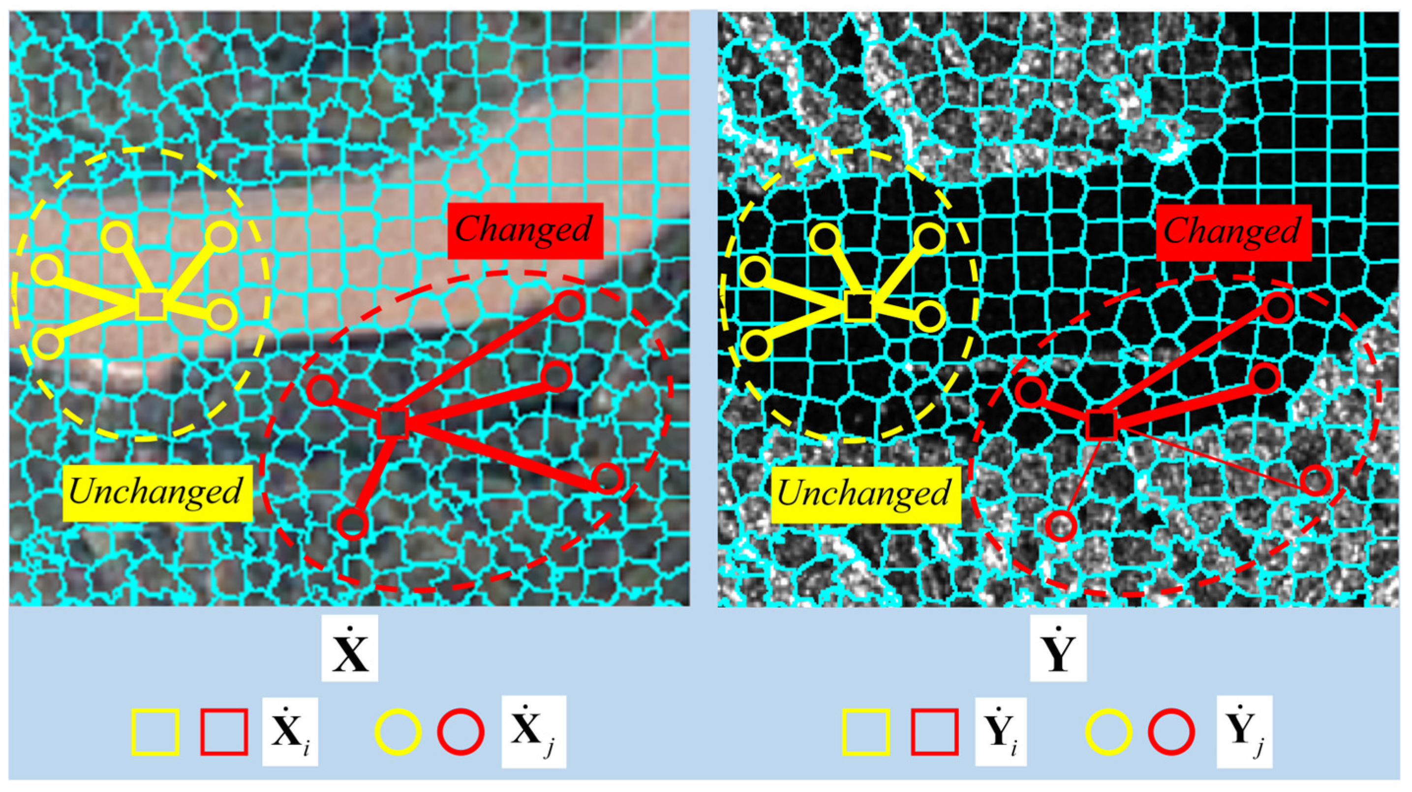
Structural graphs depict the connection relationships between image vertices and their neighbors, reflecting structural features. Changes in image regions induce connection changes between neighboring vertices. To construct structural graphs, each superpixel is treated as an independent vertex representing diverse regions composed of color, texture, etc. The vertices’ relationships reveal patterns and layout of the images. The structural graphs $G_X$ and $G_Y$ of images $\dot{X}$ and $\dot{Y}$ are compared in order to quantify the changes between them. Figure 1 illustrates structural comparison of changed and unchanged areas, exemplifying consistency between ${\dot{X}}_i-{\dot{X}}_j$ and ${\dot{Y}}_i-{\dot{Y}}_j$ connections in unchanged areas and implying unchanged structural features. However, some ${\dot{X}}_i-{\dot{X}}_j$ and ${\dot{Y}}_i-{\dot{Y}}_j$ connections vary in changed areas, agreeing with real changes.

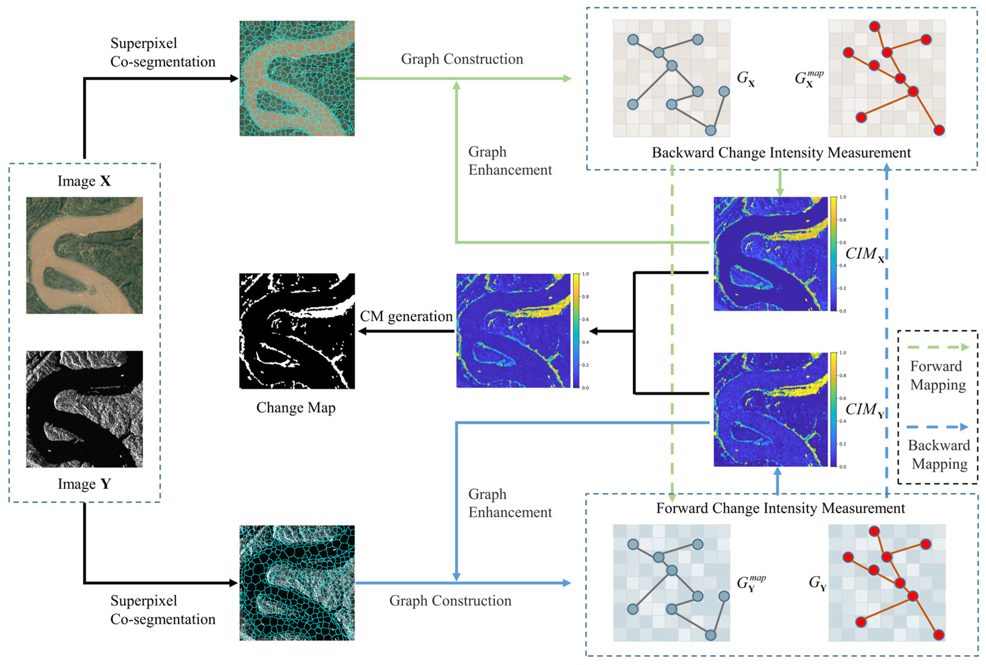
Comparing structural features of heterogeneous images centers around two key aspects: constructing structural features and measuring structural differences. To fulfill this goal, the main content of the proposed EGSR outlined in this paper, as depicted in Figure 2, includes four steps: (1) superpixel co-segmentation of heterogeneous images; (2) structural graph construction and change intensity (CI) measurement; (3) graph structure representation enhancement; (4) CM generation.

2.1. Superpixel Co-Segmentation of Heterogeneous Images

This paper uses superpixels as the basic units for image processing. Superpixels are generated through clustering pixels into uniformly segmented regions, which better preserves structural information compared to traditional image patches or individual pixels. By representing the images as superpixels, discontinuities and noise caused by independent pixel/patch processing can be avoided. Additionally, superpixels help reduce the amount of data processing since fewer superpixel units contain more image information than numerous individual pixels, significantly improving computational efficiency.

In this paper, we use the simple liner iterative clustering (SLIC) [41] algorithm for image superpixel segmentation. The SLIC algorithm segments the image into superpixels based on local color similarity and spatial continuity, exhibiting excellent performance in processing complex scenes while precisely preserving superpixel boundaries. To ensure that images $\dot{X}$ and $\dot{Y}$ have identical superpixel boundaries for building comparable structural features, we first overlay images $\dot{X}$ and $\dot{Y}$. Then, the SLIC algorithm is applied to perform superpixel segmentation on the overlaid images, obtaining a superpixel map $S=\left\{S_i|i=1,2,\dots ,N_S\right\}$. Subsequently, the superpixel map $S=\left\{S_i|i=1,2,\dots ,N_S\right\}$ is mapped back to the individual images $\dot{X}$ and $\dot{Y}$ to derive their respective superpixel sets $\dot{X}=\left\{{\dot{X}}_i|i=1,2,\dots ,N_S\right\}$ and $\dot{Y}=\left\{{\dot{Y}}_i|i=1,2,\dots ,N_S\right\}$, which contain $N_S$ superpixels. To represent the spectral and texture characteristics of each superpixel, its internal mean, median, and variance are extracted as features. This produces the superpixel feature matrices $X\in {ℝ}^{N_S\times 3B_X}$ and $Y\in {ℝ}^{N_S\times 3B_Y}$.

2.2. Structural Graph Construction and CI Measurement

(1) Structural graph construction. Since structural graphs can effectively express image structural feature, we constructed undirected graphs to extract these features. Taking the construction of the structural graph $G_X$ in image $\dot{X}$ as an example, we define $G_X=\left\{V_X,E_X\right\}$ as follows:

$$\begin{array}{l}{V}_X=\left\{{\dot{X}}_i|i=1,2,\dots ,N_S\right\}\\ E_X=\left\{\left({\dot{X}}_i,{\dot{X}}_j\right)|i=1,2,\dots ,N_S,j\in {\Omega }_{X_i},j\ne i\right\}\end{array}$$

(1)

where $V_X$ and $E_X$, respectively, represent the vertices and edges of graph $G_X$, and ${\Omega }_{X_i}$ denotes the index set of neighbors ${\dot{X}}_j$ connected to the vertex ${\dot{X}}_i$.

To describe vertices interconnections in graph $G_X$ more conveniently, we introduce the adjacency matrix $A^X\in {ℝ}^{N_S\times N_S}$:

$$A_{i,j}^X=\left\{\begin{array}{ll}1,& \left({\dot{X}}_i,{\dot{X}}_j\right)\in E_X\\ 0,& \left({\dot{X}}_i,{\dot{X}}_j\right)\notin E_X\end{array}\right.$$

(2)

To better understand the connectivity strength of each vertex, we introduce the degree matrix $D^X$ for the graph $G_X$. The degree matrix $D^X$ plays a crucial role in analyzing the degree distribution of the graph (i.e., the frequency of vertex occurrences), revealing the degree of vertex aggregation and importance. It is a diagonal matrix, where $D_{i,i}^X={\displaystyle {\sum }_j^{N_S}{A}_{i,j}^X}\in {ℝ}^{N_S\times N_S}$. In a similar manner, structural graph $G_Y$ of image $\dot{Y}$ can be constructed.

The number of neighbors $K_i$ for each vertex ${\dot{X}}_i$ is important, as it impacts the ability of the graph to capture structural information. If $K_i$ is too small, the graph may become overly sensitive to noise in the image. Conversely, if $K_i$ is too large, irrelevant neighbors may be introduced, both of which reduce structural expressiveness. Similar to [38], we determine $K_i$ for each vertex ${\dot{X}}_i$ through the following steps: ① We define the maximum and minimum possible neighbor counts as $k_{\max }=⌊k_{ratio}\times N_S⌋$ and $k_{\min }=⌊k_{\max }/10⌋$, where $k_{ratio}$ is the neighbor ratio and $⌊·⌋$ represents floor division. Then, we calculate the feature distance $dis{t}_{i,j}^X={‖X_i-X_j‖}_2^2$ between vertex ${\dot{X}}_i$ and its neighbors, finding the nearest $k_{\max }$ neighbors of ${\dot{X}}_i$. ② We calculate the number of edges $D_{i,i}^X$ associated with each vertex ${\dot{X}}_i$. ③ The number of neighbors $K_i$ is set as $\min \left\{k_{\max },\max \left\{D_{i,i}^X,k_{\min }\right\}\right\}$.

(2) CI Measurement. As previously discussed, analyzing the structural differences in heterogeneous graphs allows us to quantify the CI between heterogeneous images. Consistency in the connectivity of vertices between graphs $G_X$ and $G_Y$ indicates no change between images $\dot{X}$ and $\dot{Y}$. Consequently, measuring the disparities in vertices connectivity within $G_X$ and $G_Y$ is sufficient to compute the CI between images $\dot{X}$ and $\dot{Y}$. To illustrate, considering backward change measurement, the backward CI $di{f}^X$ can be calculated as follows:

$$di{f}_i^X={\displaystyle \sum _{j=1}^{N_S}{‖\left(\left(D_{i,j}^X-A_{i,j}^X\right)-\left(D_{i,j}^Y-A_{i,j}^Y\right)\right)X_j‖}_2^2}$$

(3)

As both $L^X=D^X-A^X$ and $L^Y=D^Y-A^Y$ represent the Laplacian matrices of graphs $G_X$ and $G_Y$, the above equation can be simplified as follows:

$$di{f}_i^X={\displaystyle \sum _{j=1}^{N_S}{‖\left(L_{i,j}^X-L_{i,j}^Y\right)X_j‖}_2^2}$$

(4)

Since graph data are susceptible to the influence of uneven vertex distribution, it is necessary to normalize the Laplacian matrix [42]. The normalization calculation of the Laplacian matrix is as follows: $\tilde{L}=I-D^{-1/2}A{D}^{-1/2}$. Here, $\tilde{L}$ represents the normalized Laplacian matrix, and $I$ is the identity matrix. The normalization of the Laplacian matrix has three main advantages: ① Achieving scaling balance through normalization is crucial, given the potential significant variation in vertex degrees within the original Laplacian matrix. This variation can lead to a disproportionate impact from vertices with higher degrees during analysis. ② Normalization not only reduces numerical errors but also enhances computational stability and accuracy, contributing to improved overall numerical stability. ③ By adapting to different degree distribution characteristics, such as uniform and power-law distributions, normalization enables the algorithm to perform effectively across various scenarios. Therefore, Equation (4) can be rewritten as follows:

$$di{f}_i^X={\displaystyle \sum _{j=1}^{N_S}{‖\left({\tilde{L}}_{i,j}^X-{\tilde{L}}_{i,j}^Y\right)X_j‖}_2^2}$$

(5)

where, ${\tilde{L}}^X$ and ${\tilde{L}}^Y$ are the normalized Laplacian matrices of $L^X$ and $L^Y$, respectively.

Similarly, we can calculate the forward CI $di{f}^Y$:

$$di{f}_i^Y={\displaystyle \sum _{j=1}^{N_S}{‖\left({\tilde{L}}_{i,j}^X-{\tilde{L}}_{i,j}^Y\right)Y_j‖}_2^2}$$

(6)

2.3. Graph Structure Representation Enhancement

In Equation (5), it is crucial to consider the change status of vertices in the graph for accurately calculating structural differences. Changed vertices can confound information with differences in structural features, leading to a reduction in precision for CI measurement. To address this, we introduce an iterative strategy aimed at enhancing the representational capacity of the graph structure and mitigating the impact of changed vertices on the stability of the graph structure.

Taking graph $G_X$ as an example, the initial backward CI $di{f}^X$ can be obtained by Equation (5). The probability $p_{X_i}^{uc}$ of vertex ${\dot{X}}_i$ remaining unchanged can be inferred through $di{f}^X$. Subsequently, the adjacency matrix $A^X$ will be updated according to the probability $p_{X_i}^{uc}$ value to enhance its structural representation capability. In this paper, the fuzzy c-means (FCM) [43] is introduced to calculate the unchanged probability $p_{X_i}^{uc}$. As the uncertainty of vertices states can be effectively addressed by FCM utilizing its fuzzy modeling, it can provide a delicate estimation for unchanged probability $p_{X_i}^{uc}$. Specifically, the objective function optimized by FCM is defined as follows:

$$\begin{array}{l}\min {\displaystyle \sum _{j=1}^C{\displaystyle \sum _{i=1}^{N_S}{u}_{i,j}^m{‖di{f}_i^X-C_j‖}^2}}\\ s.t.{\displaystyle \sum _{j=1}^C{u}_{i,j}}=1,\forall i,j; 0<{\displaystyle \sum _{i=1}^{N_S}{u}_{i,j}}<N_S,\forall j\end{array}$$

(7)

where m is fuzzy factor, typically set to 2 in studies, and represents the degree of classification fuzziness [43]. The membership matrix $U=\left\{u_{i,j}\left|i=1,\dots ,N_S,j=1,\dots ,C\right.\right\}$ indicates the probability of i-th sample belonging to j-th cluster category. The number of clusters $C$ dictates how samples are grouped, with $C_j$ denoting the j-th cluster center. In this study, $C$ is set to 2 to divide $di{f}^X$ into two classes: the unchanged class $C_1$ and changed class $C_2$.

The Lagrange multiplier method is applied to optimize the objective function and update membership degrees through the iterative recalculation of cluster centers. Membership degree $u_{i,j}$ is expressed as follows:

$$u_{i,j}={{\displaystyle \sum _{k=1}^C\left(\frac{{‖di{f}_i^X-C_j‖}^2}{{‖di{f}_i^X-C_k‖}^2}\right)}}^{\frac{1}{1-m}}$$

(8)

When the optimization of the objective function is completed, the probability $p_{X_i}^{uc}$ that each vertex in graph $G_X$ remains unchanged can be calculated as follows:

$$p_{X_i}^{uc}=\left\{\begin{array}{cc}{u}_{i,1},& if di{f}_i^X\in C_1\\ 0,& else\end{array}\right.$$

(9)

Based on the calculated probabilities $p_{X_i}^{uc}$, graph $G_X$ can be optimized through iterative structural enhancements. Suppose the graph undergoes $T$ iterations of refinement, where the graph $G_X$ after the t-th $\left(t=1,2,\dots ,T\right)$ iteration is defined as $G_X^{\left(t\right)}$. The adjacency matrix $A^{X\left(t\right)}$ of graph $G_X^{\left(t\right)}$ is then calculated as follows:

$$A_{\left(i,j\right)}^{X\left(t\right)}=A_{\left(i,j\right)}^{X\left(t-1\right)}+p_{X_i}^{uc\left(t-1\right)}{A}_{\left(i,j\right)}^{X\left(t-1\right)}$$

(10)

In the same way, we can obtain the enhanced graph $G_Y^{\left(t\right)}$.

Then, the backward $di{f}_X$ and forward $di{f}_Y$ can be calculated, respectively, as follows:

$$di{f}_i^X={\displaystyle \sum _{j=1}^{N_S}{‖\left({\tilde{L}}_{i,j}^{X\left(t\right)}-{\tilde{L}}_{i,j}^{Y\left(t\right)}\right)X_j‖}_2^2}$$

(11)

$$di{f}_i^Y={\displaystyle \sum _{j=1}^{N_S}{‖\left({\tilde{L}}_{i,j}^{X\left(t\right)}-{\tilde{L}}_{i,j}^{Y\left(t\right)}\right)Y_j‖}_2^2}$$

(12)

where ${\tilde{L}}^{X\left(t\right)}$ and ${\tilde{L}}^{Y\left(t\right)}$ represent the normalized Laplacian matrices of graphs $G_X^{\left(t\right)}$ and $G_Y^{\left(t\right)}$, respectively.

2.4. CM Generation

Once the iterative calculation is completed, we can obtain the final CI of image changes:

$$di{f}^{final}=di{f}^X/mean\left(di{f}^X\right)+di{f}^Y/mean\left(di{f}^Y\right)$$

(13)

The CI map (CIM) is obtained from the following formula:

$$C{I}_{\left(m,n\right)}=di{f}_i^{final} ; \left(m,n\right)\in S_i$$

(14)

The generation of the CM involves the binary segmentation of the CIM. In this study, we utilize the FCM algorithm for the binary segmentation of CIM to obtain the CM. Algorithm 1 summarizes the main workflow of the proposed EGSR.

Algorithm 1. Framework of EGSR

Input: images $\dot{X}$ and $\dot{Y}$, parameters of $N_s,k_{ratio},T$ Preprocessing: Superpixel co-segmentation of heterogeneous images. Structural graph construction. CI measurement. Main iteration loop of EGSR: For t = 1,2, …, T 1. Calculating the unchanged probabilities $p_{X_i}^{uc}$ and $p_{Y_i}^{uc}$ of ${\dot{X}}_i$ and ${\dot{Y}}_i$ with Equations (8) and (9) 2. Constructing enhanced structured graph $G_X^{\left(t\right)}$ and $G_Y^{\left(t\right)}$ with Equation (10). 3. CI measurement: Calculation of forward and backward CIs by Equations (11) and (12). Exit for Output: Compute the binary CM by FCM.

3. Experiments and Results

This section introduces the experimental dataset, the evaluation metrics, briefly describes the comparison methods and the algorithm parameter settings, and shows the experimental results.

3.1. Experiments

3.1.1. Dataset Description

To validate the effectiveness of the proposed EGSR for heterogeneous CD and assess its applicability for homogeneous CD, we conducted experiments using four heterogeneous datasets (datasets #1–#4) and two homogeneous image datasets (dataset #5 and dataset #6, which consisted of optical images and SAR images, respectively). In each heterogeneous image dataset, the spatial resolutions of the two temporal images are different. To facilitate the CD task, we resampled them to the same spatial resolution. These six datasets encompassed images acquired over wide time spans and across different regions, incorporating diverse change scenarios such as urban construction and river expansion. Therefore, these six comprehensive datasets were able to test the robustness and performance of the proposed method. We generated the ground truth through visual interpretation aided by expert knowledge and by referencing high-resolution imagery close in time and space. Detailed information of each dataset is provided in

Table 1. Experimental datasets.

Dataset	Sensor	Size (Pixels)	Date	Location	Event (and Spatial Resolution)
#1	Google Earth/Sentinel-1	600 × 600 × 3(1)	December 1999–November 2017	Chongqing, China	River expansion (10 m)
#2	Pleiades/WorldView2	2000 × 2000 × 3(3)	May 2012–July 2013	Toulouse, France	Urban construction (0.52 m)
#3	Landsat-8/Sentinel-1	3500 × 2000 × 11(3)	January 2017–February 2017	Sutter County, CA, USA	Flooding (≈15 m)
#4	Sentinel-2/Sentinel-1	444 × 571 × 3(1)	April 2017–October 2020	Lake Poyang, China	Lake expansion (10 m)
#5	Zi-Yuan 3	458 × 559 × 3	2014–2016	Wuhan, China	Urban construction (5.8 m)
#6	Sentinel-1	898 × 1500 × 1	November 2017–May 2018	Chongqing, China	River expansion (10 m)

.

3.1.2. Evaluation Criteria

In order to quantitatively evaluate the effectiveness of the proposed EGSR, several evaluation criteria are used, including percentage of overall accuracy (OA), kappa coefficient (KC), and F1–measure (F1). They are calculated separately as follows:

$$\mathrm{OA}=\left(\mathrm{TP}+\mathrm{TN}\right)/\left(\mathrm{TP}+\mathrm{TN}+\mathrm{FP}+\mathrm{FN}\right)$$

(15)

$$\mathrm{KC}=\left(\mathrm{OA}-\mathrm{PRE}\right)/\left(1-\mathrm{PRE}\right)$$

(16)

where

$$\mathrm{PRE}=\left(\left(\mathrm{TP}+\mathrm{FN}\right)\left(\mathrm{TP}+\mathrm{FP}\right)+\left(\mathrm{TN}+\mathrm{FP}\right)\left(\mathrm{TN}+\mathrm{FN}\right)\right)/{\mathrm{N}}^2$$

(17)

$$\mathrm{F}1=\left(2\mathrm{TP}\right)/\left(2\mathrm{TP}+\mathrm{FP}+\mathrm{FN}\right)$$

(18)

N is the total number of pixels, and TP, FP, TN, and FN denote true positives, false positives, true negatives, and false negatives, respectively.

3.1.3. Comparison Methods

To validate the effectiveness of our proposed method, we compare it against several state-of-the-art approaches.

(1)

LTFL [29]: It employs deep learning for extracting high-dimensional features from heterogeneous images. It subsequently utilizes a change classifier trained on these differences to identify regions that have changed.

(2)

INLPG [36]: This method constructs non-local structural features from heterogeneous images and maps these features to the same image domain for a comparative analysis, aiming to emphasize changed regions.

(3)

GBF [34]: By integrating graph structure information, GBF identifies regions with the most dissimilar graph structures, effectively highlighting areas that have changed.

(4)

IRG-McS [39]: This approach explores superpixel-based structural features in heterogeneous images. By employing Markov co-segmentation, it obtains a feature difference map to identify regions that have changed.

(5)

SCASC [38]: It preserves the structural features of the source image, transforms it into the target image domain with sparse constraints, and extracts change information by comparing the source and transformed images.

(6)

SRGCAE [40]: SRGCAE employs a graph convolutional autoencoder to learn the graph structure relationships of heterogeneous images and extracts change information by contrasting these relationships.

(7)

GIR-MRF [37]: GIR-MRF employs an unsupervised image regression approach grounded in the inherent structure consistency of heterogeneous images, integrating global and local constraints through structured graph learning, and improving detection accuracy with a Markov segmentation model.

3.1.4. Experimental Parameter Setting

In this paper, the maximum iteration count T is set to 5, the neighbor ratio $K_{ratio}$ is set to 0.15, and the number of superpixels $N_S$ is set to 12,000. The key parameters for the proposed algorithm are $K_{ratio}$ and $N_S$, and a detailed analysis of these parameters is presented in Section 4.1.

3.2. Results

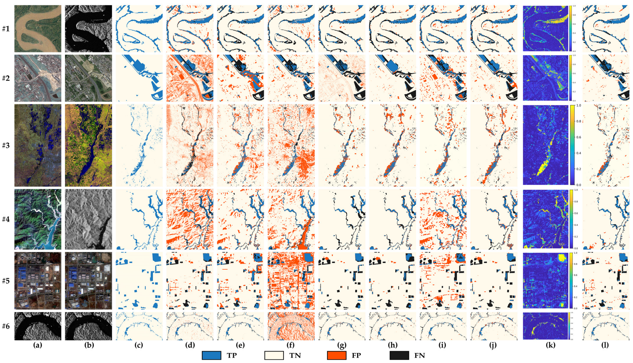
Figure 3 shows the results of CD and the corresponding CIMs generated by the proposed EGSR across datasets #1–6. Dataset #1 poses a challenge with diverse shadow distributions in its land portions. While all the methods successfully pinpoint major changes, LTFL, GBF, and SRGCAE exhibit higher false positives (FPs), whereas IRG-McS, SCASC, and GIR-MRF tend to have more false negatives (FNs). The complexity escalates in dataset #2, introducing intricate change scenarios and increasing FPs for all methods except IRG-McS, SCASC, and GIR-MRF. Notably, SCASC, while boasting fewer FPs, overlooks the change area in the bottom right corner. Dataset #3 reflects changes from flooding disasters, adding difficulty due to complex spectral features. Here, LTFL, INLPG, and GBF misidentify changes on the right side, while IRG-McS, SCASC, SRGCAE, and GIR-MRF accurately identify major changes, with some lingering FPs in the upper part. Transitioning to dataset #4, showcasing river changes, LTFL, INLPG, GBF, and SRGCAE contribute numerous FPs, whereas IRG-McS, SCASC, and GIR-MRF exhibit fewer FPs but more FNs. Moving on, datasets #5 and #6, which are homogeneous image datasets, represent changes in urban areas and rivers, respectively. With the exception of GBF, other comparative methods can more comprehensively detect change areas.

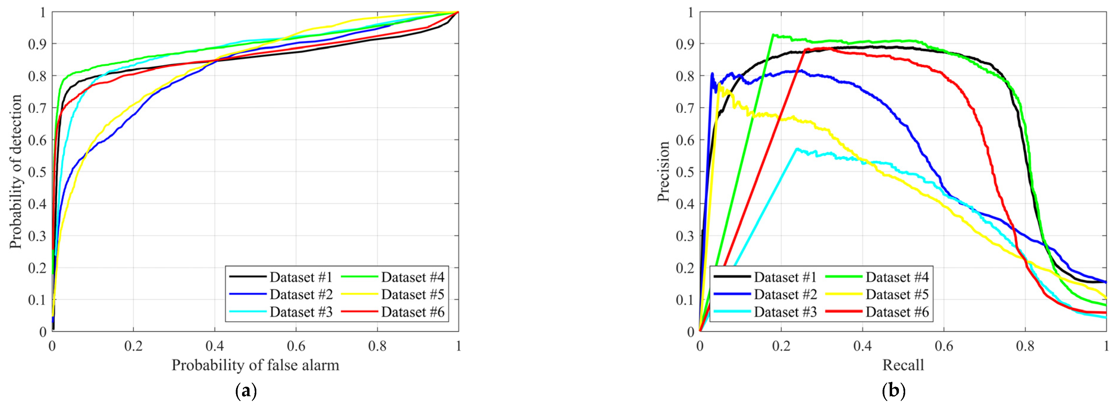
Figure 3k illustrates EGSR effectively highlighting change areas, minimizing both FPs and FNs in its CMs (Figure 3l). To showcase the robustness of the CIMs generated by the proposed EGSR across all datasets, the analysis includes the empirical receiver operating characteristics (ROC) curves and precision–recall (PR) curves. Additionally, corresponding metrics, including the area under the ROC curve (AUR) and the area under the PR curve (AUP), are employed to facilitate a comprehensive evaluation. Figure 4 plots the ROC and PR curves of CIMs generated by the proposed EGSR, and

Table 2. Quantitative measures of CIMs on the datasets #1–#6.

Measures	#1	#2	#3	#4	#5	#6
AUR	0.8545	0.8169	0.8835	0.8965	0.8324	0.8586
AUP	0.7069	0.5497	0.3495	0.6674	0.4354	0.5378

lists the corresponding AUR and AUP. The ROC curves and the PR curves of the proposed EGSR from Figure 4a indicate that conventional threshold segmentation methods can easily distinguish between the changed and unchanged regions in EGSR’s CIMs. This effectiveness arises from EGSR’s ability to enhance the expressiveness of the graph structure through iterative optimization based on changed probabilities of vertices, resulting in a more accurate representation of image structural features and improved identification of changes between heterogeneous images.

Table 3. Quantitative measures of CMs on the heterogeneous datasets #1–#3.

Methods	#1			#2			#3
	OA	KC	F1	OA	KC	F1	OA	KC	F1
LTFL	0.9204	0.7119	0.7579	0.6800	0.2181	0.3862	0.8504	0.0631	0.1240
INLPG	0.9083	0.5635	0.6092	0.8171	0.3395	0.4482	0.9059	0.3730	0.4128
GBF	0.8989	0.5530	0.6109	0.8261	0.2155	0.3105	0.7915	0.1093	0.1737
IRG-McS	0.9128	0.6022	0.6483	0.8685	0.4239	0.4973	0.9469	0.4703	0.4975
SCASC	0.8955	0.5069	0.5599	0.8918	0.4711	0.5247	0.9381	0.4585	0.4888
SRGCAE	0.9223	0.6812	0.7259	0.8231	0.3817	0.4867	0.9376	0.4246	0.4557
GIR-MRF	0.9037	0.5913	0.6457	0.8960	0.4840	0.5350	0.9446	0.4674	0.4954
EGSR	0.9366	0.7329	0.7689	0.8973	0.5029	0.5544	0.9465	0.4784	0.5056

and

Table 4. Quantitative measures of CMs on the heterogeneous datasets #4–#6.

Methods	#4			#5			#6
	OA	KC	F1	OA	KC	F1	OA	KC	F1
LTFL	0.7016	0.1490	0.2600	0.9051	0.4092	0.4598	0.9550	0.6188	0.6428
INLPG	0.9148	0.5426	0.5879	0.8851	0.4500	0.5138	0.9659	0.6448	0.6621
GBF	0.8300	0.3458	0.4231	0.6240	0.1439	0.2845	0.6636	0.1185	0.2087
IRG-McS	0.9450	0.4948	0.5182	0.9203	0.4024	0.4365	0.9591	0.5579	0.5782
SCASC	0.9537	0.6443	0.6684	0.9090	0.3035	0.3407	0.9528	0.4745	0.4974
SRGCAE	0.8354	0.3585	0.4339	0.8354	0.1958	0.2874	0.9592	0.5212	0.5399
GIR-MRF	0.9481	0.6398	0.6678	0.9171	0.3950	0.4321	0.9554	0.5796	0.6031
EGSR	0.9611	0.7072	0.7277	0.9184	0.4673	0.5094	0.9676	0.6594	0.6758

present accuracy metrics for different methods on datasets #1–3 and #4–6. EGSR achieves the highest OA and F1 score on most datasets, with the highest KC across all datasets. Compared to other methods, EGSR improves OA, KC, and F1 values by at least 0.52%, 4.07%, and 2.80%, respectively, demonstrating the effectiveness and robustness of the proposed method.

4. Discussion

4.1. Parameter Analysis

4.1.1. Neighbor Ratio $K_{ratio}$

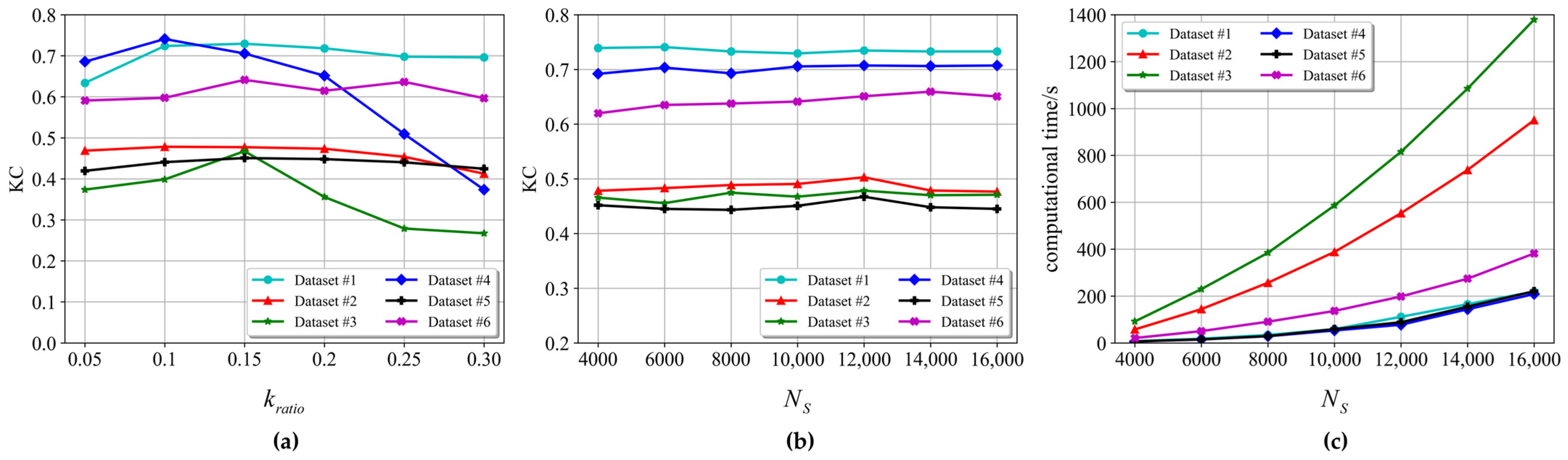
To analyze the impact of the neighbor ratio $k_{ratio}$ on the proposed EGSR, we fix on the number of superpixels $N_S$ at 10,000 and varied $k_{ratio}$ from 0.05 to 0.3 with a step size of 0.05. Figure 5a depicts the accuracy changes in the proposed EGSR corresponding to different $k_{ratio}$ values. The results show that, with the exception of dataset #4, where the KC value of EGSR gradually increases from $k_{ratio}$ 0.05 to 0.1 and then begins to decline, EGSR’s KC value on other datasets generally rises from $k_{ratio}$ 0.05 to 0.15 and then experiences various degrees of decline. This phenomenon is attributed to the fact that selecting too many neighbors can introduce excessive redundancies and inaccuracies, affecting the accuracy of the graph structure. Conversely, too few neighbors may result in an incomplete representation of graph structural features, leading to reduced detection accuracy. It is noteworthy that datasets #3 and #4 capture changes in rivers, encompassing both significant alterations in the main river channels and subtle changes in the tributaries. This necessitates a stringent requirement for the precision of structural feature construction. Consequently, the accuracy of the proposed EGSR declines when $k_{ratio}$ exceeds 0.2, particularly for these two datasets. Nevertheless, the performance of the proposed method remains relatively consistent when $k_{ratio}$ is confined within the range of 0.05 to 0.2. After a thorough analysis and standardization of the parameter settings, this study recommends a universal $k_{ratio}$ value of 0.15 across all datasets.

4.1.2. Number of Superpixels $N_S$

We maintained a neighbor ratio $k_{ratio}$ value of 0.15 while adjusting the number of superpixels $N_S$ within the range of 4000 to 16,000, with a step size of 2000. In Figure 5b, the influence of varying superpixel numbers on the proposed method’s accuracy is depicted. A comparison to the neighbor ratio $k_{ratio}$ reveals that the number of superpixels $N_S$ has a more subtle impact on the accuracy of the proposed EGSR. Across all datasets, the KC value of the proposed EGSR exhibits a slight upward trend within the $N_S$ range of 4000 to 12,000. For datasets #1, #4, and #6, minimal changes in KC values are observed within the $N_S$ range of 12,000 to 16,000, with a slight decrease noted for datasets #1, #4, and #6 in this interval.

In general, a larger number of superpixels $N_S$ enables the detection of finer-grained changes, but this comes at the cost of increased computational time (as shown in Figure 5c) and the potential for excessively fragmented superpixels. Conversely, a smaller number of superpixels may introduce significant internal variances, posing challenges in accurately representing the same physical target and complicating CI measurement. Consequently, this paper establishes the number of superpixels $N_S$ at 12,000.

4.2. Ablation Experiment

4.2.1. The Effectiveness of Iterative Graph Structure Enhancement

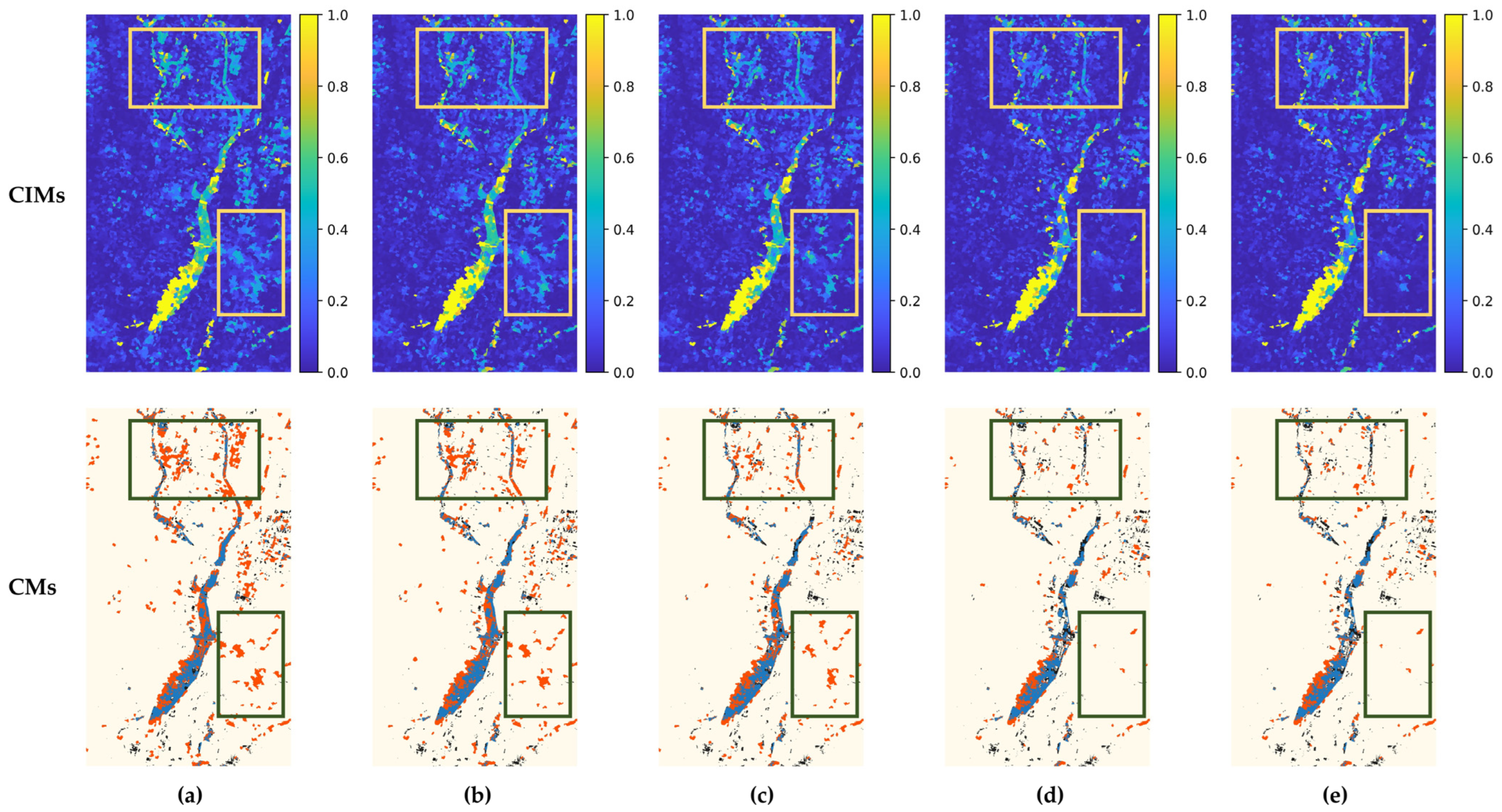
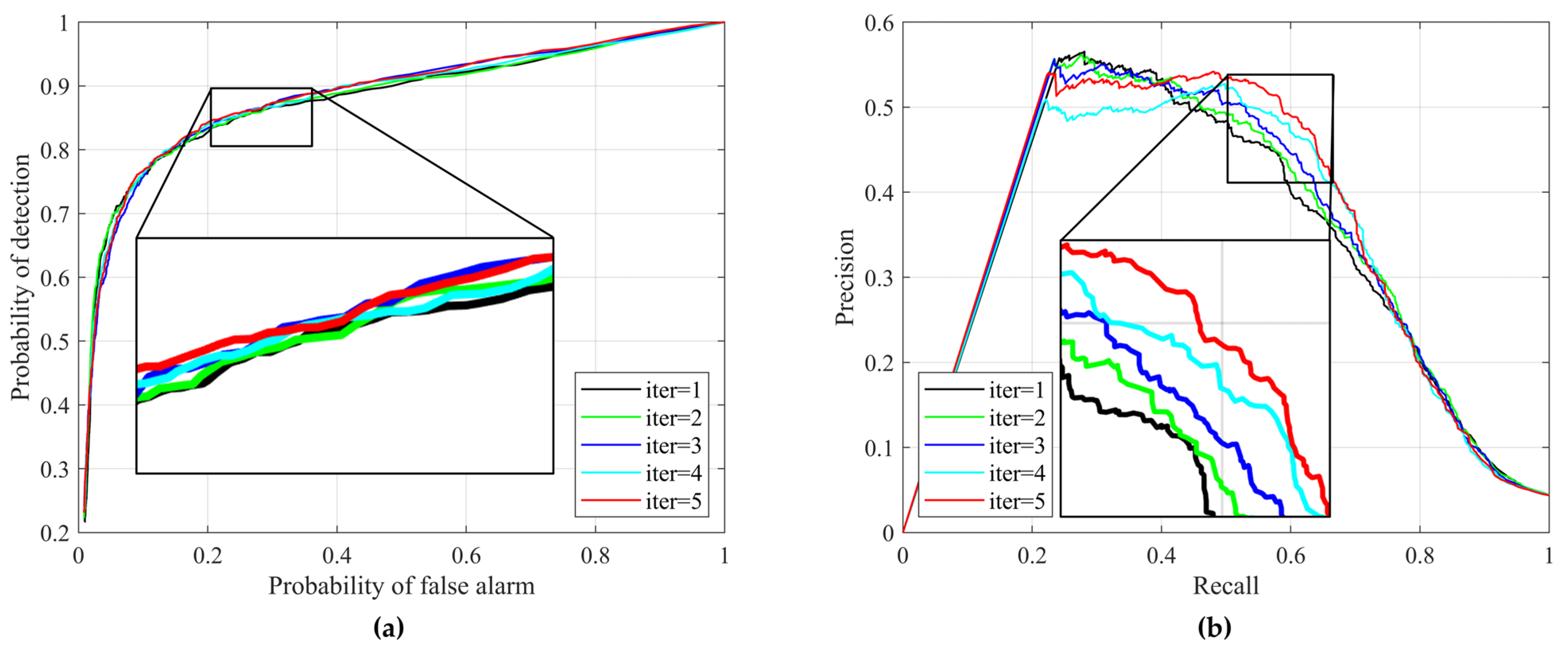
To validate the effectiveness of graph structure enhancement using the proposed method, we analyzed the CIMs and CMs of dataset #3 as the number of iterations increased. Specifically, we examined the first row of Figure 6a–e, which depicted the CIMs, and the second row, which illustrated the CMs. As the iterations progressed, we observed that the contrast between changed and unchanged regions in the CIMs of dataset #3 gradually strengthened, particularly in the boxed areas. Moreover, by inspecting the CMs, we found that the last iteration contained significantly fewer FPs than the initial iteration. To further illustrate the effectiveness of iterative graph structure enhancement, we present the ROC curves and PR curves of EGSR’s CIMs for iterations 1 to 5 (Figure 7). Corresponding AUR and AUP values, as well as relevant metrics for EGSR’s CMs at each iteration, are displayed in

Table 5. Quantitative measures of CIMs and CMs for each iteration of EGSR on dataset #3.

Measures	iter = 1	iter = 2	iter = 3	iter = 4	iter = 5
OA	0.9088	0.9296	0.9412	0.9459	0.9465
KC	0.4339	0.4451	0.4605	0.4787	0.4784
F1	0.4670	0.4943	0.4897	0.5065	0.5056
AUR	0.8769	0.8782	0.8804	0.8817	0.8835
AUP	0.3329	0.3366	0.3394	0.3415	0.3495

. From Figure 7, it is evident that with an increase in the number of iterations, the quality of EGSR’s CIMs gradually improves, making it easier to distinguish between changed and unchanged regions. This demonstrates that graph structure enhancement using the proposed method can accurately characterize the structural features of images by enhancing contrasts, thus improving detection accuracy.

Concurrently, we observe that as the number of iterations increases, the enhancement in the quality of CIMs and CMs generated by EGSR gradually diminishes, as evidenced by the close results of the 4th and 5th iterations. This slowdown in improvement is primarily attributed to the substantial headroom for enhancing graph structure expression ability during the early iterations. However, with the progression of iterations, the enhancement in graph structure representation ability tends to approach its upper limit. Therefore, while augmenting the number of iterations proves beneficial for refining graph structure representation ability, an excessively iterative process becomes resource-consuming. Consequently, we recommend limiting the number of iterations to five, which is deemed sufficient for practical requirements.

4.2.2. The Robustness of EGSR under Different Superpixel Segmentation Methods

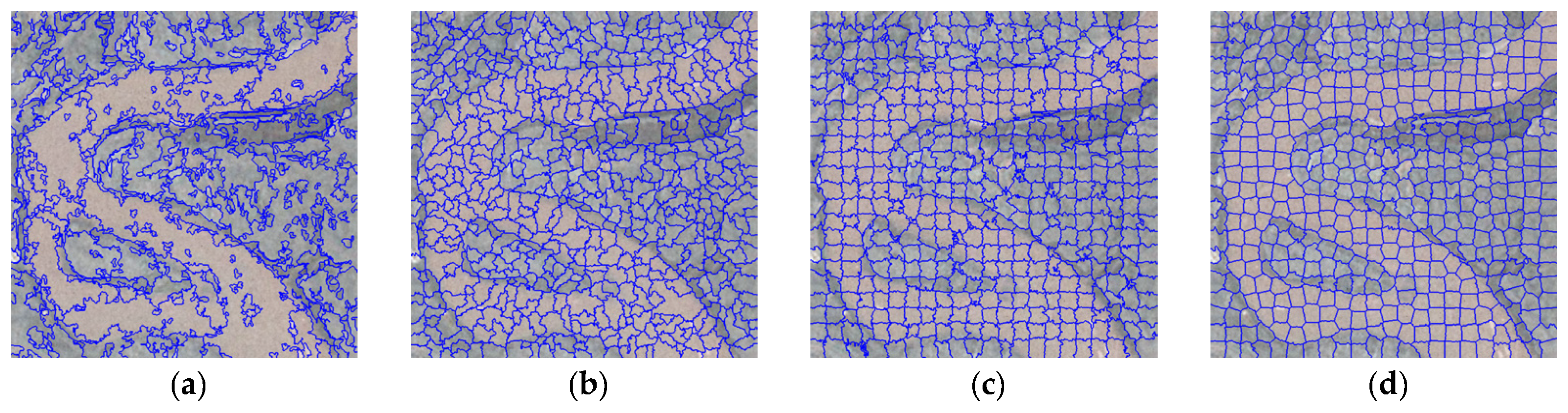
In evaluating the impact of various superpixel segmentation algorithms on our approach, we conducted a comparative analysis using the Felzenszwalb [44], Quickshift [45], and Watershed [46] algorithms. The Felzenszwalb algorithm, which relies on regional features within the image, employs an adaptive edge-merging strategy to generate superpixels of variable sizes. This adaptability renders it suitable for diverse targets with varying scales and shapes. Meanwhile, the Quickshift algorithm, leveraging color and spatial information, identifies superpixel centers through density peaks and gradient information, ensuring rapid superpixel generation. The Watershed algorithm conceptualizes the image as terrain, pinpointing potential watershed points at local minima and segmenting the image by flooding from these points—an approach particularly effective for images with pronounced edge structures. To enhance the illustration of diverse superpixel segmentation effects, we standardized the number of superpixels generated by each algorithm to around 400. The results of the segmentation process for each algorithm on the overlaid image of dataset #1 are depicted in Figure 8.

By observing Figure 8, it becomes evident that the segmentation results exhibit diverse shapes, sizes, and structures, attributed to the distinct core concepts of these superpixel segmentation algorithms. Felzenszwalb and Quickshift prioritize adaptability over the shape and size of the target, Watershed emphasizes the image’s edge structure, and SLIC is distinguished by compact and regular superpixels. Nonetheless, all four superpixel segmentation algorithms demonstrate the capability to generate superpixel regions with uniform spectral and spatial features.

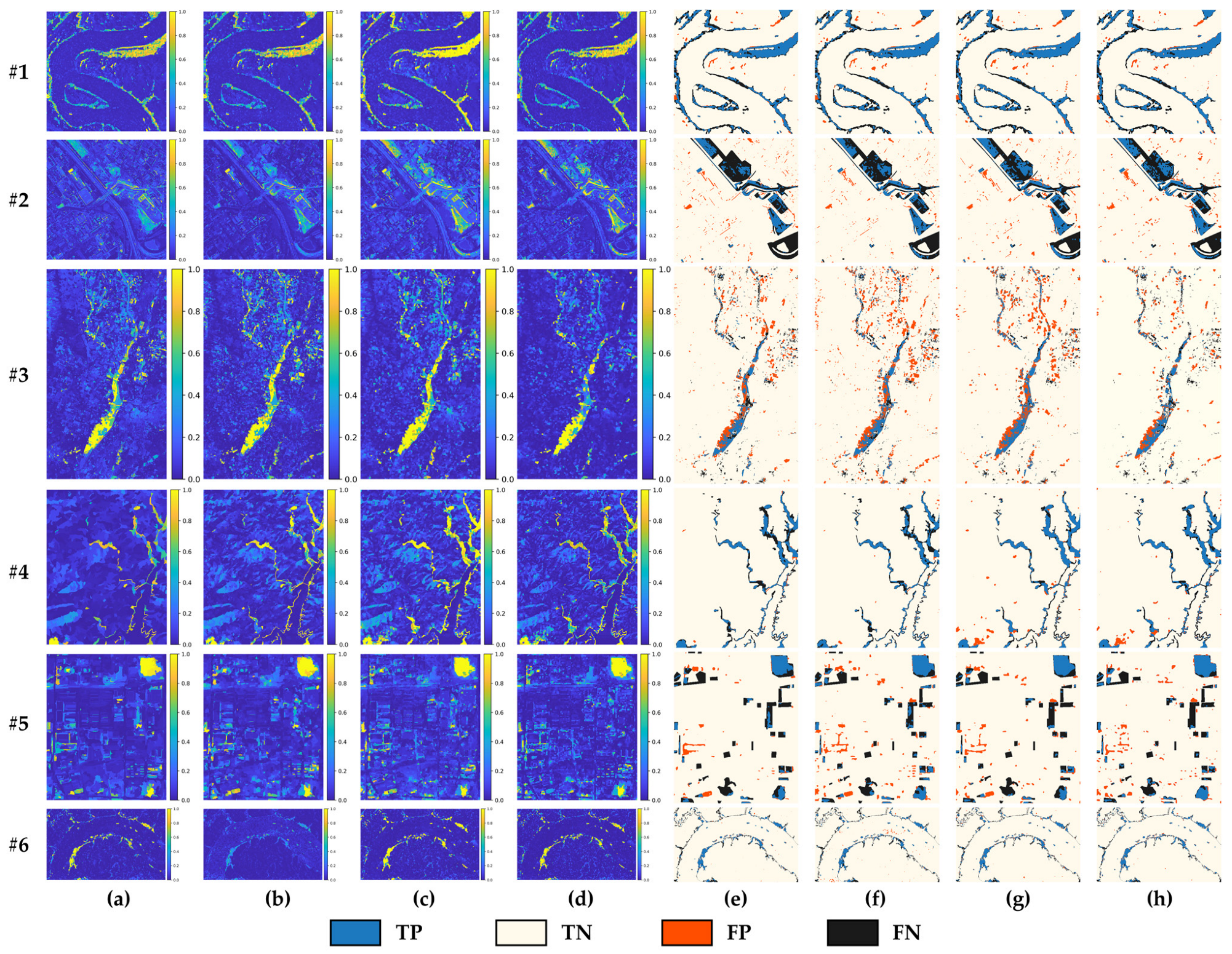
In Figure 9, the results of CIMs and CMs from different superpixel segmentation algorithms on six experimental datasets are presented (the number of superpixels for each method is approximately 12,000). Visually, CIMs produced by the four algorithms significantly highlight changed areas, and CMs accurately extract the edge contours of the changed objects, revealing no apparent differences. For a quantitative assessment and comparison of algorithm performance,

Table 6. Quantitative measures of CMs on the heterogeneous datasets #1–#3.

Methods	Felzenszwalb			Quickshift			Watershed			SLIC
	OA	KC	F1	OA	KC	F1	OA	KC	F1	OA	KC	F1
#1	0.9602	0.7033	0.7243	0.9353	0.7293	0.7662	0.9345	0.7239	0.7610	0.9366	0.7329	0.7689
#2	0.8921	0.4787	0.5331	0.8882	0.4734	0.5317	0.8909	0.4906	0.5480	0.8973	0.5029	0.5544
#3	0.9407	0.4701	0.4994	0.9446	0.4674	0.4954	0.9407	0.4701	0.4994	0.9465	0.4784	0.5056
#4	0.9589	0.6930	0.7147	0.9573	0.6920	0.7149	0.9600	0.7104	0.7318	0.9611	0.7072	0.7277
#5	0.9120	0.4433	0.4897	0.9163	0.4507	0.4936	0.9149	0.4518	0.4962	0.9184	0.4673	0.5094
#6	0.9669	0.6510	0.6678	0.9653	0.6351	0.6527	0.9660	0.6413	0.6585	0.9676	0.6594	0.6758

provides accuracy metrics for the CMs generated by each algorithm on the six datasets. The results indicate that the four algorithms achieve very close or identical high-precision values across all evaluation metrics, with minimal differences. This implies that the choice of superpixel segmentation method has negligible impact on the quality of the CIMs and CMs produced by the proposed method. Thus, this fully validates the robust stability of our method under various superpixel algorithm choices.

5. Conclusions

To address the relatively weak structural expression capacity of existing graph-based heterogeneous CD methods, the proposed EGSR iteratively enhances the structural expression ability to improve CD accuracy. The EGSR first constructs an adaptively structured graph to preliminarily characterize image structural features. By comparing graph structural relationships, it obtains the initial CIM. Based on this initial CIM and FCM clustering, the EGSR then calculates the unchanged probability of graph vertices and dynamically reconstructs the graph structures accordingly. This enhances the structural expression ability of the graph. After several such iterative refinements, the EGSR performs binary segmentation on the final CIM to derive the CM. Evaluation on six datasets against six state-of-the-art methods demonstrates that the EGSR achieves the best overall accuracy, with KC and F1 scores increased by at least 4.07%, and 2.80%, respectively.

This paper has validated the effectiveness of the proposed method in obtaining robust CIMs through six distinct sets of experimental datasets. The results demonstrate that the proposed EGSR can offer valuable prior knowledge for CD methods [8] that leverage pre-trained models. This prior knowledge facilitates faster convergence to the optimal solution and diminishes the need for extensive training data during the CD process, thereby enhancing the efficiency and practicality of the CD algorithm. Moreover, in addressing the CD issues of remote sensing images with different resolutions [7], the proposed EGSR can leverage its capability in extracting and utilizing structural features to provide insights for solving such problems.

In this work, structural graphs are built upon original image features only, without considering high-dimensional features. As a result, the mining of spectral domain information remains limited. Future work will explore leveraging high-dimensional spectral image features to further enrich graph structural representations. Additionally, in our future studies, we aim to enhance the proposed method’s generalization in diverse and complex remote sensing scenarios.

References

- De Alwis Pitts, D.A.; So, E. Enhanced Change Detection Index for Disaster Response, Recovery Assessment and Monitoring of Buildings and Critical Facilities—A Case Study for Muzzaffarabad, Pakistan. Int. J. Appl. Earth Obs. Geoinf. 2017, 63, 167–177. [Google Scholar] [CrossRef]
- Decuyper, M.; Chávez, R.O.; Lohbeck, M.; Lastra, J.A.; Tsendbazar, N.; Hackländer, J.; Herold, M.; Vågen, T.-G. Continuous Monitoring of Forest Change Dynamics with Satellite Time Series. Remote Sens. Environ. 2022, 269, 112829. [Google Scholar] [CrossRef]
- Vetrivel, A.; Gerke, M.; Kerle, N.; Nex, F.; Vosselman, G. Disaster Damage Detection through Synergistic Use of Deep Learning and 3D Point Cloud Features Derived from Very High Resolution Oblique Aerial Images, and Multiple-Kernel-Learning. ISPRS J. Photogramm. Remote Sens. 2018, 140, 45–59. [Google Scholar] [CrossRef]
- Brunner, D.; Lemoine, G.; Bruzzone, L. Earthquake Damage Assessment of Buildings Using VHR Optical and SAR Imagery. IEEE Trans. Geosci. Remote Sens. 2010, 48, 2403–2420. [Google Scholar] [CrossRef]
- Tang, Y.; Zhang, L. Urban Change Analysis with Multi-Sensor Multispectral Imagery. Remote Sens. 2017, 9, 252. [Google Scholar] [CrossRef]
- Tang, Y.; Zhang, L.; Huang, X. Object-Oriented Change Detection Based on the Kolmogorov–Smirnov Test Using High-Resolution Multispectral Imagery. Int. J. Remote Sens. 2011, 32, 5719–5740. [Google Scholar] [CrossRef]
- Chen, H.; Zhang, H.; Chen, K.; Zhou, C.; Chen, S.; Zou, Z.; Shi, Z. Continuous Cross-Resolution Remote Sensing Image Change Detection. IEEE Trans. Geosci. Remote Sens. 2023, 61, 1–20. [Google Scholar] [CrossRef]
- Cai, Z.; Jiang, Z.; Yuan, Y. Task-Related Self-Supervised Learning for Remote Sensing Image Change Detection. In Proceedings of the ICASSP 2021—2021 IEEE International Conference on Acoustics, Speech and Signal Processing (ICASSP), Toronto, ON, Canada, 6 June 2021; pp. 1535–1539. [Google Scholar]
- Liu, Z.; Li, G.; Mercier, G.; He, Y.; Pan, Q. Change Detection in Heterogenous Remote Sensing Images via Homogeneous Pixel Transformation. IEEE Trans. Image Process. 2018, 27, 1822–1834. [Google Scholar] [CrossRef]
- Chen, H.; He, F.; Liu, J. Heterogeneous Images Change Detection Based on Iterative Joint Global-Local Translation. IEEE J. Sel. Top. Appl. Earth Obs. Remote Sens. 2022, 15, 9680–9698. [Google Scholar] [CrossRef]
- Sun, Y.; Lei, L.; Li, X.; Tan, X.; Kuang, G. Patch Similarity Graph Matrix-Based Unsupervised Remote Sensing Change Detection with Homogeneous and Heterogeneous Sensors. IEEE Trans. Geosci. Remote Sens. 2021, 59, 4841–4861. [Google Scholar] [CrossRef]
- Gong, M.; Zhang, P.; Su, L.; Liu, J. Coupled Dictionary Learning for Change Detection from Multisource Data. IEEE Trans. Geosci. Remote Sens. 2016, 54, 7077–7091. [Google Scholar] [CrossRef]
- Luppino, L.T.; Bianchi, F.M.; Moser, G.; Anfinsen, S.N. Unsupervised Image Regression for Heterogeneous Change Detection. IEEE Trans. Geosci. Remote Sens. 2019, 57, 9960–9975. [Google Scholar] [CrossRef]
- Han, T.; Tang, Y.; Zou, B.; Feng, H.; Zhang, F. Heterogeneous Images Change Detection Method Based on Hierarchical Extreme Learning Machine Image Transformation. J. Geo-Inf. Sci. 2022, 24, 2212–2224. [Google Scholar] [CrossRef]
- Niu, X.; Gong, M.; Zhan, T.; Yang, Y. A Conditional Adversarial Network for Change Detection in Heterogeneous Images. IEEE Geosci. Remote Sens. Lett. 2019, 16, 45–49. [Google Scholar] [CrossRef]
- Liu, Z.-G.; Zhang, Z.-W.; Pan, Q.; Ning, L.-B. Unsupervised Change Detection from Heterogeneous Data Based on Image Translation. IEEE Trans. Geosci. Remote Sens. 2022, 60, 1–13. [Google Scholar] [CrossRef]
- Wang, D.; Zhao, F.; Yi, H.; Li, Y.; Chen, X. An Unsupervised Heterogeneous Change Detection Method Based on Image Translation Network and Post-Processing Algorithm. Int. J. Digit. Earth 2022, 15, 1056–1080. [Google Scholar] [CrossRef]
- Wu, Y.; Li, J.; Yuan, Y.; Qin, A.K.; Miao, Q.-G.; Gong, M.-G. Commonality Autoencoder: Learning Common Features for Change Detection from Heterogeneous Images. IEEE Trans. Neural Netw. Learn. Syst. 2022, 33, 4257–4270. [Google Scholar] [CrossRef] [PubMed]
- Touati, R.; Mignotte, M.; Dahmane, M. Anomaly Feature Learning for Unsupervised Change Detection in Heterogeneous Images: A Deep Sparse Residual Model. IEEE J. Sel. Top. Appl. Earth Obs. Remote Sens. 2020, 13, 588–600. [Google Scholar] [CrossRef]
- Li, X.; Du, Z.; Huang, Y.; Tan, Z. A Deep Translation (GAN) Based Change Detection Network for Optical and SAR Remote Sensing Images. ISPRS J. Photogramm. Remote Sens. 2021, 179, 14–34. [Google Scholar] [CrossRef]
- Han, T.; Tang, Y.; Yang, X.; Lin, Z.; Zou, B.; Feng, H. Change Detection for Heterogeneous Remote Sensing Images with Improved Training of Hierarchical Extreme Learning Machine (HELM). Remote Sens. 2021, 13, 4918. [Google Scholar] [CrossRef]
- Luppino, L.T.; Hansen, M.A.; Kampffmeyer, M.; Bianchi, F.M.; Moser, G.; Jenssen, R.; Anfinsen, S.N. Code-Aligned Autoencoders for Unsupervised Change Detection in Multimodal Remote Sensing Images. IEEE Trans. Neural Netw. Learn. Syst. 2022, 35, 65–72. [Google Scholar] [CrossRef] [PubMed]
- Su, L.; Gong, M.; Zhang, P.; Zhang, M.; Liu, J.; Yang, H. Deep Learning and Mapping Based Ternary Change Detection for Information Unbalanced Images. Pattern Recognit. 2017, 66, 213–228. [Google Scholar] [CrossRef]
- Liu, J.; Gong, M.; Qin, K.; Zhang, P. A Deep Convolutional Coupling Network for Change Detection Based on Heterogeneous Optical and Radar Images. IEEE Trans. Neural Netw. Learn. Syst. 2018, 29, 545–559. [Google Scholar] [CrossRef]
- Zhao, W.; Wang, Z.; Gong, M.; Liu, J. Discriminative Feature Learning for Unsupervised Change Detection in Heterogeneous Images Based on a Coupled Neural Network. IEEE Trans. Geosci. Remote Sens. 2017, 55, 7066–7080. [Google Scholar] [CrossRef]
- Ma, W.; Xiong, Y.; Wu, Y.; Yang, H.; Zhang, X.; Jiao, L. Change Detection in Remote Sensing Images Based on Image Mapping and a Deep Capsule Network. Remote Sens. 2019, 11, 626. [Google Scholar] [CrossRef]
- Yang, M.; Liu, F.; Jian, M. DPFL-Nets: Deep Pyramid Feature Learning Networks for Multiscale Change Detection. IEEE Trans. Neural Netw. Learn. Syst. 2021, 33, 6402–6416. [Google Scholar] [CrossRef]
- Han, T.; Tang, Y.; Chen, Y. Heterogeneous Image Change Detection Based on Two-Stage Joint Feature Learning. In Proceedings of the IGARSS 2022—2022 IEEE International Geoscience and Remote Sensing Symposium, Kuala Lumpur, Malaysia, 17–22 July 2022; pp. 3215–3218. [Google Scholar]
- Zhan, T.; Gong, M.; Jiang, X.; Li, S. Log-Based Transformation Feature Learning for Change Detection in Heterogeneous Images. IEEE Geosci. Remote Sens. Lett. 2018, 15, 1352–1356. [Google Scholar] [CrossRef]
- Prendes, J.; Chabert, M.; Pascal, F.; Giros, A.; Tourneret, J.-Y. A New Multivariate Statistical Model for Change Detection in Images Acquired by Homogeneous and Heterogeneous Sensors. IEEE Trans. Image Process. 2015, 24, 799–812. [Google Scholar] [CrossRef]
- Touati, R.; Mignotte, M.; Dahmane, M. Multimodal Change Detection in Remote Sensing Images Using an Unsupervised Pixel Pairwise-Based Markov Random Field Model. IEEE Trans. Image Process. 2020, 29, 757–767. [Google Scholar] [CrossRef]
- Touati, R.; Mignotte, M. An Energy-Based Model Encoding Nonlocal Pairwise Pixel Interactions for Multisensor Change Detection. IEEE Trans. Geosci. Remote Sens. 2018, 56, 1046–1058. [Google Scholar] [CrossRef]
- Wan, L.; Zhang, T.; You, H.J. Multi-Sensor Remote Sensing Image Change Detection Based on Sorted Histograms. Int. J. Remote Sens. 2018, 39, 3753–3775. [Google Scholar] [CrossRef]
- Jimenez-Sierra, D.A.; Benítez-Restrepo, H.D.; Vargas-Cardona, H.D.; Chanussot, J. Graph-Based Data Fusion Applied to: Change Detection and Biomass Estimation in Rice Crops. Remote Sens. 2020, 12, 2683. [Google Scholar] [CrossRef]
- Sun, Y.; Lei, L.; Li, X.; Sun, H.; Kuang, G. Nonlocal Patch Similarity Based Heterogeneous Remote Sensing Change Detection. Pattern Recognit. 2021, 109, 107598. [Google Scholar] [CrossRef]
- Sun, Y.; Lei, L.; Li, X.; Tan, X.; Kuang, G. Structure Consistency-Based Graph for Unsupervised Change Detection with Homogeneous and Heterogeneous Remote Sensing Images. IEEE Trans. Geosci. Remote Sens. 2022, 60, 4700221. [Google Scholar] [CrossRef]
- Sun, Y.; Lei, L.; Tan, X.; Guan, D.; Wu, J.; Kuang, G. Structured Graph Based Image Regression for Unsupervised Multimodal Change Detection. ISPRS J. Photogramm. Remote Sens. 2022, 185, 16–31. [Google Scholar] [CrossRef]
- Sun, Y.; Lei, L.; Guan, D.; Li, M.; Kuang, G. Sparse-Constrained Adaptive Structure Consistency-Based Unsupervised Image Regression for Heterogeneous Remote-Sensing Change Detection. IEEE Trans. Geosci. Remote Sens. 2022, 60, 4405814. [Google Scholar] [CrossRef]
- Sun, Y.; Lei, L.; Guan, D.; Kuang, G. Iterative Robust Graph for Unsupervised Change Detection of Heterogeneous Remote Sensing Images. IEEE Trans. Image Process. 2021, 30, 6277–6291. [Google Scholar] [CrossRef]
- Chen, H.; Yokoya, N.; Wu, C.; Du, B. Unsupervised Multimodal Change Detection Based on Structural Relationship Graph Representation Learning. IEEE Trans. Geosci. Remote Sens. 2022, 60, 5635318. [Google Scholar] [CrossRef]
- Achanta, R.; Shaji, A.; Smith, K.; Lucchi, A.; Fua, P.; Süsstrunk, S. SLIC Superpixels Compared to State-of-the-Art Superpixel Methods. IEEE Trans. Pattern Anal. Mach. Intell. 2012, 34, 2274–2282. [Google Scholar] [CrossRef]
- Ortega, A.; Frossard, P.; Kovačević, J.; Moura, J.M.F.; Vandergheynst, P. Graph Signal Processing: Overview, Challenges, and Applications. Proc. IEEE 2018, 106, 808–828. [Google Scholar] [CrossRef]
- Bezdek, J.C.; Ehrlich, R.; Full, W. FCM: The Fuzzy c-Means Clustering Algorithm. Comput. Geosci. 1984, 10, 191–203. [Google Scholar] [CrossRef]
- Felzenszwalb, P.F.; Huttenlocher, D.P. Efficient Graph-Based Image Segmentation. Int. J. Comput. Vis. 2004, 59, 167–181. [Google Scholar] [CrossRef]
- Vedaldi, A.; Soatto, S. Quick Shift and Kernel Methods for Mode Seeking. In Computer Vision—ECCV 2008; Forsyth, D., Torr, P., Zisserman, A., Eds.; Lecture Notes in Computer Science; Springer: Berlin/Heidelberg, Germany, 2008; Volume 5305, pp. 705–718. ISBN 978-3-540-88692-1. [Google Scholar]
- Neubert, P.; Protzel, P. Compact Watershed and Preemptive SLIC: On Improving Trade-Offs of Superpixel Segmentation Algorithms. In Proceedings of the 2014 22nd International Conference on Pattern Recognition, Stockholm, Sweden, 24–28 August 2014; pp. 996–1001. [Google Scholar]
Figure 1.
Illustration of the structure of heterogeneous images, where the thicker connecting lines between vertices in the graph represent stronger connection relationships.
Figure 2.
Architecture of proposed EGSR. Forward mapping and backward mapping are employed to measure structural differences in images and for heterogeneous images, respectively. The green and blue guiding lines, respectively, represent the construction and structural representation enhancement processes of graph and graph .
Figure 3.
CMs of different methods and CIMs of EGSR. (a) .(b) . (c) ground truth. (d) LTFL. (e) INLPG. (f) GBF. (g) IRG-McS. (h) SCASC. (i) SRGCAE. (j) GIR-MRF. (k) CIMs of EGSR. (l) CMs of EGSR.
Figure 4.
ROC curves (a) and PR curves (b) of CIMs generated by EGSR across all datasets.
Figure 5.
Sensitivity analysis of parameters in EGSR: (a) -KC curves. (b) -KC curves. (c) -computational time curves.
Figure 6.
CIMs and CMs generated by the initial and final iterations of EGSR on dataset #3; (a–e) represent the experimental results for iterations 1 to 5, respectively. The boxed area indicates regions where the detection results significantly improve as the iterations progress.
Figure 7.
ROC curves (a) and PR curves (b) generated by each iteration of EGSR on dataset #3.
Figure 8.
Segmentation results of different superpixel segmentation algorithms, with each method generating approximately 400 superpixels. (a) Felzenszwalb. (b) Quickshift. (c) Watershed. (d) SLIC.
Figure 9.
CIMs and CMs of EGSR under different superpixel segmentation methods (the number of superpixels for each method is approximately 12,000). (a) CIMs of Felzenszwalb. (b) CIMs of Quickshift. (c) CIMs of Watershed. (d) CIMs of SLIC. (e) CMs of Felzenszwalb. (f) CMs of Quickshift. (g) CMs of Watershed. (h) CMs of SLIC.