An Ecological Quality Evaluation of Large-Scale Farms Based on an Improved Remote Sensing Ecological Index

Abstract

The ecological quality of large-scale farms is a critical determinant of crop growth. In this paper, an ecological assessment procedure suitable for agricultural regions should be developed based on an improved remote sensing ecological index (IRSEI), which introduces an integrated salinity index (ISI) tailored to the salinized soil characteristics in farming areas and incorporates ecological indices such as the greenness index (NDVI), the humidity index (WET), the dryness index (NDBSI), and the heat index (LST). The results indicate that between 2013 and 2022, the mean IRSEI increasing from 0.500 in 2013 to 0.826 in 2020 before decreasing to 0.646 in 2022. From 2013 to 2022, the area of the farm that experienced slight to significant improvements in ecological quality reached 1419.91 km², accounting for 71.94% of the total farm area. An analysis of different land cover types revealed that the IRSEI performed more reliably than did the original RSEI method. Correlation analysis based on crop yields showed that the IRSEI method was more strongly correlated with yield than was the RSEI method. Therefore, the proposed IRSEI method offers a rapid and effective new means of monitoring ecological quality for agricultural planting areas characterized by soil salinization, and it is more effective than the traditional RSEI method.

1. Introduction

Large-scale farms bear the critical mission of serving as “granaries” of society. The quality of a farm’s ecological environment exerts a significant influence on crop growth. Consequently, scientifically evaluating and appropriately balancing the ecological environment of farms is of paramount importance. Ecological quality is also a crucial factor affecting the sustainable development of plantations. Within the realm of agricultural cultivation, sustainable development refers to the continuous maintenance of soil fertility, the ongoing health of the environment, and the stable capacity for food production. Currently, conserving the ecological integrity of farms poses a challenge due to the irrational provision of soil nutrients, the increase in human activities, and alterations in soil salinization. The deterioration of farms’ ecological quality can lead to a reduction in soil biodiversity, which is detrimental to the preservation of soil fertility, thereby leading to a decrease in soil productive capacity and a decrease in arable land quality; ultimately, constraints on food production also damage the sustainable development of agricultural ecosystems [1,2]. Therefore, a realistic understanding of the factors affecting farm ecology and comprehensive research into the overall ecological quality of farms are of significant practical importance [3].

Currently, methodologies for assessing the ecological quality of specific regions can be categorized into single-index approaches and composite-index approaches. These methodologies rely, to a certain extent, on remote sensing technology due to the advantages of remote sensing data, which include temporal and spatial diversity, extensive spatial coverage, continuous temporal acquisition, and high data stability [4]. Within the remote sensing framework, the single-index approach utilizes individual indicators to evaluate ecological quality [5]. This includes the application of the normalized difference vegetation index (NDVI) [6,7], leaf area index (LAI) [8], net primary productivity (NPP) [9], and standardized precipitation index (SPI) [10]. In recent years, the remote sensing ecological index (RSEI) has been extensively utilized to measure the condition of ecosystems in specific research areas [11]. Specifically, the RSEI employs remote sensing technology and mathematical models to acquire certain component index data, which include the reuse of these data for comprehensive assessments of ecosystem health. RSEI research typically integrates four component indices that represent the quality of the ecological environment: greenness, humidity, dryness, and heat. By coupling these component indices, a comprehensive index is formed that can holistically evaluate the quality of the regional ecological environment. It also allows for quantitative assessment of the structure, function, and services of the ecosystem, providing a scientific basis for ecosystem management and protection. As the acquisition of component indices depends on image data, researchers need to obtain appropriate remote sensing image data through satellites, aircraft, or other remote sensing technology platforms. The obtained image data include multispectral, hyperspectral, and radar data. Only after undergoing data preprocessing procedures such as radiometric correction, atmospheric correction, geometric correction, and noise processing can these data be used in conjunction with models to calculate the relevant indices.

The RSEI has been extensively applied in assessment studies of various land cover types. These studies have addressed the evaluation of urban [12,13,14], rural [15,16], forestland [17], wetland [18,19], island [20], arid desert region [21], and coastal [22] ecological quality, among others. The widespread application of RSEI across diverse land cover types can be attributed to its robust periodicity and efficient, objective characteristics. In agricultural planting areas, such as large farms, RSEI can accurately assess the growth environment of crops through remote sensing data in conjunction with relevant models. The results can reveal the characteristics and dynamics of farms’ ecological environments and provide a scientific basis for implementing environment management plans and supporting farmland protection decisions. This enhances the efficiency of agricultural production and the utilization rate of agricultural resources.

Salinization, as a form of soil degradation, primarily refers to the phenomenon in which salts from the deep soil layers and groundwater are transported to the surface through tubular pathways, resulting in the accumulation of salts on the soil surface following the evaporation of saline water [23,24]. The occurrence of soil salinization is the outcome of both natural and anthropogenic factors. Natural factors are influenced by the parent material of soil formation, topography, climate, water quality, and the level of the underground water table, whereas human factors include unscientific irrigation and drainage practices, and the excessive application of pesticides and fertilizers. Currently, more than 100 countries worldwide are affected by salinized soils, with the global total area exceeding 950 million hectares, and this area is continuing to expand annually [25,26]. In China, salinized soils are widespread, with potential large-scale soil salinization changes occurring in the regions of North China, Northeast China, and Northwest China [27]. For instance, in some agricultural reclamation areas of the Hulunbuir region in Northeast China, which is characterized by a semiarid climate with low precipitation and high evaporation, the long-term use of pesticides and fertilizers in planted soils leads to salinization changes. The issue of soil salinization can lead to reduced soil productivity, thereby decreasing agricultural production efficiency and exacerbating the deterioration of the agricultural ecological environment, which, in turn, has adverse effects on the socioeconomic landscape [28,29]. Hence, conducting research on regional soil salinization conditions to comprehensively identify potential risks is instrumental for the scientific and rational planning of land resources, which can enhance the intrinsic productivity of the soil and contribute to ecological recovery [30]. Therefore, by employing certain technical methods to thoroughly understand the spatial distribution of soil salinization, it is possible to diagnose salinized soils and implement targeted measures to prevent the worsening of soil salinization, improve land use efficiency in agricultural areas, and achieve the goals of ecological sustainability.

In the assessment of ecological quality associated with agriculture, the criteria for selecting evaluation indicators include their ability to reflect the characteristics and trends of specific environments, thereby providing a scientific basis for the ecological assessment of agricultural land [31]. In the northeastern region of China, several large-scale farms are situated in semiarid areas and are subject to changes in the environmental characteristics of soil salinization. Therefore, incorporating soil salinity indicators into the theoretical framework of remote sensing ecological indices and proposing an improved remote sensing ecological index (IRSEI) model are highly important.

The application of the soil salinization index to ecological research also holds universal value. In agricultural planting regions, such as large-scale farms, the IRSEI can accurately assess the ecological environment of croplands through remote sensing data in conjunction with relevant models. This approach enables the revelation of the characteristics and dynamics of the farm’s ecological environment and provides a scientific basis for the management of the planting environment and decision-making for farmland conservation, thereby enhancing the efficiency of agricultural production and the utilization rate of agricultural resources. The IRSEI method, which considers soil salinization characteristics and incorporates the integrated salinity index (ISI), can also be applied to detect the ecological quality of other region types with salinization trends, thus offering scientific data references in support of regional ecological conservation measures.

2. Research Area and Data

2.1. Introduction to the Research Area

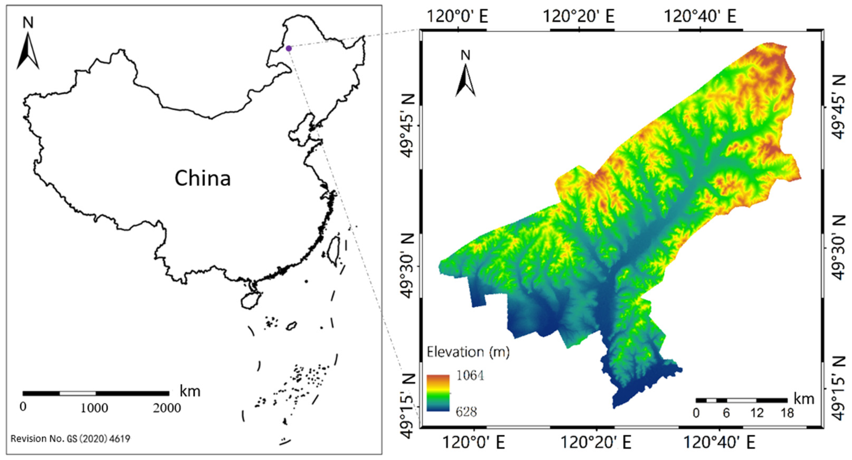
Tenihe Farm was established in July 1955 and comprises 11 planting divisions, representing an agricultural reclamation enterprise with contemporary management. The farm is geographically situated in the northern section of the Daxing’anling Mountains; the eastern and northern parts of the farm fall within the stony mid-mountain subregion of the northern Daxing’anling, while the western and southern parts belong to the stony low-mountain subregion of the northern Daxing’anling’s western slope [14]. The overall topography is characterized by lower elevations in the west and higher elevations in the east, with a regional distribution of rocks, among which granite occupies a significant area. Together with other types of igneous rocks, these rocks form a terrain that combines plains with mountainous features, thus exhibiting typical riparian geomorphological characteristics [32]. The mountains, shaped by long-term weathering and erosion, have gentle slopes. The total area of the farm is approximately 1900 km², with approximately 670,000 mu of arable land available for cultivation. It is located between 119°45′–120°60′E and 49°10′–49°55′N, with elevations ranging from 628 to 1064 m. The cropping system used for agricultural production is based on a single harvest per year, with land preparation and sowing typically carried out in May and crop harvesting generally completed by October. The water requirements for the crops during the growing season are primarily met with natural precipitation. Owing to antiquated irrigation practices, soil moisture retention has not been adequately maintained. The perennial evaporation of surface water, coupled with the residual crystallization of pesticides and fertilizers, leads to salinization in the arable soil of the farm.

The geographical location and basic information of Tenihe Farm are illustrated in Figure 1 below.

2.2. Data Preparation

The data utilized in this article were constructed through the Google Earth Engine (GEE) platform, accessed on 10 January 2024 at https://developers.google.com/earth-engine/datasets/catalog/landsat, to establish a Landsat dataset. This involved the acquisition of Landsat satellite imagery data spanning the crop growing seasons from 2013 to 2022, specifically from April to October each year. The images underwent radiometric calibration, atmospheric correction, mosaicking, and cropping processes to yield mean composite data for the study area. Subsequent calculations and processing were conducted for the IRSEI. The period from April to October coincides with the crop growth and harvesting season, and it is also the peak growth phase for surrounding vegetation, suggesting that this period is an opportune time for vegetation detection. Employing the IRSEI method facilitates a more reliable assessment of ecological conditions [33].

The acquired imagery data necessitate a series of preprocessing steps prior to the computation of indices to enhance the accuracy of subsequent spectral band calculations. The rationale behind preprocessing is that detectors and other instruments are influenced by factors such as atmospheric radiation, the satellite’s orientation during flight, the solar zenith angle, and the conditions of the Earth’s surface coverage. Moreover, the multitude of radiometric information obtained through remote sensing methods undergoes physical alterations such as absorption or scattering upon interaction with the atmosphere, leading to the attenuation of the radiative energy and, consequently, introducing errors into the spectral information captured. Preprocessing enables the correction of distortions in remote sensing imagery, as well as the reduction or elimination of noise interference, thereby ensuring more accurate geometric features of the imagery and information content that is more representative of the actual conditions. The remote sensing image preprocessing workflow conducted in this next step primarily encompassed radiometric calibration, atmospheric correction, image mosaicking, image cropping, and the combination of image bands. Notably, the atmospheric correction carried out in this study was performed within the GEE framework using the sensor-invariant atmospheric correction (SIAC) method [34].

3. Methods

The ecological quality assessment method proposed in this paper is based on remote sensing techniques. In agricultural planting areas, ecological quality is generally represented as a comprehensive quality evaluation, via a coupled component indicator approach. These component indicators include vegetation coverage, ecological moisture, aridity, thermal conditions, and the degree of soil salinization within the farm region. After the indicators that affect agricultural planting areas through objective and reliable remote sensing data are quantified, a mathematical transformation is then applied to generate a comprehensive evaluation index. Building upon the RSEI, this paper introduces the improved remote sensing ecological index (IRSEI) method, which was tailored to the study area. In addition to the conventional four indicators, the integrated salinity index (ISI) was innovatively integrated, thereby enabling a more accurate reflection of the true ecological quality of the research area.

3.1. Overview

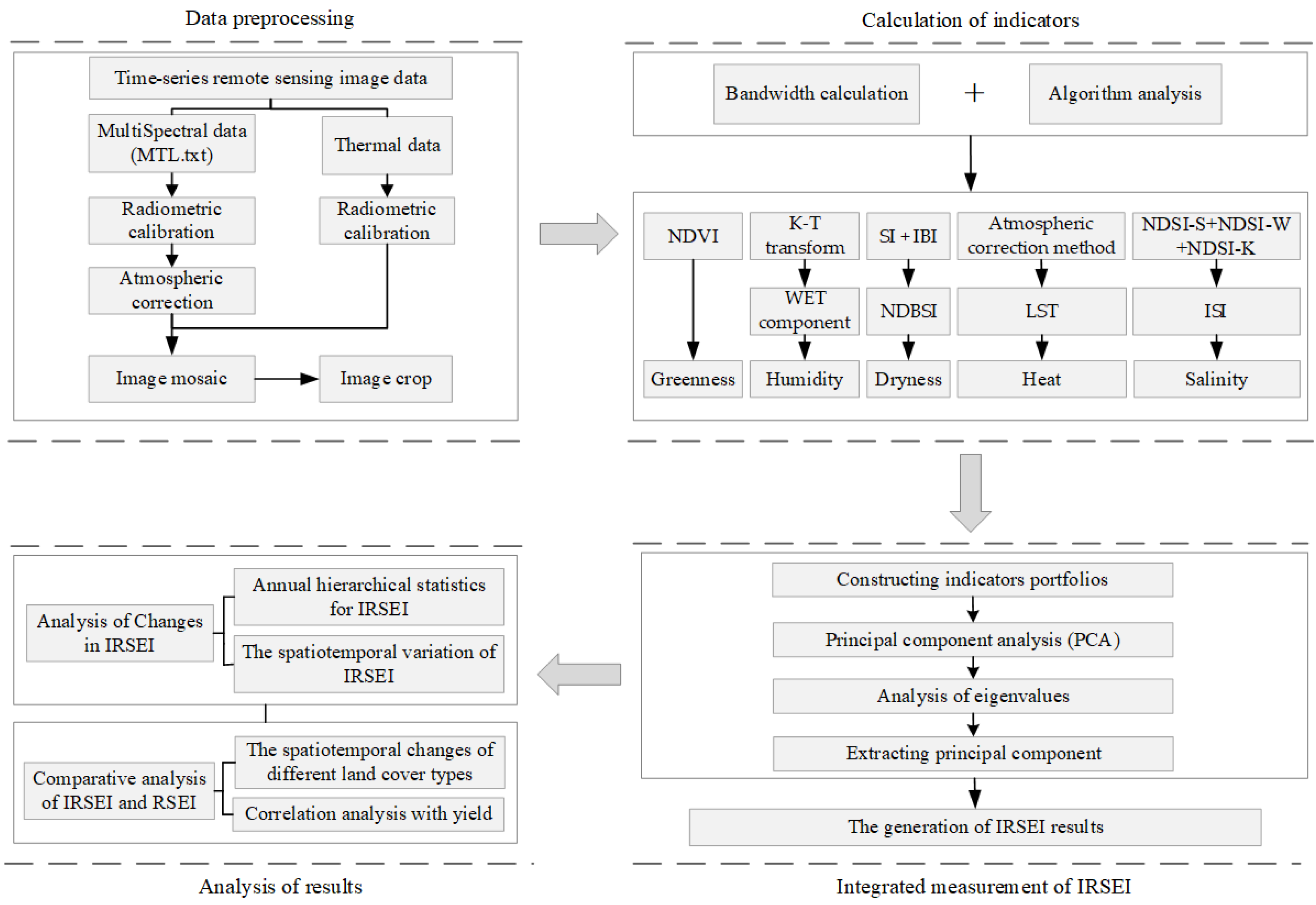
The experimental procedure of the present study is illustrated in Figure 2. The specific steps were as follows: First, preprocessing operations on remote sensing imagery were conducted, which primarily involved the radiometric calibration and atmospheric correction of the raw remote sensing images, followed by the mosaicking and cropping of the corrected images to ensure that the cropped images were well suited to the study area’s boundaries. Second, the five component indices of the IRSEI were computed, and these indices were calculated according to several previous studies [35,36,37,38,39]. Through the dissection of algorithms, the most appropriate expressions were selected, and several algorithmic models were transformed into parameter settings for the computation of remote sensing image bands, resulting in the acquisition of specific values and distribution characteristics of the component indices. Thirdly, the five component indices—greenness, humidity, dryness, heat, and salinity—were standardized and fused, followed by principal component analysis to obtain statistical information for each component. Subsequently, the first principal component post-transformation was utilized as the representative component encapsulating the primary information of the indices; ultimately, mathematical transformations were applied to obtain quantified results of the IRSEI for the farm within the study area. Fourth, an analysis of the results was conducted, which was divided into two parts. The first part involved categorizing and statistically assessing the IRSEI outcomes according to annual quality grades. The second part entailed a comparative analysis of the IRSEI results against the original RSEI outcomes across different land use types, as well as an analysis of the correlation with crop yields. This made it possible to evaluate the advantages of the IRSEI method.

3.2. Calculation of Component Indicators

Prior to the comprehensive computation of the IRSEI, it is imperative to explore and calculate the component indices within the IRSEI framework. As critical constituents in the assessment of the ecological environmental quality of farm research areas, these component indices need to be precisely controlled to provide an accurate foundation for the subsequent coupling of component indices. The theoretical underpinnings and specific calculation methods for the five component indices—greenness, humidity, dryness, heat, and salinity—are elaborated upon in detail below.

3.2.1. Calculation of the Greenness Index

In the context of the IRSEI framework, the greenness index is an important indicator of the quality of the ecological environment. This paper utilizes the normalized difference vegetation index (NDVI) to characterize the greenness index [40]. Vegetation, as a vital component of ecosystems, plays an indispensable role in the Earth’s carbon cycle and climate dynamics. The NDVI is a commonly used remote sensing index that can also be employed for assessing and monitoring the condition and growth of vegetation. Specifically, the greenness and growth status of vegetation are reflected by calculating the difference between the infrared and visible light bands in remote sensing images. The formula for calculating the NDVI is as follows:

$$NDVI=\frac{{\rho }_{NIR}-{\rho }_{Red}}{{\rho }_{NIR}+{\rho }_{Red}}$$

(1)

where ${\rho }_{NIR}$ represents the reflectance in the near-infrared band, and ${\rho }_{Red}$ represents the reflectance in the visible light red band. The $NDVI$ values ranged from −1 to 1, with higher values indicating more vegetation cover and lower values indicating less vegetation cover.

3.2.2. Calculation of the Humidity Index

The humidity index primarily characterizes the moisture content of vegetation and soil within image coverage. This index is extensively employed across various domains, such as ecological monitoring and evaluation [41,42,43]. The humidity index can be represented using the WET component of the tasseled cap transform (TCT), also known as the K-T transform. The WET component is essentially a feature component generated through the K-T transform [44]. The K-T transform can be viewed as a specialized form of principal component analysis (PCA). However, a notable distinction is that, unlike conventional PCA, the K-T transform utilizes a fixed transformation matrix. The K-T transform introduces a constant matrix into the digitized original remote sensing image and translates it into a new feature space with which humidity can be aptly transformed to obtain results. The transformed components can enhance image information and effectively represent spatial moisture content. The transformation formula is as follows:

$$B=\lambda A$$

(2)

where $B$ represents the image after the K-T transformation, $\lambda$ denotes the matrix coefficients of the transformation, and $A$ signifies the original image. To perform a K-T transformation on remote sensing images, it is necessary to obtain information about the transformation matrix coefficients. The transformation matrix coefficients vary with the different settings of the satellite sensors; thus, the coefficient settings of the WET calculation formula are not identical. Expert experience can guide the humidity calculation formula, corresponding to different Landsat satellite sensors through different parameter settings [41,42]. The specific settings of the transformation matrix coefficients for the humidity indices are shown in

Table 1. K-T transformation matrix coefficients of Landsat series satellites.

	Band	Blue	Green	Red	NIR	SWIR1	SWIR2
Sensor
Landsat TM		0.0315	0.2021	0.3102	0.1594	0.6806	0.6109
Landsat ETM+		0.1509	0.1973	0.3279	0.3406	0.7112	0.4572
Landsat OLI		0.1511	0.1973	0.3283	0.3407	0.7117	0.4559

below.

Through the configuration of different K-T transformation matrix coefficients, various WET index calculation formulas for different sensors can be derived, as shown below:

The WET index calculation formula for Landsat 5 TM is as follows:

$$\begin{array}{ll}WE{T}_{(TM)}=& 0.0315{\rho }_{Blue}+0.2021{\rho }_{Green}+0.3102{\rho }_{Red}+0.1594{\rho }_{NIR}-\\ & 0.6806{\rho }_{SWIR1}-0.6109{\rho }_{SWIR2}\end{array}$$

(3)

The WET index calculation formula for Landsat 7 ETM+ is as follows:

$$\begin{array}{ll}WE{T}_{(ETM)}=& 0.1509{\rho }_{Blue}+0.1973{\rho }_{Green}+0.3279{\rho }_{Red}+0.3406{\rho }_{NIR}-\\ & 0.7112{\rho }_{SWIR1}-0.4572{\rho }_{SWIR2}\end{array}$$

(4)

The WET index calculation formula for Landsat 8 OLI is as follows:

$$\begin{array}{ll}WE{T}_{(OLI)}=& 0.1511{\rho }_{Blue}+0.1973{\rho }_{Green}+0.3283{\rho }_{Red}+0.3407{\rho }_{NIR}-\\ & 0.7117{\rho }_{SWIR1}-0.4559{\rho }_{SWIR2}\end{array}$$

(5)

In the aforementioned three equations, ${\rho }_{Blue}$ represents the reflectance in the blue band, ${\rho }_{Green}$ denotes the reflectance in the green band, ${\rho }_{Red}$ signifies the reflectance in the red band, ${\rho }_{NIR}$ corresponds to the reflectance in the near-infrared band, ${\rho }_{SWIR1}$ is indicative of the reflectance in the shortwave infrared-1 band, and ${\rho }_{SWIR2}$ stands for the reflectance in the shortwave infrared-2 band. A higher WET value suggests increased humidity.

3.2.3. Calculation of the Dryness Index

Due to the presence of human settlements and construction areas in the study area, as well as the existence of bare soil, the aridity index in this chapter is characterized using a composite approach combining the Building Index and the Bare Soil Index. These two indices can, to some extent, reflect the condition of soil health, soil aridification phenomena, and consequently, to a certain degree, the changes and quality of the local ecological environment. The aridity index, known as the normalized difference build and soil index (NDBSI) [45], is calculated by adding the soil erosion index (SI) [46] and the index-based build-up index (IBI) [47] and then averaging the result. The specific formulas are as follows:

$$NDBSI=(SI+IBI)/2$$

(6)

$$SI=[({\rho }_{SWIR1}+{\rho }_{Red})-({\rho }_{NIR}+{\rho }_{Blue})]/[({\rho }_{SWIR1}+{\rho }_{Red})+({\rho }_{NIR}+{\rho }_{Blue})]$$

(7)

$$\begin{array}{ll}IBI=& \{2{\rho }_{SWIR1}/({\rho }_{SWIR1}+{\rho }_{NIR})-[{\rho }_{NIR}/({\rho }_{NIR}+{\rho }_{Red})+{\rho }_{Green}/({\rho }_{Green}+{\rho }_{SWIR1})]\}/\\ & \{2{\rho }_{SWIR1}/({\rho }_{SWIR1}+{\rho }_{NIR})+[{\rho }_{NIR}/({\rho }_{NIR}+{\rho }_{Red})+{\rho }_{Green}/({\rho }_{Green}+{\rho }_{SWIR1})]\}\end{array}$$

(8)

In this context, ${\rho }_{SWIR1}$ represents the reflectance in the shortwave infrared 1 (SWIR1) band, ${\rho }_{Red}$ represents the reflectance in the visible red band, ${\rho }_{NIR}$ represents the reflectance in the near-infrared band, ${\rho }_{Blue}$ represents the reflectance in the visible blue band, and ${\rho }_{Green}$ represents the reflectance in the visible green band. The values of these parameters typically range from −1 to 1. These indicators characterize two types of content, namely, content that enhances dryness and content that reduces dryness; the enhancing content typically includes buildings and bare soil, while content that reduces dryness includes vegetation and water bodies, among others.

3.2.4. Calculation of the Heat Index

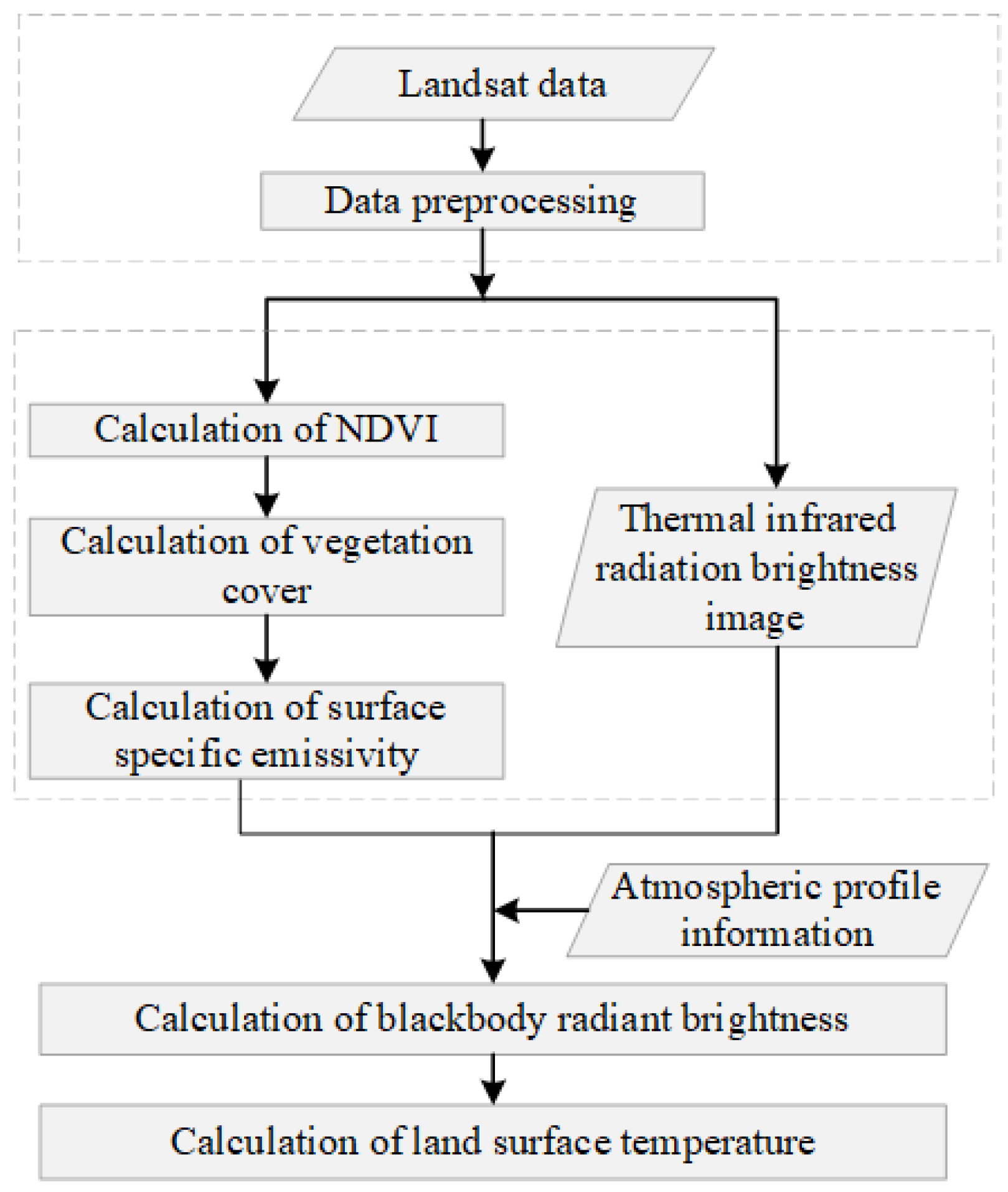
This study investigated the use of land surface temperature (LST) as a representation of heat [48]. The thermal infrared bands of the Landsat satellite series are sensitive to the thermal radiation of surface coverings, allowing them to be extensively utilized in monitoring LST variations [49]. Regarding LST computations, there are two conventional methodologies: the single-channel algorithm and the multichannel algorithm. The single-channel algorithm encompasses methods such as atmospheric correction (also referred to as the radiative transfer equation), the universal single-channel method, and the single-window algorithm. The multichannel algorithm primarily includes the split-window algorithm and the temperature emissivity separation algorithm. In this chapter, the atmospheric correction method is adopted for LST inversion. The principle of calculating surface temperature using the atmospheric correction method involves initially aggregating the total thermal radiation detected via the satellite sensor. Subsequently, various techniques have been employed to simulate and quantify the influence of the atmosphere on surface thermal radiation. The total thermal radiation is subsequently reduced by the radiation amount consumed by atmospheric effects, yielding the actual thermal radiation at the surface. This genuine surface thermal radiation undergoes mathematical transformation to derive the inverted surface temperature. The process of calculating surface temperature using the atmospheric correction method is illustrated in Figure 3.

Figure 3 shows that the computation of LST necessitates several intermediary steps, involving the acquisition of remote sensing imagery and some preprocessing routines, as well as the calculation of certain indices and parameter retrieval. The specific intermediary processes and steps are described in detail below.

(1)

Image preprocessing

This paper divides the preprocessing of remote sensing imagery into two distinct segments. The initial segment pertains to the processing of multispectral data (MTL.txt), with a preprocessing sequence encompassing radiometric calibration, atmospheric correction, image mosaicking, and image cropping. The second segment addresses image preprocessing for thermal infrared data and follows a procedure of radiometric calibration, image mosaicking, and image cropping. These divergent image preprocessing methodologies are tailored to accommodate the disparities in computational approaches for different component indices. For instance, prior to the computation of indices such as greenness, wetness, dryness, and salinity, the first preprocessing method is needed. Conversely, the computation of the thermal index necessitates radiometric calibration information from the thermal infrared band, thereby integrating both preprocessing techniques.

(2)

NDVI calculation

The calculation of the NDVI is synonymous with the computation of the greenness index, as shown in Formula (1).

(3)

Vegetation cover calculation

Vegetation cover is primarily calculated by comparing the vertical projection surface of vegetation to the overall study area, including branches, stems, and leaves in the projection. Numerous studies have focused on estimating vegetation cover using remote sensing methods, among which vegetation indices are a frequently applied approach. A commonly used vegetation index is expressed as $NDVI$. The vegetation cover calculation outlined in this chapter was calculated mainly through $NDVI$. In the imagery, areas with and without vegetation cover, as well as monotypic vegetated areas, are visible. Vegetation cover was characterized by calculating the ratio of the difference between $NDVI$ and the nonvegetated area to the difference between completely vegetated and nonvegetated areas. The formula can be expressed as follows:

$$FV=(NDVI-NDV{I}_S)/(NDV{I}_V-NDV{I}_S)$$

(9)

Here, $FV$ represents the magnitude of vegetation coverage, $NDV{I}_S$ denotes the $NDVI$ value for areas devoid of vegetation coverage, and $NDV{I}_V$ signifies the $NDVI$ value for completely vegetated areas. In the experiments of this chapter, based on empirical evidence, $NDV{I}_S$ and $NDV{I}_V$ were set to 0.05 and 0.7, respectively. This implies that, when the value of $NDVI$ within a pixel exceeded 0.7, the value of $FV$ was set to 1; when the value of $NDVI$ within a pixel was less than 0.05, the value of $FV$ was set to 0 [50].

By integrating the formula for vegetation coverage with the set parameters for $NDV{I}_V$ and $NDV{I}_S$, the formula can be transformed into a band calculation method. The band calculation formula is as follows:

$$\begin{array}{ll}FV=& (b1 gt 0.7)\times 1+(b1 lt 0.05)\times 0+(b1 ge 0.05 and b1 le 0.7)\times ((b1-0.05)/\\ & (0.7-0.05))\end{array}$$

(10)

Herein, $b1$ is the result of $NDVI$.

(4)

Calculation of surface emissivity (SE)

Based on prior research, remote sensing images are categorized into three types: water bodies, urban areas, and natural surfaces [51]. In this chapter, the following methodology is adopted to compute the surface emissivity for the study area: the emissivity value for water body pixels was set to 0.995, while the emissivity estimates for natural surface pixels and urban pixels were represented by ${\epsilon }_{surface}$ and ${\epsilon }_{building}$, respectively [50,51]. The specific formulas are as follows:

$${\epsilon }_{surface}=0.9625+0.0614FV-0.0461F{V}^2$$

(11)

$${\epsilon }_{building}=0.9589+0.086FV-0.0671F{V}^2$$

(12)

Incorporating these parameters allows the equation to be transformed into a band calculation method. The formula for band calculation is as follows:

$$\begin{array}{l}{S}_E=(b1 le 0)\times 0.995+(b1 gt 0 and b1 lt 0.7)\times (0.9589+0.086\times b2-\\ 0.0671\times b2\times b2)+(b1 ge 0.7)\times (0.9625+0.0614\times b2-0.0461\times b2\times b2)\end{array}$$

(13)

where $S_E$ denotes the surface reflectance ratio, $b1$ represents the value of $NDVI$, and $b2$ signifies the vegetation cover fraction $FV$.

(5)

Calculation of blackbody radiance values under identical temperature conditions

The computation of radiance values involves three types of radiative signals received via the detector from the Landsat satellite. The first signal pertains to the atmospheric transmittance in the thermal infrared band, which represents the portion of ground-level radiance that, after being filtered through the atmosphere, is captured via the satellite sensor ($t$). The second signal is the upward atmospheric radiance ($L_u$). The third signal is the energy reflected back after being radiated downward by the atmosphere and received via the detector ($L_d$). These three sets of data can be accessed from a website published by NASA (http://atmcorr.gsfc.nasa.gov/, accessed on 1 January 2024). Upon acquiring the values of $t$, $L_u$, and $L_d$, the formula for calculating the brightness value (L) of thermal infrared radiation received via the satellite can be expressed as follows:

$$L=[S_E{B}_T+(1-S_E)L_d]t+L_u$$

(14)

where $T$ represents the true surface temperature, $S_E$ denotes the surface emissivity, $t$ signifies the atmospheric transmittance under thermal infrared conditions, and $B_T$ represents the blackbody brightness value of thermal radiation.

From the aforementioned equation, the brightness $B_T$ of the blackbody radiation in the thermal infrared band at temperature $T$ can be derived, and the formula is presented as follows:

$$B_T=[L-L_u-t(1-S_E)L_d]/t{S}_E$$

(15)

Through the intervention of the inverse function of Planck’s law, the surface temperature can be obtained. The actual surface temperature obtained at this point is expressed in Kelvin (K), not the Celsius (°C) unit commonly used in general contexts. Consequently, a conversion of temperature units is needed. Converting Kelvin to Celsius merely necessitates subtracting 273.15 from the original temperature. Hence, the expression for LST is as follows:

$$LST=K_2/\ln K_1/(B_T+1)-273.15$$

(16)

In this context, $K_1$ and $K_2$ represent predefined constants prior to the satellite launch. The settings for $K_1$ and $K_2$ for different sensor types of Landsat satellites are presented in

Table 2. Settings of K₁ and K₂ for different sensor types.

Sensor Types	K1	K2
Landsat 5 TM (band 6)	607.76	1260.56
Landsat 7 ETM+ (band 6)	666.09	1282.71
Landsat 8 TIRS (band 10)	774.89	1321.08
Landsat 8 TIRS (band 11)	480.89	1201.14

.

Due to the susceptibility of the 11th band of Landsat 8 TIRS to interference from stray light and other noise, calibration can introduce significant biases. If introduced into calculations, this approach may compromise the accuracy of subsequent results [52]. Hence, this study utilizes the 10th shortwave band of Landsat 8 TIRS for computation, employing the corresponding K₁ and K₂ values from the table for analysis.

When translated into band calculation format, the formula is as follows:

$$LS{T}_b=K_2/a\log (K_1/b1+1)-273.15$$

(17)

Within this context, b1 represents the blackbody radiance image under identical temperature conditions.

From this, the Celsius temperature band calculation formula for Landsat 5 TM can be derived as follows:

$$LS{T}_5=1260.56/a\log (607.76/b1+1)-273.15$$

(18)

The Celsius temperature band calculation formula for Landsat 7 ETM+ is as follows:

$$LS{T}_7=1282.71/a\log (666.09/b1+1)-273.15$$

(19)

The Celsius temperature band calculation formula for Landsat 8 TIRS is as follows:

$$LS{T}_8=1321.08/a\log (774.89/b1+1)-273.15$$

(20)

where b1 are the blackbody radiance brightness images for the same temperature conditions.

3.2.5. Calculation of the Salinity Index

Soil salinity serves as an effective evaluative metric for the degree of soil salinization. Given that the visible and near-infrared spectral bands of remote sensing exhibit certain responses to soil salinity, it is feasible to consider the estimation of soil salinity information via remote sensing techniques. Recently, inversion research on soil salinity indices using remotely sensed spectral information has garnered growing attention. This method holds advantages for large-scale monitoring, offering benefits such as a continuous temporal sequence and the strong timeliness of data. The results of remote sensing inversion estimations can also serve as a reference, providing assistance for subsequent soil environmental remediation and land reclamation efforts [53]. This paper employs an integrated salinity index (ISI) that integrates three different remote sensing salinity indices to quantify the soil salinity index of the study area. The first method of integration is the SI-S method [54], which utilizes the red, green, blue, and near-infrared spectral bands for the estimation of the soil salinity index. The calculation formula is as follows:

$$SI-S=\sqrt{\frac{({\rho }_{NIR}\times {\rho }_{Red})-({\rho }_{Green}\times {\rho }_{Blue})}{({\rho }_{NIR}\times {\rho }_{Red})+({\rho }_{Green}\times {\rho }_{Blue})}}$$

(21)

In this context, ${\rho }_{NIR}$ denotes the reflectance of the near-infrared band, ${\rho }_{Red}$ represents the reflectance of the red band, ${\rho }_{Green}$ signifies the reflectance of the green band, and ${\rho }_{Blue}$ corresponds to the reflectance of the blue band.

The second fusion method is the SI-W method [55], which utilizes the red and green bands to estimate the soil salinity index. The calculation formula is presented below:

$$SI-W=({\rho }_{Green}+{\rho }_{Red})/2$$

(22)

where ${\rho }_{Green}$ represents the reflectance of the green band, and ${\rho }_{Red}$ denotes the reflectance of the red band.

The third fusion method is the SI-K method [56], which employs the red band and the near-infrared band to estimate the soil salinity index. The calculation formula is as follows:

$$SI-K=({\rho }_{Red}-{\rho }_{NIR})/({\rho }_{Red}+{\rho }_{NIR})$$

(23)

where ${\rho }_{Red}$ represents the reflectance of the red band, and ${\rho }_{NIR}$ denotes the reflectance of the near-infrared band.

Fusion is conducted by adding the values and then calculating the mean. Prior to fusion, the three indices are normalized to constrain the values within the range of 0 to 1. Given that the SI-S index is negatively correlated with the soil salinity index, a positive correlation transformation is performed in advance. The resultant ISI exhibited a positive correlation with the soil salinity conditions in which higher values indicated a greater degree of salinity, and lower values suggested reduced soil salinity. The calculation formula for the ISI is as follows:

$$\begin{array}{l}ISI=(NDSI-S+NDSI-W+NDSI-K)/3\\ =\left(N{D}_{\sqrt{\frac{({\rho }_{NIR}\times {\rho }_{Red})-({\rho }_{Green}\times {\rho }_{Blue})}{({\rho }_{NIR}\times {\rho }_{Red})+({\rho }_{Green}\times {\rho }_{Blue})}}}+N{D}_{({\rho }_{Green}+{\rho }_{Red})/2}+N{D}_{({\rho }_{Red}-{\rho }_{NIR})/({\rho }_{Red}+{\rho }_{NIR})}\right)/3\end{array}$$

(24)

where $NDSI-S$ represents the normalized value of $SI-S$ after a positive correlation transformation, $NDSI-W$ denotes the normalized value of $SI-W$, and $NDSI-K$ indicates the normalized value of $SI-K$.

3.3. Calculation of IRSEI

The principal component analysis (PCA) method is employed to perform a principal component transformation of five indicators. Prior to executing the principal component transformation, it is imperative to normalize the five component indicators. In the experiment of this chapter, the range normalization method was utilized, standardizing the numerical values of the component indicators to a uniform scale between 0 and 1. The computational formula is as follows:

$$R{I}_{norm}=\frac{X-X_{\min }}{X_{\max }-X_{\min }}$$

(25)

where $R{I}_{norm}$ represents the value of the component indicator after standardization, $X$ represents the numerical value of a single indicator, $X_{\max }$ represents the maximum value within the indicator range, and $X_{\min }$ represents the minimum value within the indicator range.

After the principal component transformation, the first principal component often contributes a substantial proportion of the variance and can purely and objectively represent ecological characteristics. The second, third, fourth, and fifth principal components frequently contain disordered information; indiscriminately incorporating them into calculations may bias the final results. Therefore, the first principal component can represent the general trend of comprehensive ecological characteristics. The transformed first principal component, $PC1$, represents the initial remote sensing ecological index value, denoted as $IRSE{I}_0$, and its formula can be expressed as follows:

$$IRSE{I}_0=F_{PC1}(NDVI,WET,NDBSI,LST,ISI)$$

(26)

For the convenience of statistical analysis, it is necessary to standardize $IRSE{I}_0$, yielding $IRSEI$. Hence, $IRSEI$ can be expressed as follows:

$$IRSEI=\frac{IRSE{I}_0-IRSE{I}_{0\min }}{IRSE{I}_{0\max }-IRSE{I}_{0\min }}$$

(27)

where $IRSEI$ represents the value after standardization, $IRSE{I}_0$ represents the initial value of the remote sensing ecological index, $IRSE{I}_{0\min }$ represents the minimum value among the initial values, and $IRSE{I}_{0\max }$ represents the maximum value among the initial values. The interval of $IRSEI$ is between 0 and 1; a high value indicates better ecological quality and a low value indicates poorer ecological quality.

4. Results

4.1. Results of the Component Indicators

To facilitate the presentation of the results, the dimensions were standardized, and the results of the five component indices of the Tenihe Farm IRSEI are displayed using normalized outcomes. The results of component indices spanning from 2013 to 2022 are presented as follows.

4.1.1. Results of the Greenness Index

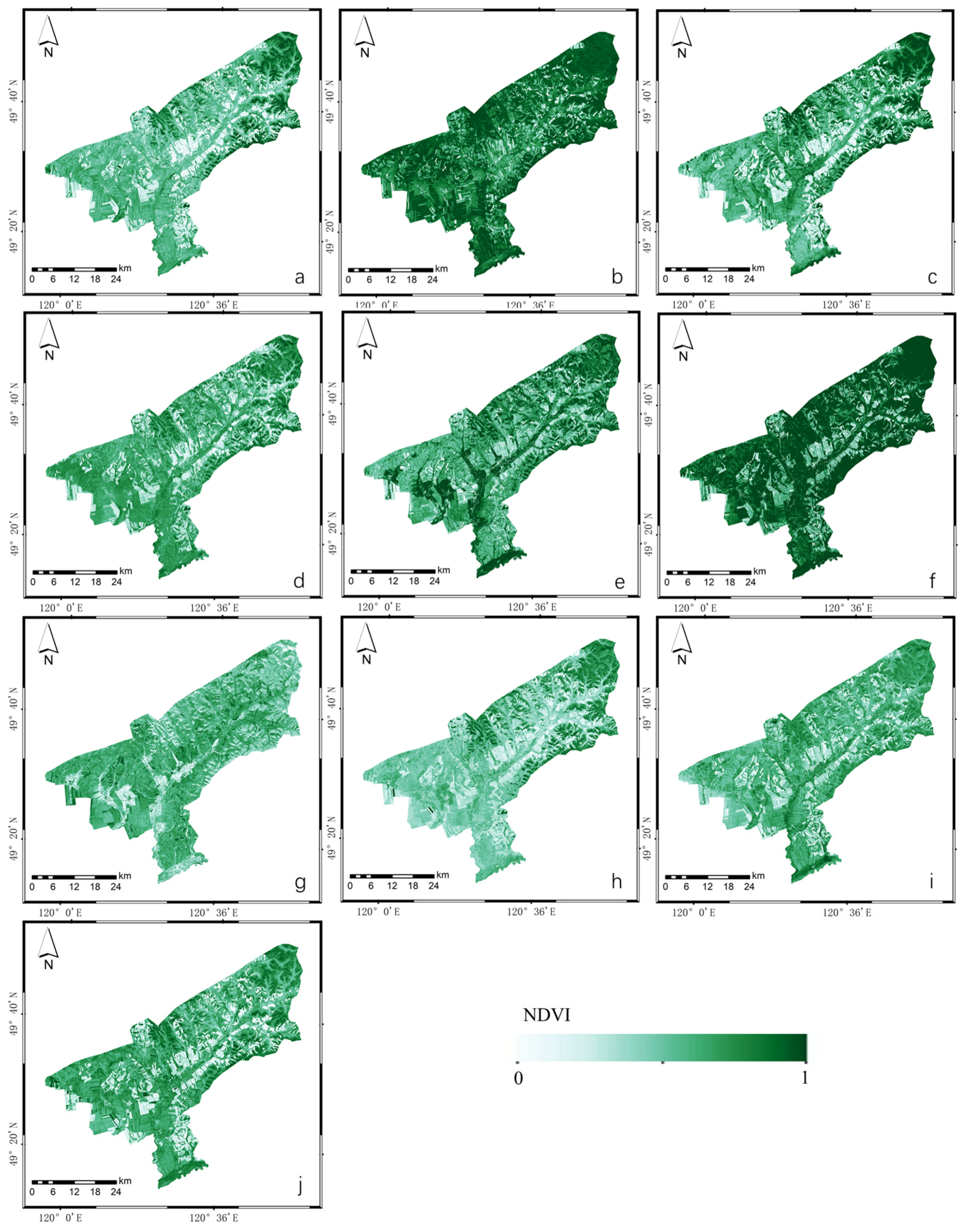
As shown in Figure 4, the remote sensing ecological NDVI data for Tenihe Farm have been favorable over the past decade. Although there have been instances of diminished performance in certain years, the greenness index has remained relatively high for the majority of the period under consideration. This indicates that the vegetation cover in the study area has maintained a consistently positive state over an extended duration.

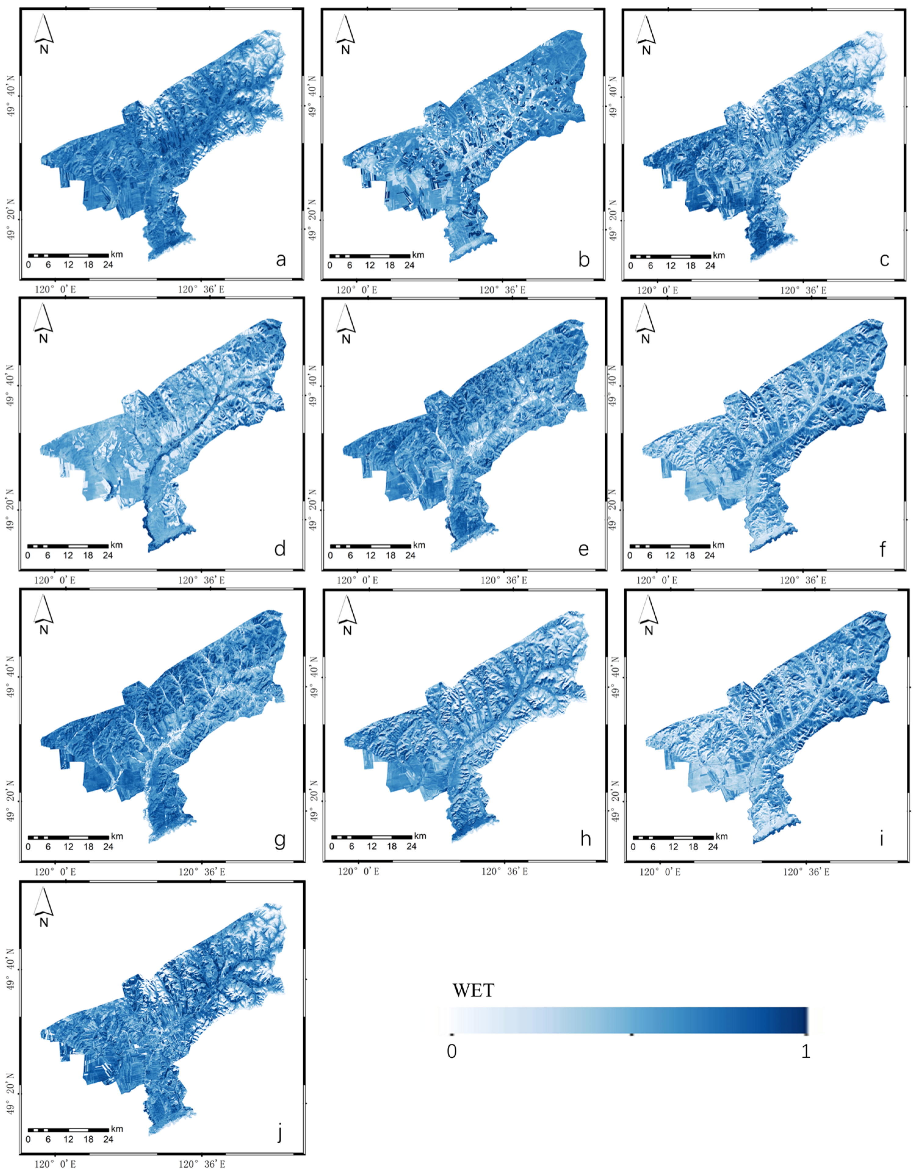
4.1.2. Results of the Humidity Index

Figure 5 reveals that the ecological WET index for Tenihe Farm exhibited relatively stable performance over the course of a decade. The ecological moisture indices for the entire study area demonstrated favorable conditions in recent years, with both soil and surface vegetation maintaining satisfactory levels of moisture.

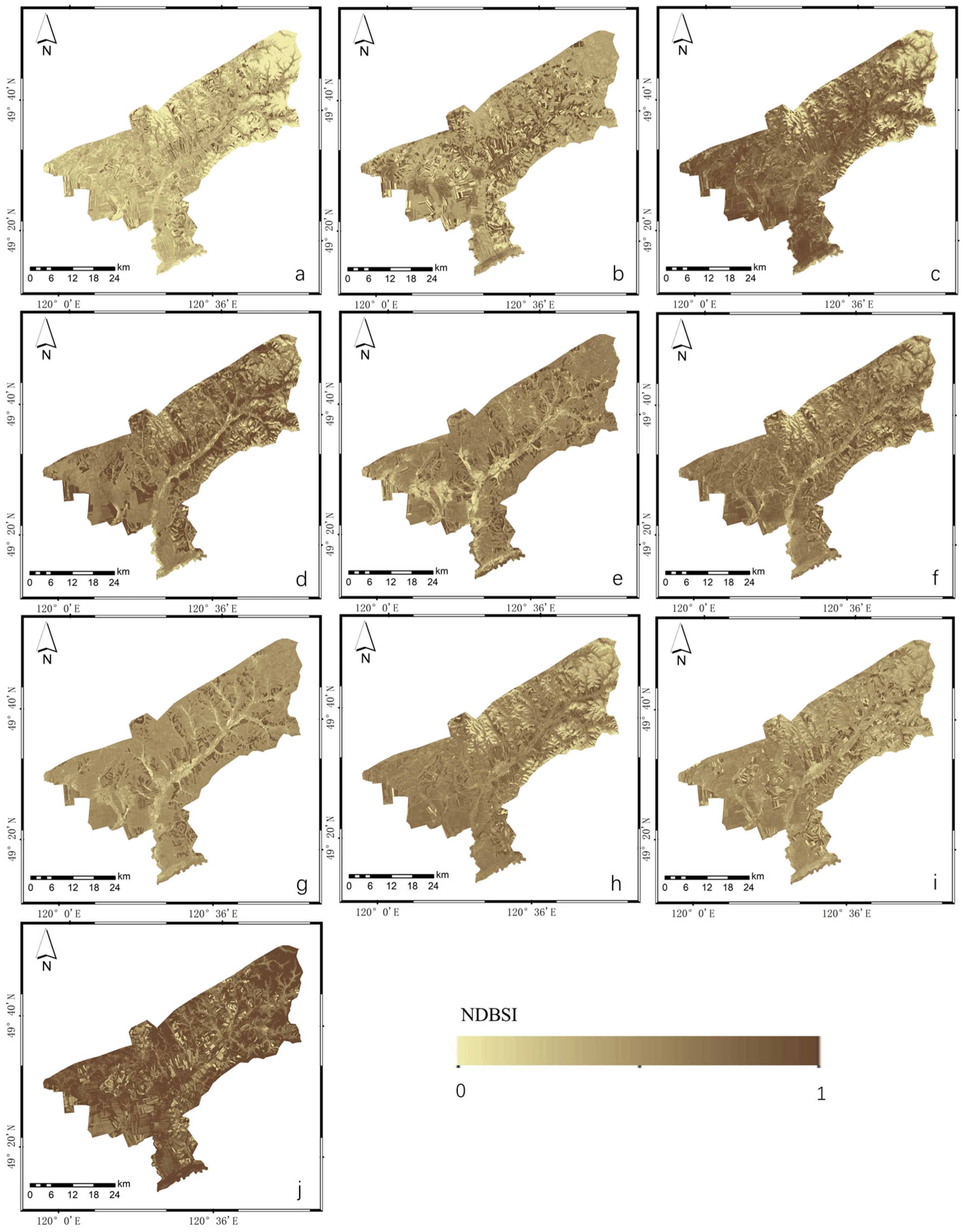
4.1.3. Results of the Dryness Index

Figure 6 indicates that the ecological NDBSI index for Tenihe Farm reflects some variation over the past decade. For instance, in 2013, the NDBSI index exhibited a low value, whereas in 2022, the NDBSI was greater. Theoretically, the NDBSI is considered to exert a negative impact on the ecosystem. However, a comprehensive reflection of the overall ecological index can be ascertained only through an integrated analysis in conjunction with other component indices.

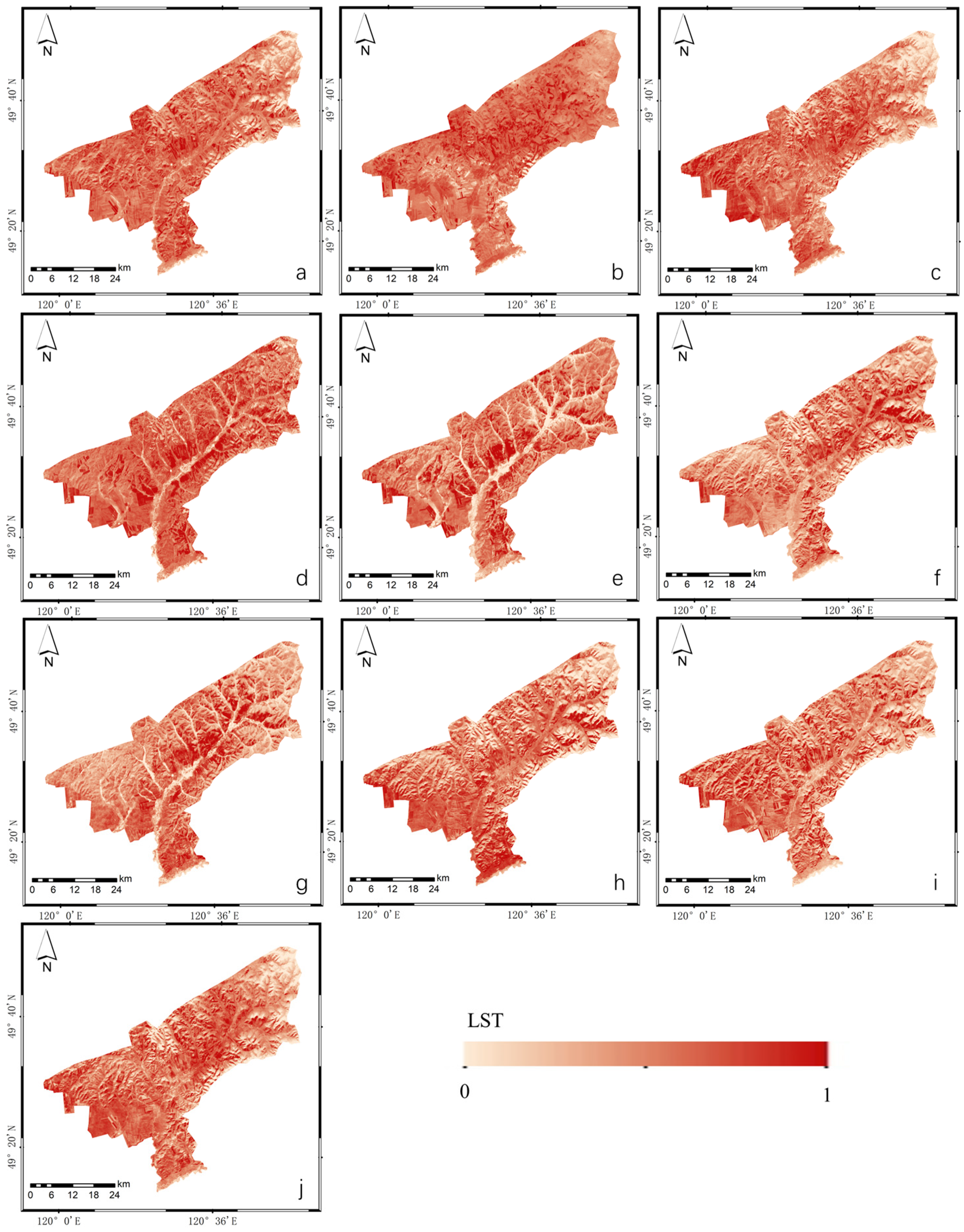
4.1.4. Results of the Heat Index

An analysis of Figure 7 reveals that the ecological LST index for Tenihe Farm has remained relatively stable over the past decade. This suggests that there has been minimal variation in surface temperature during the crop growing season, indicating conditions that are conducive to crop growth.

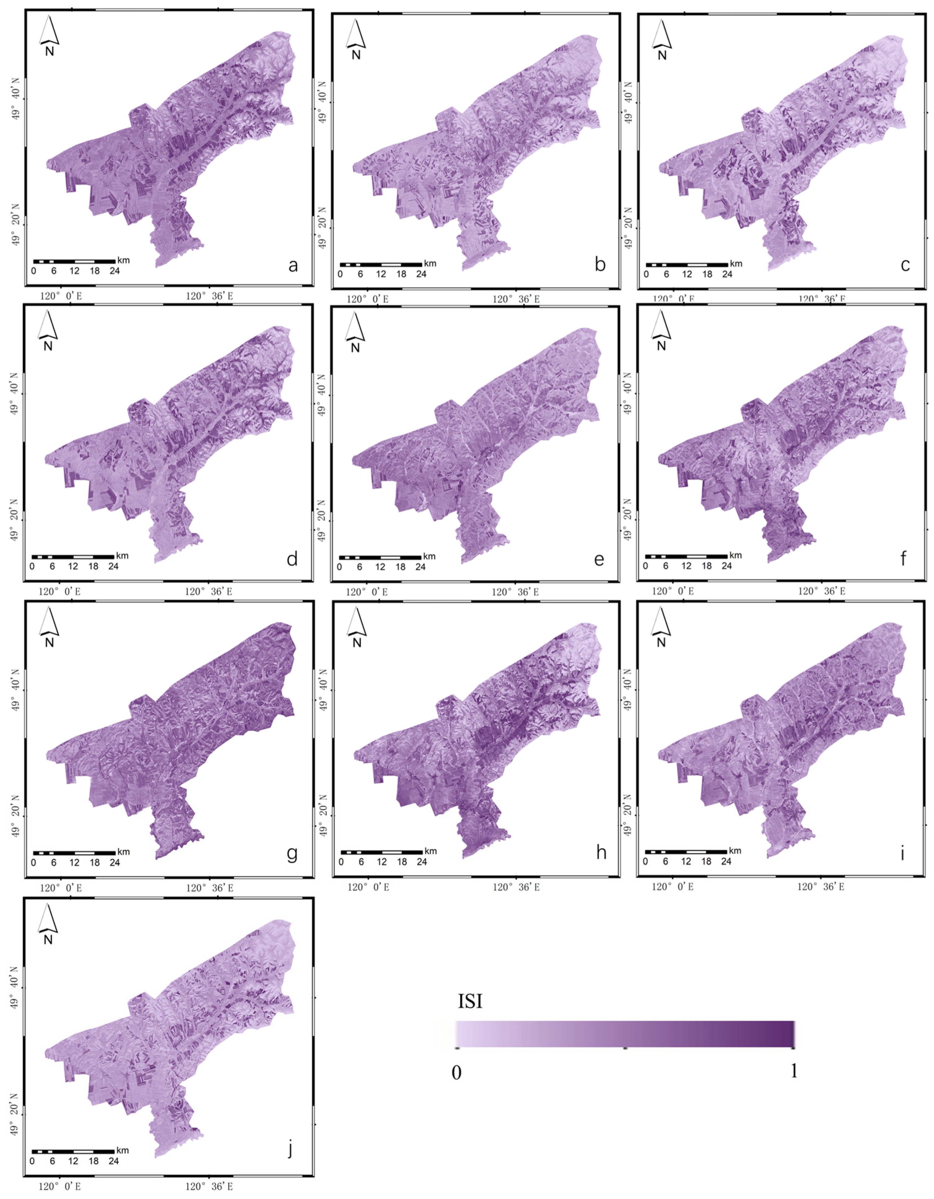
4.1.5. Results of the Salinity Index

As shown in Figure 8, Tenihe Farm has experienced notable salinization over the course of a decade. The areas characterized by agricultural land cover are more impacted by salinization than are the surrounding regions, indicating that prolonged agricultural practices, coupled with the semiarid salinized environmental characteristics of the study area, have perpetuated a state of salinization in the farmlands.

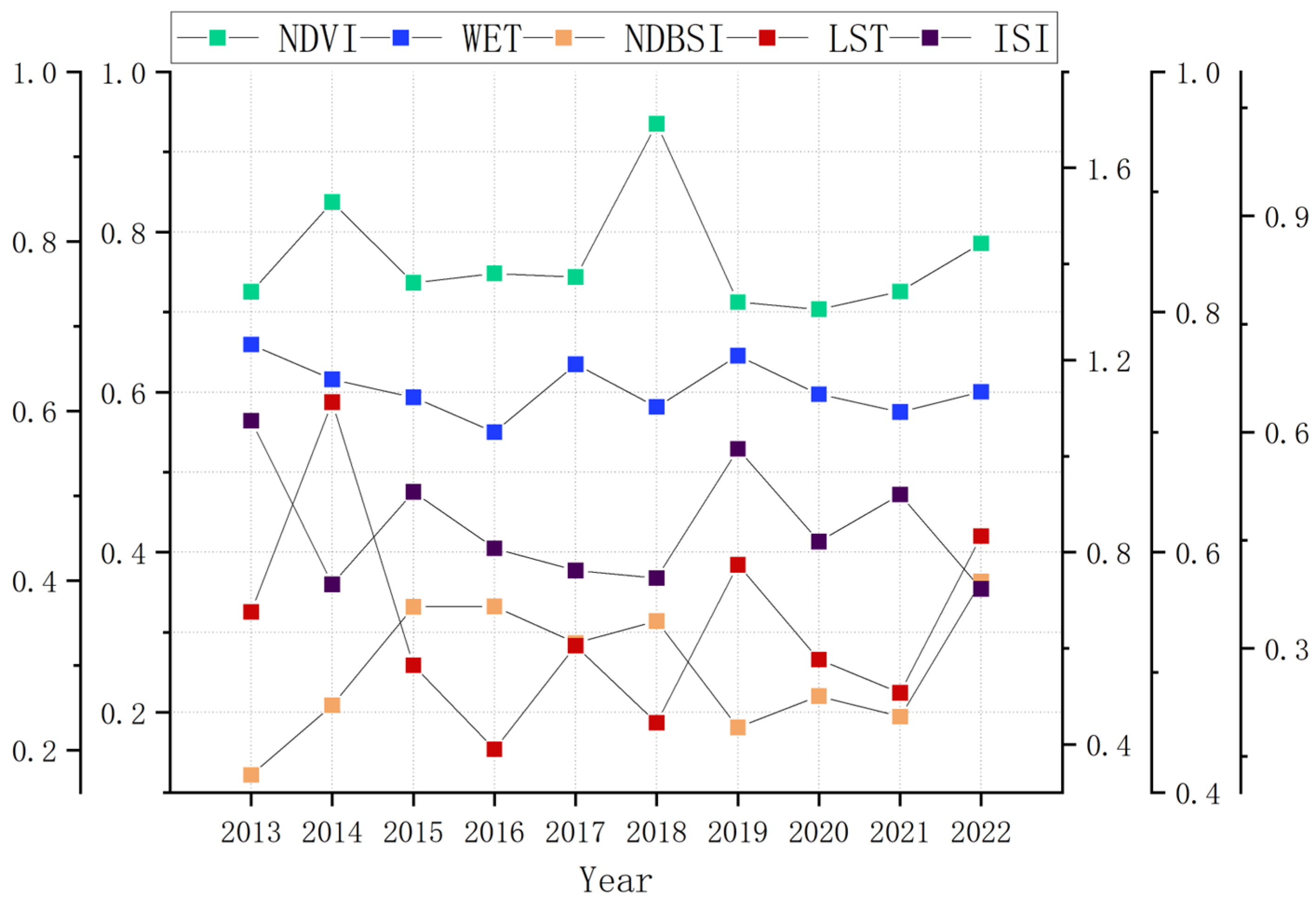
The series of figures presented herein illustrate developmental variations over the course of a decade in the indices of greenness, humidity, dryness, heat, and salinity at Tenihe Farm. These fluctuations indicate that the ecological environment is subject to dynamic transitions. Alterations in the indicators that affect the ecological environment inevitably precipitate a shift in the overall quality of the ecological milieu. The mean values and standard deviations of these five component indices over the ten-year period are depicted in

Table 3. Mean and standard deviation statistics for IRSEI component indicators.

Year	Index	NDVI	WET	NDBSI	LST	ISI
2013	Mean value	0.7253	0.6783	0.3364	0.5504	0.6157
	Standard deviation	0.2248	0.2007	0.0775	0.1941	0.0313
2014	Mean value	0.8373	0.6372	0.4815	0.7249	0.3888
	Standard deviation	0.1836	0.2074	0.2257	0.1127	0.0309
2015	Mean value	0.7365	0.6162	0.6864	0.5058	0.5170
	Standard deviation	0.2405	0.2578	0.2473	0.2230	0.0370
2016	Mean value	0.7483	0.5751	0.6873	0.4360	0.4387
	Standard deviation	0.1737	0.2066	0.2050	0.1843	0.0709
2017	Mean value	0.7438	0.6550	0.6114	0.5222	0.4081
	Standard deviation	0.1904	0.1893	0.1748	0.2231	0.0180
2018	Mean value	0.9350	0.6048	0.6566	0.4581	0.3975
	Standard deviation	0.0999	0.2306	0.1896	0.2281	0.2041
2019	Mean value	0.7124	0.6652	0.4354	0.5896	0.5768
	Standard deviation	0.0435	0.1927	0.0374	0.2227	0.0110
2020	Mean value	0.7036	0.6198	0.5008	0.5106	0.4480
	Standard deviation	0.0542	0.2302	0.0489	0.2550	0.2289
2021	Mean value	0.7257	0.5987	0.4580	0.4829	0.5135
	Standard deviation	0.0529	0.2404	0.0388	0.2359	0.1090
2022	Mean value	0.7856	0.6227	0.7391	0.6134	0.3825
	Standard deviation	0.1450	0.2402	0.0681	0.2243	0.0176

.

Representing the data graphically facilitates a more discernible comprehension of the fluctuations in values. Figure 9 illustrates this representation.

Figure 9 reveals that the values for the five component indices influencing the ecological environment quality at Tenihe Farm have fluctuated and changed over the past decade, a phenomenon attributable to the combined effects of natural factors and human activities. The mean peak values for the greenness, humidity, dryness, heat, and salinity indices were observed in 2014, 2019, 2022, 2014, and 2013, respectively. Conversely, the mean trough values for the greenness, humidity, dryness, heat, and salinity indices were recorded in 2020, 2016, 2013, 2016, and 2022, respectively.

4.2. Results of IRSEI

4.2.1. Validity Analysis of the IRSEI

The component indices were normalized and subsequently transformed through PCA, resulting in a remote sensing image that integrates a novel spectral combination of five principal components. This image constitutes the new representative layer for the IRSEI model, and the eigenvalues for each principal component were ascertained. The eigenvalues and corresponding contribution percentages of the five principal components, PC1, PC2, PC3, PC4, and PC5, post-transformation, offer a more precise delineation of the PCA-derived outcomes. Within the IRSEI framework for the Tenihe Farm experimental zone, the eigenvalues and contribution percentages of the five newly derived principal components after the PCA of the five component indices—NDVI, WET, NDBSI, LST, and PSI—are shown in

Table 4. Results of PCA (eigenvalues and contributions).

Year	Index	PC1	PC2	PC3	PC4	PC5
2013	Eigenvalue	0.1556	0.0206	0.0103	0.0019	0.0008
	Contribution	0.8225	0.1088	0.0546	0.0098	0.0043
2014	Eigenvalue	0.1239	0.0323	0.0152	0.0048	0.0002
	Contribution	0.7021	0.1829	0.0863	0.0275	0.0012
2015	Eigenvalue	0.2298	0.0337	0.0138	0.0029	0.0001
	Contribution	0.8199	0.1203	0.0492	0.0102	0.0004
2016	Eigenvalue	0.1732	0.0257	0.0050	0.0023	0.0007
	Contribution	0.8373	0.1243	0.0242	0.0109	0.0033
2017	Eigenvalue	0.1524	0.0329	0.0113	0.0045	0.0004
	Contribution	0.7562	0.1635	0.0563	0.0222	0.0018
2018	Eigenvalue	0.1830	0.0305	0.0092	0.0033	0.0021
	Contribution	0.8021	0.1337	0.0404	0.0144	0.0094
2019	Eigenvalue	0.0969	0.0221	0.0039	0.0014	0.0004
	Contribution	0.7767	0.1769	0.0316	0.0116	0.0032
2020	Eigenvalue	0.1399	0.0214	0.0149	0.0019	0.0008
	Contribution	0.7822	0.1196	0.0833	0.0105	0.0044
2021	Eigenvalue	0.1001	0.0290	0.0095	0.0022	0.0013
	Contribution	0.7041	0.2041	0.0671	0.0154	0.0093
2022	Eigenvalue	0.1634	0.0266	0.0138	0.0024	0.0007
	Contribution	0.7896	0.1287	0.0666	0.0118	0.0033

.

Table 4 above illustrates that, over the past decade, the contribution of the first principal component (PC1) following the principal component transformation of the IRSEI component indices for the remote sensing imagery covering Tenihe Farm has consistently exceeded 70%. This suggests that PC1 can essentially represent the condition of the farm’s IRSEI. As previously discussed, since PC2, PC3, PC4, and PC5 often contain noisy information, indiscriminately combining principal components is not prudent. The unscientifically based merging of principal components may lead to deviations or even inaccuracies in the results.

To further substantiate the validity of the experimental outcomes, an analysis of data quality was conducted. Typically, indices of greenness and humidity tend to reflect a positive ecological environment condition, whereas indices sensitive to dryness, heat, and salinity are likely to reflect impacted environments, diminishing the quality of the ecological environment assessed. Consequently, when conducting a correlation analysis between these indices and the IRSEI, one would expect to obtain disparate results indicative of both positive and negative correlations. This study employed the Pearson correlation coefficient (PCC) method for the quantitative analysis of the correlation between component indices and the IRSEI. The PCC method is a classical approach to calculating correlation coefficients, and it is primarily used to characterize linear correlations. It operates under the assumption that the two variables in question are normally distributed and possess nonzero standard deviations. The calculation formula condenses values into a range between −1 and 1. The closer the absolute value of the PCC to 1, the greater the degree of correlation between the two variables, indicating greater similarity. The formula for calculating the PCC is as follows:

$$PCC=\frac{{\displaystyle {\sum }_{i=1}^n\left(x_i-\overline{x}\right)\left(y_i-\overline{y}\right)n}}{\sqrt{{\displaystyle {\sum }_{i=1}^n{\left(x_i-\overline{x}\right)}^2}{\displaystyle {\sum }_{i=1}^n{\left(y_i-\overline{y}\right)}^2}}}$$

(28)

In this context, $PCC$ denotes the computed result of the correlation coefficient, $i$ signifies the index associated with the variable, $n$ represents the total number of variables, $x_i$ and $y_i$ respectively correspond to the values of variable $x$ and variable $y$ for index $i$; and $\overline{x}$ and $\overline{y}$ respectively denote the mean values of variable $x$ and variable $y$.

The PCC correlations between the IRSEI outcomes of Tenihe Farm across different years and the component indicators are presented in

Table 5. Correlation analysis between IRSEI results and component indicators over the past decade at Tenihe Farm.

Year	NDVI	WET	NDBSI	LST	PSI	Average Correlation
2013	0.935	0.951	−0.336	−0.874	−0.983	0.816
2014	0.843	0.959	−0.204	−0.985	−0.807	0.771
2015	0.960	0.886	−0.709	−0.837	−0.944	0.867
2016	0.915	0.844	−0.560	−0.974	−0.986	0.856
2017	0.911	0.897	−0.879	−0.966	−0.887	0.908
2018	0.965	0.876	−0.439	−0.934	−0.899	0.823
2019	0.946	0.908	−0.775	−0.942	−0.876	0.889
2020	0.957	0.930	−0.518	−0.896	−0.913	0.843
2021	0.972	0.967	−0.549	−0.906	−0.945	0.868
2022	0.981	0.958	−0.472	−0.927	−0.964	0.860
Mean value	0.939	0.918	−0.544	−0.924	−0.920	p < 0.01

.

Table 5 reveals that the correlation coefficients between different annual component indicators and the IRSEI are both positive and negative, yet they follow a discernible pattern. Specifically, the NDVI and WET are positively correlated with the IRSEI, whereas the NDBSI, LST, and PSI are negatively correlated with the IRSEI. The p-values associated with these correlations were all less than 0.01, indicating statistically significant correlations. Notably, the component indicators for the year 2017 showed the strongest average correlation with the IRSEI, reaching a value of 0.908, while other years also demonstrated high correlation values. The mean values of the five indicators across different years also maintained high levels, with the highest absolute value of correlation in the ten years being for NDVI, at 0.939. This finding suggests that greenness has a substantial impact on ecosystem quality, while other indicators such as heat, humidity, salinity, and dryness are similarly closely linked to the quality of the ecological environment.

4.2.2. Analysis of Spatial and Temporal Variations

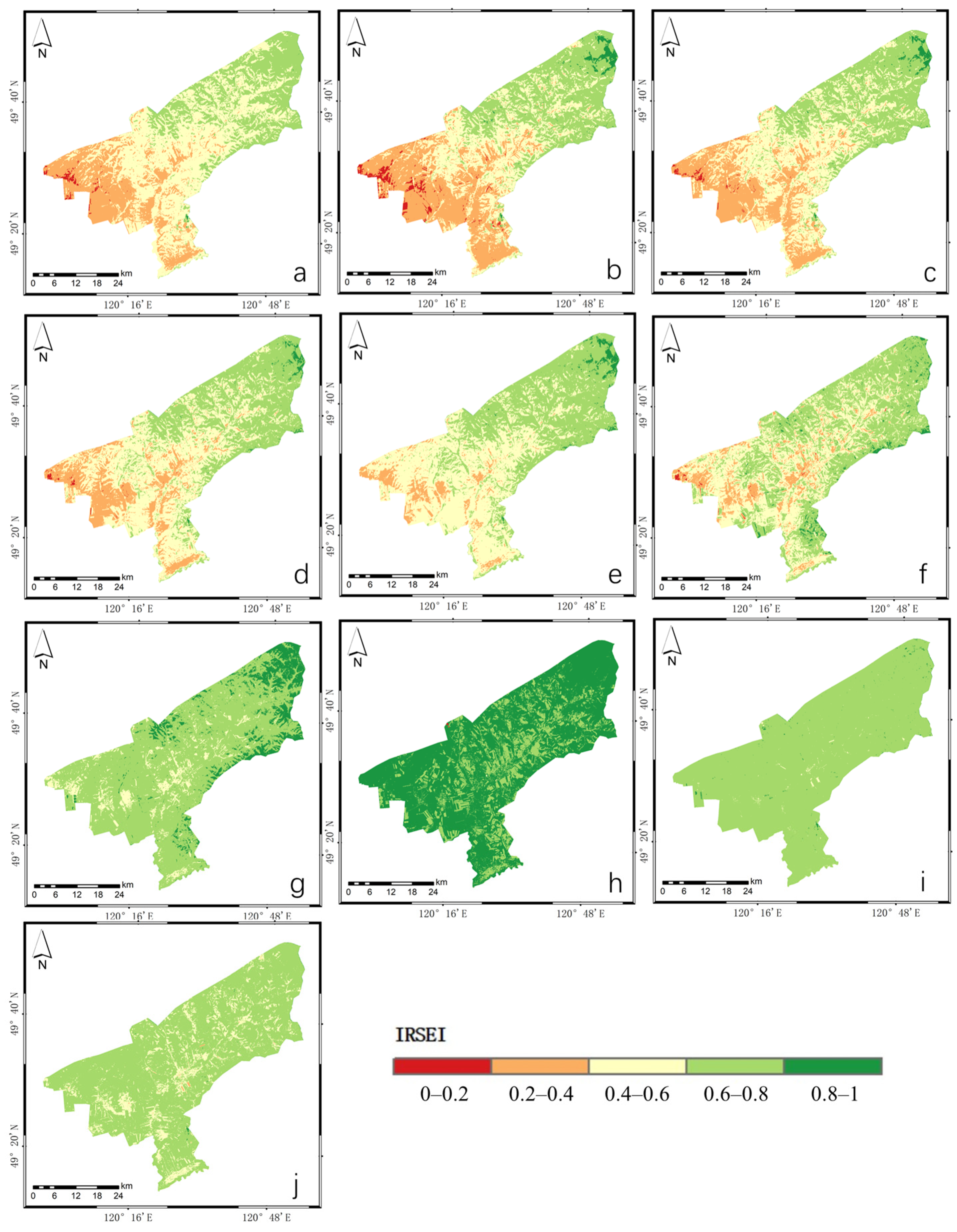
The spatial statistical analysis and cartographic representation of the IRSEI results after principal component transformation reveal clear temporal and spatial variations in the IRSEI scores. The scoring standard employed an interval of 0.2 to divide the values into five categorical levels: excellent (0.8 < RSEI ≤ 1.0), good (0.6 < RSEI ≤ 0.8), moderate (0.4 < RSEI ≤ 0.6), poor (0.2 < RSEI ≤ 0.4), and inferior (0 < RSEI ≤ 0.2). The scoring results are shown in Figure 10.

The graphical representation clearly indicates that the numerical changes and distribution of the IRSEI at Tenihe Farm have varied over the past decade. This variability can be attributed to the differential impacts of various component indices each year, as well as the discrepancies inherent in the representation methods of PCA. The cartographic outcomes suggest that the overall value of the IRSEI is relatively favorable. A detailed quantitative analysis of these results is provided in the subsequent statistical summary.

The mean and standard deviation of the IRSEI for the Tenihe Farm experimental zone over the past ten years are presented in

Table 6. Changes in the mean and standard deviation of the IRSEI at Tenihe Farm over the past decade.

Year	2013	2014	2015	2016	2017	2018	2019	2020	2021	2022
Mean value	0.500	0.500	0.522	0.544	0.584	0.588	0.707	0.826	0.736	0.646
Standard deviation	0.129	0.172	0.153	0.139	0.122	0.133	0.075	0.051	0.039	0.047

. The data reveal remarkable stability in the standard deviation values over the decade, indicating the effectiveness and consistency of the statistical measurements. Specifically, the mean value of the IRSEI reached its peak in 2020, while the lowest point was observed in 2013. The mean IRSEI values from 2013 to 2018 were within the intermediate range (0.4 < IRSEI ≤ 0.6). In contrast, the mean values for 2019, 2021, and 2022 were classified within the good range (0.6 < IRSEI ≤ 0.8), and the mean value for 2020 was categorized within the excellent range (0.8 < IRSEI ≤ 1). This indicates that the ecological quality of Terni Farm exhibited a consistent upward trajectory from 2013 to 2020, followed by a downward trend in the subsequent two years.

The subsequent categorization and area statistics of the IRSEI results across different years are presented in

Table 7. Grading statistics of IRSEI area by year at Tenihe Farm.

Year	Index	Inferior	Poor	Moderate	Good	Excellent
2013	Area/km2	13.82	459.73	986.87	509.53	3.55
	Proportion/%	0.70	23.30	50.01	25.82	0.18
2014	Area/km2	44.23	623.53	652.07	621.16	32.51
	Proportion/%	2.24	31.60	33.04	31.47	1.65
2015	Area/km2	10.16	494.35	794.15	651.32	23.52
	Proportion/%	0.51	25.05	40.24	33.00	1.19
2016	Area/km2	5.15	329.49	916.66	704.86	17.35
	Proportion/%	0.26	16.70	46.45	35.72	0.88
2017	Area/km2	0.00	139.10	959.58	840.48	34.35
	Proportion/%	0.00	7.05	48.62	42.59	1.74
2018	Area/km2	4.63	185.96	800.40	941.05	41.47
	Proportion/%	0.23	9.42	40.56	47.68	2.10
2019	Area/km2	0.00	0.21	172.31	1568.98	232.01
	Proportion/%	0.00	0.01	8.73	79.50	11.76
2020	Area/km2	0.39	0.08	1.23	433.47	1538.33
	Proportion/%	0.02	0.00	0.06	21.96	77.95
2021	Area/km2	0.00	0.05	11.06	1955.49	6.90
	Proportion/%	0.00	0.00	0.56	99.09	0.35
2022	Area/km2	0.00	3.49	286.90	1679.89	3.22
	Proportion/%	0.00	0.18	14.54	85.12	0.16

below.

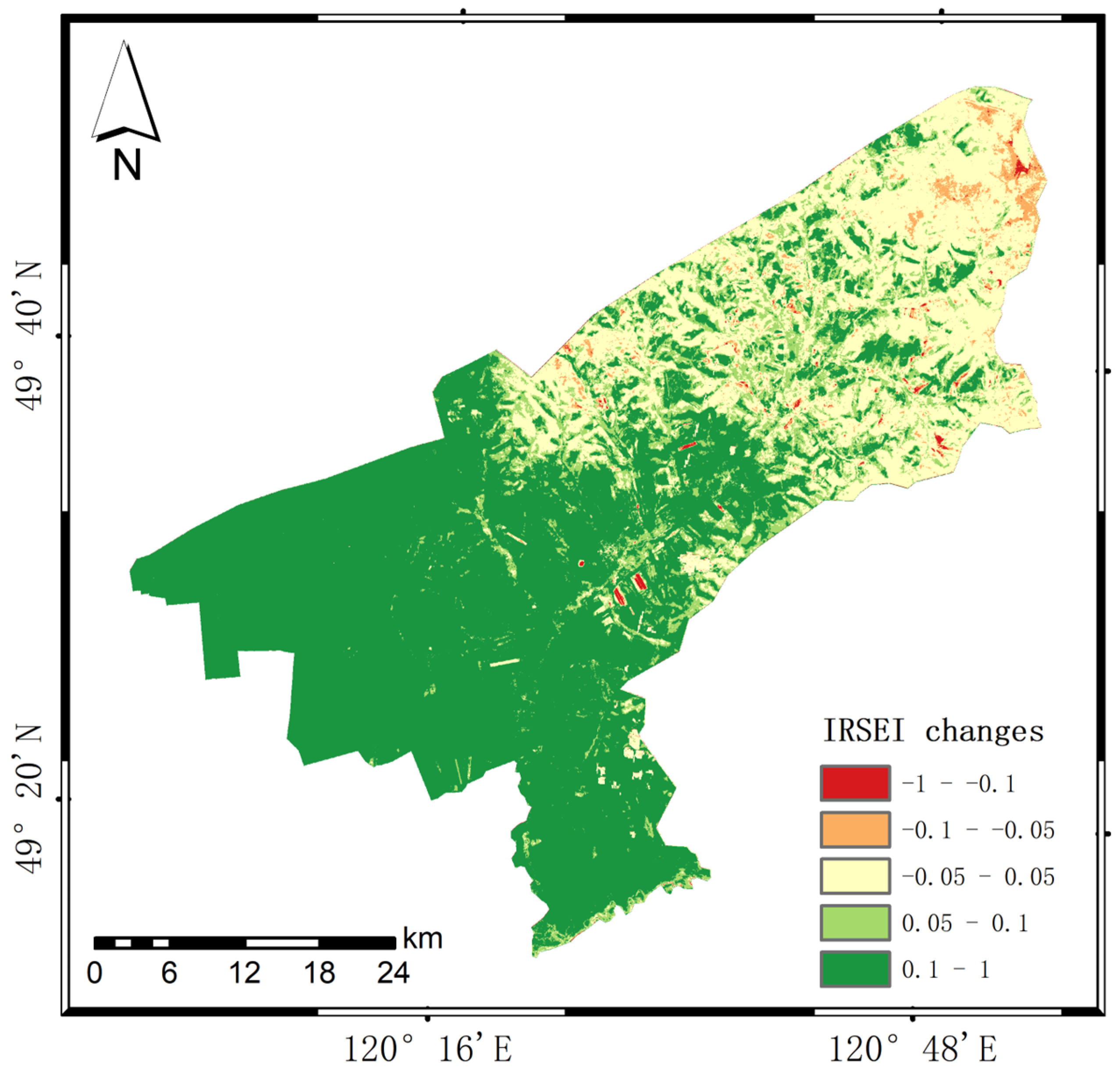
To further investigate the spatiotemporal variations in the IRSEI at Tenihe Farm, a differential calculation was conducted for the period spanning from 2013 to 2022, followed by stratified statistical analysis. The classification comprised five intervals, which were delineated as follows: significantly deteriorated (−1, −0.1), moderately deteriorated (−0.1, −0.05), essentially unchanged (−0.05, 0.05), moderately improved (0.05, 0.1), and significantly improved (0.1, 1). A visualization of the results is presented in Figure 11. Figure 11 clearly shows that, over the course of a decade, there have been alterations in the IRSEI, with some regions experiencing improvements in ecological environmental quality, while others have witnessed a decline.

The quantitative results of the temporal differentiation of the IRSEI at Tenihe Farm are presented in

Table 8. Analysis of changes in the IRSEI over a ten-year period at Tenihe Farm.

Changes	Index	(−1, −0.1)	(−0.1, −0.05)	(−0.05, 0.05)	(0.05, 0.1)	(0.1, 1]
2013–2022	Area/km2	7.79	44.52	501.29	267.10	1152.81
	Proportion/%	0.39	2.26	25.40	13.53	58.41

below. Table 8 reveals that, between 2013 and 2022, the most significant change in the ecological quality of Tenihe Farm was a marked improvement, encompassing an area of 1152.81 km², which constitutes 58.41% of the total area. This was followed by areas that remained essentially unchanged, covering 501.29 km², or 25.40% of the total area. Subsequently, areas that experienced a slight improvement accounted for 267.10 km², representing 13.53% of the total area. Areas with slight deterioration covered 44.52 km², comprising 2.26% of the total, while those that significantly deteriorated comprised 7.79 km², or 0.39% of the total area. It is evident that, over the course of the decade, the ecological quality of Tenihe Farm significantly improved, with only a minimal proportion of the area ecologically degrading. The combined percentage of areas that had slightly or significantly worsened was only 2.65%.

4.3. Comparative Analysis with the Original RSEI Method

4.3.1. Comparative Analysis of Different Land Use Types

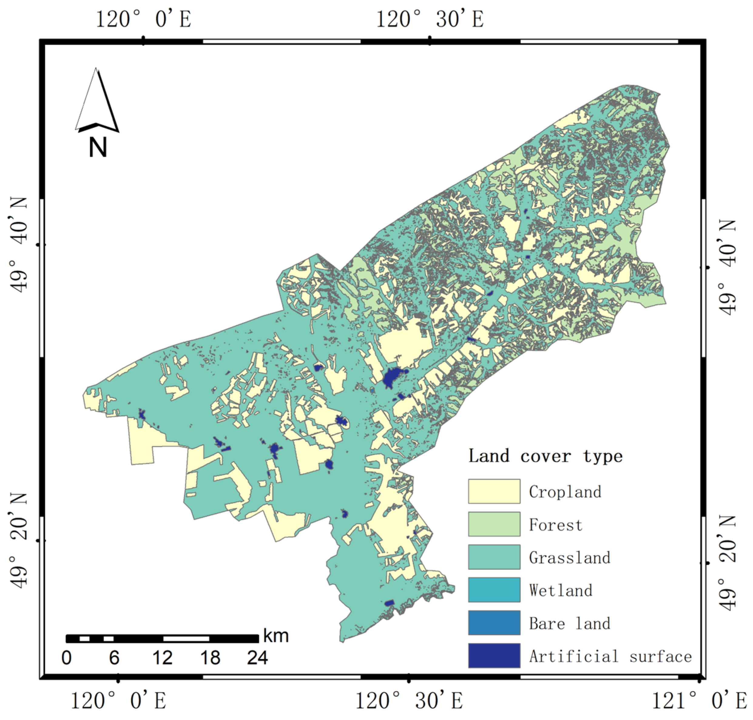
To further validate the efficacy of the IRSEI evaluation method proposed in this paper, we conducted a statistical analysis across different land use types. Given that the study area, Tenihe Farm, is a large-scale, intensively managed agricultural enterprise, the land use types have not changed over the span of a decade. Consequently, it is sufficient to categorize the land use types and perform a decadal statistical analysis of both the IRSEI and the RSEI within each category to clearly demonstrate the differences between the two ecological assessment methods. The land use type data were sourced from the farm management department. Following the creation of maps via ArcGIS 10.2, the land use types of Tenihe Farm can be identified, as shown in Figure 12.

The figure above illustrates that the land cover types of Tenihe Farm are predominantly categorized into six classifications: cropland, forest, grassland, wetland, bare land, and artificial surface. The statistical outcomes presented in the following table,

Table 9. Mean IRSEI and RSEI values for different feature cover types over a ten-year period.

Year	Index	Cropland	Forest	Grassland	Wetland	Bare Land	Artificial Surface
2013	IRSEI	0.4661	0.6538	0.4813	0.5370	0.3414	0.3396
	RSEI	0.4681	0.6134	0.5833	0.5579	0.4143	0.3956
2014	IRSEI	0.4586	0.7026	0.4731	0.5506	0.3449	0.3269
	RSEI	0.5173	0.6962	0.5245	0.5608	0.3963	0.3126
2015	IRSEI	0.4956	0.7057	0.4937	0.5716	0.3615	0.3455
	RSEI	0.5741	0.6713	0.5273	0.5492	0.3847	0.3131
2016	IRSEI	0.5325	0.7088	0.5143	0.5926	0.3780	0.3642
	RSEI	0.5783	0.5371	0.4849	0.6270	0.3836	0.3013
2017	IRSEI	0.5628	0.7330	0.5608	0.6120	0.3975	0.3264
	RSEI	0.6313	0.6051	0.5269	0.5794	0.4386	0.4049
2018	IRSEI	0.6064	0.7149	0.5554	0.6347	0.3112	0.3015
	RSEI	0.6501	0.7068	0.5751	0.6410	0.3676	0.3782
2019	IRSEI	0.6971	0.7876	0.6951	0.7028	0.3694	0.3882
	RSEI	0.7049	0.7853	0.6835	0.6595	0.3898	0.3894
2020	IRSEI	0.7879	0.8602	0.8348	0.7962	0.3297	0.3749
	RSEI	0.7927	0.8473	0.8015	0.7533	0.3324	0.3614
2021	IRSEI	0.7170	0.7660	0.7382	0.7630	0.3489	0.3567
	RSEI	0.7591	0.7805	0.7741	0.7231	0.3001	0.3621
2022	IRSEI	0.6462	0.6717	0.6516	0.6697	0.3680	0.3384
	RSEI	0.7060	0.6984	0.6874	0.6982	0.3585	0.3301

, were obtained by conducting a computational analysis of the IRSEI and RSEI results from 2013 to 2022 for each of the six land cover types.

Different land use types often exhibit distinctive ecological characteristics, and a meaningful and precise ecological quality assessment should align with the environmental features specific to these various land use categories. Within the study area addressed in this article, land cover types are primarily classified into six categories: cropland, forest, grassland, wetland, bare land, and artificial surface. Among these, grasslands may exhibit changes such as salinization due to factors such as grassland degradation, leading to potential instability in their ecological quality. Conversely, the ecological quality of forests and wetlands is expected to be superior to that of other types of forests. The ecological quality of cropland could surpass that of grasslands if scientific management practices are implemented; however, due to the impacts of activities such as fertilization and artificial planting, its ecological quality is unlikely to exceed that of forests and wetlands. Among the six categories, bare land and artificial surfaces are anticipated to have the lowest ecological quality. The data presented in the table corroborate the aforementioned ecological quality trends as reflected in the IRSEI. However, the RSEI results exhibit some deviations due to the omission of ecological characteristics such as soil salinization, as evidenced by the 2022 data in which croplands’ ecological quality was erroneously rated the highest among the six categories, which contradicts established ecological patterns. Therefore, we can infer that the IRSEI method proposed in this article offers a more accurate ecological assessment of the agricultural research area in question.

4.3.2. Comparative Analysis of the Correlation of the IRSEI and RSEI with Crop Yield

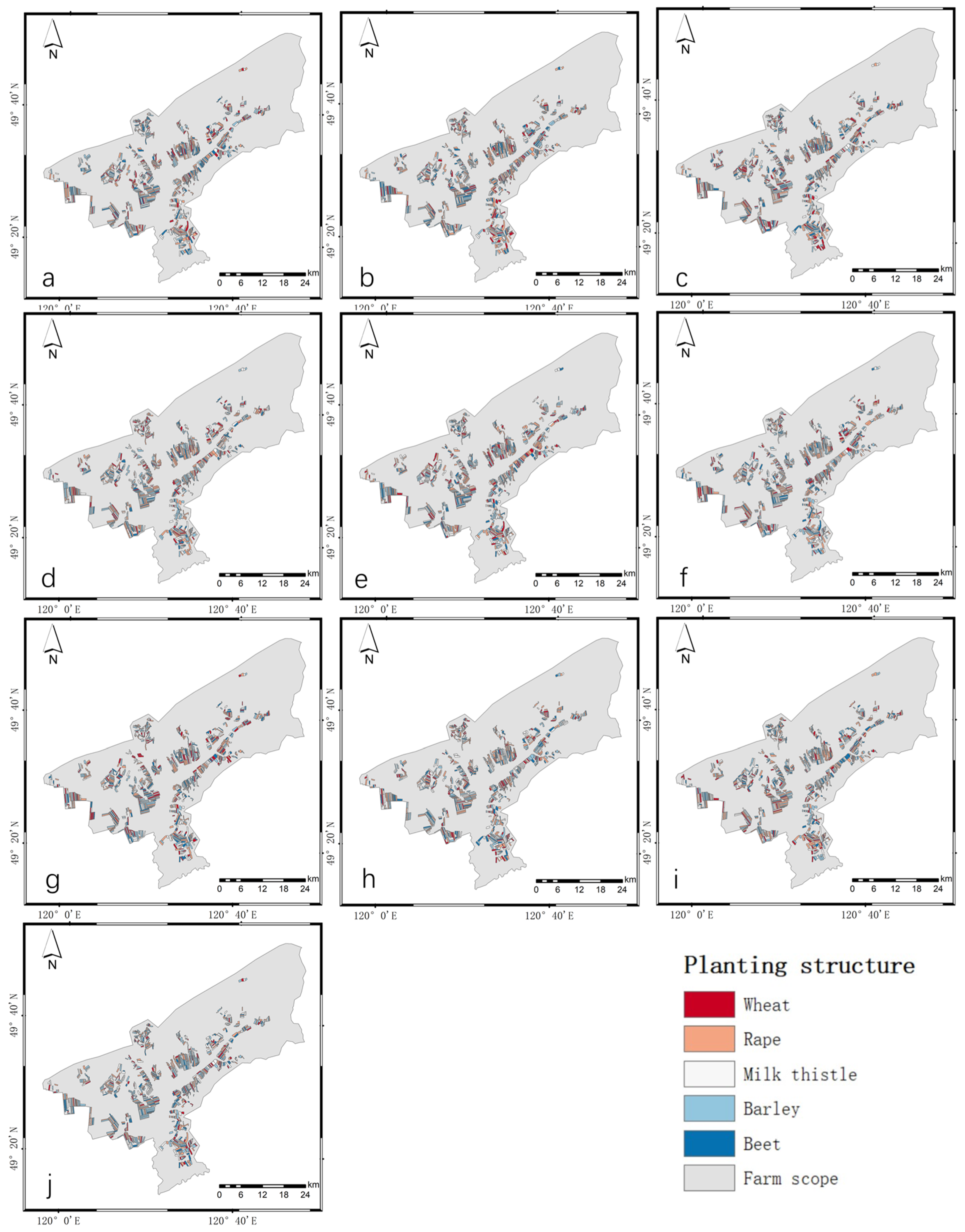
High-quality ecological conditions are a critical determinant of high crop yields; hence, the assessment of farmland ecological quality can, to some extent, reflect trend changes in crop yield. This paper conducted a comparative analysis of the correlation between the IRSEI method and the RSEI method with yield data to evaluate the effectiveness and accuracy of ecological quality assessments. Research revealed that Tenihe Farm adjusts the geographical locations of the types of crops planted annually. However, the overall crop types are categorized into five varieties, namely wheat, rape, milk thistle, barley, and beet. The composition and structure of the crop types over a decade are illustrated in Figure 13 below.

Prior to conducting a correlation analysis, it is imperative to acquire data on the yield of each crop over a span of ten years, which are furnished by the Department of Farm Management. This paper delineates a methodology to assess the correlation between two ecological quality evaluation outcomes and crop yields, as illustrated in

Table 10. Process for calculating the correlation of the IRSEI and RSEI with yield.

Input: IRSEI results, RSEI results, crop planting structure, the yield of each crop, and the extent of farmland.

Procedure: (1) Calculate the mean IRSEI and RSEI for each field unit. (2) Obtain statistics on the yield of field units based on crop classification (wheat, rape, milk thistle, barley, and beet). (3) Normalize the yield of crops by type, obtain five normalized results, and assign the results to the field units. (4) Use the PCC method to analyze the correlation between the IRSEI, the RSEI, and yield.

Output: The correlation results between the annual IRSEI and RSEI with the yield over the past decade.

below.

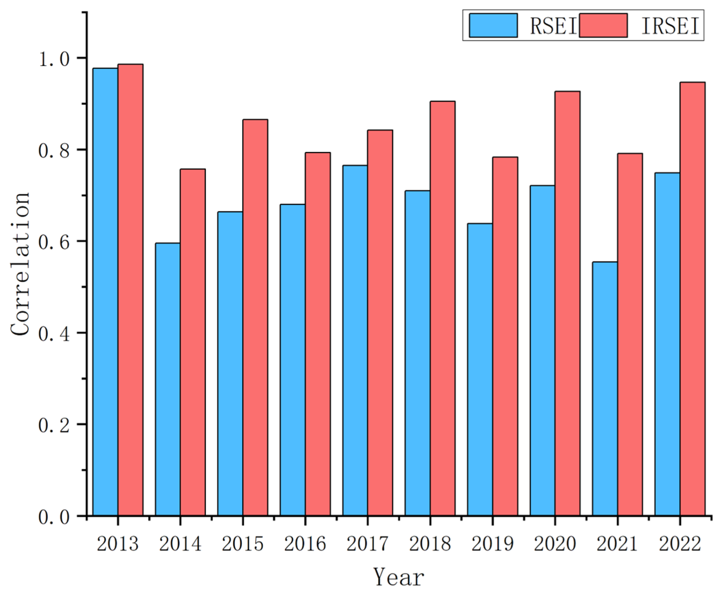
As shown in the table above, once the input data are prepared, the computational process for correlation primarily comprises four steps: The first step involves the calculation of IRSEI and RSEI values for the agricultural plots. The second step encompasses the compilation of yield data for five cultivated crops within these plots. The third step entails the normalization of the yield data for the five crops, with the standardized data laying the groundwork for subsequent correlation analysis. The fourth step is the computation of the correlation results. Following the procedural workflow and relevant computations, two sets of correlation outcomes between the IRSEI, RSEI, and crop yields over the decade from 2013 to 2022 were obtained. The results are depicted in Figure 14 below.

As can be inferred from Figure 14, over the decade from 2013 to 2022, the IRSEI exhibited a greater correlation with crop yields. Therefore, it can be deduced that the IRSEI method offers a higher degree of accuracy in evaluating the ecological quality of farms.

5. Discussion

This paper commenced from the perspective of the environmental characteristics present in semiarid agricultural planting regions with saline soils, and it constructed the IRSEI model to evaluate the temporal sequence of ecological quality in the farm study area. The model addressed the current state of soil salinization in the research area and proposed an integrated salinity index (ISI), which is a composite index derived from the amalgamation of three distinct salinity indices. The NDVI was used to represent the greenness component of the study area; the humidity component was characterized using the WET from the tasseled cap transformation, the dryness component was indicated with the NDBSI, a synthesis of the SI and the IBI, and the LST was utilized to denote the heat component. Through principal component transformation for the integration of component indicators, the normalized first principal component’s contribution rate exceeded 70%, effectively integrating the valid characteristic information of each indicator. Consequently, the generated IRSEI results proficiently represent the changes in the quality of the ecological environment of the farm within the study area.

To ensure the reliability of the data quality, a correlation analysis was conducted for the NDVI, WET, NDBSI, LST, and ISI indices with the IRSEI. The analysis revealed positive correlations between the greenness and humidity indices and the IRSEI and negative correlations between the dryness, heat, and salinity indices and the IRSEI. These results are consistent with the characteristic influences of ecological environmental factors, and they serve to validate the integrity of the data quality.

In the monitoring and assessment of ecological quality within a specific region, it is imperative to consider not only the commonly utilized indices within the RSEI framework, such as the greenness, humidity, dryness, and heat indices, but also unique ecological indicators pertinent to the study area. In the research presented in this paper, the study area was characterized by soil salinization. Consequently, we proposed an integrated salinity index (ISI) based on remote sensing to characterize the salinization trends of farms. This index was then integrated with the aforementioned four ecological indices to develop an improved remote sensing ecological index (IRSEI). A comparative analysis of the results between the IRSEI and RSEI outcomes was conducted, which was divided into two parts. The first part compared different land use types, with findings indicating that the IRSEI more accurately reflected the actual conditions across various land use categories, whereas the RSEI results deviated. The second part involved a correlation analysis between the IRSEI and RSEI results and the yield data of five different crops based on agricultural units. In comparison to the RSEI results, the IRSEI results demonstrated a stronger correlation with crop yield, thereby suggesting that the IRSEI more closely aligns with the growth trends of cultivated crops. This also, to a certain extent, underscores the precision advantage that IRSEI offers over RSEI.

The quality of the ecological environment in farming areas is a crucial component of food security. Only by ensuring the ecological integrity of farm regions can agricultural sustainability be guaranteed. In turn, sustainable agriculture can provide a green and healthy food source for human habitation. It can be argued that the quality of the ecological environment in crop cultivation areas is a vital foundation for the stable and healthy operation of the economy and society. Therefore, assessing farms’ ecological environment quality based on the IRSEI is highly important. Given that this method incorporates the ISI and considers the semiarid climate attributes of agricultural planting areas and the salinization characteristics of the soil, it has potential applicability and expansion potential in agricultural planting regions with soil salinization characteristics.

6. Conclusions

This paper has investigated the feasibility of the dynamic monitoring of ecological quality over time in semiarid agricultural planting areas characterized by soil salinization. An improved remote sensing ecological index, the IRSEI, was proposed, and spatial measurements and temporal evolution analyses of the ecological quality in the experimental area of Tenihe Farm were conducted based on objective remote sensing data. The IRSEI method was compared with the original RSEI method, revealing that the IRSEI performs more reliably across different land cover types. Compared to those of the RSEI method, the results produced using the IRSEI method have a greater correlation with the crop yields of the farm. These findings validate the effectiveness and increased accuracy of the proposed IRSEI method in assessing the ecological quality of salinized farms. Future research will consider other factors that contribute to changes in the ecological quality of agricultural planting areas, such as atmospheric conditions, precipitation, species diversity, and human activities, to more comprehensively evaluate the ecological quality of agricultural planting areas. Additionally, future work will explore the ecological quality of nonagricultural planting areas with soil salinization characteristics to test the generalizability of the proposed IRSEI method.

References

- Wu, D.; Jia, K.L.; Zhang, X.D.; Zhang, J.H.; Abd El Hamid, H.T. Remote Sensing Inversion for Simulation of Soil Salinization Based on Hyperspectral Data and Ground Analysis in Yinchuan, China. Nat. Resour. Res. 2021, 30, 4641–4656. [Google Scholar] [CrossRef]
- Singh, A. Soil salinization management for sustainable development: A review. J. Environ. Manag. 2021, 277, 111383. [Google Scholar] [CrossRef]
- Hatfield, S.B.I.A. Normalizing the stress-degree-day parameter for environmental variability. Agric. Meteorol. 1981, 24, 45–55. [Google Scholar]
- Wang, J.; Jiang, L.; Qi, Q.; Wang, Y. Exploration of semantic geo-object recognition based on the scale parameter optimization method for remote sensing images. Int. J. Geo Inf. 2021, 10, 420. [Google Scholar] [CrossRef]
- Gupta, K.; Kumar, P.; Pathan, S.K.; Sharma, K.P. Urban Neighborhood Green Index—A Measure of Green Spaces in Urban Areas. Landsc. Urban Plan. 2012, 105, 325–335. [Google Scholar] [CrossRef]
- Hengkai, L.; Feng, X.; Qin, L. Remote Sensing Monitoring of Land Damage and Restoration in Rare Earth Mining Areas in 6 Counties in Southern Jiangxi Based on Multisource Sequential Images. J. Environ. Manag. 2020, 267, 110653. [Google Scholar] [CrossRef]
- Crichton, K.A.; Anderson, K.; Charman, D.J.; Gallego-Sala, A. Seasonal climate drivers of peak NDVI in a series of Arctic peatlands. Sci. Total Environ. 2022, 838, 156419. [Google Scholar] [CrossRef]
- Piao, S.; Wang, X.; Park, T.; Chen, C.; Lian, X.; He, Y.; Bjerke, J.W.; Chen, A.; Ciais, P.; Tømmervik, H.; et al. Characteristics, drivers and feedbacks of global greening. Nat. Rev. Earth Environ. 2020, 1, 14–27. [Google Scholar] [CrossRef]
- Vernet, M.; Ellingsen, I.; Marchese, C.; Bélanger, S.; Cape, M.; Slagstad, D.; Matrai, P.A. Spatial variability in rates of net primary production (NPP) and onset of the spring bloom in Greenland shelf waters. Prog. Oceanogr. 2021, 198, 102655. [Google Scholar] [CrossRef]
- Moghimi, M.M.; Zarei, A.R.; Mahmoudi, M.R. Seasonal drought forecasting in arid regions, using different time series models and RDI index. J. Water Clim. Chang. 2020, 11, 633–654. [Google Scholar] [CrossRef]
- Xu, H.Q. A remote sensing urban ecological index and its application. Acta Ecol. Sin. 2013, 33, 7853–7862. [Google Scholar]
- Xu, H.; Wang, M.; Shi, T.; Guan, H.; Fang, C.; Lin, Z. Prediction of ecological effects of potential population and impervious surface increases using a remote sensing based ecological index (RSEI). Ecol. Indic. 2019, 93, 730–740. [Google Scholar] [CrossRef]
- Yuan, B.; Fu, L.; Zou, Y.; Zhang, S.; Chen, X.; Li, F.; Deng, Z.; Xie, Y. Spatiotemporal change detection of ecological quality and the associated affecting factors in Dongting Lake Basin, Based on RSEI. J. Clean. Prod. 2021, 302 (Suppl. S1), 126995. [Google Scholar] [CrossRef]
- Xu, H.; Fu, L.; Zou, Y.; Zhang, S.; Chen, X.; Li, F.; Deng, Z.; Xie, Y. Remote Sensing Detecting Ecological Changes with a Remote Sensing Based Ecological Index (RSEI) Produced Time Series and Change Vector Analysis. Remote Sens. 2019, 11, 2345. [Google Scholar] [CrossRef]
- Jing, Y.; Zhang, F.; He, Y.; Johnson, V.C.; Arikena, M. Assessment of spatial and temporal variation of ecological environment quality in Ebinur Lake Wetland National Nature Reserve, Xinjiang, China. Ecol. Indic. 2020, 110, 105874. [Google Scholar] [CrossRef]
- Qureshi, S.; Alavipanah, S.K.; Konyushkova, M.; Mijani, N.; Fathololomi, S.; Firozjaei, M.K.; Homaee, M.; Hamzeh, S.; Kakroodi, A.A. A Remotely Sensed Assessment of Surface Ecological Change over the Gomishan Wetland, Iran. Remote Sens. 2020, 12, 2989. [Google Scholar] [CrossRef]
- Liu, C.; Yang, M.; Hou, Y.; Zhao, Y.; Xue, X. Spatiotemporal evolution of island ecological quality under different urban densities: A comparative analysis of Xiamen and Kinmen Islands, southeast China. Ecol. Indic. 2021, 124, 107438. [Google Scholar] [CrossRef]
- Jiang, C.; Wu, L.; Liu, D.; Wang, S.M. Dynamic monitoring of eco-environmental quality in arid desert area by remote sensing: Taking the Gurbantunggut Desert China as an example. J. Appl. Ecol. 2019, 30, 877–883. [Google Scholar]
- Airiken, M.; Zhang, F.; Chan, N.W.; Kung, H.T. Assessment of spatial and temporal ecological environment quality under land use change of urban agglomeration in the North Slope of Tianshan, China. Environ. Sci. Pollut. Res. 2022, 29, 12282–12299. [Google Scholar] [CrossRef]
- Song, H.M.; Xue, L. Dynamic monitoring and analysis of ecological environment in Weinan City, Northwest China based on RSEI model. J. Appl. Ecol. 2016, 27, 3913. [Google Scholar]
- Nie, X.; Hu, Z.; Zhu, Q.; Ruan, M. Research on Temporal and Spatial Resolution and the Driving Forces of Ecological Environment Quality in Coal Mining Areas Considering Topographic Correction. Remote Sens. 2021, 13, 2815. [Google Scholar] [CrossRef]
- Xu, C.Y.; Li, B.W.; Kong, F.B.; He, T. Spatial-temporal variation, driving mechanism and management zoning of ecological resilience based on RSEI in a coastal metropolitan area. Ecol. Indic. 2024, 158, 111447. [Google Scholar] [CrossRef]
- Periasamy, S.; Shanmugam, R.S. Multispectral, Microwave Remote Sensing Models to Survey Soil Moisture and Salinity. Land Degrad. Dev. 2017, 28, 1412–1415. [Google Scholar] [CrossRef]
- Wu, W.; Bethel, M.; Mishra, D.R.; Hardy, T. Model selection in Bayesian framework to identify the best World View-2 based vegetation index in predicting green biomass of salt marshes in the northern Gulf of Mexico. GIScience Remote Sens. 2018, 55, 880–904. [Google Scholar] [CrossRef]
- Shrivastava, P.; Kumar, R. Soil salinity: A serious environmental issue and plant growth promoting bacteria as one of the tools for its alleviation. Saudi J. Biol. Sci. 2015, 22, 123–131. [Google Scholar] [CrossRef]
- Xiao, X.L.J. Soil salinization of cultivated land in Shandong Province, China-Dynamics during the past 40 years. Land Degrad. Dev. 2019, 30, 426–436. [Google Scholar] [CrossRef]
- Yang, J.S. Development and prospect of the research on salt-affected soils in China. Acta Pedol. Sin. 2008, 45, 837–845. [Google Scholar]
- Abuelgasim, A.; Ammad, R. Mapping soil salinity in arid and semi-arid regions using Landsat 8 OLI satellite data—ScienceDirect. Remote Sens. Appl. Soc. Environ. 2019, 13, 415–425. [Google Scholar]
- Kumar, N.; SSingh, K.; Pandey, H.K. Drainage morphometric analysis using open access earth observation datasets in a drought-affected part of Bundelkhand, India. Appl. Geomat. 2018, 10, 1–17. [Google Scholar] [CrossRef]
- Jun-Han, L.I.; Ming-Xiu, G. Temporal and Spatial Characteristics of Salinization of Coastal Soils in the Yellow River Delta. Chin. J. Soil Sci. 2018, 49, 1458–1465. [Google Scholar]
- Moran, M.S.; Clarke, T.R.; Inoue, Y.; Vidal, A. Estimating crop water deficit using the relation between surface-air temperature and spectral vegetation index. Remote Sens. Environ. 1994, 49, 246–263. [Google Scholar] [CrossRef]
- Ma, L.; Yin, G.; Zhou, Z.; Lu, H.; Li, M. Uncertainty of Object-Based Image Analysis for Drone Survey Images. In Drones—Application; IntechOpen: London, UK, 2018. [Google Scholar]
- Benz, U.C.; Hofmann, P.; Willhauck, G.; Lingenfelder, I.; Heynen, M. Multi-resolution, object-oriented fuzzy analysis of remote sensing data for GIS-ready information. ISPRS J. Photogramm. Remote Sens. 2004, 58, 239–258. [Google Scholar] [CrossRef]
- Yin, F.; Lewis, P.E.; Gómez-Dans, J.L. Bayesian atmospheric correction over land: Sentinel-2/MSI and Landsat 8/OLI, Geosci. Model Dev. 2022, 15, 7933–7976. [Google Scholar] [CrossRef]
- Sandholt, I.; Rasmussen, K.; Andersen, J. A simple interpretation of the surface temperature/vegetation index space for assessment of surface moisture status. Remote Sens. Environ. 2002, 79, 213–224. [Google Scholar] [CrossRef]
- Zhu, D.; Chen, T.; Wang, Z.; Niu, R. Detecting ecological spatial-temporal changes by Remote Sensing Ecological Index with local adaptability. J. Environ. Manag. 2021, 299, 113655. [Google Scholar] [CrossRef]
- Wang, S.; Huang, C.; Zhang, L.; Lin, Y.; Cen, Y.; Wu, T. Monitoring and Assessing the 2012 Drought in the Great Plains: Analyzing Satellite-Retrieved Solar-Induced Chlorophyll Fluorescence, Drought Indices, and Gross Primary Production. Remote Sens. 2016, 8, 61. [Google Scholar] [CrossRef]
- Saleh, S.K.; Amoushahi, S.; Gholipour, M. Spatiotemporal ecological quality assessment of metropolitan cities: A case study of central Iran. Environ. Monit. Assess. 2021, 193, 305. [Google Scholar] [CrossRef]
- Firozjaei, M.K.; Kiavarz, M.; Homaee, M.; Arsanjani, J.J.; Alavipanah, S.K. A novel method to quantify urban surface ecological poorness zone: A case study of several European cities. Sci. Total Environ. 2021, 757, 143755. [Google Scholar] [CrossRef]
- Rouse, J.W.; Haas, R.H.; Schell, J.A.; Deering, D.W. Monitoring Vegetation Systems in the Great Plains with Erts. NASA Spec. Publ. 1974, 351, 309. [Google Scholar]
- Roy, P.S.A. Rikimaru and S. Miyatake, Tropical forest cover density mapping. Trop. Ecol. 2002, 43, 39–47. [Google Scholar]
- Xu, H. A new index for delineating built-up land features in satellite imagery. Int. J. Remote Sens. 2008, 29, 4269–4276. [Google Scholar] [CrossRef]
- Huang, C.; Wylie, B.; Yang, L.; Homer, C.; Zylstra, G. Derivation of a tasseled cap transformation based on landsat 7 at-Satellite reflectance. Int. J. Remote Sens. 2002, 23, 1741–1748. [Google Scholar] [CrossRef]
- Zha, Y.; Gao, J.; Ni, S. Use of normalized difference built-up index in automatically mapping urban areas from TM imagery. Int. J. Remote Sens. 2003, 24, 583–594. [Google Scholar] [CrossRef]
- Xu, H. Analysis of Impervious Surface and its Impact on Urban Heat Environment using the Normalized Difference Impervious Surface Index (NDISI). Photogramm. Eng. Remote Sens. 2010, 76, 557–565. [Google Scholar] [CrossRef]
- Shivers, S.W.; Roberts, D.A.; Mcfadden, J.P. Using paired thermal and hyperspectral aerial imagery to quantify land surface temperature variability and assess crop stress within California orchards. Remote Sens. Environ. 2019, 222, 215–231. [Google Scholar] [CrossRef]
- Wulder, M.A.; Loveland, T.R.; Roy, D.P.; Crawford, C.J.; Masek, J.G.; Woodcock, C.E.; Allen, R.G.; Anderson, M.C.; Belward, A.S.; Cohen, W.B.; et al. Current status of Landsat program, science, and applications. Remote Sens. Environ. 2019, 225, 127–147. [Google Scholar] [CrossRef]
- Jimenez-Munoz, J.C.; Cristobal, J.; Sobrino, J.A.; Sòria, G.; Ninyerola, M.; Pons, X. Revision of the Single-Channel Algorithm for Land Surface Temperature Retrieval from Landsat Thermal-Infrared Data. IEEE Trans. Geosci. Remote Sens. 2009, 47, 339–349. [Google Scholar] [CrossRef]
- Jiménez-Muoz, J.C.; Sobrino, J.A. A generalized single-channel method for retrieving land surface temperature from remote sensing data (vol 109, art no D08112, 2004). J. Geophys. Res. Atmos. 2003, 108, 4688. [Google Scholar]
- Duan, S.B.; Li, Z.L.; Wang, C.; Zhang, S.; Tang, B.H.; Leng, P.; Gao, M.F. Land-surface temperature retrieval from Landsat 8 single-channel thermal infrared data in combination with NCEP reanalysis data and ASTER GED product. Int. J. Remote Sens. 2018, 40, 1763–1778. [Google Scholar] [CrossRef]
- Yan, L.; Roy, D.P. Spatially and temporally complete Landsat reflectance time series modelling: The fill-and-fit approach. Remote Sens. Environ. 2020, 241, 111718. [Google Scholar] [CrossRef]
- Wu, Z.C.; Ye, F.W.; Guo, F.S.; Liu, W.H.; Li, H.L.; Yang, Y. A Review on Application of Techniques of Principle Component Analysis on Extracting Alteration Information of Remote Sensing. J. Geo Inf. Sci. 2018, 20, 1644. [Google Scholar]
- Bannari, A.; El-Battay, A.; Bannari, R.; Rhinane, H. Sentinel-MSI VNIR and SWIR Bands Sensitivity Analysis for Soil Salinity Discrimination in an Arid Landscape. Remote Sens. 2018, 10, 855. [Google Scholar] [CrossRef]
- Scudiero, E.; Skaggs, T.H.; Corwin, D.L. Regional-scale soil salinity assessment using Landsat ETM+ canopy reflectance. Remote Sens. Environ. 2015, 169, 335–343. [Google Scholar] [CrossRef]
- Wang, J.; Ding, J.; Yu, D.; Ma, X.; Zhang, Z.; Ge, X.; Teng, D.; Li, X.; Liang, J.; Lizaga, I.; et al. Capability of Sentinel-2 MSI data for monitoring and mapping of soil salinity in dry and wet seasons in the Ebinur Lake region, Xinjiang, China. Geoderma. 2019, 353, 172–187. [Google Scholar] [CrossRef]
- Khan, N.M.; Rastoskuev, V.V.; Sato, Y.; Shiozawa, S. Assessment of hydrosaline land degradation by using a simple approach of remote sensing indicators. Agric. Water Manag. 2005, 77, 96–109. [Google Scholar] [CrossRef]
Figure 1.
Overview of Tenihe Farm.
Figure 2.
IRSEI-based process for evaluating the ecological quality of Tenihe Farm.
Figure 3.
Calculation process for land surface temperature.
Figure 4.
The greenness index results for the ecological environment assessment of Tenihe Farm: (a–j) correspond to the results from 2013 to 2022, respectively.
Figure 5.
The humidity index results for the ecological environment assessment of Tenihe Farm: (a–j) correspond to the results from 2013 to 2022, respectively.
Figure 6.
The dryness index results for the ecological environment assessment of Tenihe Farm: (a–j) correspond to the results from 2013 to 2022, respectively.
Figure 7.
The heat index results for the ecological environment assessment of Tenihe Farm: (a–j) correspond to the results from 2013 to 2022, respectively.
Figure 8.
The salinity index results for the ecological environment assessment of Tenihe Farm: (a–j) correspond to the results from 2013 to 2022, respectively.
Figure 9.
The means and standard deviations of the ecological assessment component indices of Tenihe Farm over the past decade.
Figure 10.
The IRSEI results for the ecological environment assessment of Tenihe Farm: (a–j) correspond to the results from 2013 to 2022, respectively.
Figure 11.
Changes in the IRSEI over ten years according to the ecological environment assessment of Tenihe Farm.
Figure 12.
Land cover types of Tenihe Farm.
Figure 13.
Crop types and spatial distribution of crops grown on Tenihe Farm over a ten-year period: (a–j) correspond to the results from 2013 to 2022, respectively.
Figure 14.
Correlation results between the ecological quality evaluation and yield at Tenihe Farm.