
Fusion Method of RFI Detection, Localization, and Suppression by Combining One-Dimensional and Two-Dimensional Synthetic Aperture Radiometers
Abstract
:1. Introduction
2. Related Work of the RFI Detection, Localization, and Mitigation of Single Payload
2.1. RFI Detection and Localization
2.2. RFI Mitigation
2.3. Summary
3. Foundation
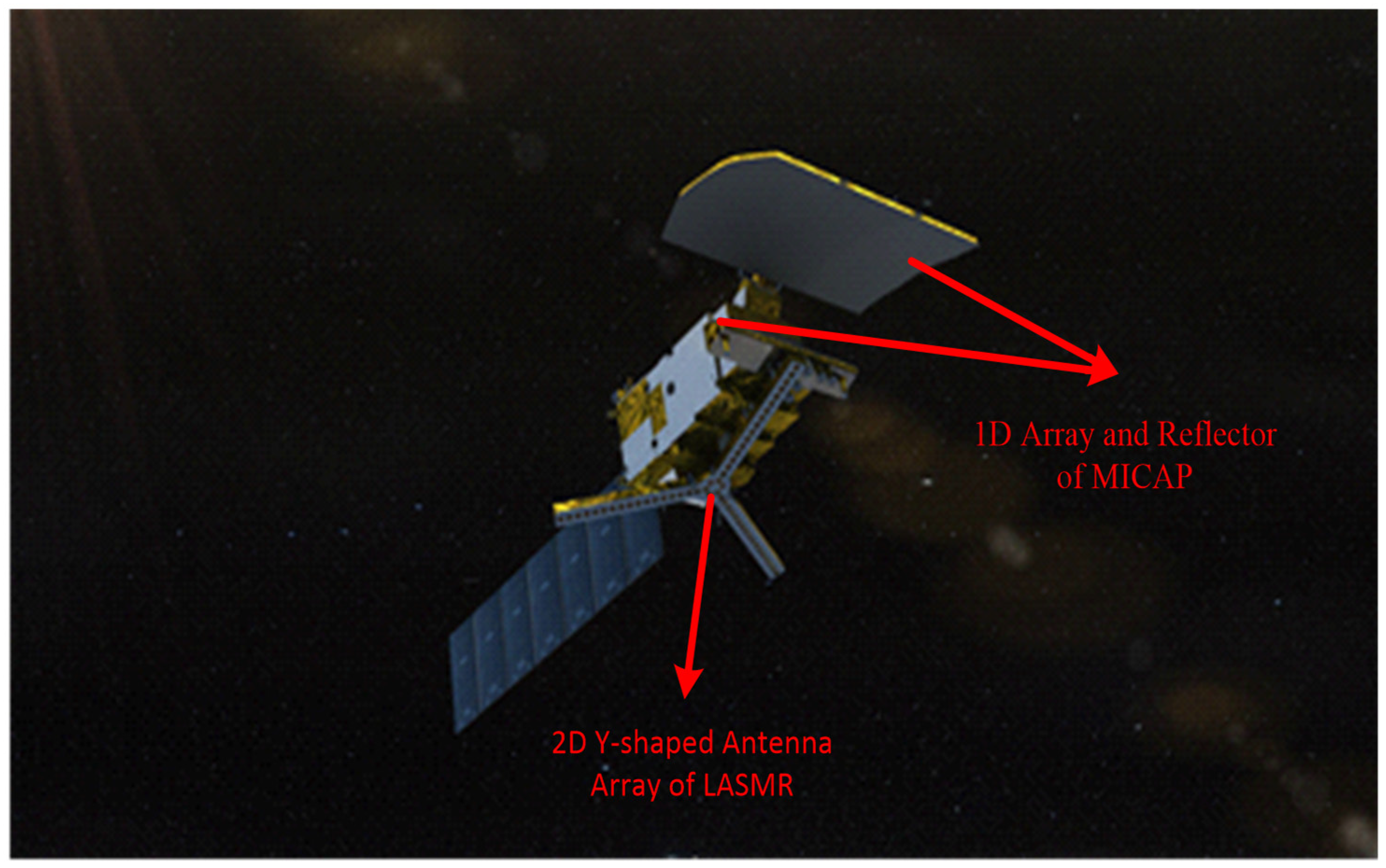
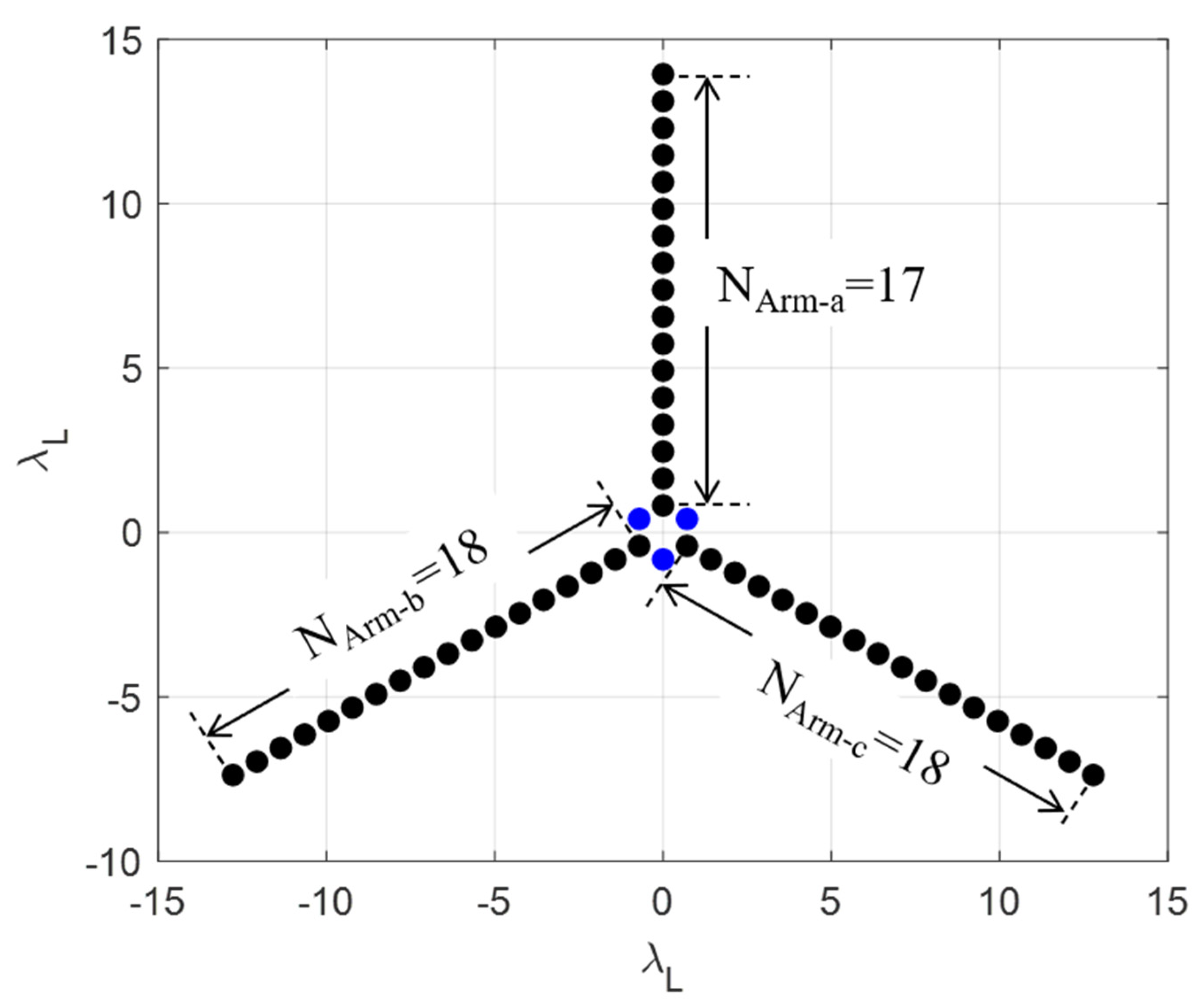
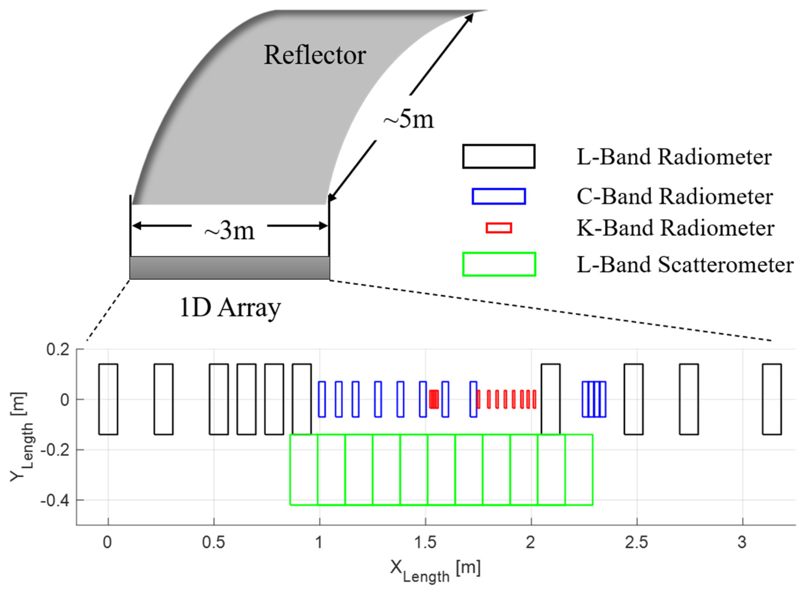
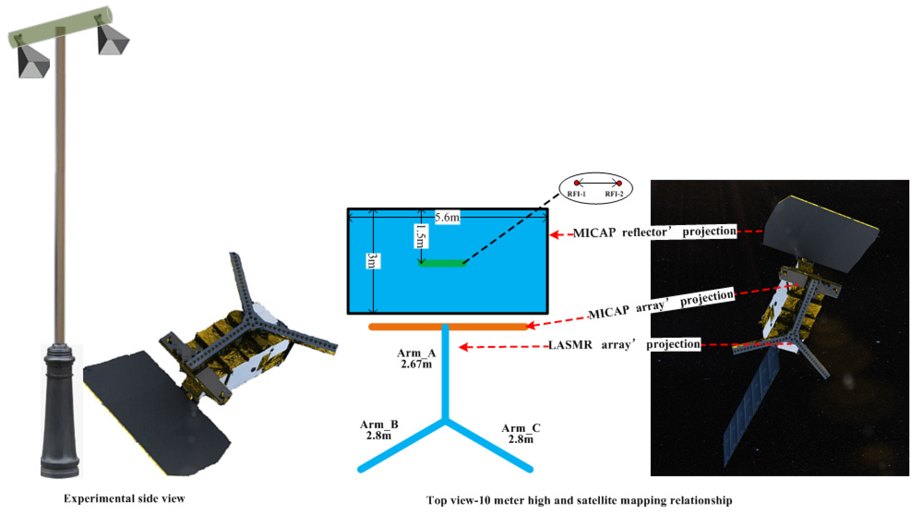
3.1. Satellite and Payload Description
3.2. Theory of Interferometric Radiometer
4. Experiment Settings
4.1. System Configuration
4.2. Input Data
4.3. Verification Data
5. Method
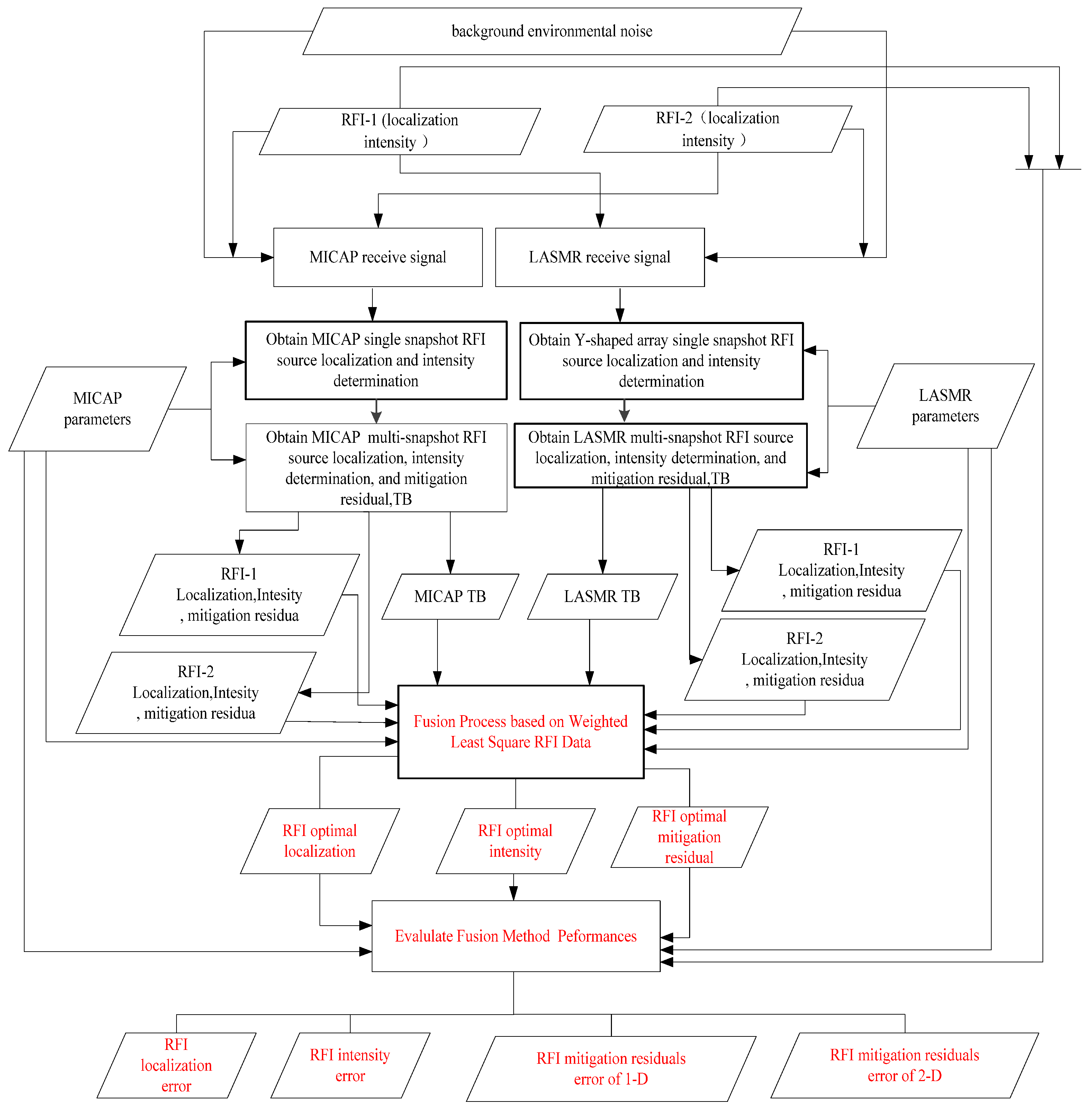
5.1. Fusion Method Overview
5.2. Fusion Method Based on Weighted Least Square Principle
5.3. Fusion Method Performance Evaluation
5.4. Fusion Method Steps and Verification Process
6. Results and Analysis
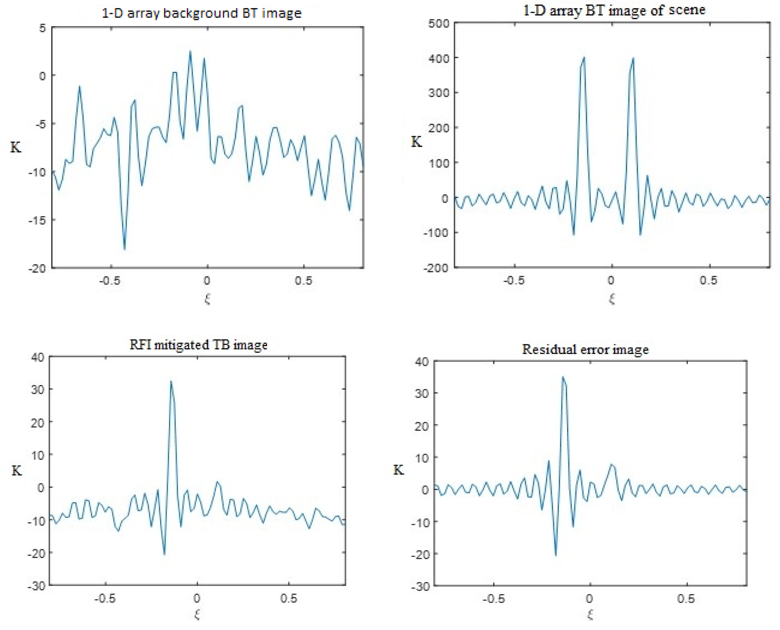
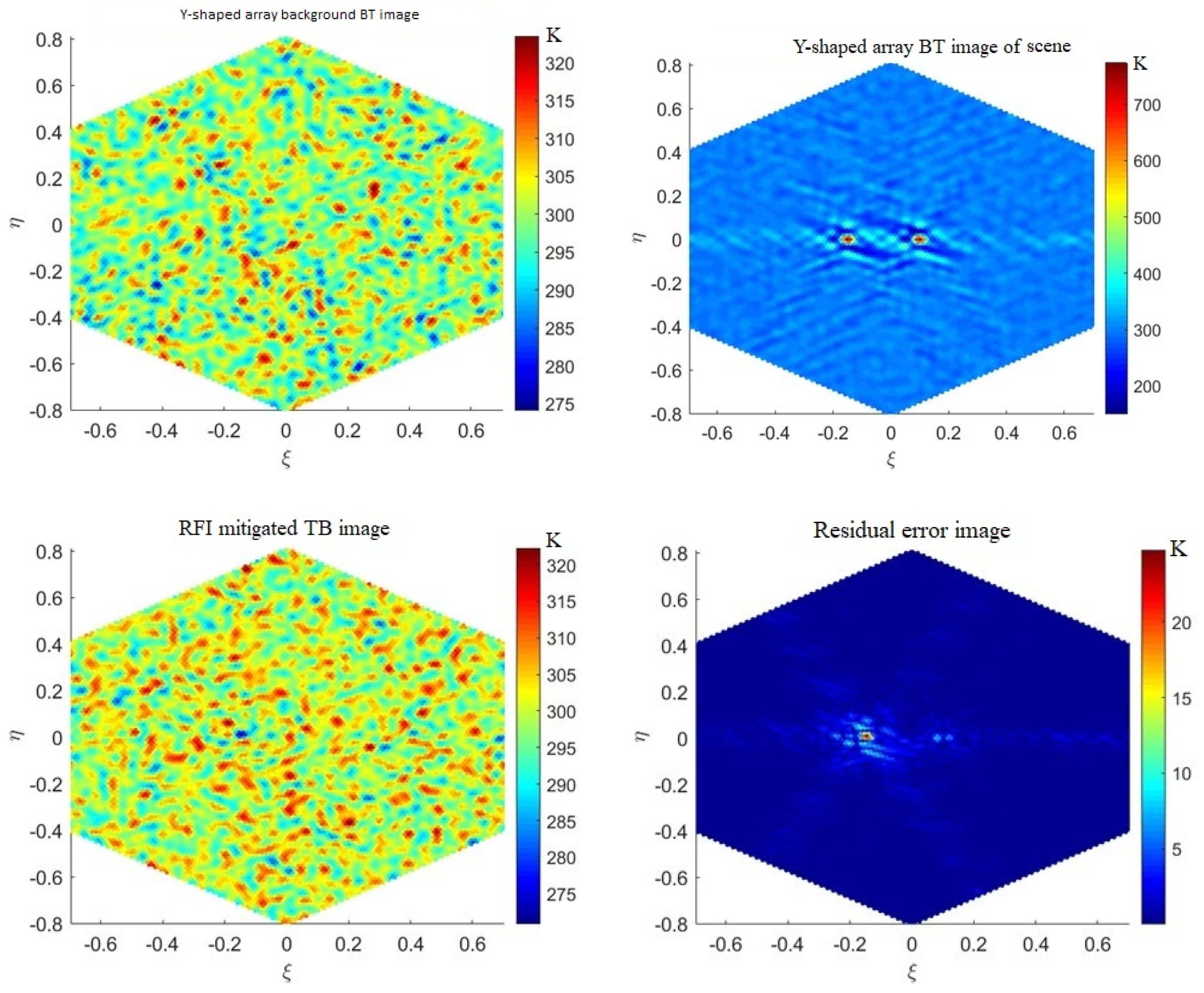
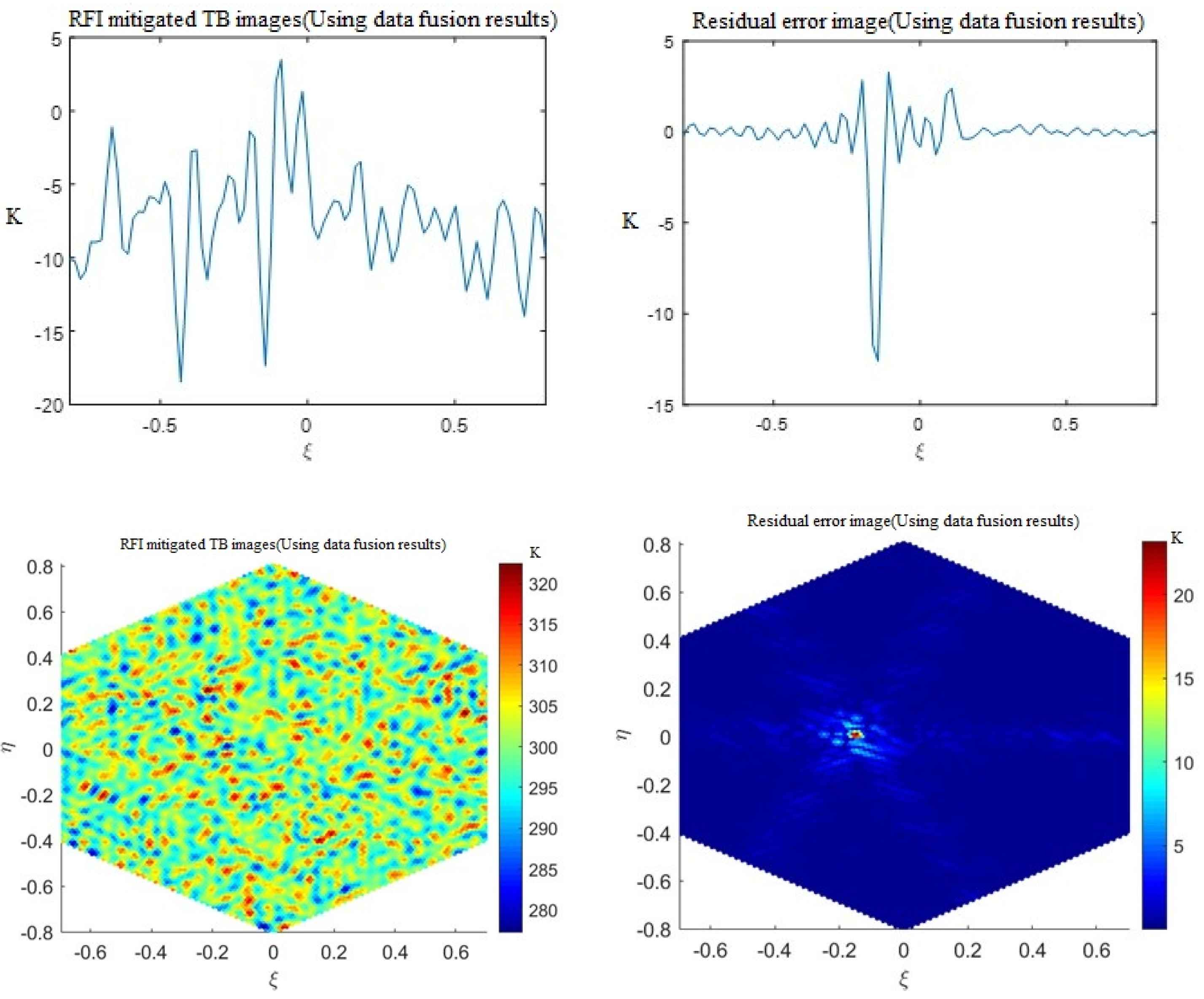
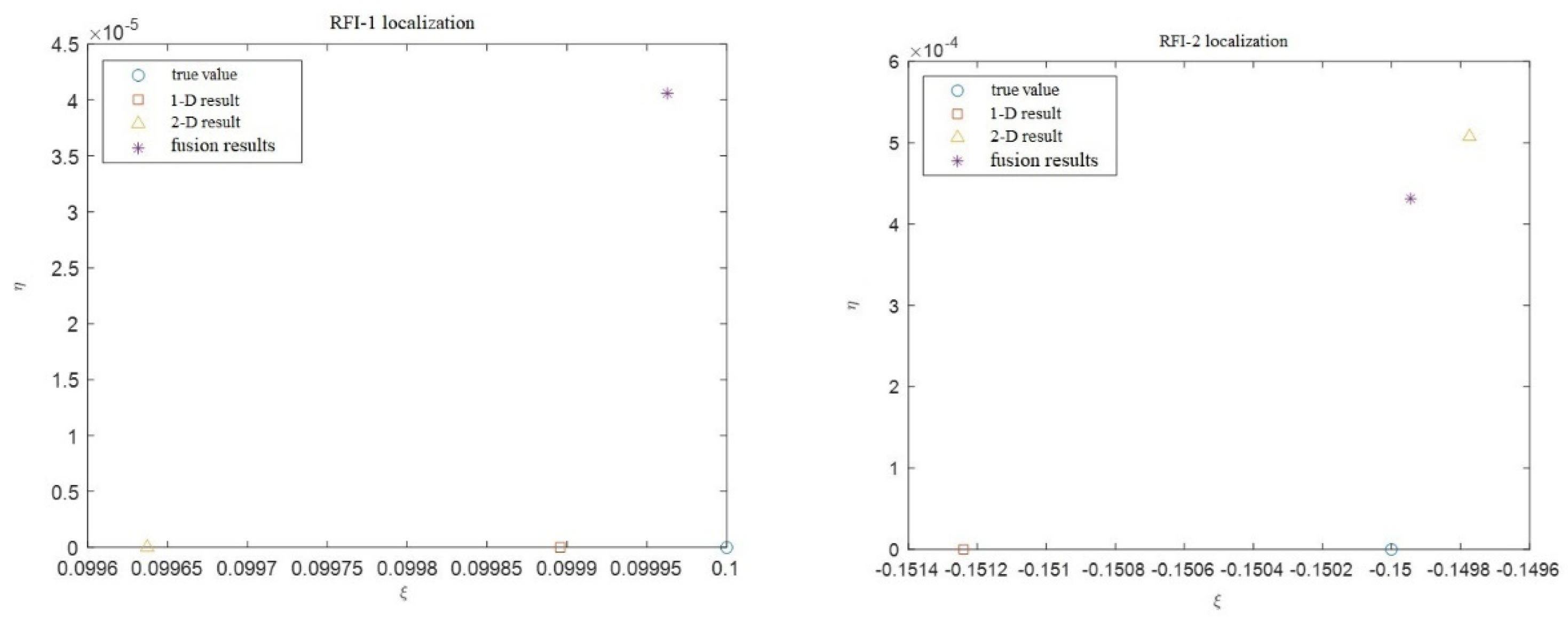
6.1. Results
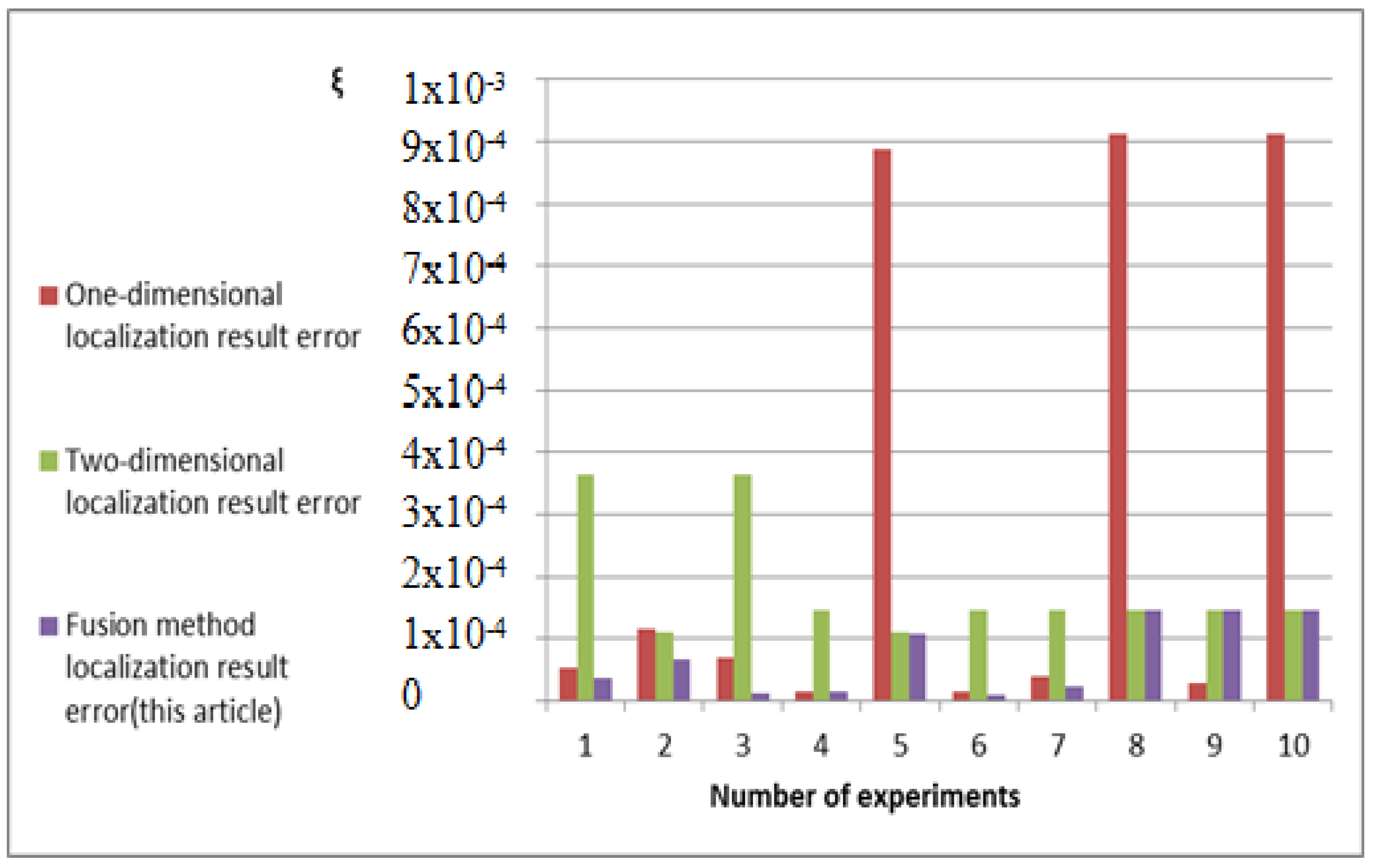
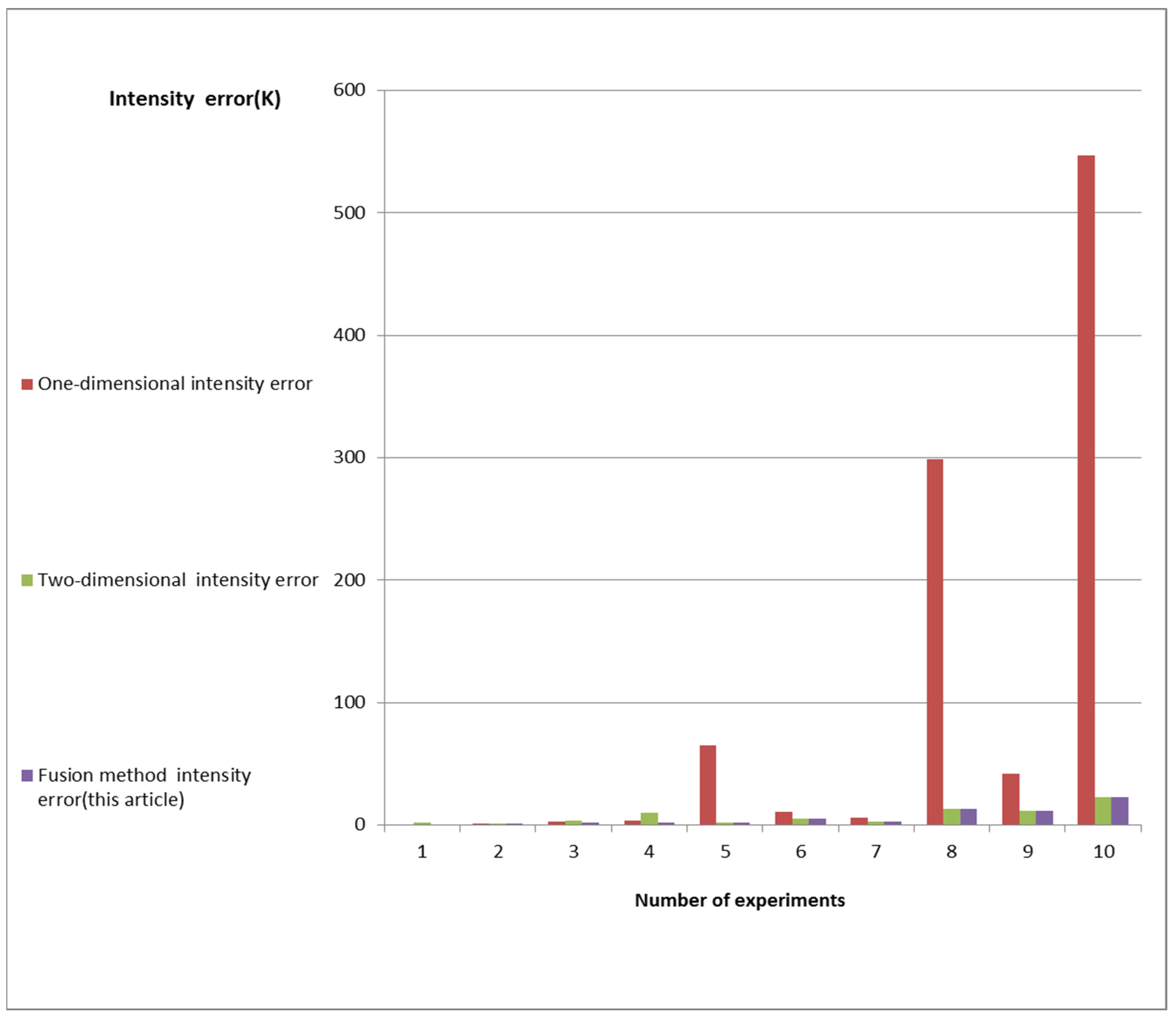
6.2. Comparison and Verification
7. Conclusions
Author Contributions
Funding
Data Availability Statement
Acknowledgments
Conflicts of Interest
References
- Zhang, Q.; Zhang, L.; Jia, Y.; Wang, B.; Li, S. Development and Prospect of Satellite Remote Sensing Technology for Ocean Dynamic Environment. J. Spacecr. Rocket. 2023, 60, 1679–1698. [Google Scholar] [CrossRef]
- Song, X.; Cui, X.; Zhai, Y.; Yan, J.; Duan, Z. Remote Sensing of Sea Surface Salinity and Temperature with Microwave Radiometers Research Review. Spacecr. Eng. 2021, 30, 108–114. [Google Scholar]
- Zhang, Q.; Yin, X.; Jiang, Y. Developing Sea Surface Salinity Satellite to Promote Ocean Dynamical Enviroments Observation. Spacecr. Eng. 2017, 26, 1–5. [Google Scholar] [CrossRef]
- Dinnat, E.P.; Le Vine, D.M.; Boutin, J.; Meissner, T.; Lagerloef, G. Remote Sensing of Sea Surface Salinity: Comparison of Satellite and In Situ Observations and Impact of Retrieval Parameters. Remote Sens. 2019, 11, 750. [Google Scholar] [CrossRef]
- Font, J.; Camps, A.; Borges, A.; Martin-Neira, M.; Boutin, J.; Reul, N.; Kerr, Y.H.; Hahne, A.; Mecklenburg, S. SMOS: The Challenging Sea Surface Salinity Measurement from Space. Proc. IEEE 2010, 98, 649–665. [Google Scholar] [CrossRef]
- Llorente, A.; Daganzo, E.; Oliva, R.; Uranga, E.; Kerr, Y.; Richaume, P.; de la Fuente, A.; Martin-Neira, M.; Mecklenburg, S. Lessons learnt from SMOS RFI activities after 10 years in orbit: RFI detection and reporting to claim protection and increase awareness of the interference problem in the 1400–1427 MHz passive band. In Proceedings of the RFI Workshop-Coexisting Radio Frequency Interference (RFI), Toulouse, France, 23–26 September 2019; pp. 1–6. [Google Scholar] [CrossRef]
- Skou, N.; Balling, J.E.; Søbjærg, S.S.; Kristensen, S.S. Surveys and analysis of RFI in the SMOS context. In Proceedings of the IEEE International Geoscience and Remote Sensing Symposium, Honolulu, HI, USA, 25–30 July 2010; pp. 2011–2014. [Google Scholar] [CrossRef]
- Uranga, E.; Llorente, A.; Oliva, R.; de la Fuente, A.; Daganzo, E.; Kerr, Y. Monitoring of SMOS RFI sources in the 1400–1427 MHz passive band. In Proceedings of the IGARSS 2018—2018 IEEE International Geoscience and Remote Sensing Symposium, Valencia, Spain, 22–27 July 2018; pp. 1241–1244. [Google Scholar] [CrossRef]
- Martín-Neira, M.; Oliva, R.; Corbella, I.; Torres, F.; Duffo, N.; Durán, I.; Kainulainen, J.; Closa, J.; Zurita, A.; Cabot, F.; et al. Lessons learnt from SMOS after 7 years in orbit. In Proceedings of the IEEE International Geoscience & Remote Sensing Symposium, Fort Worth, TX, USA, 23–28 July 2017. [Google Scholar] [CrossRef]
- Bringer, A.; Johnson, J.T.; Mohammed, P.N.; Misra, S.; Vine, D.L. Monitoring The L-Band RFI Environment: Tracking RFI Sources Observed by Smap. In Proceedings of the 2022 IEEE International Geoscience and Remote Sensing Symposium, IGARSS 2022, Kuala Lumpur, Malaysia, 17–22 July 2022; pp. 4240–4243. [Google Scholar] [CrossRef]
- de Matthaeis, P.; Le Vine, D. RFI detection and mitigation for Aquarius: Status and ongoing improvements. In Proceedings of the URSIGASS 2014, Beijing, China, 16–23 August 2014; pp. 1–3. [Google Scholar] [CrossRef]
- Li, Y.; Yin, X.; Zhou, W.; Lin, M.; Liu, H.; Li, Y. Performance Simulation of the Payload IMR and MICAP Onboard the Chinese Ocean Salinity Satellite. IEEE Trans. Geosci. Remote Sens. 2022, 60, 5301916. [Google Scholar] [CrossRef]
- Li, Y.; Yin, X.; Zhou, W.; Lin, M.; Ma, C.; Jin, R.; Liu, H.; Li, Y. Simulation Analysis of Payload IMR and MICAP Onboard Chinese Ocean Salinity Satellite. In Proceedings of the IGARSS 2020—2020 IEEE International Geoscience and Remote Sensing Symposium, Waikoloa, HI, USA, 26 September–2 October 2020; pp. 5635–5638. [Google Scholar] [CrossRef]
- Bin, L.; Dong, Z.; Fei, H. An improved RFI source detection method based on array factor property for synthetic aperture interferometric radiometer. In Proceedings of the SPIE, Microwave Remote Sensing: Data Processing and Applications II, Amsterdam, The Netherlands, 3–7 September 2023; Volume 12732, p. 1273206. [Google Scholar] [CrossRef]
- Jin, R.; Li, Q.; Liu, H. A Subspace Algorithm to Mitigate Energy Unknown RFI for Synthetic Aperture Interferometric Radiometer. IEEE Trans. Geosci. Remote Sens. 2020, 58, 227–237. [Google Scholar] [CrossRef]
- Oliva, R.; Nieto, S.; Felix, F. RFI detection algorithm: Accurate geolocation of the interfering sources in SMOS images. In Proceedings of the IEEE International Geoscience and Remote Sensing Symposium (IGARSS), Munich, Germany, 22–27 July 2012; pp. 3324–3326. [Google Scholar]
- Oliva, R.; Nieto, S.; Felix, F. RFI Detection Algorithm: Accurate Geolocation of the Interfering Sources in SMOS Images. IEEE Trans. Geosci. Remote Sens. 2013, 51, 4993–4998. [Google Scholar] [CrossRef]
- Castro, R.; Gutierrez, A.; Barbosa, J. A first set of techniques to detect radio frequency interferences and mitigate their impact on SMOS data. IEEE Trans. Geosci. Remote Sens. 2012, 50, 1440–1447. [Google Scholar] [CrossRef]
- Soldo, Y.; Cabot, F.; Khazaal, A.; Miernecki, M.; Słomińska, E.; Fieuzal, R.; Kerr, Y.H. Localization of RFI Sources for the SMOS Mission A Means for Assessing SMOS Pointing Performances. IEEE J. Sel. Top. Appl. Earth Obs. Remote Sens. 2015, 8, 617–627. [Google Scholar] [CrossRef]
- Park, H.; González-Gambau, V.; Camps, A.; Vall-Llossera, M. Improved MUSIC-Based SMOS RFI Source Detection and Geolocation Algorithm. IEEE Trans. Geosci. Remote Sens. 2016, 54, 1311–1322. [Google Scholar] [CrossRef]
- Li, J.; Hu, F.; He, F.; Wu, L. High-resolution RFI localization using covariance matrix augmentation in synthetic aperture interferometric radiometry. IEEE Trans. Geosci. Remote Sens. 2018, 56, 1186–1198. [Google Scholar] [CrossRef]
- Zhu, D.; Peng, X.; Li, G. A Matrix Completion Based Method for RFI Source Localization in Microwave Interferometric Radiometry. IEEE Trans. Geosci. Remote Sens. 2021, 59, 7588–7602. [Google Scholar] [CrossRef]
- Li, J.; Hu, F.; He, F.; Wu, L.; Peng, X.; Cheng, Y.; Zhu, D.; Chen, K. Super-resolution RFI localization with compressive sensing in synthetic aperture interferometric radiometers. In Proceedings of the IEEE International Geoscience and Remote Sensing Symposium (IGARSS), Milan, Italy, 26–31 July 2015; pp. 4734–4737. [Google Scholar] [CrossRef]
- Zhu, D.; Li, J.; Li, G. RFI Source Localization in Microwave Interferometric Radiometry: A Sparse Signal Reconstruction Perspective. IEEE Trans. Geosci. Remote Sens. 2020, 58, 4006–4017. [Google Scholar] [CrossRef]
- Camps, A.; Vall-Llossera, M.; Duffo, N.; Zapata, M.; Corbella, I.; Torres, F.; Barrena, V. Sun effects in 2-D aperture synthesis radiometry imaging and their cancelation. IEEE Trans. Geosci. Remote Sens. 2004, 42, 1161–1167. [Google Scholar] [CrossRef]
- Camps, A.; Bará, J.; Torres, F.; Corbella, I. Extension of the CLEAN technique to the microwave imaging of continuous thermal sources by means of aperture synthesis radiometers. J. Electromagn. Waves Appl. 1998, 12, 311–313. [Google Scholar] [CrossRef]
- Soldo, Y.; Khazaal, A.; Cabot, F.; Anterrieu, E.; Richaume, P. RFI mitigation for SMOS: A distributed approach. In Proceedings of the IEEE International Geoscience and Remote Sensing Symposium (IGARSS), Munich, Germany, 22–27 July 2012; pp. 3327–3330. [Google Scholar] [CrossRef]
- Soldo, Y.; Khazaal, A.; Cabot, F.; Richaume, P.; Anterrieu, E.; Kerr, Y.H. Mitigation of RFIs for SMOS: A Distributed Approach. IEEE Trans. Geosci. Remote Sens. 2014, 52, 7470–7479. [Google Scholar] [CrossRef]
- Hu, F.; Peng, X.; He, F.; Wu, L.; Li, J.; Cheng, Y.; Zhu, D. RFI Mitigation in Aperture Synthesis Radiometers Using a Modified CLEAN Algorithm. IEEE Geosci. Remote Sens. Lett. 2017, 14, 13–17. [Google Scholar] [CrossRef]
- Peng, X.; Hu, F.; He, F.; Zhu, D.; Cheng, Y.; Hu, H.; Zheng, T. An improved CLEAN algorithm for RFI Mitigation in Aperture Synthesis Radiometers. In Proceedings of the IEEE International Geoscience and Remote Sensing Symposium (IGARSS), Fort Worth, TX, USA, 23–28 July 2017; pp. 3448–3451. [Google Scholar] [CrossRef]
- Li, J.; Hu, F.; He, F.; Wu, L.; Peng, X. SMOS RFI mitigation using array factor synthesis of synthetic aperture interferometric radiometry. In Proceedings of the IEEE International Geoscience and Remote Sensing Symposium (IGARSS), Beijing, China, 10–15 July 2016; pp. 820–823. [Google Scholar] [CrossRef]
- Camps, A.; Park, H.; González-Gambau, V. An imaging algorithm for synthetic aperture interferometric radiometers with built-in RFI mitigation. In Proceedings of the IEEE Specialist Meeting on Microwave Radiometry and Remote Sensing of the Environment (MicroRad), Pasadena, CA, USA, 24–27 March 2014; pp. 39–43. [Google Scholar] [CrossRef]
- Li, J.; Hu, F.; He, F.; Wu, L.; Peng, X.; Zhu, D. An Imaging Method With Array Factor Synthesis in Synthetic Aperture Interferometric Radiometers. IEEE Geosci. Remote Sens. Lett. 2016, 13, 87–91. [Google Scholar] [CrossRef]
- Peng, X.; Hu, F.; He, F.; Wu, L.; Li, J.; Zhu, D.; Liao, Z.; Qian, C. RFI Mitigation of SMOS image based on CLEAN Algorithm. In Proceedings of the IEEE International Geoscience and Remote Sensing Symposium (IGARSS), Beijing, China, 10–15 July 2016; pp. 816–819. [Google Scholar] [CrossRef]
- Li, Y.; Zhang, W.; Zhang, J.; Zhang, L. Improved CLEAN Algorithm for RFI Mitigation of Aperture Synthesis Radiometer Images. IEEE Geosci. Remote Sens. Lett. 2022, 19, 4018105. [Google Scholar] [CrossRef]
- Li, Y.; Lin, M.; Yin, X.; Zhou, W. Analysis of the Antenna Array Orientation Performance of the Interferometric Microwave Radiometer (IMR) Onboard the Chinese Ocean Salinity Satellite. Sensors 2020, 20, 5396. [Google Scholar] [CrossRef] [PubMed]
- Liu, H.; Zhu, D.; Niu, L.; Wu, L.; Wang, C.; Chen, X.; Zhao, X.; Zhang, C.; Zhang, X.; Yin, X.; et al. MICAP (Microwave imager combined active and passive): A new instrument for Chinese ocean salinity satellite. In Proceedings of the 2015 IEEE International Geoscience and Remote Sensing Symposium (IGARSS), Milan, Italy, 26–31 July 2015; pp. 184–187. [Google Scholar] [CrossRef]
- Soldo, Y.; Le Vine, D.M. Characteristics of the RFI Environment at L-Band as Observed from SMAP; No. NASA/TM-20210000962; NASA: Washington, DC, USA, 2021. [Google Scholar]
- Corbella, I.; Duffo, N.; Vall-Llossera, M.; Camps, A.; Torres, F. The visibility function in interferometric aperture synthesis radiometry. IEEE Trans. Geosci. Remote Sens. 2004, 42, 1677–1682. [Google Scholar] [CrossRef]
- Gao, Y.; Zhou, W.; Zhang, L.; Zhang, H.; Jin, R.; Li, Q. A Combined RFI Localization Algorithm of BT Image and Subspace Decomposition for Synthetic Aperture Interferometric Radiometer. IEEE Trans. Geosci. Remote Sens. 2023, 61, 5301311. [Google Scholar] [CrossRef]
- Xu, Y.; Zhu, D.; Hu, F.; Fu, P. RFI Localization Using Jointly Non-Convex Low-Rank Approximation and Expanded Virtual Array in Microwave Interferometric Radiometry. IEEE Trans. Geosci. Remote Sens. 2023, 61, 5300515. [Google Scholar] [CrossRef]
- Park, H.; Camps, A. Accurate geolocation of RFI sources in SMOS imagery based on superresolution algorithms. In Proceedings of the IEEE Specialist Meeting on Microwave Radiometry and Remote Sensing of the Environment (MicroRad), Pasadena, CA, USA, 24–27 March 2014; pp. 29–32. [Google Scholar] [CrossRef]


| Index | LASMR | MICAP |
|---|---|---|
| Frequency | 1.4 GHz | 1.4 GHz |
| Bandwidth | 20 MHz | 25 MHz |
| Antenna | 2D, Y-shaped | 1D array + reflector |
| Number of elements | 56 | 12 |
| Minimum spacing | 0.82 | 0.61 |
| Effective integral time (τeff) | 0.9 s/2.46 | 0.9 s/1.51 |
| Filter factor (Ωα) | 1.7 | 1 |
| Window function (αw) | Blackman window, 0.45 | |
| Local oscillator | Double sideband, 1 | |
| Receiver noise temperature | 140 K | 233 K |
| Instrument stability per month | 0.12 K | 0.12 K |
| Number | RFI-1 Intensity | RFI-2 Intensity |
|---|---|---|
| 1. | A (450 K) | A (450 K) |
| 2. | A (450 K) | B (1200 K) |
| 3. | A (450 K) | C (5500 K) |
| 4. | A (450 K) | D (10,000 K) |
| 5. | B (1200 K) | B (1200 K) |
| 6. | B (1200 K) | C (5500 K) |
| 7. | B (1200 K) | D (10,000 K) |
| 8. | C (5500 K) | C (5500 K) |
| 9. | C (5500 K) | D (10,000 K) |
| 10. | D (10,000 K) | D (10,000 K) |
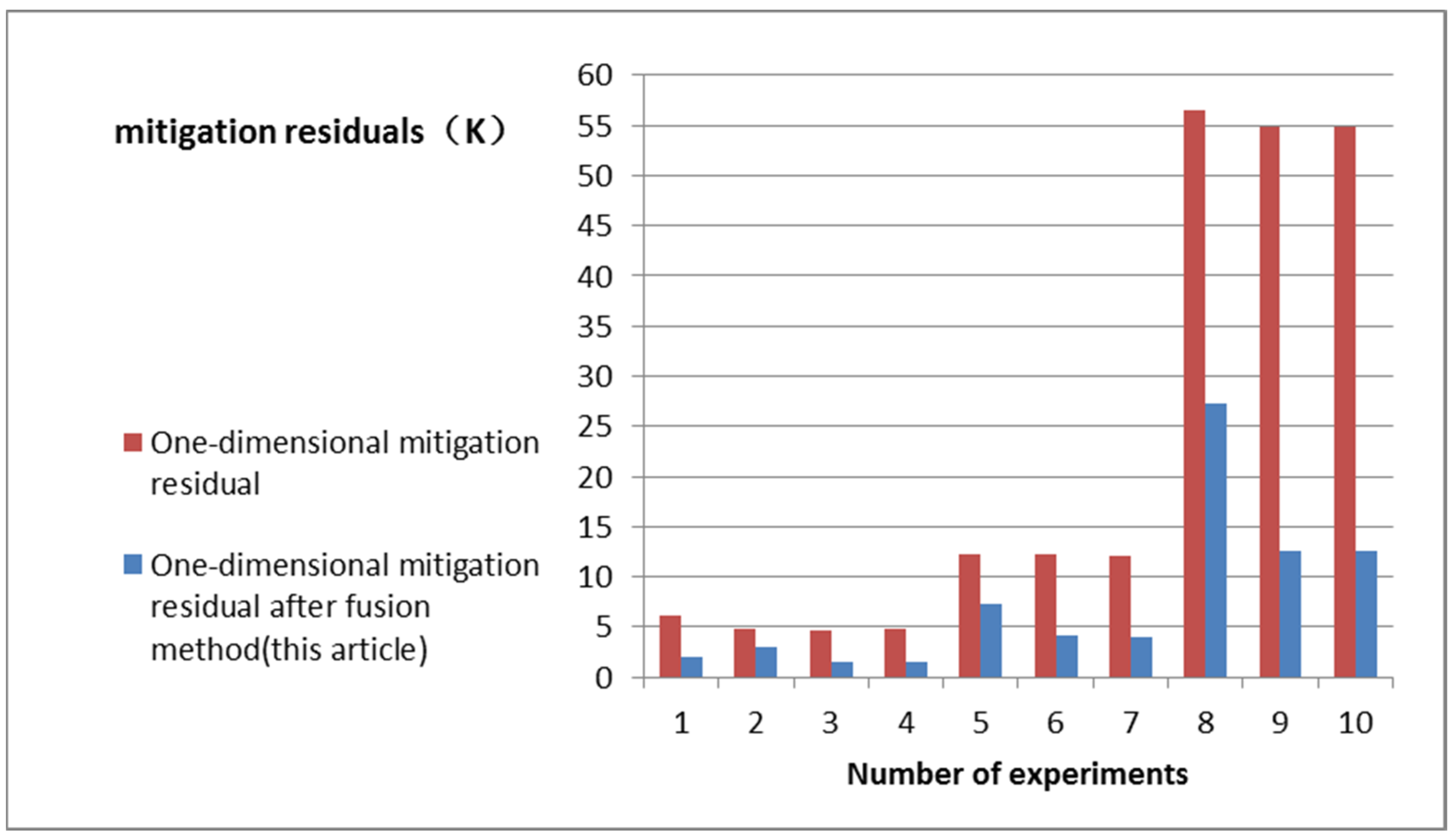
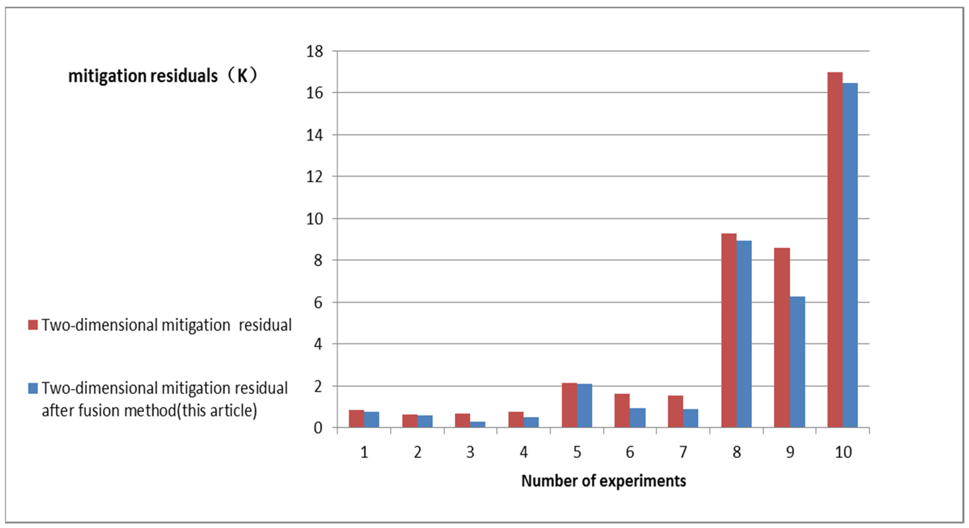
| Number | RFI-1 | RFI-2 | ξ | ξ-Error | η | η-Error | Intensity (K) | Intensity Error (K) | Residual Error (K) | Method |
|---|---|---|---|---|---|---|---|---|---|---|
| 1. | A | A | [0.1, −0.15] | 0 | [0, 0] | 0 | [450, 450] | 0 | 0 | True value |
| [0.0999, −0.1512] | [5.2528 × 10⁻⁵, 1.1749 × 10⁻³] | [0, 0] | 0 | [442.9808, 428.2634] | [7.0192, 21.7366] | 6.0813 | 1-D | |||
| [0.0996, −0.1498] | [3.6268 × 10⁻⁴, 2.2606 × 10⁻⁴] | [0, 5.0745 × 10⁻⁴] | [0, 5.0745 × 10⁻⁴] | [451.8538, 472.7692] | [1.8538, 22.7692] | 0.8460 | 2-D | |||
| [0.0999, −0.1499] | [3.7148 × 10⁻⁵, 5.5241 × 10⁻⁵] | [4.0596 × 10⁻⁵, 4.3133 × 10⁻⁴] | [4.0596 × 10⁻⁵, 4.3133 × 10⁻⁴] | [449.3511, 470.1507] | [0.6489, 20.1507] | [1.9754, 0.7648] | 1-D and 2-D fusion | |||
| 2. | A | B | [0.1, −0.15] | 0 | [0, 0] | 0 | [450, 1200] | 0 | 0 | True value |
| [0.1001, −0.1505] | [1.1439 × 10⁻⁴, 4.4619 × 10⁻⁴] | [0, 0] | 0 | [448.2988, 1.1846 × 10³] | [1.7012, 15.4470] | 4.7697 | 1-D | |||
| [0.0999, −0.1498] | [1.0896 × 10⁻⁴, 2.2606 × 10⁻⁴] | [0, −2.5372 × 10⁻⁴] | [0, 2.5372 × 10⁻⁴] | [451.6264, 1.2255 × 10³] | [1.6264, 25.5020] | 0.6152 | 2-D | |||
| [0.0999, −0.1503] | [6.5222 × 10⁻⁵, 3.1690 × 10⁻⁴] | [1.0149 × 10⁻⁵, 2.0298 × 10⁻⁵] | [1.0149 × 10⁻⁵, 2.0298 × 10⁻⁵] | [448.0629, 1.1996 × 10³] | [1.9371, 0.4432] | [2.9739, 0.5748] | 1-D and 2-D fusion | |||
| 3. | A | C | [0.1, −0.15] | 0 | [0, 0] | 0 | [450, 5500] | 0 | 0 | True value |
| [0.0999, −0.1500] | [6.8681 × 10⁻⁵, 9.0817 × 10⁻⁵] | [0, 0] | 0 | [447.0948, 5.4835 × 10³] | [2.9052, 16.5090] | 4.5906 | 1-D | |||
| [0.0996, −0.1500] | [3.6268 × 10⁻⁴, 2.7663 × 10⁻⁵] | [0, 0] | 0 | [454.0960, 5.5246 × 10³] | [4.0960, 24.6294] | 0.6842 | 2-D | |||
| [0.0999, −0.1500] | [1.1079 × 10⁻⁵, 2.7663 × 10⁻⁵] | [0, 2.5372 × 10⁻⁵] | [0, 2.5372 × 10⁻⁵] | [447.9541, 5.4984 × 10³] | [2.0458, 1.5607] | [1.4410, 0.2979] | 1-D and 2-D fusion | |||
| 4. | A | D | [0.1, −0.15] | 0 | [0, 0] | 0 | [450, 10,000] | 0 | 0 | True value |
| [0.1000, −0.1500] | [1.3880 × 10⁻⁵, 5.3126 × 10⁻⁵] | [0, 0] | 0 | [446.2804, 9.9833 × 10³] | [3.7196, 16.5090] | 4.8671 | 1-D | |||
| [0.1001, −0.1500] | [1.4477 × 10⁻⁴, 2.7663 × 10⁻⁵] | [0, 0] | 0 | [459.9269, 1.0026 × 10⁴] | [9.9269, 25.8676] | 0.7757 | 2-D | |||
| [0.0999, −0.1500] | [1.3698 × 10⁻⁵ 2.7663 × 10⁻⁵] | [0, 5.5819−5] | [0, 5.5819 × 10⁻⁵] | [447.9229, 9.9907 × 10³] | [2.0771, 9.2813] | [1.4410, 0.5119] | 1-D and 2-D fusion | |||
| 5. | B | B | [0.1, −0.15] | 0 | [0, 0] | 0 | [1200, 1200] | 0 | 0 | True value |
| [0.1009, −0.1500] | [8.8616 × 10⁻⁴, 7.6459 × 10⁻⁵] | [0, 0] | 0 | [1.1351 × 10³, 1.1947 × 10³] | [64.9144, 5.3119] | 12.1854 | 1-D | |||
| [0.0999, −0.1498] | [1.0896 × 10⁻⁴, 2.2606 × 10⁻⁴] | [−2.5372 × 10⁻⁴, 5.0745 × 10⁻⁴] | [2.5372 × 10⁻⁴, 5.0745 × 10⁻⁴] | [1.1979 × 10³, 1.2582 × 10³] | [2.0740, 58.1646] | 2.1379 | 2-D | |||
| [0.1002, −0.1500] | [1.0596 × 10⁻⁴, 1.8291 × 10⁻⁵] | [−3.5521 × 10⁻⁵, 5.0745 × 10⁻⁴] | [3.5521 × 10⁻⁵, 5.0745 × 10⁻⁴] | [1.1937 × 10³, 1.2492 × 10³] | [2.0740, 49.2069] | [7.3098, 2.0825] | 1-D and 2-D fusion | |||
| 6. | B | C | [0.1, −0.15] | 0 | [0, 0] | 0 | [1200, 5500] | 0 | 0 | True value |
| [0.1000, −0.1502] | [1.3880 × 10⁻⁵, 2.1645 × 10⁻⁴] | [0, 0] | 0 | [1.1894 × 10³, 5.4422 × 10³] | [10.6152, 57.8065] | 12.2051 | 1-D | |||
| [0.1001, −0.1500] | [1.4470 × 10⁻⁴, 2.7663 × 10⁻⁵] | [0, 0] | 0 | [1.2054 × 10³, 5.5647 × 10³] | [5.4376, 64.6948] | 1.6182 | 2-D | |||
| [0.1000, −0.1500] | [1.0375 × 10⁻⁵, 2.7663 × 10⁻⁵] | [−5.0745 × 10⁻⁴, 0] | [5.0745 × 10⁻⁴, 0] | [1.1945 × 10³, 5.4722 × 10³] | [5.5120, 27.8484] | [4.0999, 0.9106] | 1-D and 2-D fusion | |||
| 7. | B | D | [0.1, −0.15] | 0 | [0, 0] | 0 | [1200, 10,000] | 0 | 0 | True value |
| [0.1000, −0.1501] | [3.9964 × 10⁻⁵, 1.1415 × 10⁻⁴] | [0, 0] | 0 | [1.1935 × 10³, 9.9422 × 10³] | [6.4887, 57.7842] | 12.0188 | 1-D | |||
| [0.1001, −0.1500] | [1.4470 × 10⁻⁴, 2.7663 × 10⁻⁵] | [0, 0] | 0 | [1.1972 × 10³, 1.0060 × 10⁴] | [2.7948, 60.3195] | 1.5442 | 2-D | |||
| [0.1000, −0.1500] | [2.2944 × 10⁻⁵, 2.7663 × 10⁻⁵] | [0, −2.5372 × 10⁻⁵] | [0, 2.5372 × 10⁻⁵] | [1.1931 × 10³, 9.9762 × 10³] | [2.6948, 23.8132] | [4.0315, 0.8735] | 1-D and 2-D fusion | |||
| 8. | C | C | [0.1, −0.15] | 0 | [0, 0] | 0 | [5500, 5500] | 0 | 0 | True value |
| [0.1009, −0.1500] | [9.1128 × 10⁻⁴, 2.2615 × 10⁻⁵] | [0, 0] | 0 | [5.2013 × 10³, 5.4618 × 10³] | [298.7401, 38.2244] | 56.5578 | 1-D | |||
| [0.1001, −0.1500] | [1.4470 × 10⁻⁴, 2.7663 × 10⁻⁵] | [−2.5372 × 10⁻⁴, 5.0745 × 10⁻⁴] | [2.5372 × 10⁻⁴, 5.0745 × 10⁻⁴] | [5.4863 × 10³, 5.7588 × 10³] | [13.6773, 258.8316] | 9.2858 | 2-D | |||
| [0.1001, −0.1500] | [1.4470 × 10⁻⁴, 2.7663 × 10⁻⁵] | [−1.6238 × 10⁻⁵, 5.3790 × 10⁻⁴] | [1.6238 × 10⁻⁵, 5.3790 × 10⁻⁴] | [5.3872 × 10³, 5.6454 × 10³] | [13.6773, 145.3620] | [27.2677, 8.9380] | 1-D and 2-D fusion | |||
| 9. | C | D | [0.1, −0.15] | 0 | [0, 0] | 0 | [5500, 10,000] | 0 | 0 | True value |
| [0.0999, −0.1505] | [2.7401 × 10⁻⁵, 5.0901 × 10⁻⁴] | [0, 0] | 0 | [5.4576 × 10³, 9.7254 × 10³] | [42.3698, 274.5951] | 54.9054 | 1-D | |||
| [0.1001, −0.1500] | [1.4470 × 10⁻⁴, 2.7663 × 10⁻⁵] | [−2.5372 × 10⁻⁴, 2.5372 × 10⁻⁴] | [2.5372 × 10⁻⁴, 2.5372 × 10⁻⁴] | [5.4886 × 10³, 1.0247 × 10⁴] | [11.3719, 247.3988] | 8.5998 | 2-D | |||
| [0.1001, −0.1500] | [1.4470 × 10⁻⁴, 2.7663 × 10⁻⁵] | [−1.0656 × 10⁻⁴, 2.5372 × 10⁻⁴] | [1.0656 × 10⁻⁴, 2.5372 × 10⁻⁴] | [5.4826 × 10³, 1.0071 × 10⁴] | [11.3719, 71.2938] | [12.5556, 6.2873] | 1-D and 2-D fusion | |||
| 10. | D | D | [0.1, −0.15] | 0 | [0, 0] | 0 | [10,000, 10,000] | 0 | 0 | True value |
| [0.1009, −0.1500] | [9.1128 × 10⁻⁴, 7.8972 × 10⁻⁵] | [0, 0] | 0 | [9.4527 × 10³, 9.9336 × 10³] | [547.2665, 66.4243] | 54.9054 | 1-D | |||
| [0.1001, −0.1500] | [1.4470 × 10⁻⁴, 2.7663 × 10⁻⁵] | [−2.5372 × 10⁻⁴, 5.0745 × 10⁻⁴] | [2.5372 × 10⁻⁴, 5.0745 × 10⁻⁴] | [9.9769 × 10³, 1.0473 × 10⁴] | [23.1413, 472.8677] | 17.0032 | 2-D | |||
| [0.1001, −0.1500] | [1.4470 × 10⁻⁴, 2.7663 × 10⁻⁵] | [−2.3343 × 10⁻⁴, 5.5312 × 10⁻⁴] | [2.3343 × 10⁻⁴, 5.5312 × 10⁻⁴] | [9.7270 × 10³, 1.0159 × 10⁴] | [23.1413, 159.4105] | [12.5556, 16.4704] | 1-D and 2-D fusion |
Disclaimer/Publisher’s Note: The statements, opinions and data contained in all publications are solely those of the individual author(s) and contributor(s) and not of MDPI and/or the editor(s). MDPI and/or the editor(s) disclaim responsibility for any injury to people or property resulting from any ideas, methods, instructions or products referred to in the content. |
© 2024 by the authors. Licensee MDPI, Basel, Switzerland. This article is an open access article distributed under the terms and conditions of the Creative Commons Attribution (CC BY) license (https://creativecommons.org/licenses/by/4.0/).
Share and Cite
Zhang, L.; Jin, R.; Zhang, Q.; Wang, R.; Zhang, H.; Wen, Z. Fusion Method of RFI Detection, Localization, and Suppression by Combining One-Dimensional and Two-Dimensional Synthetic Aperture Radiometers. Remote Sens. 2024, 16, 667. https://doi.org/10.3390/rs16040667
Zhang L, Jin R, Zhang Q, Wang R, Zhang H, Wen Z. Fusion Method of RFI Detection, Localization, and Suppression by Combining One-Dimensional and Two-Dimensional Synthetic Aperture Radiometers. Remote Sensing. 2024; 16(4):667. https://doi.org/10.3390/rs16040667
Chicago/Turabian StyleZhang, Liqiang, Rong Jin, Qingjun Zhang, Rui Wang, Huan Zhang, and Zhongkai Wen. 2024. "Fusion Method of RFI Detection, Localization, and Suppression by Combining One-Dimensional and Two-Dimensional Synthetic Aperture Radiometers" Remote Sensing 16, no. 4: 667. https://doi.org/10.3390/rs16040667