A Robust Position Estimation Method in the Integrated Navigation System via Factor Graph

Abstract

Achieving higher accuracy and robustness stands as the central objective in the navigation field. In complex urban environments, the integrity of GNSS faces huge challenges and the performance of integrated navigation systems can be significantly affected. As the proportion of faulty measurements rises, it can result in both missed alarms and false positives. In this paper, a robust method based on factor graph is proposed to improve the performance of integrated navigation systems. We propose a detection method based on multi-conditional analysis to determine whether GNSS is anomalous or not. Moreover, the optimal weight of GNSS measurement is estimated under anomalous conditions to mitigate the impact of GNSS outliers. The proposed method is evaluated through real-world road tests, and the results show the positioning accuracy of the proposed method is improved by more than 60% and the missed alarm rate is reduced by 80% compared with the traditional algorithms.

1. Introduction

As the main source of global referenced positioning for Intelligent Transportation Systems (ITS), the Global Navigation and Positioning System (GNSS) can provide all-weather position information in outdoor scenarios [1]. Unfortunately, the positioning accuracy of GNSS is greatly affected by the environment. Interference, spoof, and outage occur frequently due to the multipath effects and non-line-of-sight (NLOS) receptions [2], which limit positioning accuracy. In contrast, the inertial navigation system (INS) can autonomously provide position information at a high output frequency with little dependence on the external environment but the navigation error will accumulate over time. GNSS/INS integrated navigation systems [3,4] make use of their advantages, which can provide high-precision and high-frequency navigation results. The popular existing GNSS/INS integration methods can be divided into filter frameworks and optimization frameworks.

Extended Kalman filter (EKF) based on filtering frameworks has been widely used to integrate different sensors due to its simple calculations and real-time performance [5]. However, from the mathematical interpretation, EKF can only iterate in a single step based on the first-order Markov assumption, which does not make full use of the historical information and is unable to perform correct repeated linearization. To solve this problem, unscented Kalman filter [6], and cubature Kalman filter [7] are proposed to improve the adaptability of nonlinear systems through more precise modeling. Furthermore, the iterated Kalman filter [8] is proposed to achieve multiple iterations, which significantly mitigates the linearization error. However, all these solutions did not fully utilize historical information. In addition, adding and removing sensors in filtering frameworks requires reconfiguration of the system, which increases complexity and time consumption.

The recently proposed factor graph optimization (FGO) [9] scheme provides a new view for multi-sensor fusion. Factor graphs have been widely used in Simultaneous Localization and Mapping (SLAM) to integrate diverse sensor measurements. In recent years, FGO has attracted much attention in the field of integrated navigation due to the advantages of multiple iterations, re-linearization, and the use of historical information [10]. The factor-graph-based multi-source fusion algorithms have been validated in simulations or experiments on several platforms, including aircraft, vehicles, and ships [11,12,13,14], which indicates that the FGO-based method is superior to the EKF-based method.

Although the potential of factor graph algorithms for positioning has been explored, it has also been shown that improved methods based on FGO are better adapted to the error distribution of multi-sensor fusion [15]. However, in complex environments, such as urban canyons, multipath, and NLOS, interference occurs frequently, which creates a greater impact on the accuracy of integrated navigation systems. A lot of research has been conducted on how to obtain more reliable and accurate GNSS positioning results, including detecting cycle slips by Melbourne-Wübbena [16] and geometry-free [17], which have significantly improved the data quality control. Nevertheless, there are still roughness and model-free errors in the observation that affect the localization accuracy.

Typically, methods to solve this problem can be classified into two categories: one is probabilistic statistics-based fault detection and isolation, which usually employ binary hypothesis tests based on residuals to detect faults then isolate them using the plug-and-play nature of the factor graph framework. The work described in [18] proposed a GNSS pseudorange fault detection method, which employs a chi-square test to detect faults and isolate them directly using factor graph. In [19], an iRAIM method is proposed where faults are detected in a fixed time window. The study in [20] combines the advantages of the sliding window and chi-square to allow faults to be estimated repeatedly to improve GNSS integrity. Similarly, the work in [21] uses the history information within a sliding window to fit new observations, reducing the effect of coarseness. However, all these solutions have a certain degree of time delay [22]. The other category is robust model-aided fault suppression. These strategies usually use a robust weight function to adjust the cost function to reduce the weight of the fault measurements, including the Huber kernel function [23], switchable constraints [24], dynamic covariance [25], etc. Wei et al. [26] proposed an improved factor graph fusion algorithm with enhanced robustness, which achieves the weight assignment and robust adjustment before the fusion of sensors, effectively reducing the adverse effect of sensor failures on the navigation results. Unfortunately, the weight function depends on the confidence distance and is restricted to [0, 1], which is not suitable for least squares approaches that require a continuous domain [27]. Yi et al. [28] proposed a robust loss function through parameter learning using a differentiable optimization. They use an end-to-end approach for learning state estimator modeled as the factor-graph-based smoother, which has a significant improvement over existing baselines. However, the use of neural networks for parameter estimation introduces a large computational effort. Nam et al. [29] built a robust adaptive state estimation framework based on the type-2 fuzzy inference system, which can learn the uncertainty by using particle swarm optimization, improving the robustness of the system. However, the increase in robustness usually implies a loss in accuracy; hence, the obtained solution is not optimal.

To overcome the limitations above, we propose an innovative IMU/GNSS/ODO loosely coupled integrated navigation framework based on factor graph. Firstly, inspired by the work in [30,31], to reduce the Inertial Measurement Unit (IMU) drift, an odometer (ODO) is derived to provide auxiliary measurements into the graph by constructing an IMU-ODO preintegration factor. Subsequently, we put forward a GNSS anomaly detection method based on multi-conditional analysis with a weighted fusion algorithm for adaptive covariance estimation. The original weighting estimate is used when the detection is normal and the adaptive covariance estimation is used for weighting when the test is anomalous, reducing the negative influence of faults. In addition, the impact of the delay in parameter estimation on the system accuracy is reduced by autonomously switching between the two weighting modes. The main contributions of the article are as follows:

• An IMU/GNSS/ODO integrated navigation framework based on factor graph is described. We accommodate the key parameters of each sensor and add ODO into preintegration to construct the IMU-ODO preintegration factor, which reduces the drift of IMU.
• To enhance the accuracy and robustness, an adaptive weighting estimation (AWE) algorithm is proposed, which can estimate the state and covariance simultaneously. We derive the principle of AWE from the maximum a posteriori (MAP) perspective.
• We put forward a GNSS anomaly detection method based on multi-conditional analysis. Through anomaly detection, the system achieves autonomous switching between two modes, original weighting estimation or adaptive weighting estimation, significantly reducing the missed alarm rate and time delays in fault recovery due to parameter estimation.

The remainder of this paper is organized as follows. Section 2 introduces the factor graph algorithm and the formulation in the IMU/GNSS/ODO integrated navigation system. Section 3 presents a robust factor graph optimization based on adaptive weighting estimation with multi-conditional analysis. The experiment results and discussion are presented to validate the effectiveness of the proposed algorithms in Section 4. Finally, the conclusion of this study is composed.

2. Factor Graph Algorithm and the Formulation in IMU/GNSS/ODO Integrated Navigation System

2.1. MAP Estimation and Factor Graph Algorithm

Factor graph is a bipartite undirected graphical model based on Bayesian networks [32], which encodes the links between variable nodes and measurements. The factor graph model solves the joint probability distribution of multivariate global functions based on the MAP estimation theory [33] to achieve information fusion.

The location issue can be described as an MAP problem:

$$\widehat{\mathit{X}}=\underset{\mathit{X}}{\arg \max }P(\mathit{X}\left|Z, u)\right.$$

(1)

where $\widehat{\mathit{X}}$ denotes the optimal estimation of the navigation-state variable and $\mathit{X}$ denotes the set of all navigation states. $Z$ represents all the measurements received by the system from the beginning. $u$ is the motion excitation or the output of the motion sensors and ${\mathit{u}}_k\in \mathit{u}$.

Since the inputs $u_k$ and measurements $z_k$ at each moment are independent of each other, according to Bayes’ law, the joint probability distribution function in Equation (1) can be factorized as:

$$\widehat{\mathit{X}}=\underset{\mathit{X}}{\arg \max }{\displaystyle \prod _{k}P(z_k|{\mathit{X}}_k)}{\displaystyle \prod _{k}P({\mathit{X}}_k|{\mathit{X}}_{k-1},{\mathit{u}}_k)}$$

(2)

where $z_k$ is the measurements at the time $t_k$. Equation (2) can be expressed as a product of individual factors. The optimal solution can be obtained by constructing and solving factor graphs.

A factor graph $G=(\mathit{F},\mathit{V},\mathit{\epsilon })$ [32,34] represents the joint probability distribution function of random variables where $\mathit{V}$ represents a set of variable nodes encoded by the navigation state, $\mathit{F}$ is a set of factor nodes, and $\mathit{\epsilon }$ represents a set of all edges connecting nodes. It consists of nodes and edges; nodes are divided into factor nodes $f_j\in \mathit{F}$ and variable nodes ${\mathit{X}}_k\in \mathit{V}$. The edges connecting the two nodes represent the error function ${\mathit{e}}_{k,j}(\cdot )\in \mathit{\epsilon }$, and each edge corresponds to a measurement $z_k$. The factor graph is defined as:

$$G(\mathit{X})={\displaystyle \prod _k{\mathit{f}}_k({\mathit{X}}_k)}$$

(3)

Assuming that the measurements are consistent with a Gaussian model [35]:

$${\mathit{f}}_k\left({\mathit{X}}_k\right)\propto \exp \left(-\frac{1}{2}{‖e({\mathit{X}}_k,z_k)‖}_{{\mathbf{\Sigma }}_k}^2\right)=\exp \left(-\frac{1}{2}{‖h_k\left({\mathit{X}}_k\right)-z_k‖}_{{\mathbf{\Sigma }}_k}^2\right)$$

(4)

where $e(\cdot )$ is the error function, which defines the error between the measurements $z_k$ and the observation $h_k(\cdot )$, ${‖e‖}_{{\mathbf{\Sigma }}_k}^2$ denotes the Mahalanobis distance, while ${\mathbf{\Sigma }}_k$ is the measurement noise covariance matrix, and $h_k(\cdot )$ denotes some known functions about state vectors. Based on Equations (3) and (4), the MAP estimation can be transformed into a nonlinear least squares problem:

$$\begin{array}{ll}\widehat{\mathit{X}}& =\underset{\mathit{X}}{\arg \min }{\displaystyle \sum _k{‖h_k\left({\mathit{X}}_k\right)-z_k‖}_{{\mathbf{\Sigma }}_k}^2}\\ & =\underset{\mathit{X}}{\arg \min }{\displaystyle \sum _{k}e}{\left({\mathit{X}}_k,z_k\right)}^{\mathrm{T}}{\mathbf{\Sigma }}_k{ }^{-1}e\left({\mathit{X}}_k,z_k\right)\\ & =\underset{\mathit{X}}{\arg \min }g({\mathit{X}}_k)\end{array}$$

(5)

Up until now, the inference of the factor graph is to find the optimal estimation $\widehat{\mathit{X}}$ by minimizing the objective function $g({\mathit{X}}_k)$ above.

The optimal estimation of $\widehat{\mathit{X}}$ can be solved by Gauss–Newton (G-N), Levenberg–Marquardt (L-M), dog-leg iteration [36], etc. To solve the least squares problem, we make the gradient of the objective function decrease by giving initial values and continuously updating the optimization variables through iterations, which transforms the problem of solving for a derivative of 0 into a problem of solving for a falling increment $\Delta \mathit{X}$. In addition, the incremental smoothing algorithm [14,37] is used to reduce the computational effort. Through the linearization process by nonlinear optimization methods, the corrected $\Delta \mathit{X}$ is obtained based on the initial estimate. According to L-M iteration, the increment $\Delta \mathit{X}$ meets the following equation [38]:

$$\Delta \widehat{\mathit{X}}=\arg \underset{\Delta \mathit{X}}{\min }{‖J{({\mathit{X}}_k)}^T\Delta \mathit{X}+e({\mathit{X}}_k,z_k)‖}^2, s.t.\parallel D\Delta \mathit{X}{\parallel }^2\le \rho$$

(6)

where $J({\mathit{X}}_k)$ represents the Jacobian matrix, $\mathit{D}$ donates the coefficient matrix and usually takes the unit matrix $I$, while $\rho$ is the radius of the trust domain.

Solving and updating $\Delta \mathit{X}$ requires upper triangular decomposition of $J({\mathit{X}}_k)$ by QR or Cholesky. Solving for (6) is equivalent to solving the incremental equation [34]:

$$(J^{T}J+\lambda I)\Delta {\mathit{X}}_k=-J\cdot e({\mathit{X}}_k,z_k)$$

(7)

where $\lambda$ is the Lagrange operator. The Jacobi matrix is equivalent to linearizing the factor graph, and its block structure determines the structure of the factor graph. The sparsity of the matrix is maintained by determining a specific order of variable elimination [39], and each update will only compute a small portion of the topology that has changed, effectively improving the real-time performance of the algorithm.

2.2. Factor Graph Formulation in Integrated Navigation System

From the principle of the factor graph, it can be noted that the selection of system-state variables and the establishment of error functions are the main factors affecting the performance of the algorithm. Considering the key parameters of each sensor and adding ODO into preintegration, the factor formulation for measurement models is deduced.

A.

Formulation

During the navigation process, the parameters of each sensor change over time [40]. Accuracy can be improved by expanding the dimension of the state variables and adding the key parameters into the optimized estimation. Considering the ODO scale factor error, the state variables of the integrated INS/GNSS/ODO navigation system are selected as:

$$\mathit{X}(k)=[\begin{array}{llllll}{({\mathit{p}}_{w{b}_k}^w)}^T\hfill & {(v_{w{b}_k}^w)}^T\hfill & {(q_{w{b}_k}^w)}^T\hfill & {({\mathit{\epsilon }}_{{\mathrm{g}}_k})}^T\hfill & ({\mathit{\nabla }}_{a_k}{)}^T& c_k]\end{array}$$

(8)

where the state $\mathit{X}(k)$ includes the position ${\mathit{p}}_{w{b}_k}^w$, velocity ${\mathit{v}}_{w{b}_k}^w$, and attitude ${\mathit{q}}_{w{b}_k}^w$ in the world frame (w-frame), along with the gyroscope biases ${\mathit{\epsilon }}_{{\mathrm{g}}_k}$, accelerometer biases ${\mathbf{\nabla }}_{a_k}$, and ODO scale factor $c_k$. $b_k$ is the body frame (b-frame) at $k$.

B.

IMU-ODO Preintegration Factor

Odometer information is typically used as the forward speed to provide an aid; however, in reality, the raw measurement information of an odometer is the mileage, and obtaining an accurate auxiliary speed relies on accurate motion modeling. The preintegration method is utilized to convert the odometer mileage into displacement, forming the IMU-ODO preintegration model instead of the traditional IMU preintegration model.

The MEMS-INS mechanization [41] can be expressed as:

$$\begin{array}{l}{v}_{w{b}_k}^w=v_{w{b}_{k-1}}^w+C_{b_{\mathrm{k}-1}}^w{v}_{b_{k-1}}^{b_k}+g^w\Delta t_k\\ p_{w{b}_k}^w=p_{w{b}_{k-1}}^w+v_{w{b}_{k-1}}^w\Delta t_k+\frac{1}{2}{g}^w\Delta t_k^2+\frac{1}{2}{C}_{b_{k-1}}^w{v}_{b_{k-1}}^{b_k}\Delta t_k\\ q_{w{b}_k}^w=q_{w{b}_{k-1}}^w\otimes q_{b_{k-1}}^{b_k}\end{array}$$

(9)

where ${\mathit{C}}_{b_{\mathrm{k}-1}}^w$ denotes the rotation matrix from the b-frame to the w-frame; ${\mathit{g}}^w$ is the gravity in the w-frame; ${\mathit{v}}_{w{b}_{k-1}}^w$ and ${\mathit{p}}_{w{b}_{k-1}}^w$ are the velocity and position of the b-frame relative to the w-frame projected on the w-frame; ${\mathit{q}}_{w{b}_k}^w$ is the quaternion; and ${\mathit{q}}_{b_{k-1}}^{b_k}$ and ${\mathit{v}}_{b_{k-1}}^{b_k}$ are the increments of attitude and velocity from the $k-1$ to the $k$, respectively:

$$\begin{array}{l}{v}_{b_{k-1}}^{b_k}\approx \Delta v_{\mathit{f},k}^b+\frac{1}{2}\Delta {\theta }_k\times \Delta v_{\mathit{f},k}^b\\ q_{b_{k-1}}^{b_k}\approx \left[\begin{array}{c}\cos ‖\frac{1}{2}\Delta {\theta }_k‖\\ \frac{\sin ‖\frac{1}{2}\Delta {\theta }_k‖}{‖\Delta {\theta }_k‖}\Delta {\theta }_k\end{array}\right]\\ \Delta v_{\mathit{f},k}^b={\displaystyle {\int }_{t_{k-1}}^{t_k}({\mathit{f}}^b-{\nabla }_{a_k}-{\mathit{n}}_a)}dk\\ \Delta {\theta }_k={\displaystyle {\int }_{t_{k-1}}^{t_k}\left[{\omega }^b-{\mathit{\epsilon }}_{g_k}-{\mathit{n}}_g\right]}dk\end{array}$$

(10)

where ${\mathit{f}}^b$ and ${\mathit{\omega }}^b$ are the specific force and angular rate in the b-frame. $\Delta v_{\mathit{f},k}^b$ and $\Delta {\theta }_k$ are the velocity and angle of the integration of accelerometer and gyroscope outputs. ${\mathit{n}}_a$ and ${\mathit{n}}_g$ represent the gyroscope and accelerometer white noise, respectively.

When ODO observations are introduced, considering the nonholonomic constraints, the velocity from the b-frame to the vehicle co-ordinate (v-frame) can be expressed as follows [30]:

$$v_{w{v}_k}^w=v_{w{b}_k}^w+C_{b_k}^w\left[{\omega }_{w{b}_k}^{b_k}\times \right]I_{odo}^b$$

(11)

where ${\mathit{I}}_{odo}^b$ donates the lever arm for the odometer.

The mileage increment derived from velocity is:

$$s_{b_{k-1}}^{b_k}\approx C_v^b{s}_{v_{k-1}}^{v_k}-C_{b_{k-1}}^{b_k}{I}_{\mathrm{odo} }^b+I_{\mathrm{odo} }^b$$

(12)

where ${\mathit{C}}_v^b$ is the mounting angle of the IMU, ${\mathit{s}}_{v_{k-1}}^{v_k}$ is the increment of ODO, denoted as ${\mathit{s}}_{v_{k-1}}^{v_k}=s^v(1+c_k)$ and ${\mathit{s}}^v$ represents the output of the ODO, and $C_{b_{k-1}}^{b_k}$ is the direction cosine matrix of ${\mathit{q}}_{b_{k-1}}^{b_k}$.

Therefore, the position can be updated by the IMU and ODO, represented as:

$$p_{w{b}_k}^w=p_{w{b}_{k-1}}^w+C_{b_{k-1}}^w[C_v^b{s}_{v_{k-1}}^{v_k}+(1-C_{b_{k-1}}^{b_k})I_{\mathrm{odo} }^b]$$

(13)

According to (9) and (13), the IMU-ODO preintegration factor is constructed as:

$${\mathit{f}}^{IMU-ODO}\left({\mathit{X}}_{k+1},{\mathit{X}}_k,{\mathit{\epsilon }}_{g_k},{\nabla }_{a_k},c_k\right)\triangleq d\left({\mathit{X}}_{k+1}-h_k^{INS}\left({\mathit{X}}_k,{\mathit{\epsilon }}_{g_k},{\nabla }_{a_k},c_k,z_k\right)\right)$$

(14)

The equivalent IMU factor [9] updates in the b-frame, which leads to large errors when the motion changes rapidly. Therefore, the classical INS mechanization [42,43] is used for updating during the preintegration period, ${\mathit{X}}_{\mathit{k}}^{\mathit{I}\mathit{N}\mathit{S}-\mathit{O}\mathit{D}\mathit{O}}$ is the estimated value of the navigation state variable obtained from the IMU-ODO mechanization, and INS-ODO factor node is:

$${\mathit{f}}^{\mathit{I}\mathit{N}\mathit{S}-\mathit{O}\mathit{D}\mathit{O}}\left({\mathit{X}}_k\right)\triangleq d\left({\mathit{X}}_k-{\mathit{X}}_k^{INS-ODO}\right)$$

(15)

Suppose that the bias ${\mathit{k}}_k=({\mathit{\epsilon }}_{g_k},{\nabla }_{a_k},c_k)$, the bias node can be expressed as:

$${\mathit{f}}^{bias}(k_k,k_{k-1})\triangleq d(k_k-u(k_k))$$

(16)

where $u({\mathit{k}}_k)$ is the stochastic wandering model with bias parameters.

Since the bias of the inertial navigation system does not change significantly in a short period, it can be inserted into the factor graph model at a lower frequency, which can reduce the amount of computation without loss of accuracy.

C.

GNSS Positioning Factor

The GNSS positioning results and covariance ${\mathbf{\Sigma }}_i^{GNSS}$ can be obtained from the GNSS receiver. Hence, the measurement equation considering the lever-arm effect can be expressed as:

$${\mathit{p}}_{\mathit{G}\mathit{N}\mathit{S}\mathit{S},k}^w={\mathit{p}}_{w{b}_k}^w+{\mathit{R}}_{b_k}^w{\mathit{l}}^b+n_k^{GNSS}$$

(17)

where ${\mathit{p}}_{\mathit{G}\mathit{N}\mathit{S}\mathit{S},k}^w$ is the GNSS position in the w-frame, ${\mathit{n}}_k^{\mathit{G}\mathit{N}\mathit{S}\mathit{S}}$ is the measurement position noise, and ${\mathit{l}}^b$ denotes the lever-arm error of GNSS antenna. ${\mathit{R}}_{b_k}^w$ is the rotation matrix from the b-frame to the w-frame. Then, the GNSS factor node can be expressed as:

$${\mathit{f}}^{GNSS}(p_{w{b}_k}^w)\triangleq d\left(p_{w{b}_k}^w+R_{b_k}^w{l}^b-p_{GNSS,k}^w\right)$$

(18)

D.

IMU-ODO/GNSS factor graph model

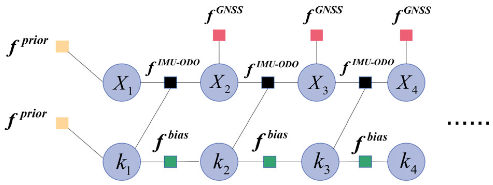
In summary, we derive the IMU-ODO preintegration model and the GNSS measurement model to form the IMU-ODO/GNSS integrated navigation system. When the GNSS measurement information arrives, the corresponding factor node is connected to the INS node constructed by IMU-ODO. The factor graph model of the whole navigation system is shown in Figure 1.

We minimize the sum of the prior and Mahalanobis distances for all residuals to obtain the MAP estimate:

$$\underset{\mathit{X}}{{\displaystyle \min }}\left\{\begin{array}{c}{‖r_0-h_0\mathit{X}‖}^2+{\displaystyle \sum _{k\in [1,n]}{‖r_{IMU-ODO}\left(z_{k-1,k}^{IMU-ODO },\mathit{X}\right)‖}_{{\mathbf{\Sigma }}_{k-1,k}^{IMU-ODO}}^2}\\ +{\displaystyle \sum _{i\in [0,m]}{‖r_{GNSS}\left(z_i^{GNSS},\mathit{X}\right)‖}_{{\mathbf{\Sigma }}_i^{GNSS}}^2}\end{array}\right\}$$

(19)

where $\{{\mathit{r}}_0,{\mathit{h}}_0\}$ represents the priori information and ${\mathit{r}}_{\mathit{I}\mathit{M}\mathit{U}-\mathit{O}\mathit{D}\mathit{O}}$ and ${\mathit{r}}_{GNSS}$ are the residual of the IMU-ODO preintegrating factors and GNSS factors, respectively. $m,n$ are the number of GNSS and IMU-ODO preintegrating factors, respectively. Ceres solver is used to solve this problem.

3. Robust Factor Graph Optimization Based on Adaptive Weighting Estimation with Multi-Conditional Analysis

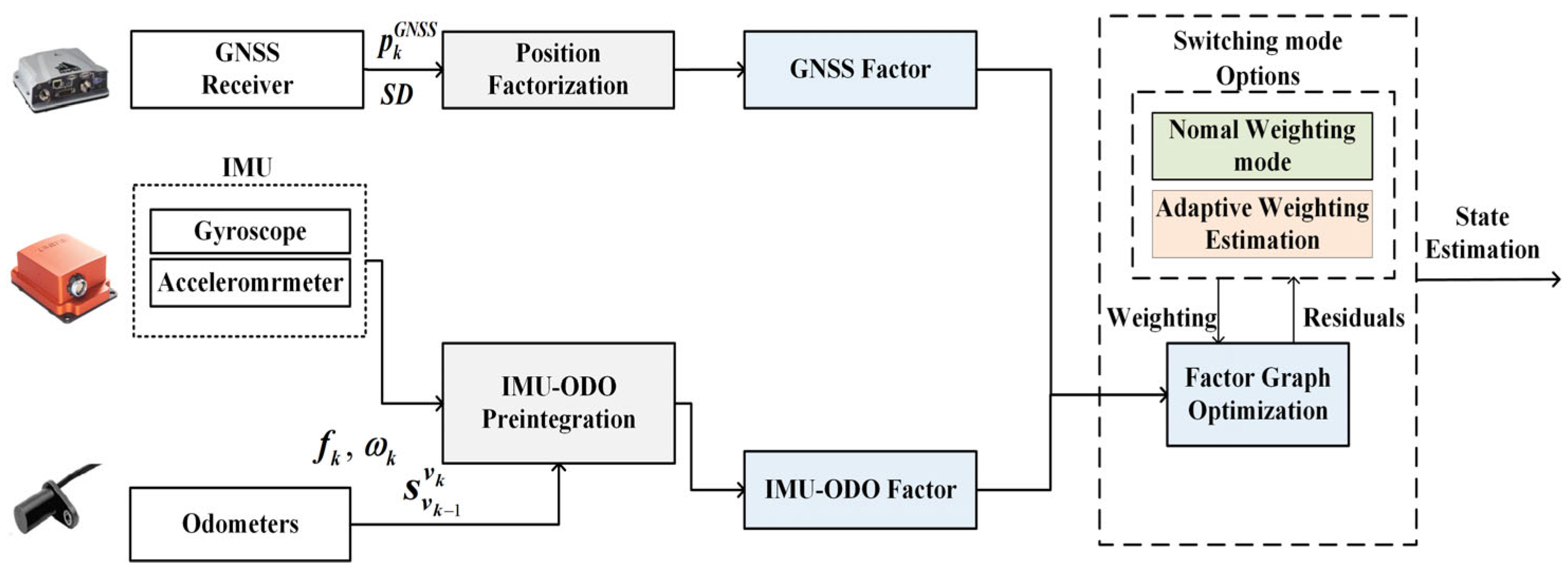
In this section, we will introduce a novel GNSS anomaly detection method and an adaptive covariance estimation algorithm to enhance accuracy and robustness. An overview of the method proposed is shown in Figure 2. The FGO integrates multi-sensor measurements aided by the weighting from the switching mode options. The whole process is called switching adaptive weighting estimation factor graph optimization (SAWE-FGO) in this paper.

3.1. GNSS Anomaly Detection Based on Multi-Conditional Analysis

Based on Equation (17), the residual of the GNSS factor can be obtained as follows:

$$r_{GNSS}\left(z_k^{GNSS},\mathit{X}\right)=p_{{\mathrm{wb}}_k}^{\mathrm{w}}+R_{{\mathrm{b}}_k}^{\mathrm{w}}{l}^b-p_{GNSS,k}^{\mathrm{w}}$$

(20)

Assuming that the observation model and the IMU-ODO model do not contain errors, this yields the following conditional density on the measurement $z_k$:

$$P(z_k|{\mathit{X}}_k)=\mathcal{N}(z_k;h_k({\mathit{X}}_k),{\mathbf{\Sigma }}_0)=\frac{1}{{(2\pi )}^{k/2}\sqrt{\left|{\mathbf{\Sigma }}_0\right|}}\exp \left\{-\frac{1}{2}\Vert h_k^{GNSS}({\mathit{X}}_k)-z_k{\Vert }_{{\mathbf{\Sigma }}_0}^2\right\}$$

(21)

If the GNSS equipment fails, the statistical nature of the measurement noise changes and the mean of the residual ${\mathit{r}}_{\mathit{G}\mathit{N}\mathit{S}\mathit{S}}(k)$ will no longer be equal to 0, as described below.

According to the binary hypothesis to ${\mathit{r}}_{\mathit{G}\mathit{N}\mathit{S}\mathit{S}}(k)$, $H_0$ indicates that there are no faults:

$$E\{{\mathit{r}}_{\mathit{G}\mathit{N}\mathit{S}\mathit{S}}(k)\}=0,\hspace{1em}E\{{\mathit{r}}_{\mathit{G}\mathit{N}\mathit{S}\mathit{S}}(k){\mathit{r}}_{\mathit{G}\mathit{N}\mathit{S}\mathit{S}}{(k)}^T\}={\mathbf{\Sigma }}_0$$

(22)

$H_1$ indicates a malfunction:

$$E\{{\mathit{r}}_{\mathit{G}\mathit{N}\mathit{S}\mathit{S}}(k)\}=\mu ,\hspace{1em}E\{({\mathit{r}}_{\mathit{G}\mathit{N}\mathit{S}\mathit{S}}(k)-\mu ){({\mathit{r}}_{\mathit{G}\mathit{N}\mathit{S}\mathit{S}}(k)-\mu )}^T\}={\mathbf{\Sigma }}_0$$

(23)

Since the residuals have three dimensions, latitude, longitude, and height, the same judgment criterion can be used in each dimension. The residual criterion in one dimension is as follows:

$$\left\{\begin{array}{c}i\mathit{f} r_{\mathit{G}\mathit{N}\mathit{S}\mathit{S}}(k)>r_1, \mathrm{fault}\\ i\mathit{f} r_{\mathit{G}\mathit{N}\mathit{S}\mathit{S}}(k)\le r_1, \mathrm{nomal}\end{array}\right.$$

(24)

where $r_1$ is the threshold for the judgment. ${\mathit{r}}_{\mathit{G}\mathit{N}\mathit{S}\mathit{S}}(k)$ represents the residual between the measured value and the predicted value; thus, the larger ${\mathit{r}}_{\mathit{G}\mathit{N}\mathit{S}\mathit{S}}(k)$ is, the less reliable the measurement information is. The selection of $r_1$ will affect the results of fault detection. If $r_1$ is too large, it will lead to a high rate of missed alarms. Inversely, if $r_1$ is too small, it will not be able to meet the statistical characteristics. The threshold value can be set according to the accuracy and performance of different sensors, but the basic criterion is to set it between the maximum probability value of the independent variable and the mean of the chi-square distribution. In this paper, we have chosen the value of $r_1$ to be 0.2.

Using the Mahalanobis distance of residuals, the chi-square test is simple in operation and small in computation compared to sequential methods with the same number of samples. However, this approach introduces missed alarms and time delays for slow-change faults. Therefore, the GNSS and IMU-ODO preintegrated incremental error criterion is provided to assist the residuals in determining whether there is an anomaly in the standard deviations (SD) of latitude, longitude, and altitude measurement.

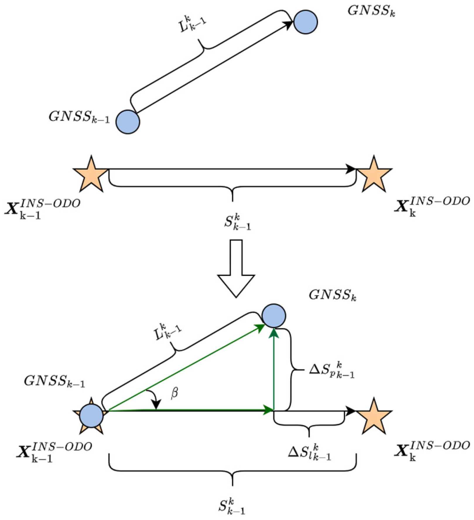
During a GNSS epoch, the IMU-ODO preintegration is recursed in increments, with mileage increments ${\mathit{S}}_{k-1}^k$. Obtained from the IMU-ODO mechanization, ${\mathit{X}}_{\mathrm{k}-1}^{\mathit{I}\mathit{N}\mathit{S}-\mathit{O}\mathit{D}\mathit{O}}$ and ${\mathit{X}}_{\mathrm{k}}^{\mathit{I}\mathit{N}\mathit{S}-\mathit{O}\mathit{D}\mathit{O}}$ are the navigation-state estimates for two neighboring moments without the GNSS fusion. ${\mathit{L}}_{\mathit{k}-1}^{\mathit{k}}$ represents displacement increments from the GNSS result of the previous epoch. Since relative changes are described, to accurately reflect the incremental changes, we align $\mathit{G}\mathit{N}\mathit{S}{\mathit{S}}_{k-1}$ with ${\mathit{X}}_{\mathrm{k}-1}^{\mathit{I}\mathit{N}\mathit{S}-\mathit{O}\mathit{D}\mathit{O}}$ in position and use vector decomposition in the b-frame, as shown in Figure 3.

The longitudinal and lateral incremental error can be expressed as:

$$\begin{array}{l}\Delta {\mathit{S}}_{lk-1}^k={\mathit{S}}_{k-1}^k-{\mathit{L}}_{k-1}^k\cos \beta \\ \Delta {\mathit{S}}_{pk-1}^k={\mathit{L}}_{k-1}^k\sin \beta \end{array}$$

(25)

Thus, the incremental error of IMU-ODO preintegration with GNSS is:

$$\Delta S_{k-1}^k=\sqrt{{(\Delta {\mathit{S}}_p{ }_{k-1}^k)}^2+{(\Delta {\mathit{S}}_l{ }_{k-1}^k)}^2}$$

(26)

The incremental error criterion is:

$$\left\{\begin{array}{c}if \Delta S_{k-1}^k>s_1, \mathrm{fault}\\ if \Delta S_{k-1}^k\le s_1, \mathrm{nomal}\end{array}\right.$$

(27)

Under normal GNSS operation, the displacement increments of GNSS and the mileage increment of IMU-ODO are in the same trend for a short period and the incremental error between them is very small. When the GNSS is abnormal, the GNSS increment will be much larger than the IMU-ODO mileage increment, which generates a large incremental error. The threshold $s_1$ is set to the maximum possible probability value of the independent variable; here, we choose 0.45.

The detection method combines residual judgment, SD judgment, GNSS, and IMU-ODO incremental error judgment. It is specifically divided into four categories as

Table 1. Combined failure diagnosis rule.

Case No.	Residual	SD	Incremental Error	Diagnosis Result	Mode Judgment Result
1	T	T	/	T	T
2	F	F	/	F	T
3	T	F	/	F	F
4	F	T	F	F	F
			T	T	T

shown.

In cases 1 or 2, the result is judged to be a normal condition when residual and SD methods detect it identically. In case 3, the combination of judgments has a lower probability because false positives are small probability events in navigation systems. In case 4, which is a priority for us, the SD shows GNSS signals are normal at this moment, while the residual method displays exceptions, known as missed alarms of SD. The original SD values become implausible under this condition. Thus, using the original SD values as covariates will increase the percentage of fault measurement in integrated navigation systems. Since the residual is more sensitive to faults, extra time is required for the system to return to normal as faults accumulate. We introduce the incremental displacement errors of GNSS and IMU-ODO preintegration to assist in determining the end of the failure event. If the incremental error determines that the system has returned to normal, we choose to use the original SD from then on.

Therefore, the switchable GNSS factor error function can be written as:

$$\parallel {\mathit{e}}_i^{GNSS}{\parallel }^2=\left\{\begin{array}{c} {(z_i-h^{GNSS}(X_i))}^T{\Sigma }_0(z_i-h^{GNSS}(X_i)), \mathrm{mode} \mathrm{judgment} \mathrm{result}=\mathrm{T} \\ {(z_i-h^{GNSS}(X_i))}^T{\Sigma }_i(z_i-h^{GNSS}(X_i)), \mathrm{mode} \mathrm{judgment} \mathrm{result}=\mathrm{F}\end{array}\right.$$

(28)

When the results are judged normal, it means that the edges associated with the variables are added to the graph entirely and the GNSS covariance is computed using the original SD; when the results are judged abnormal, the proportion of the edges added to the graph is decided by the weight obtained from adaptive covariance estimation. The optimization can be defined on R instead of [0, 1] in existing methods.

3.2. Adaptive Weighting Estimation

If the results are judged to be abnormal, the GNSS SD at this time can no longer correctly reflect the degree of data correlation. Therefore, when the result is abnormal, the factor graph optimization becomes both a state and covariance estimation problem. Then, the cost function becomes:

$$J(\mathit{X},\mathbf{\Sigma })=\frac{1}{2}{\displaystyle \sum _{i=1}^k\mathit{e}{\left(X_i,z_i\right)}^{\mathrm{T}}{\mathbf{\Sigma }}_i{ }^{-1}\mathit{e}\left(X_i,z_i\right)}$$

(29)

where $\mathbf{\Sigma }=\{{\Sigma }_1,{\Sigma }_2\cdots {\Sigma }_k\}$ is the unknown covariance matrix.

The MAP problem can be modified to:

$$\{\widehat{\mathit{X}},\widehat{\mathbf{\Sigma }}\}=\arg \underset{\{\mathit{X},\mathbf{\Sigma }\}}{\min }J(\mathit{X},\mathbf{\Sigma })=\arg \underset{\{\mathit{X},\mathbf{\Sigma }\}}{\min }\{-\ln P(\mathit{X},\mathbf{\Sigma }|z)\}$$

(30)

where $\widehat{\mathbf{\Sigma }}$ is the estimate of the covariance matrix.

The decomposition of the posterior probability can be obtained:

$$P(\mathit{X},\mathbf{\Sigma }|z)=P(\mathit{X}|z,\mathbf{\Sigma })P(\mathbf{\Sigma })={\displaystyle \prod _{i=1}^{k}P({\mathit{X}}_i|z_i,{\mathbf{\Sigma }}_i)P({\mathbf{\Sigma }}_i)}$$

(31)

According to Bayes’ rule, decomposing the posterior probability density $P({\mathit{X}}_i|z_i,{\mathbf{\Sigma }}_i)$ is obtained:

$$P({\mathit{X}}_i|z_i,{\mathbf{\Sigma }}_i)=\frac{P(z_i|{\mathit{X}}_i,{\mathbf{\Sigma }}_i)P({\mathit{X}}_i)}{P(z_i)}\propto P(z_i|{\mathit{X}}_i,{\mathbf{\Sigma }}_i)P({\mathit{X}}_i)$$

(32)

where $P({\mathit{X}}_i)$ and $P(z_i)$ are the a priori probability densities for prediction ${\mathit{X}}_i$ and measurement $z_i$, respectively. $P(z_i)$ has nothing to do with ${\mathit{X}}_i$ and $z_i$, so it can be ignored. Since there is no priori covariance, the conditional probability density $p(z_i|X_i,{\Sigma }_i)$ is denoted [44]:

$$P(z_i|{\mathit{X}}_i,{\mathbf{\Sigma }}_i)=\frac{1}{\sqrt{{(2\pi )}^k\det ({\mathbf{\Sigma }}_i)}}\exp \left\{-\frac{1}{2}e{({\mathit{X}}_i,z_i)}^{\mathrm{T}}{\mathbf{\Sigma }}_i{ }^{-1}\mathit{e}({\mathit{X}}_i,z_i)\right\}$$

(33)

where $\det ({\mathbf{\Sigma }}_i)$ is the determinant of the matrix ${\mathbf{\Sigma }}_i$. However, if there is no a priori knowledge of the ${\mathbf{\Sigma }}_i$, an accurate estimate of the state ${\mathit{X}}_i$ is not available in practice. Then, we obtain only an approximation of the state ${\widehat{\mathit{X}}}_i$ and the likelihood probability density will change to:

$$P(z_i|{\mathit{X}}_i,{\mathbf{\Sigma }}_i)=\frac{1}{\sqrt{{(2\pi )}^k\det ({\mathit{R}}_i)}}\exp \left\{-\frac{1}{2}e{({\widehat{\mathit{X}}}_i,z_i)}^{\mathrm{T}}{\mathit{R}}_i^{-1}\mathit{e}({\widehat{\mathit{X}}}_i,z_i)\right\}$$

(34)

Combining Equations (30), (32), and (34), the objective function can be written as:

$$J(\mathit{X},\mathbf{\Sigma })\propto \frac{1}{2}{\displaystyle \sum _{i=1}^k[\mathit{e}{({\widehat{\mathit{X}}}_i,z_i)}^{\mathrm{T}}{\mathit{R}}_i^{-1}\mathit{e}({\widehat{\mathit{X}}}_i,z_i)-\ln (\det ({\mathit{R}}_i^{-1}))-k\ln (2\pi )]}$$

(35)

where ${\mathit{R}}_i$ denotes the residual covariance matrix after the $i$ observation. Our strategy is to find the optimal ${\mathbf{\Sigma }}_i$ to eliminate it from the expression. Assuming that the covariance matrices of the same observations are the same. The derivation of Equation (35) with respect to ${\mathit{R}}_i^{-1}$ and letting the derivative be 0 yields $R_i$:

$${\mathit{R}}_i=\frac{1}{k}{\displaystyle \sum _{i=1}^k\mathit{e}({\widehat{\mathit{X}}}_i,z_i)\mathit{e}{({\widehat{\mathit{X}}}_i,z_i)}^T}$$

(36)

The residual sequence can be approximated as:

$$\mathit{e}({\widehat{\mathit{X}}}_i)=z_i-h({\widehat{\mathit{X}}}_i)\approx z_i-{\mathit{\varphi }}_i{\widehat{\mathit{X}}}_i=z_i-{\mathit{\varphi }}_i({\mathit{X}}_i+\delta {\widehat{\mathit{X}}}_i)={\mathit{n}}_i-{\mathit{\varphi }}_i\delta {\widehat{\mathit{X}}}_i$$

(37)

where ${\mathit{\varphi }}_i$ is the Jacobian of the measurement function and $\delta {\widehat{\mathit{X}}}_i$ is the estimation error of the navigation state. ${\mathit{n}}_i$ is the measurement noise.

The propagation process of the covariance is derived below:

$$\begin{array}{l}{R}_i=\mathrm{E}(e_i({\widehat{\mathit{X}}}_i)e_i{({\widehat{\mathit{X}}}_i)}^T)\\ =E[(n_i-{\mathit{\varphi }}_i\delta {\widehat{\mathit{X}}}_i){(n_i-{\mathit{\varphi }}_i\delta {\widehat{\mathit{X}}}_i)}^T]\\ =E(n_i{n}_i{ }^T)+{\mathit{\varphi }}_{i}E(\delta {\widehat{\mathit{X}}}_i\delta {\widehat{\mathit{X}}}_i{ }^T){\mathit{\varphi }}_i{ }^T-E(\mathit{\varphi }\delta {\widehat{\mathit{X}}}_i)\underset{0}{\underbrace{E(n_i{ }^T)}}-\underset{0}{\underbrace{E(n_i)}}E(\delta {\widehat{\mathit{X}}}_i{ }^T{\mathit{\varphi }}^T)\\ =E(n_i{n}_i{ }^T)+{\mathit{\varphi }}_{i}E(\delta {\widehat{\mathit{X}}}_i\delta {\widehat{\mathit{X}}}_i{ }^T){\mathit{\varphi }}_i{ }^T\\ ={\mathbf{\Sigma }}_i+{\mathit{\varphi }}_i{Q}_{{\widehat{\mathit{X}}}_i|z_i}{\mathit{\varphi }}_i{ }^T\end{array}$$

(38)

where ${\mathit{Q}}_{{\widehat{\mathit{X}}}_i|z_i}$ is a posteriori covariance matrix updated with the IMU preintegrated error model:

$$Q_{{\widehat{\mathit{X}}}_{i+1}|z_i}=Q_{{\mathit{X}}_{i+1,i}}-Q_{{\mathit{X}}_{i+1},z_i}{\mathit{\Sigma }}_i{ }^{-1}{Q}_{z_i,{\mathit{X}}_{i+1}}$$

(39)

$$\left\{\begin{array}{l}{Q}_{{\mathit{X}}_{i+1,i}}=M_i{Q}_{{\mathit{X}}_i}{M}_i^{\mathrm{T}}+N_i{\mathit{\Sigma }}^a{N}_i^{\mathrm{T}}+{\mathit{F}}_i{\mathit{\Sigma }}^{\mathrm{g}}{\mathit{F}}_i^{\mathrm{T}}\hfill \\ Q_{{\mathit{X}}_{i+1},z_i}=Q_{{\mathit{X}}_{i+1,i}}{H}_i^{\mathrm{T}}\hfill \\ Q_{z_i,{\mathit{X}}_{i+1}}=H_k{Q}_{{\mathit{X}}_{i+1,i}}\hfill \end{array}\right.$$

(40)

where $M_i$ is the derivation of Equation (9) with respect to position, velocity, and attitude. $N_i$ and ${\mathit{F}}_i$ are the derivations of the equations of motion with respect to force and angular velocity. ${\Sigma }_{ }^a$ and ${\Sigma }_{ }^{\mathrm{g}}$ are the measurement noise of the accelerometer and gyroscope, respectively.

Thus, the estimation of the measurement covariance can be obtained:

$${\mathbf{\Sigma }}_i={\mathit{R}}_i-{\mathit{\varphi }}_i{\mathit{Q}}_{{\widehat{X}}_i|z_i}{\mathit{\varphi }}_i^T$$

(41)

From the derivation, it can be seen that the estimation ${\mathbf{\Sigma }}_i$ requires a priori ${\mathit{R}}_i$, where the a priori value is averaged over the residual covariance of all observations before switching to adaptive weight estimation.

4. Experiment Results and Discussion

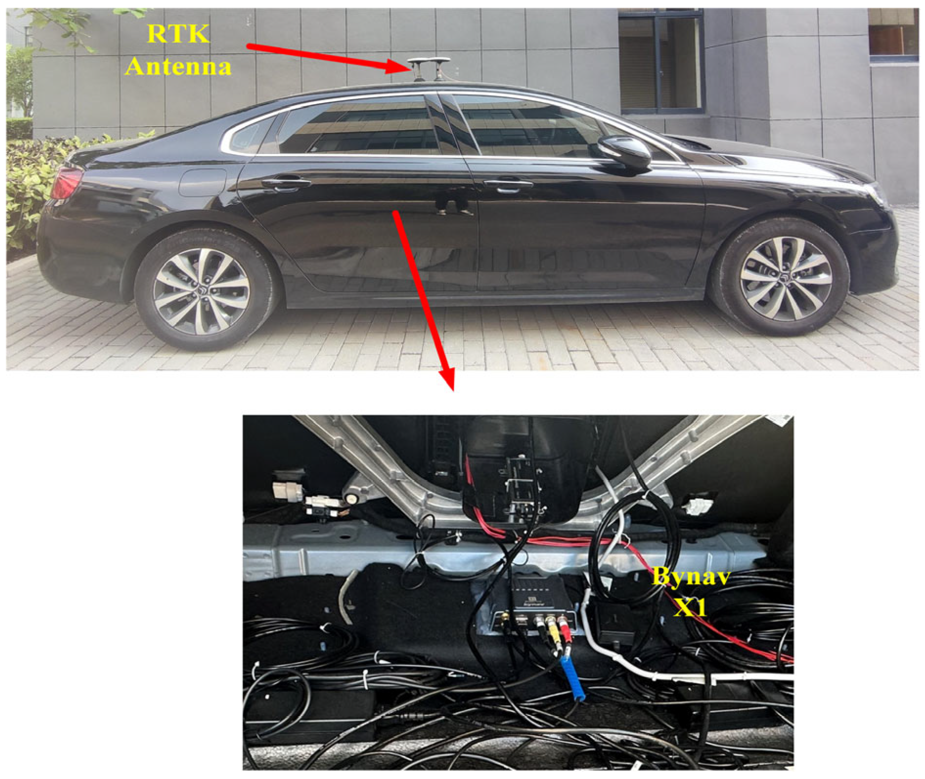
To evaluate the performance of the proposed method, we built the testbed for the IMU/GNSS/ODO integrated navigation system. The data acquisition vehicle is shown in Figure 4. The sensors used are all commercial and the specific parameters are shown in

Table 2. Parameters of relevant navigation sensors.

Sensors	Parameter	Value
IMU	Gyro Bias instability	0.9°/h
	Accelerometer Bias instability	0.01 mg
	Accelerometer RMS noise	0.5 mg
	Gyro RMS noise	0.007°/s
GNSS RTK	Positional accuracy	1.5 cm + 1 ppm
Odometer	Positional accuracy	1% × Distance

. The sampling frequency of the MEMS-IMU SCHA634-D03 is set at 100 Hz and the frequency of the Bynav X1 GNSS receiver is at 5 Hz. We use RTK mode to obtain the positioning results in the experiments. The ODO is mounted on the rear wheel bearing. In addition, forward and backward filtering postprocessing is used to provide the ground truth. We run the algorithms on a desktop computer equipped with an Intel i7-12700 at 2.10 GHz and 32 GB RAM and the size of the sliding window is set to 1 s.

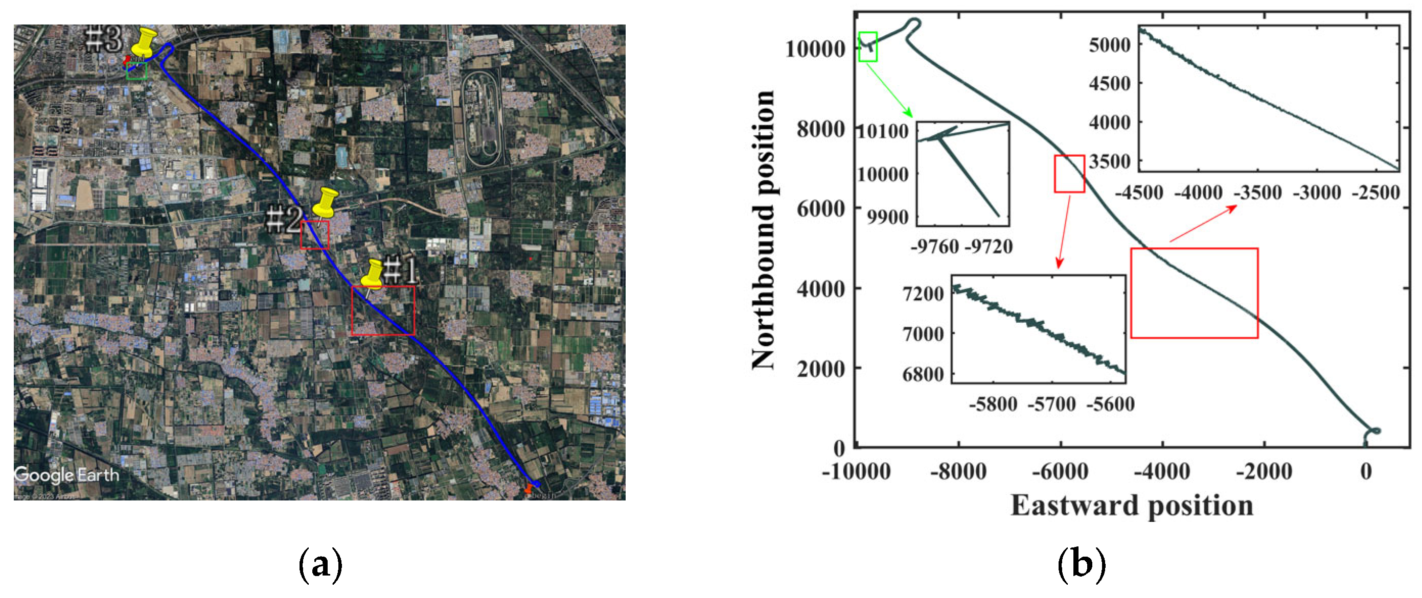
The vehicle-mounted test was conducted on a viaduct in the Daxing district, Beijing, with an average speed of 16 km/h and a duration of 1190 s. The specific trajectory is shown in Figure 5a. The experimental environment includes up and down the viaduct and stable driving. However, in complex urban environments, GNSS signals are highly susceptible to interference; thus, the SD output from the GNSS board is not completely reliable. We choose #1 and #2, which have no faults in raw data then add faults manually to simulate the situation where there are faults in the GNSS signals but the SD judgment is completely ineffective. To verify the effectiveness and robustness of the proposed algorithm, three sections of the trajectory including two typical fault types are selected for verification:

(1)

#1 and #2 are selected during the stable driving process in an open environment, which means that the original data in these segments are error-free. The complete failure of SD detection, which is the worst-case scenario, can be simulated by adding errors. To simulate the ramp and step fault of the satellite, we add slow-growth faults at 400 s to 580 s (#1), lasting 180 s, and step faults at 700 s to 730 s (#2), lasting 30 s, to the latitude and longitude of the satellite. The GNSS anomaly detection algorithm is validated using all segments including simulation errors.

(2)

#1 and #3 are selected to verify the effectiveness of SAWE-FGO. #3 (from 1153 s to 1162 s) is a winding road where the vehicle passes through the staggered elevation before the turn, with continuous random jump points in the raw data (from 1138 s to 1152 s).

The GNSS output trajectory after adding the faults is shown in Figure 5b, with the distance information relative to the start point (0 s).

4.1. Validation of the GNSS Anomaly Detection Algorithm

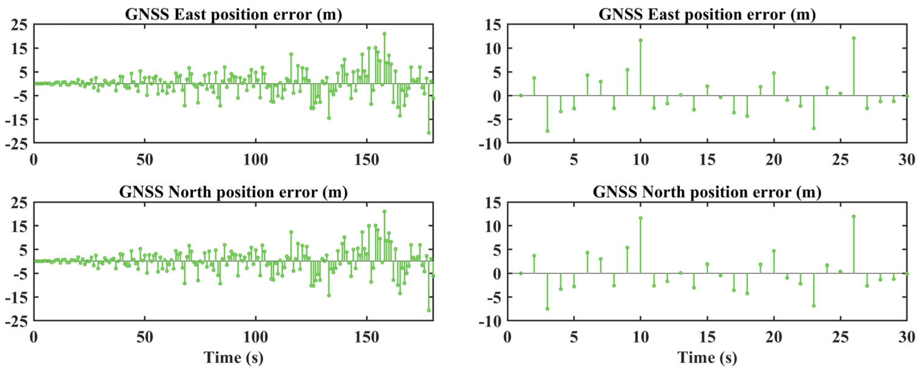
In the simulation, the whole duration is about 180 s in #1 and 30 s in #2; the GNSS measurements are available during these two periods of time. Slow-growth faults and step faults are added to the latitude and longitude, respectively. The size of the added faults in #1 (group A) and #2 (group B) is shown in Figure 6.

We apply the proposed GNSS anomaly detection method to the entire trajectory segment, which includes both real and simulated faults, for comprehensive evaluation. To illustrate the specific results of typical failure types, we select two representative segments of the trajectory (#1 and #2).

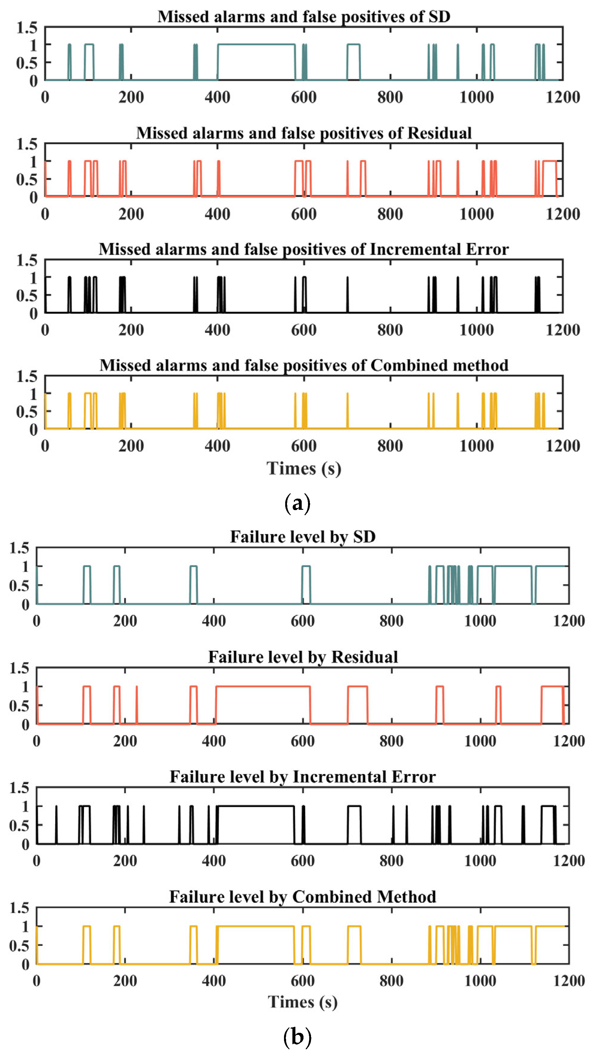
The missed alarms and false positives of different methods are demonstrated in Figure 7a. For the judgment curves, a value of 1 means missed alarms or false positives and a value of 0 means normal detection. Meanwhile, the failure level by different methods is shown in Figure 7b. For the judgment curves, a value of 1 signifies that the detection method detects a perceived fault and a value of 0 denotes no fault.

As Figure 7a illustrates, the SD statistics have a long duration during 400 s to 580 s, while the residual statistics identify the missed detection. However, a 17 s duration is required for the residual statistics parameter to fall under the fault alarm shoulder. Meanwhile, a new fault appears in the raw data at 597 s. As shown in Figure 7b, the residual detection is unable to distinguish between the two adjacent faults and it is straightforward to determine that all of them are abnormal from 404 s to 618 s. The proposed method is composed of an SD test unit, a residual test unit, and an incremental error unit, which significantly reduces missed alarms. As

Table 3. Statistical results of missed alarms and false positives.

Error Level	SD Criterion	Residuals Criterion	Incremental Error Criterion	Combined Method
Number of false detections	276	151	69	74
Number of missed alarms	272	38	48	50
Number of false positives	4	113	21	24
Missed alarm rate	0.93	0.13	0.16	0.17
False alarm rate	0.009	0.14	0.02	0.02

shows, the missed alarm rate of the combined method is reduced by 81.7% compared with the SD criterion and the false alarm rate of the combined method is reduced by 85.7% compared with the residual criterion.

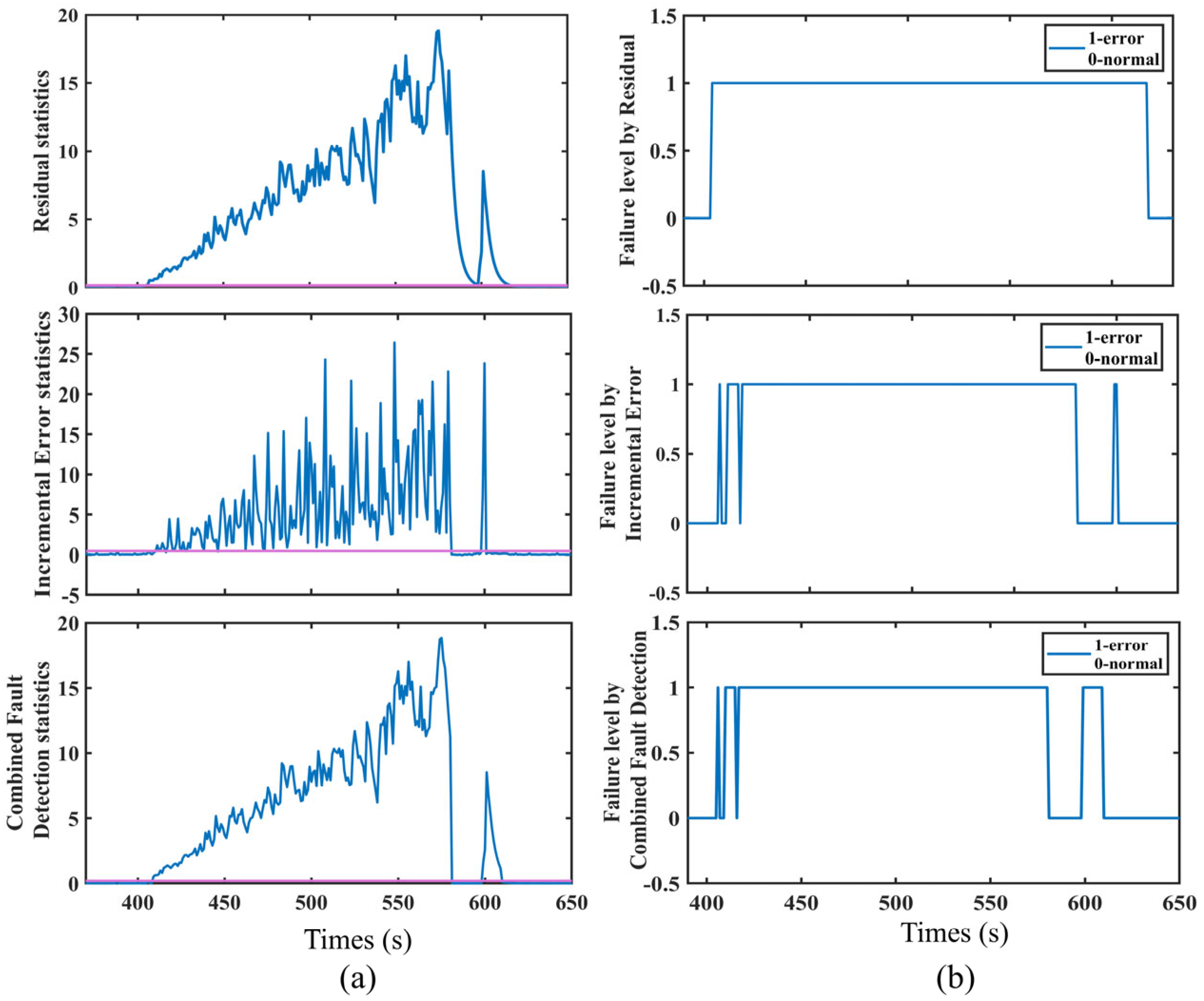
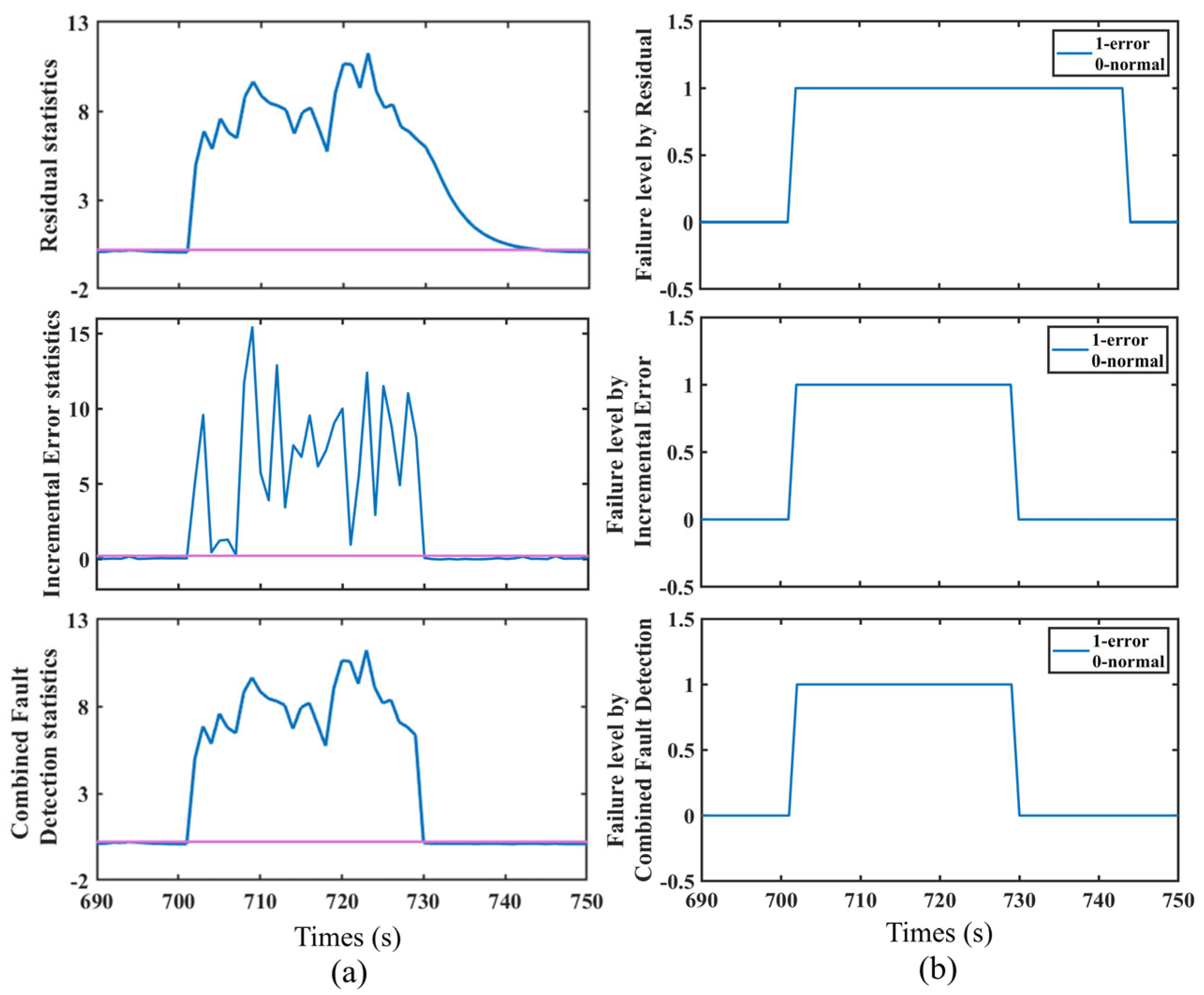
In addition, to represent the performance of the use of the incremental error criterion to assist the residual criterion in the case of complete failure of SD detection, #1 and #2 are selected to evaluate the advantages of the proposed method by comparing the detection and recovery ability for different types of faults, as shown in Figure 8 and Figure 9. Figure 8 shows the results for group A in ramp failure, while Figure 9 presents the results for group B in step failure. The statistical curves of residual, incremental error, and combined fault detection methods are compared in Figure 8a and Figure 9a where the pink line represents the threshold. Meanwhile, the judgment results of these methods are presented in Figure 8b and Figure 9b. For the judgment curves, a value of 1 means that the detection method detects a perceived fault and a value of 0 means normal. The fault detection delays for different detection methods are listed in

Table 4. Delayed time of fault detection and recovery.

Failure Type	Group	Residuals Criterion	Incremental Error Criterion	Combined Method
Slope Failure	A detection	4 s	9 s	4 s
	A recovery	38 s	1 s	1 s
Step Failure	B detection	1 s	2 s	1 s
	B recovery	13 s	0 s	0 s

.

Among the results presented in Table 4, the following conclusions can be easily found:

(1) For step faults, all methods are able to detect the start of the fault quickly. For ramp failure, the combined fault detection method chooses the minimum detection time due to the sensitivity of the residual method.

(2) The proposed method can recover after the failure termination, with a 92–97% reduction in delay compared to the residual method.

(3) In group A, it is not hard to see original faults appearing after the end of adding faults. In Figure 8, the residual method cannot distinguish between different faults, which is not possible for multiple-failure detection. Instead, the proposed method overcomes the drawback of the residual method in failure recovery, which can detect second faults.

Fault delay detection and recovery usually adversely affect the parameter estimation, making the AWE not optimal. Therefore, the proposed detection algorithm is used to solve this problem in the next part, which can quickly and accurately determine the moment when the system returns to normal and then switch to the normal weighting mode.

4.2. Comparison of Performance between Different Information Fusion Methods

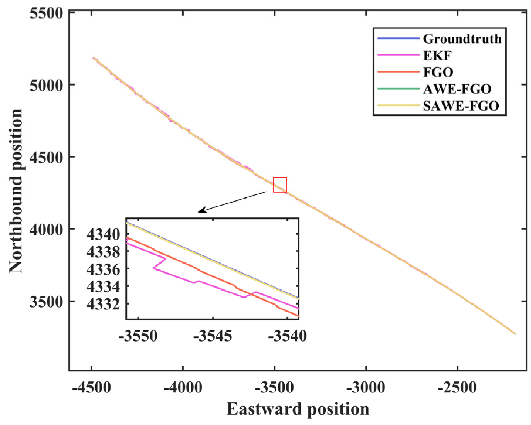
To verify the effectiveness of the switching adaptive weighting estimation (SAWE), #1 is selected for verification. We compared our methods with the EKF method, which is commonly used in engineering applications, and the traditional FGO method. The elapsed time of all data for the FGO algorithm with the equipped CPU is about 18 s. Figure 10, Figure 11 and Figure 12 demonstrate the localization results produced by each algorithm.

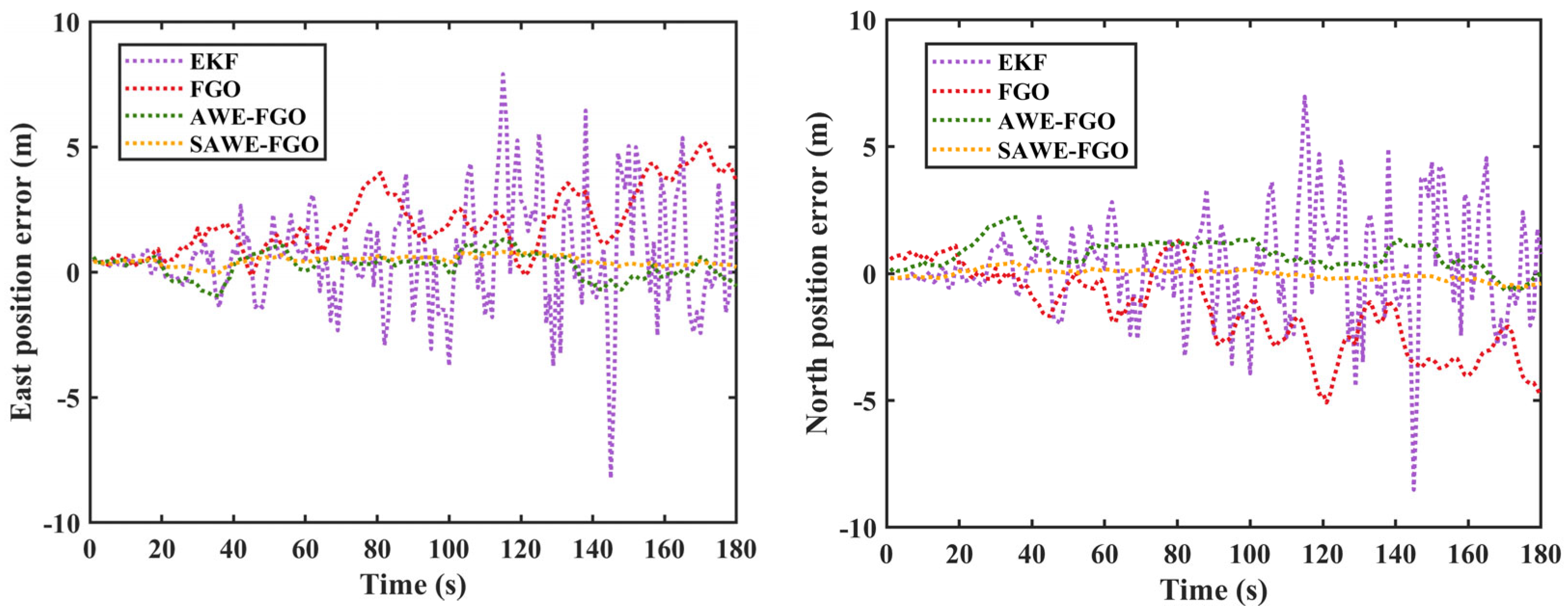
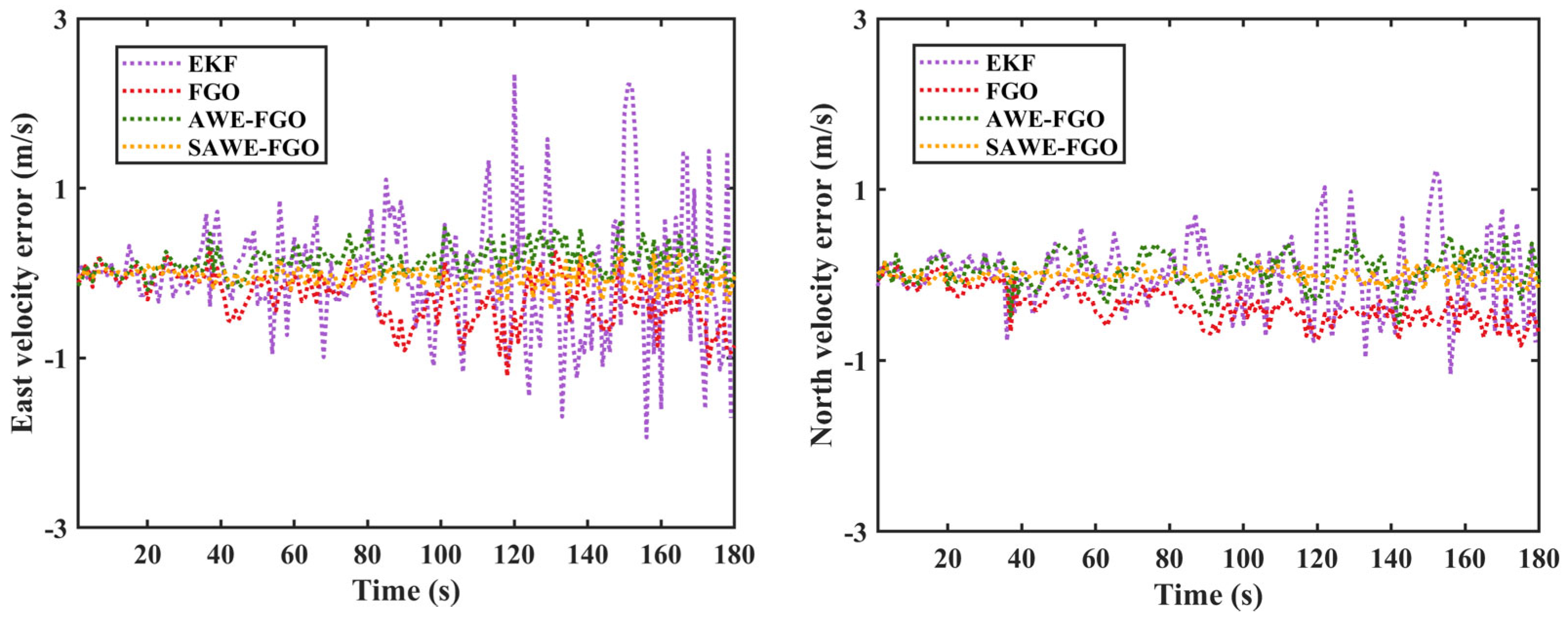
The traces of the different algorithms are shown in Figure 10. It can be seen that, after the addition of the damp faults, there are obvious fluctuations in EKF. The smoothing effect of FGO is better than that of the EKF; however, there are still some large errors here. Instead, there is not a significant decrease in the navigation accuracy of the AWE-FGO and SAWE-FGO. Figure 11 and Figure 12 show the position errors and velocity errors, respectively. We can see that the position and velocity errors are remarkably reduced using AWE-FGO and SAWE-FGO. The position results are shown in

Table 5. STD and RMSE of position and velocity errors for different algorithms in #1.

Error	Method	STD	RMSE
East position error (m)	EKF	2.155	2.248
	FGO	1.304	2.396
	AWE-FGO	0.509	0.570
	SAWE-FGO	0.189	0.489
North position error (m)	EKF	2.051	2.062
	FGO	1.642	2.227
	AWE-FGO	0.586	0.954
	SAWE-FGO	0.206	0.208
East velocity error (m/s)	EKF	0.721	0.720
	FGO	0.297	0.410
	AFGO	0.174	0.206
	SAWE-FGO	0.122	0.132
North velocity error (m/s)	EKF	0.393	0.392
	FGO	0.210	0.409
	AFGO	0.168	0.206
	SAWE-FGO	0.131	0.078

.

For the eastward position, the STD values of FGO and AWE-FGO reach 1.304 m and 0.509 m, respectively, while EKF reaches 2.155 m. The STD of FGO improved by 39.4% compared to EKF. Similarly, for the northward position, the STD improves by 19.9%. It can be seen that the positioning accuracy of EKF and FGO is comparable. After applying AWE to the FGO, the errors reduce noticeably in Table 5, which shows the effectiveness of the proposed AWE method. Moreover, with the help of SAWE via SAWE-FGO, the position errors decrease to 0.489 m and 0.208 m, respectively, resulting in a further improvement in accuracy from AWE-FGO. RMSE can reflect the deviation of the estimated value from the reference value. The use of RMSE can assess the impact of outliers on navigation and reflect the navigation accuracy and robustness. It can be seen that the RMSE of AWE-FGO is significantly smaller than that of EKF and FGO, with reductions of 76.3% and 57.2% in eastward and northward positions, respectively. When the traditional factor graph algorithm is enhanced by SAWE-FGO, the position accuracy improves by 80%. The higher accuracy and robustness of the proposed method depend on the fact that the SAWE-FGO can recognize the end time of faults and adjust the corresponding covariance according to the error changes, which makes the weighting more accurate. In contrast, the traditional factor graph model does not take into account the exceptions of sensor measurements in the information fusion process, which leads to a decrease in navigation accuracy.

In addition, we interestingly discovered that the fault detection delay has a much greater effect on the turnaround than the straight line. Therefore, we choose #3 for additional validation. It can be seen in Figure 5b that there are random jump points in the GNSS signals before passing a turnaround section (#3) as the road crosses the viaduct for a while. As shown in Figure 13, we use the SAWE-FGO method compared with full use of the AWE-FGO method for the selected trajectory (#3). It can be seen that the AWE-FGO method causes an error of about 1 m in the northward position, while the SAWE-FGO method has a maximum of only 0.1 m, which validates the effectiveness of SAWE.

4.3. Experimental Validation Using an Open-Source Dataset

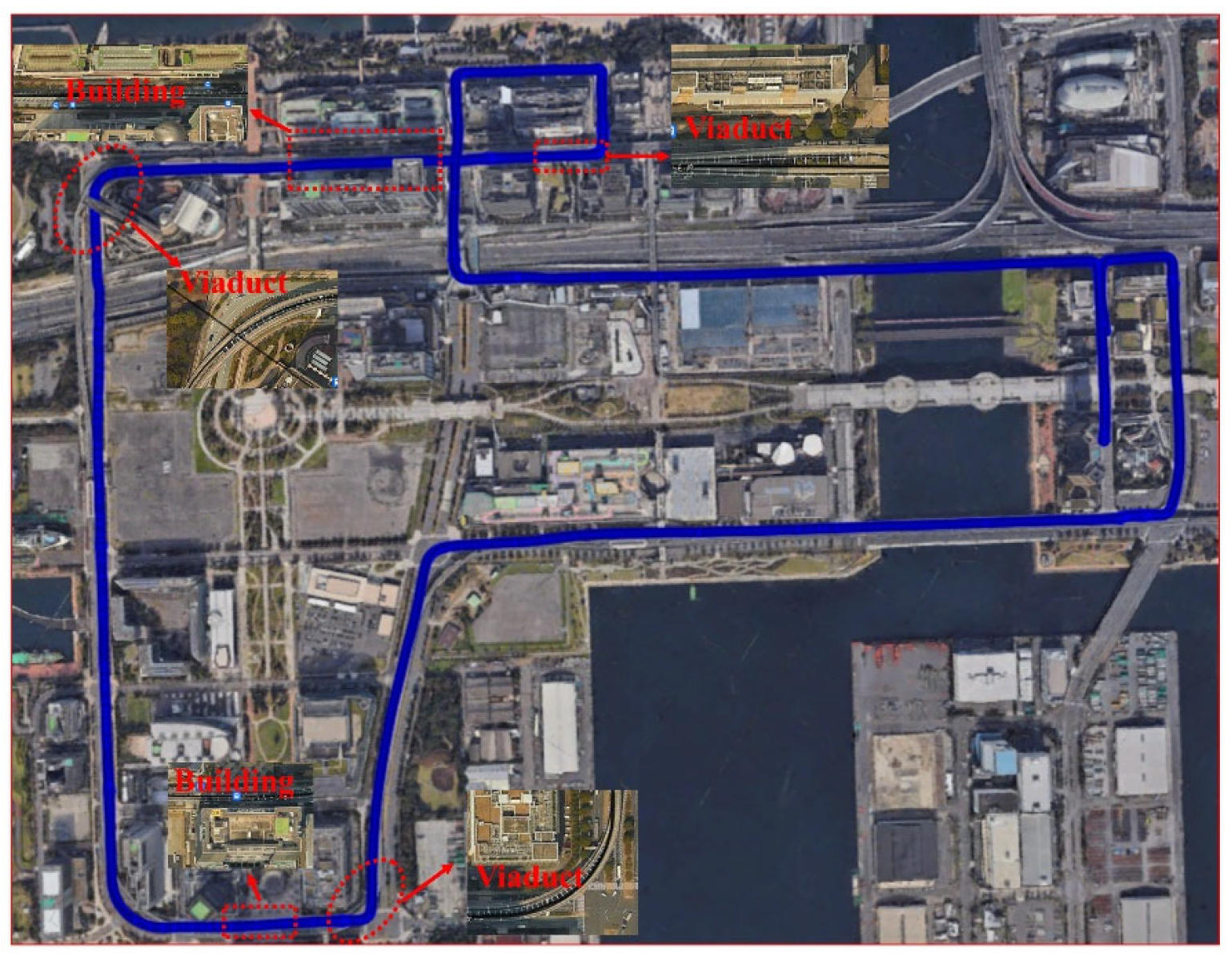
To challenge the performance of the proposed fault detection algorithm and adaptive weight estimation strategy, we test the proposed algorithms on the open-source dataset collected in the Odaiba districts of Tokyo Urban Canyons [45], which has denser buildings and multiple viaducts compared with the experimental environment in which we collected data. In other words, the selected open-source dataset is collected in a typical urban canyon environment with a higher percentage of multipath/NLOS effects.

Figure 14 shows the vehicle traveling trajectory provided by the high-precision INS/RTK positioning results. It can be seen that the road condition is quite complicated, which not only contains straight lines and turning sections but also passes through dense buildings and several viaducts.

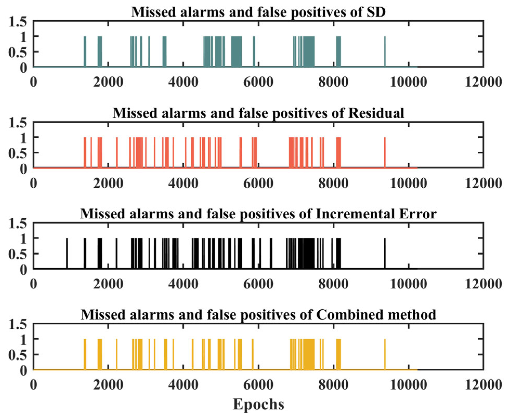
In order to validate the effectiveness of the proposed algorithm, we performed fault detection validation and adaptive weight estimation validation on this dataset, respectively. The missed alarms and false positives of different methods are demonstrated in Figure 15. For the judgment curves, a value of 1 means missed alarms and false positives and a value of 0 means normal detection.

Figure 15 shows that, in typical urban canyon environments, GNSS signals are significantly disturbed by multipath/NLOS effects, resulting in frequent anomalies in the SD values of GNSS outputs.

As

Table 6. Statistical results of missed alarms and false positives.

Error Level	SD Criterion	Residuals Criterion	Incremental Error Criterion	Combined Method
Number of false detections	1220	1100	1470	980
Number of missed alarms	1210	430	900	720
Number of false positives	10	670	570	260
Missed alarm rate	0.63	0.22	0.46	0.37
False alarm rate	0.001	0.08	0.07	0.03

shows, the missed alarm rate of the combined method is reduced by 41% compared with the SD criterion and the false alarm rate of the combined method is reduced by 62% compared to the residual criterion.

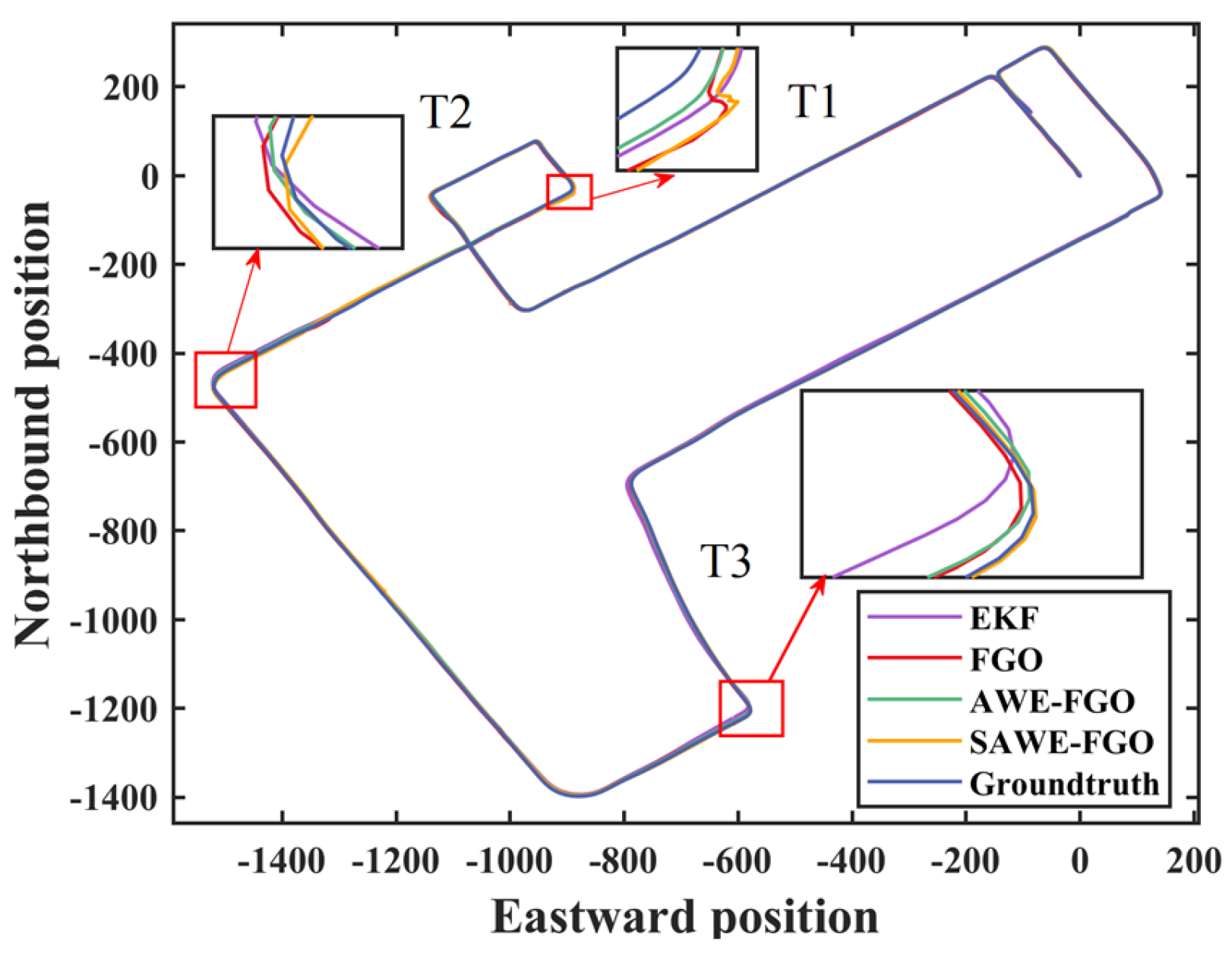
A comparison of performance between different information fusion methods is shown in Figure 16 and Figure 17.

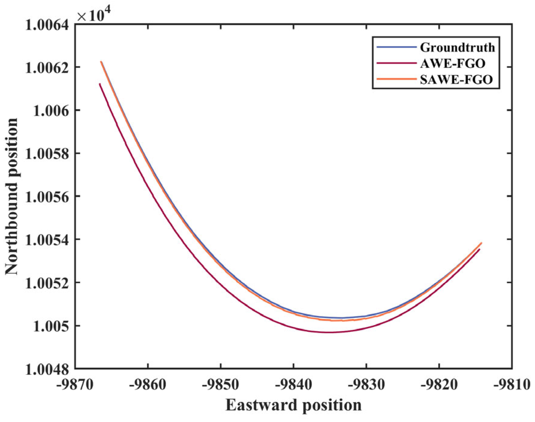
The traces of the different algorithms are shown in Figure 16. The three zoomed-in trajectories (T1, T2, and T3) correspond to three elevated segments. With the AWE method, the trajectories at the corners are significantly smoother and the corresponding errors are smaller than those of EKF and FGO. When the system is operating in switchable modes, there is a further reduction in error at corners, except for section T1, which occurs because the fault detection algorithm fails to detect partial faults in the segment, failing to switch up to AWE mode.

Figure 17 shows the position error. It can be seen that the EKF has a large error and FGO has a relatively reduced error, while the AWE-FGO significantly reduces the error. The position results are shown in

Table 7. STD and RMSE of position errors for different algorithms.

Error	Method	STD	RMSE
East position error (m)	EKF	3.656	4.115
	FGO	1.438	2.057
	AWE-FGO	1.108	1.282
	SAWE-FGO	0.906	1.805
North position error (m)	EKF	2.320	2.354
	FGO	1.858	2.631
	AWE-FGO	1.273	1.605
	SAWE-FGO	1.088	1.509

.

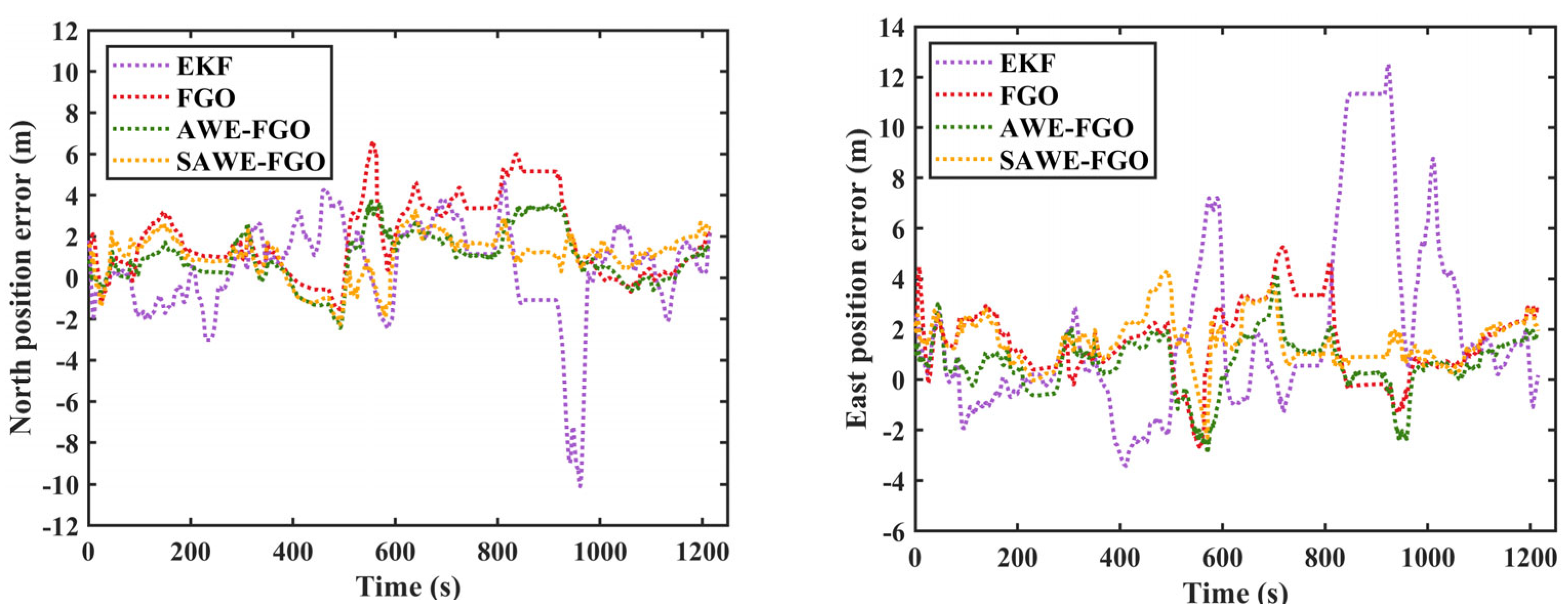
For the eastward position, the STD values of AWE-FGO and SAWE-FGO reach 1.108 m and 0.906 m, respectively. The position accuracy of AWE-FGO improved by 37.7% compared with FGO. Relative to EKF, the AWE-FGO errors are reduced by 68.8%. Similarly, for the northward position, the position accuracy of AWE-FGO improves by 39.0% compared with FGO. Compared to EKF, the AWE-FGO errors are reduced by 45.1%. While SAWE-FGO significantly reduces errors in the northward position, it does not perform as well in the eastward position due to the failure of fault detection at T1.

In short, the errors are reduced significantly with the help of AWE. Moreover, the proposed fault detection method based on multi-conditional analysis is also validated on the challenging dataset. With the aid of fault detection, the SAWE exhibits less positional error. Since the selection of the threshold values directly affects the effectiveness of fault detection, we need to continue to improve and explore the criteria for threshold selection in the future.

5. Conclusions

To improve the accuracy and robustness of the integrated navigation system in complex urban environments, this paper proposes a robust factor graph optimization method with switchable adaptive weight estimation. Aiming at the shortcomings of the existing factor graph algorithms, an adaptive covariance estimation factor graph navigation algorithm is proposed, which effectively suppresses the impact of GNSS faults on the accuracy of the navigation system. In addition, we also propose a GNSS anomaly detection strategy based on multi-conditional analysis, which improves the system fault detection capability and effectively improves the robustness of the system. The superiority and robustness of the proposed method relative to other methods have been verified in vehicle experiments. The positioning accuracy of the proposed AWE-FGO method is improved by more than 60% compared to the traditional FGO algorithm. Moreover, the proposed fault detection method is effective in detecting the end of the fault and greatly reduces the effect of delay on parameter estimation. Therefore, SAWE-FGO can be used to produce superior navigational results. Furthermore, we verified the performance of the algorithm on a real urban canyon dataset and the results show that the proposed method improves the navigation accuracy by more than 30% compared to the FGO algorithm. In more complex environments, the threshold selection of faults is more difficult and the improvement of threshold selection criteria will be one of the focuses of future work.

References

- Groves, P. Principles of GNSS, Inertial, and Multisensor Integrated Navigation Systems; Artech: Morristown, NJ, USA, 2007. [Google Scholar]
- Inside GNSS. Multipath vs. NLOS Signals; Inside GNSS—Global Navigation Satellite Systems Engineering, Policy, and Design: Red Bank, NJ, USA, 2013. [Google Scholar]
- Boguspayev, N.; Akhmedov, D.; Raskaliyev, A.; Kim, A.; Sukhenko, A. A Comprehensive Review of GNSS/INS Integration Techniques for Land and Air Vehicle Applications. Appl. Sci. 2023, 13, 4819. [Google Scholar] [CrossRef]
- Mu, M.; Zhao, L. A GNSS/INS-Integrated System for an Arbitrarily Mounted Land Vehicle Navigation Device. GPS Solut. 2019, 23, 112. [Google Scholar] [CrossRef]
- Lou, T.-S.; Chen, N.-H.; Chen, Z.-W.; Wang, X.-L. Robust Partially Strong Tracking Extended Consider Kalman Filtering for INS/GNSS Integrated Navigation. IEEE Access 2019, 7, 151230–151238. [Google Scholar] [CrossRef]
- Allotta, B.; Caiti, A.; Costanzi, R.; Fanelli, F.; Fenucci, D.; Meli, E.; Ridolfi, A. A New AUV Navigation System Exploiting Unscented Kalman Filter. Ocean Eng. 2016, 113, 121–132. [Google Scholar] [CrossRef]
- Arasaratnam, I.; Haykin, S. Cubature Kalman Filters. IEEE Trans. Autom. Control 2009, 54, 1254–1269. [Google Scholar] [CrossRef]
- Bell, B.M.; Cathey, F.W. The Iterated Kalman Filter Update as a Gauss-Newton Method. IEEE Trans. Autom. Control 1993, 38, 294–297. [Google Scholar] [CrossRef]
- Indelman, V.; Williams, S.; Kaess, M.; Dellaert, F. Information Fusion in Navigation Systems via Factor Graph Based Incremental Smoothing. Robot. Auton. Syst. 2013, 61, 721–738. [Google Scholar] [CrossRef]
- Wen, W.; Bai, X.; Kan, Y.C.; Hsu, L.-T. Tightly Coupled GNSS/INS Integration via Factor Graph and Aided by Fish-Eye Camera. IEEE Trans. Veh. Technol. 2019, 68, 10651–10662. [Google Scholar] [CrossRef]
- Wen, W.; Pfeifer, T.; Bai, X.; Hsu, L.-T. It Is Time for Factor Graph Optimization for GNSS/INS Integration: Comparison between FGO and EKF. arXiv 2020, arXiv:2004.10572. [Google Scholar]
- Zeng, Q.; Chen, W.; Liu, J.; Wang, H. An Improved Multi-Sensor Fusion Navigation Algorithm Based on the Factor Graph. Sensors 2017, 17, 641. [Google Scholar] [CrossRef] [PubMed]
- Dai, J.; Liu, S.; Hao, X.; Ren, Z.; Yang, X. UAV Localization Algorithm Based on Factor Graph Optimization in Complex Scenes. Sensors 2022, 22, 5862. [Google Scholar] [CrossRef] [PubMed]
- Xu, J.; Yang, G.; Sun, Y.; Picek, S. A Multi-Sensor Information Fusion Method Based on Factor Graph for Integrated Navigation System. IEEE Access 2021, 9, 12044–12054. [Google Scholar] [CrossRef]
- Dehghannasiri, R.; Esfahani, M.S.; Dougherty, E.R. Intrinsically Bayesian Robust Kalman Filter: An Innovation Process Approach. IEEE Trans. Signal Process. 2017, 65, 2531–2546. [Google Scholar] [CrossRef]
- Zhao, D.; Hancock, C.M.; Roberts, G.W.; Jin, S. Cycle Slip Detection during High Ionospheric Activities Based on Combined Triple-Frequency GNSS Signals. Remote Sens. 2019, 11, 250. [Google Scholar] [CrossRef]
- Yuan, H.; Zhang, Z.; He, X.; Xu, T.; Xu, X.; Zang, N. Real-Time Cycle Slip Detection and Repair Method for BDS-3 Five-Frequency Data. IEEE Access 2021, 9, 51189–51201. [Google Scholar] [CrossRef]
- Sun, K.; Zeng, Q.; Liu, J.; Wang, S. Fault Detection of Resilient Navigation System Based on GNSS Pseudo-Range Measurement. Appl. Sci. 2022, 12, 5313. [Google Scholar] [CrossRef]
- Roysdon, P.F.; Farrell, J.A. GPS-INS Outlier Detection & Elimination Using a Sliding Window Filter. In Proceedings of the 2017 American Control Conference (ACC), Seattle, WA, USA, 24–26 May 2017; pp. 1244–1249. [Google Scholar]
- Wen, W.; Meng, Q.; Hsu, L.-T. Integrity Monitoring for GNSS Positioning via Factor Graph Optimization in Urban Canyons. In Proceedings of the 34th International Technical Meeting of the Satellite Division of The Institute of Navigation (ION GNSS+ 2021), St. Louis, MO, USA, 20–24 September 2021; pp. 1508–1515. [Google Scholar]
- Hu, Y.; Li, H.; Liu, W. Robust Factor Graph Optimisation Method for Shipborne GNSS/INS Integrated Navigation System. IET Radar Sonar Navig. 2023, 17, 1–17. [Google Scholar] [CrossRef]
- Zhang, C.; Zhao, X.; Pang, C.; Li, T.; Zhang, L. Adaptive Fault Isolation and System Reconfiguration Method for GNSS/INS Integration. IEEE Access 2020, 8, 17121–17133. [Google Scholar] [CrossRef]
- Su, S.; Dai, H.; Cheng, S.; Lin, P.; Hu, C.; Lv, B. A Robust Magnetic Tracking Approach Based on Graph Optimization. IEEE Trans. Instrum. Meas. 2020, 69, 7933–7940. [Google Scholar] [CrossRef]
- Sünderhauf, N.; Protzel, P. Switchable Constraints for Robust Pose Graph SLAM. In Proceedings of the 2012 IEEE/RSJ International Conference on Intelligent Robots and Systems, Vilamoura-Algarve, Portugal, 7–12 October 2012; pp. 1879–1884. [Google Scholar]
- Pfeifer, T.; Lange, S.; Protzel, P. Dynamic Covariance Estimation—A Parameter Free Approach to Robust Sensor Fusion. In Proceedings of the 2017 IEEE International Conference on Multisensor Fusion and Integration for Intelligent Systems (MFI), Daegu, Republic of Korea, 16–18 November 2017; pp. 359–365. [Google Scholar]
- Wei, X.; Li, J.; Zhang, D.; Feng, K. An Improved Integrated Navigation Method with Enhanced Robustness Based on Factor Graph. Mech. Syst. Signal Process. 2021, 155, 107565. [Google Scholar] [CrossRef]
- Lesouple, J.; Robert, T.; Sahmoudi, M.; Tourneret, J.-Y.; Vigneau, W. Multipath Mitigation for GNSS Positioning in an Urban Environment Using Sparse Estimation. IEEE Trans. Intell. Transp. Syst. 2019, 20, 1316–1328. [Google Scholar] [CrossRef]
- Yi, B.; Lee, M.A.; Kloss, A.; Martín-Martín, R.; Bohg, J. Differentiable Factor Graph Optimization for Learning Smoothers. In Proceedings of the IEEE/RSJ International Conference on Intelligent Robots and Systems (IROS), Prague, Czech Republic, 27 September–1 October 2021. [Google Scholar]
- Nam, D.V.; Gon-Woo, K. Learning Type-2 Fuzzy Logic for Factor Graph Based-Robust Pose Estimation with Multi-Sensor Fusion. IEEE Trans. Intell. Transp. Syst. 2023, 24, 3809–3821. [Google Scholar] [CrossRef]
- Chang, L.; Niu, X.; Liu, T. GNSS/IMU/ODO/LiDAR-SLAM Integrated Navigation System Using IMU/ODO Pre-Integration. Sensors 2020, 20, 4702. [Google Scholar] [CrossRef]
- Bai, S.; Lai, J.; Lyu, P.; Cen, Y.; Ji, B. Improved Preintegration Method for GNSS/IMU/In-Vehicle Sensors Navigation Using Graph Optimization. IEEE Trans. Veh. Technol. 2021, 70, 11446–11457. [Google Scholar] [CrossRef]
- Kschischang, F.R.; Frey, B.J.; Loeliger, H.-A. Factor Graphs and the Sum-Product Algorithm. IEEE Trans. Inf. Theory 2001, 47, 498–519. [Google Scholar] [CrossRef]
- Barfoot, T.D. State Estimation for Robotics; Cambridge University Press: Cambridge, UK, 2017; ISBN 1-108-50971-1. [Google Scholar]
- Dellaert, F.; Kaess, M. Factor Graphs for Robot Perception. FNT Robot. 2017, 6, 1–139. [Google Scholar] [CrossRef]
- Carlone, L.; Kira, Z.; Beall, C.; Indelman, V.; Dellaert, F. Eliminating Conditionally Independent Sets in Factor Graphs: A Unifying Perspective Based on Smart Factors. In Proceedings of the 2014 IEEE International Conference on Robotics and Automation, ICRA 2014, Hong Kong, China, 31 May–7 June 2014; pp. 4290–4297. [Google Scholar]
- Kaess, M.; Ranganathan, A.; Dellaert, F. iSAM: Incremental Smoothing and Mapping. IEEE Trans. Robot. 2008, 24, 1365–1378. [Google Scholar] [CrossRef]
- Loeliger, H.-A.; Dauwels, J.; Hu, J.; Korl, S.; Ping, L.; Kschischang, F.R. The Factor Graph Approach to Model-Based Signal Processing. Proceedings of the IEEE 2007, 95, 1295–1322. [Google Scholar] [CrossRef]
- Moré, J.J. Levenberg–Marquardt Algorithm: Implementation and Theory; Springer: Berlin/Heidelberg, Germany, 1977. [Google Scholar]
- Kaess, M.; Johannsson, H.; Roberts, R.; Ila, V.; Leonard, J.; Dellaert, F. iSAM2: Incremental Smoothing and Mapping with Fluid Relinearization and Incremental Variable Reordering. In Proceedings of the 2011 IEEE International Conference on Robotics and Automation, Shanghai, China, 9–13 May 2011; pp. 3281–3288. [Google Scholar]
- Tardif, J.-P.; George, M.; Laverne, M.; Kelly, A.; Stentz, A. A New Approach to Vision-Aided Inertial Navigation. In Proceedings of the 2010 IEEE/RSJ International Conference on Intelligent Robots and Systems, Taipei, Taiwan, 18–22 October 2010; pp. 4161–4168. [Google Scholar]
- Chang, L.; Niu, X.; Liu, T.; Tang, J.; Qian, C. GNSS/INS/LiDAR-SLAM Integrated Navigation System Based on Graph Optimization. Remote Sens. 2019, 11, 1009. [Google Scholar] [CrossRef]
- Wu, Y.; Pan, X. Velocity/Position Integration Formula Part II: Application to Strapdown Inertial Navigation Computation. IEEE Trans. Aerosp. Electron. Syst. 2013, 49, 1024–1034. [Google Scholar] [CrossRef]
- Chiu, H.-P.; Williams, S.; Dellaert, F.; Samarasekera, S.; Kumar, R. Robust Vision-Aided Navigation Using Sliding-Window Factor Graphs. In Proceedings of the 2013 IEEE International Conference on Robotics and Automation, Karlsruhe, Germany, 6–10 May 2013; pp. 46–53. [Google Scholar]
- Carlone, L. State Estimation for Robotics [Bookshelf]. IEEE Control Syst. Mag. 2019, 39, 86–88. [Google Scholar] [CrossRef]
- Hsu, L.-T.; Kubo, N.; Wen, W.; Chen, W.; Liu, Z.; Suzuki, T.; Meguro, J. UrbanNav:An Open-Sourced Multisensory Dataset for Benchmarking Positioning Algorithms Designed for Urban Areas. In Proceedings of the 34th International Technical Meeting of the Satellite Division of the Institute of Navigation, ION GNSS+ 2021, St. Louis, MO, USA, 20–24 September 2021; pp. 226–256. [Google Scholar]
Figure 1.
Factor graph model of IMU/GNSS/ODO.
Figure 2.
Overview of the proposed IMU/GNSS/ODO integration via SAWE-FGO. The light blue area represents the factor graph optimization part. The green and orange area denotes the adaptive weighting estimation based on switching modes.
Figure 3.
Vector decomposition representation of GNSS and IMU-ODO preintegrated incremental error.
Figure 4.
Data collection scheme.
Figure 5.
The left figure (a) shows the trajectory in field tests. The right figure (b) shows the GNSS output trajectory.
Figure 6.
GNSS error in group A (left) and group B (right).
Figure 7.
(a) Missed alarms and false positives of different methods for the whole trajectory. (b) Fault detection of different methods for the whole trajectory.
Figure 8.
Fault detection results for ramp failure (group A). (a) The statistical curves of different methods. (b) The judgment results of different methods.
Figure 9.
Fault detection results for step failure (group B). (a) The statistical curves of different methods. (b) The judgment results of different methods.
Figure 10.
Positioning trace of different integrated navigation algorithms in #1.
Figure 11.
Position errors of different integrated navigation algorithms in #1.
Figure 12.
Velocity errors of different integrated navigation algorithms in #1.
Figure 13.
The comparison of trajectory in #3.
Figure 14.
The vehicle traveling trajectory.
Figure 15.
Missed alarms and false positives of different methods for the whole trajectory.
Figure 16.
Positioning trace of different integrated navigation algorithms.
Figure 17.
Position errors of different integrated navigation algorithms.